Multichannel Attention-Based TCN-GRU Network for Remaining Useful Life Prediction of Aero-Engines

Abstract

Predictive maintenance is a cornerstone of modern aerospace engineering, critical for maintaining the reliability and operational performance of aircraft engines. As a major component of prognostics and health management (PHM) technology, the accurate prediction of remaining useful life (RUL) enables proactive maintenance strategies, minimizes downtime, reduces costs, and enhances safety. This paper presents an innovative RUL prediction model designed specifically for aircraft engine applications. The model combines a temporal convolutional network (TCN) with multichannel attention and a gated recurrent unit (GRU) network. The framework begins with data pre-processing, followed by temporal feature extraction through an overlaying TCN network. Then, a multichannel attention mechanism fuses information from multiple TCN blocks, capturing rich feature representations. Finally, the fused data are processed by the GRU network to deliver precise RUL predictions. An improvement of at least 8.1% and 12.6% has been observed in two prediction metrics for the CMAPSS dataset when compared to other models.

1. Introduction

The aero-engine is the core component of an aircraft, and ensuring its safe running is critical to reducing the risk of aviation accidents. Aircraft engines are highly complex and sophisticated thermal machines [1,2,3]. The performance parameters of aero-engines degrade over the service life of an aircraft since most components of an aero-engine operate in a high-temperature, high-pressure environment. In particular, aero-engine components deteriorate slowly until they are no longer able to satisfy the operational requirements of the aircraft. In addition, unexpected failures can also accelerate the degradation of aero-engine components. Consequently, the remaining useful life (RUL) refers to the duration during which an aero-engine can safely perform its flight tasks [4,5].

Prognostics health management (PHM) technology is designed to assess the state of health of equipment and guide predictive repair and maintenance [6,7,8,9,10,11]. It includes fault forecasting and health management. For aircraft engines, precise RUL prediction facilitates the optimization of maintenance strategies, ensuring operational safety within defined thresholds and effectively reducing flight disruptions and emergency repairs [12,13]. In other words, health monitoring and prediction can avoid the high cost of engine failure or overhaul [14,15]. Obtaining data on the running status of equipment is an essential step in PHM. Sensors installed at various locations in the aero-engine record and store data. However, due to noise interference when the sensors collect data and the complexity of the engine itself, it is difficult to visually observe engine degradation from these data. Therefore, a worthwhile research problem is the modeling of the prediction of engine health from historical engine data.

Recently, the evolution of machine learning and deep learning algorithms has been a truly significant accomplishment in numerous domains, especially with these algorithms being applied in domains such as image, video, and text processing [16,17]. Deep learning methods are also employed in industry [18,19]. Predictive maintenance of aero-engines based on aero engine data is challenging. To enable predictive maintenance of aero-engines, researchers have leveraged sophisticated machine learning algorithms. In order to rely on historical data for predictive modeling, diverse methods have been implemented in an improved way. And these methods have been proven to show excellent results.

Currently, with the advancement of sensor technology and other related technologies, it is possible to obtain sufficient and complete information about the operation of the equipment. In the case of aircraft engines, the full cycle of data can be recorded, including the take-off, cruise, and landing processes. However, because of the complex structure and harsh operating conditions of aero-engines, the recorded data contain a lot of noise and non-linear characteristics. Neural network models show remarkable strengths in dealing with non-linear data. However, the analysis and pre-processing of data for specific cases, together with the design of the model, remain a challenge for researchers.

This paper presents a novel hybrid deep learning method for predicting the RUL of aero-engines. The major contributions of this are outlined as follows:

• A temporal convolutional network (TCN) is utilized. In the field of time series data modeling, TCN’s dilated convolution allows it to extract long-term dependencies into sequences.
• We designed an attention mechanism applied to multiple temporal resolutions and multiple features. For the output data from multiple TCN networks, an attention framework is designed to combine data from several time scales and channels. Consequently, multichannel attention fusion is formed, and the newly formed model is labeled MCA-TCN.
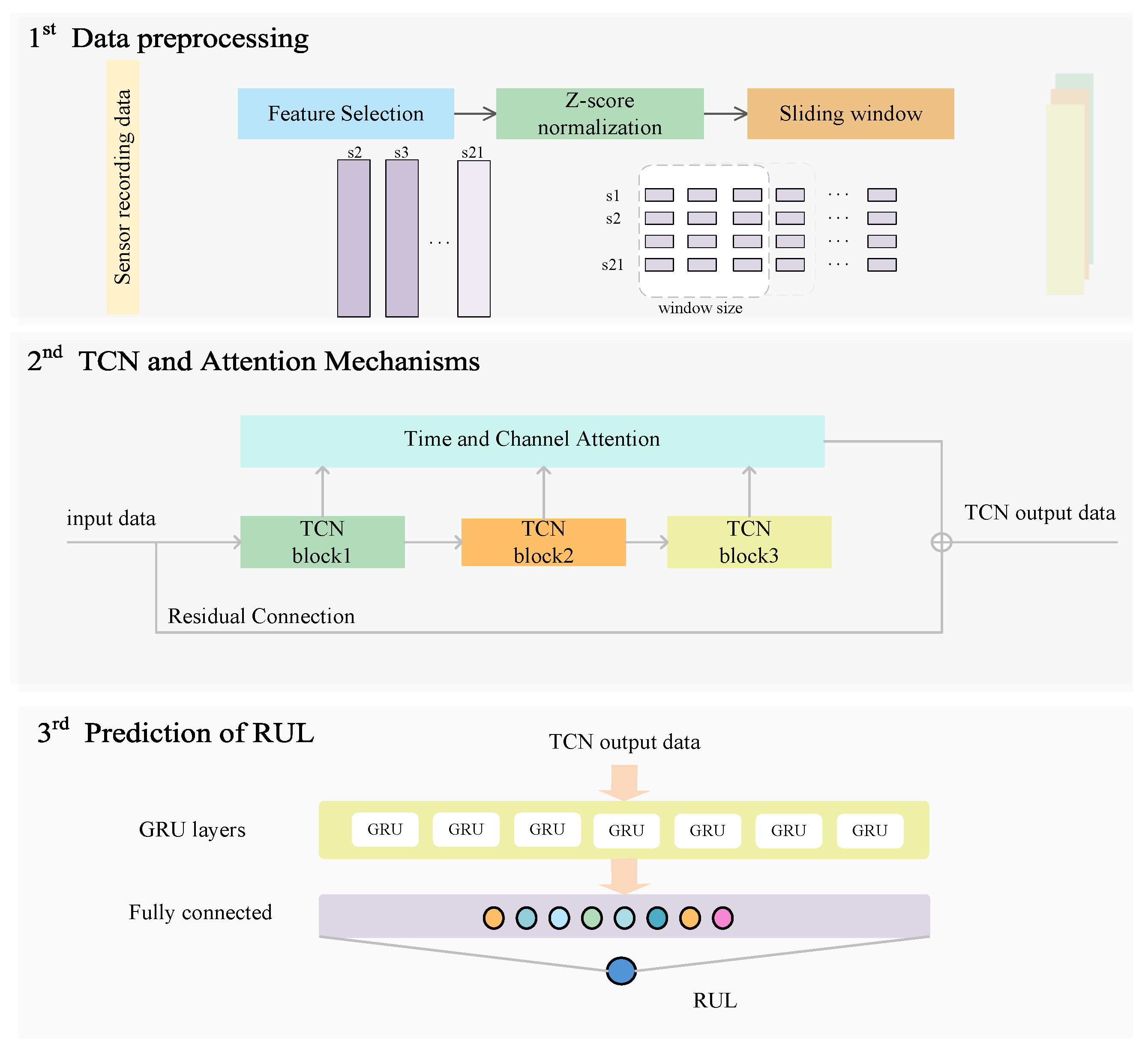
• The prediction of RUL is accomplished by gated cycle units. A layer of the GRU network is passed after all networks to further filter the effective information and achieve a high accuracy prediction.

The subsequent sections of this article are structured as follows: Section 2 discusses the related work. Section 3 provides a specific analysis of our proposed network. Section 4 introduces the datasets, explains the experiment, and provides the results along with their analysis. In Section 5, a conclusion is drawn for the article.

2. Related Work

To date, a wide variety of methods have been implemented by researchers to achieve reliable predictions of RUL [20,21,22,23]. Broadly, these strategies can be grouped into model-based, data-based, and hybrid approaches. Model-based approaches rely on specialized domain knowledge to describe data in terms of physical equations. However, with the advancement of computer arithmetic capabilities, it has become increasingly common to utilize efficient data-driven methods to derive the intrinsic connections of data from the data collected. The application of convolutional neural networks (CNNs) has led to exceptional outcomes in several fields like image recognition. Consequently, some studies have used CNN to attain the prediction of RUL. Ref. [20] introduced a data-driven approach for prognostic prediction based on deep convolutional neural networks (DCNN). It is also shown that DCNN outperforms other existing models. Li et al. [21] used multi-scale convolutional blocks to enhance the feature extraction capability within the original dataset. Furthermore, within the domain of RUL prediction, the Long-Short Term Memory (LSTM) model plays a prominent role in sequence modeling. A Dual-LSTM framework was proposed, which leverages LSTM for degradation analysis and RUL prediction [22]. The Dual-LSTM determines the health index for periods subsequent to the change point, which is subsequently employed to calculate the RUL. Ref. [24] employed the principal component analysis (PCA) technique in the data pre-processing session to extract the correlation between the data, which was then fed into the LSTM to forecast the RUL.

Recently, attention-based neural network architecture has driven AI across generations [25,26]. In the field of forecasting, it is necessary to further consider the role of attention [16]. Many researchers have combined attention mechanisms with classical neural networks to improve the accuracy of RUL predictions. Refs. [27,28] associated multiple attention mechanisms and temporal convolutional networks to demonstrate excellent performance, even on datasets with complex and challenging operating conditions and fault modes. It combines the feature variables with channel attention and temporal attention, which in turn feeds into a series of networks to predict the RUL. Li et al. [29] introduced a two-stage approach for battery capacity aging prediction. In the first step, the size of the time window is inferred by the false nearest neighbour (FNN) method. In the second step, a triple parallel attention network is utilized to extract features separately. And finally, a fully connected network is utilized for the purpose of RUL prediction.

A number of researchers have proposed effective networks for RUL prediction. However, most of these networks are stacked. The effectiveness of the attention mechanism has been well established, which allows us to pay attention to the correlations between the different levels, thus improving the forward propagation of effective information. Therefore, a method to combine the outputs of multiple TCN blocks is proposed. Moreover, this method achieves an increase in prediction accuracy.

3. Methodology

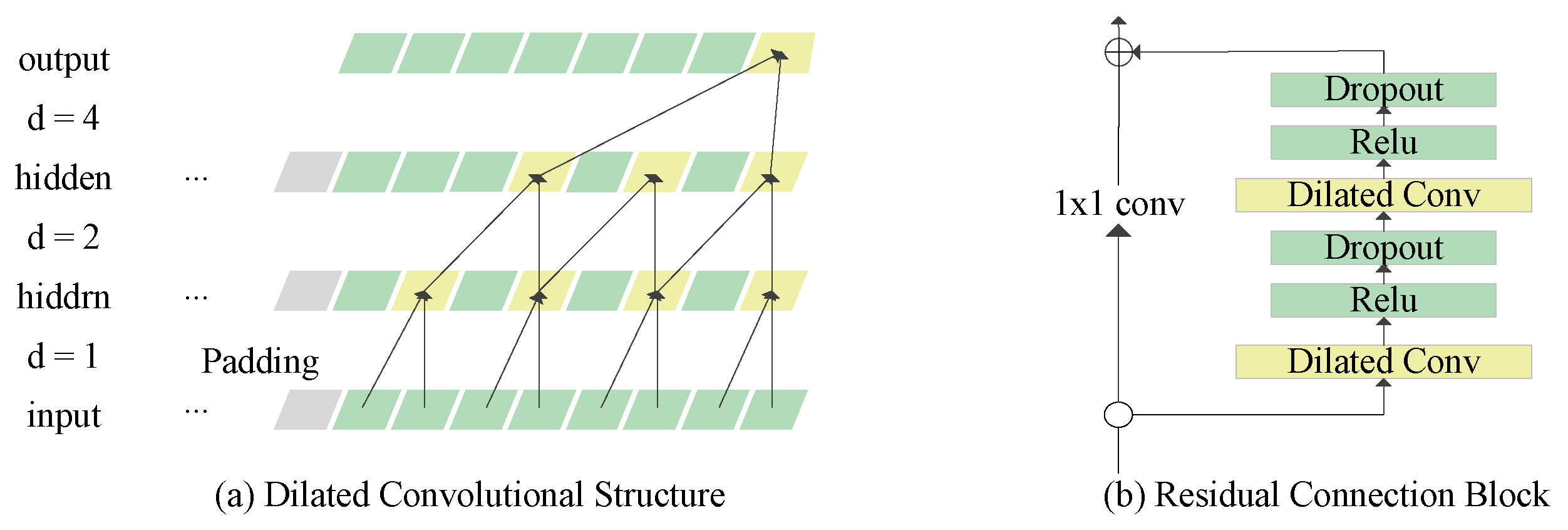
3.1. Temporal Convolutional Network

Temporal convolutional networks are the new network architecture based on CNNs [30]. It was originally proposed to resolve the sequence data model problem. Compared to recurrent neural networks, TCN demonstrates comparable performance in modeling sequential data due to its unique network sub-modules, with the most notable being the applications of dilated convolution and residual connections.

3.1.1. Dilated Convolutions

One-dimensional convolution is employed to extract features from one-dimensional sequential data, compared to the traditional two-dimensional convolution in image. However, common one-dimensional convolution improves the receptive field of the convolution kernel simply by increasing the size of the convolution kernel. For the purpose of acquiring dependencies over long periods of time in a sequence, it is necessary to superimpose multiple layers of convolutional networks. Dilated convolution solves this problem by setting the convolution kernel to skip part of the input to deal with the temporal modeling problem. The specific structure is shown in Figure 1. For a 1-D sequence input data $\mathbf{x}\in {\mathbb{R}}^n$ and the f in the convolution kernel, the dilated convolution is defined as:

$$F\left(s\right)=\left(\mathbf{x}{\ast }_{d}f\right)\left(s\right)=\sum _{i=0}^{k-1}f\left(i\right)·{\mathbf{x}}_{s-d·i}$$

(1)

where s is the element of the sequence, k is the kernel size, and d is the dilation size. The zero-padding techniques are often used to ensure that the length of the time series remains the same.

3.1.2. Residual Connections

In deep learning, increasing the depth of the neural network certainly improves the fit of the model. But it can also cause the problem of gradient vanish. The residual connection approach can alleviate this problem [31]. The residual block can be described as

$$y=f(\mathbf{x},W)+\mathbf{x}$$

(2)

where y is the output, $f(\mathbf{x},W)$ represents the output of the dilated convolution, and $\mathbf{x}$ is the input from the previous step of the network.

3.2. Multi-Temporal Feature Attention Mechanism

In the forward propagation of traditional neural network architectures, efficient information is fed into the next network step by step. Although TCN can obtain relevant information over long periods of time, the dilated convolutions at different scales are stacked up. Consequently, for better fusion of useful information from convolutional kernels of different time scales and extraction of fusion information across features, a method for integrating information across different time steps and channels is proposed, which can be regarded as an attention mechanism. The framework for attention calculation is based on the approach in [32]. The details are as in Figure 2.

(1)

For 1-D input data $X=(x_1,x_2,\dots ,x_T), x_t\in {\mathbb{R}}^d$, input the TCN block and obtain the output $X_{Block1}=(x_1,x_2,\dots ,x_T), x_t\in {\mathbb{R}}^d$;

(2)

After inputting n blocks, the connection data become $X_{con}=(x_1,x_2,\dots x_T,\dots x_{nT}), x_t\in {\mathbb{R}}^d$; then, after average pooling and 1-D convolution, the data become $X_{pooling}=(x_1,x_2,\dots x_T,\dots x_{nT}), x_t\in \mathbb{R}$;

(3)

Pooled information is transformed into less informative representations through the application of a fully-connected layer, and the dimensionality of the data is reduced through a second fully-connected layer;

(4)

Input sigmoid function to obtain the weight $weight=(w_1,w_2,\dots ,w_T,\dots w_{nT}),w_t\in R$, then multiply by elements, obtain weighted data $X_{weight}$, and the Softmax function is calculated as (3);

(5)

To reduce the amount of data, reshape the weighted data and sum in axis 1 to make the data and block output data the same size as one TCN block.

$$\mathrm{softmax}\left({\mathbf{X}}_{\mathbf{ij}}\right)={\displaystyle \frac{exp\left({\mathbf{X}}_{ij}\right)}{{\sum }_{k}exp\left({\mathbf{X}}_{ik}\right)}}$$

(3)

Based on the above process, the data from multiple TCN blocks were fused, enabling the data fusion of different feature channels at various time steps. This data fusion method allows for the consideration of the effective information loss caused by multiple dilation convolutions of TCN.

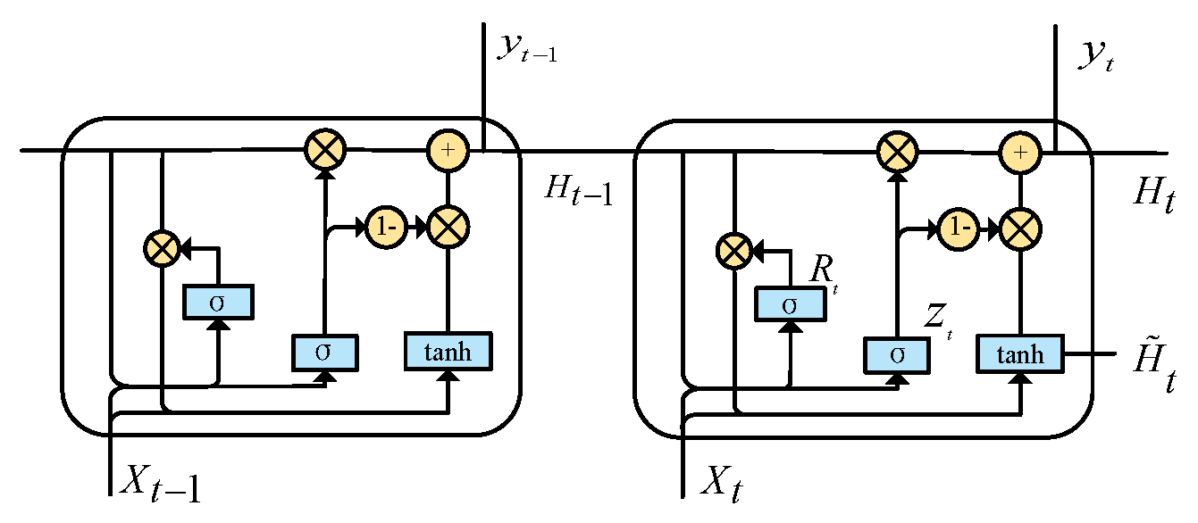
3.3. Gated Recurrent Unit

The gated recurrent unit (GRU) is a variant of recurrent neural networks (RNNs). Indeed, RNNs have been widely applied to model sequential data since their inception. In this paper, GRU is employed to process the TCN outputs, aiming to further capture the long-term dependencies within the data and enhance the accuracy of RUL predictions.

Steps (4)–(7) show the calculation process. $R_t$ represents the reset gate, which controls the retention of information from the previous time step. $Z_t$ represents the update gate, which controls the fusion of information. $\widetilde{H_t}$ represents the candidate hidden state at time t. Finally, the hidden states and outputs of the GRU are obtained by combining the update gate outputs and the candidate hidden states in (7).

$$\begin{array}{cc}\hfill R_t& =\sigma (W_{reset}·[H_{t-1},x_t]+b_{reset})\hfill \end{array}$$

(4)

$$\begin{array}{cc}\hfill Z_t& =\sigma (W_{update}·[H_{t-1},X_t]+b_{update})\hfill \end{array}$$

(5)

$$\begin{array}{cc}\hfill {\tilde{H}}_t& =tanh(W_{hid}·[R_t\odot H_{t-1},X_t]+b_{hid})\hfill \end{array}$$

(6)

$$\begin{array}{cc}\hfill H_t& =Z_t\odot H_{t-1}+(1-Z_t)\odot {\tilde{H}}_t\hfill \end{array}$$

(7)

Here, $\sigma$ is a sigmoid function, $W_{hid},W_{reset},W_{update}$ are the weights matrices, tanh is the hyperbolic tangent activation function, and $b_{update},b_{reset},b_{hid}$ are bias. For GRU, reset gates focus on short-term dependencies, while update gates handle long-term dependencies in sequences. Its structure is illustrated in Figure 3. Specifically, the reset and update gates transform the data into the range (0, 1) using a sigmoid function (4) and (5). Subsequently, the hidden state of the GRU is regulated by these two gates (6) and (7).

3.4. Proposed Methodology

The framework proposed is depicted in Figure 4. It comprises three components: data pre-processing, a TCN network integrated with an attention mechanism for feature extraction, and a GRU network for RUL prediction.

Data pre-processing involves feature selection, data normalization, and the generation of standardized training data using a sliding window approach. The next step involves defining the specific network architecture. First, the input data are aligned with the number of channels in the TCN through a fully connected layer. The TCN network captures deep-level features from the sensor sequence data. Next, an attention mechanism is applied to features across different time horizons to focus on key information that influences the RUL. Finally, the GRU network extracts cross-sensor information related to aero-engine performance degradation from the multi-temporally fused features.

In summary, the proposed neural network consists of MCA-TCN and GRU. The aero-engine sensor data are first processed by a modified TCN network to extract relevant features, which are then fed into the GRU network to obtain the predicted RUL value.

4. Experiment and Discussion

4.1. CMAPSS Datasets Description

CMAPSS is a dynamic, nonlinear, component-level model of a turbofan engine. From this model, NASA adjusted the input to create the CMAPSS dataset [33]. Specifically, this dataset is composed of four different sub-datasets. Each dataset can be split into a training set and a test set. The training set includes data from the full cycles of multiple aero-engines that degrade progressively until the RUL is zero, while the data from the test set end a certain cycle before the RUL is reduced to 0, and this RUL value is given in a separate file. At the same time, for different engine units in the dataset, there are different initial wear and tear conditions. The dataset’s basic information is presented in

Table 1. CMAPSS sub-datasets.

Sub-Datasets	FD001	FD002	FD003	FD004
train engines	100	260	100	249
test engines	100	259	100	248
conditions	1	6	1	6
failure model	1	1	2	2
Minimum RC	31	21	38	19

, where minimum RC stands for the shortest cycle time provided in the test datasets.

For each piece of data in the datasets, it consists of 21 sensor-recorded variables located at different locations in the aero-engine and 3 variables describing the operating conditions. Operating conditions include TRA, Mach number, and altitude. For FD001 and FD003, the data were generated under one operating condition, whereas the data for FD002 and FD004 were generated under six different operating conditions. The basic information of the 21 sensor variables is shown in

Table 2. Explanation of sensor variables.

Sensor Variables	Units	Description
T2	°R	Total temperature at fan inlet
T24	°R	Total temperature at LPC outlet
T30	°R	Total temperature at HPC outlet
P2	psia	Pressure at fan inlet
T50	°R	Total temperature at LPT outlet
Nf	rpm	Physical fan speed
P15	psia	Total pressure in bypass-duct
P30	psia	Total pressure at HPC outlet
Nc	rpm	Physical core speed
epr	–	Engine pressure ratio (P50/P2)
BPR	–	Bypass Ratio
farB	–	Burner fuel-air ratio
htBleed	–	Bleed Enthalpy
Ps30	psia	Static pressure at HPC outlet
phi	pps/psi	Ratio of fuel flow to Ps30
NRf	rpm	Corrected fan speed
NRc	rpm	Corrected core spee
Nf_dmd	rpm	Demanded fan speed
PCNfR_dmd	rpm	Demanded corrected fan speed
W31	lbm/s	HPT coolant bleed
W32	lbm/s	LPT coolant bleed

. Obviously, different sensors record distinct physical information, such as temperature, pressure, etc. Therefore, data pre-processing is essential to further enhance the model’s accuracy.

4.2. Data Pre-Processing

Within the datasets, sensor features have different scales, and when modeled directly by the framework, the effect of features with smaller values on the results would be ignored. For the neural network to achieve higher accuracy, data pre-processing is indispensable. The following section describes the necessary methods.

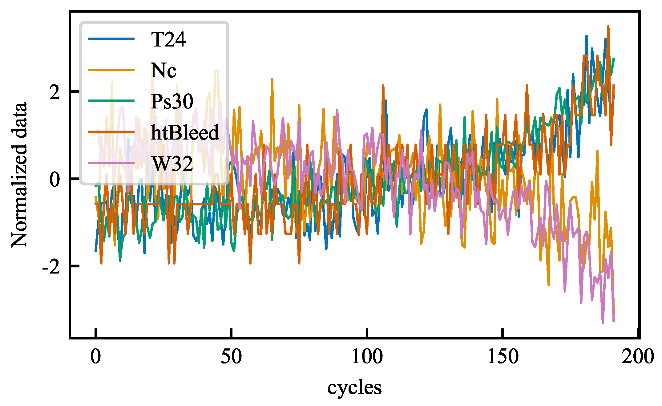
4.2.1. Z-Score Normalization

The data contained within the dataset exhibit varying scales, a factor that has a negative impact on the training process associated with the neural network. Consequently, a generalized normalization approach is used to normalize each feature variable separately. The sensor data can be transformed into normalized data with a mean of 0 and a variance of 1, so that the different sensor values are kept at a similar scale, as shown in Figure 5.

$$x_{norm}={\displaystyle \frac{x_i-\overline{x}}{\sigma }}$$

(8)

Here, $\overline{x}$ represents the mean of the input data, and $\sigma$ represents the data’s standard deviation.

Then, since some sensor values remain constant at a fixed value during performance degradation, this is redundant for the inputs to the neural network. Fourteen of these sensor features (sensors 2, 3, 4, 7, 8, 9, 11, 12, 13, 14, 15, 17, 20, 21) were selected for modeling.

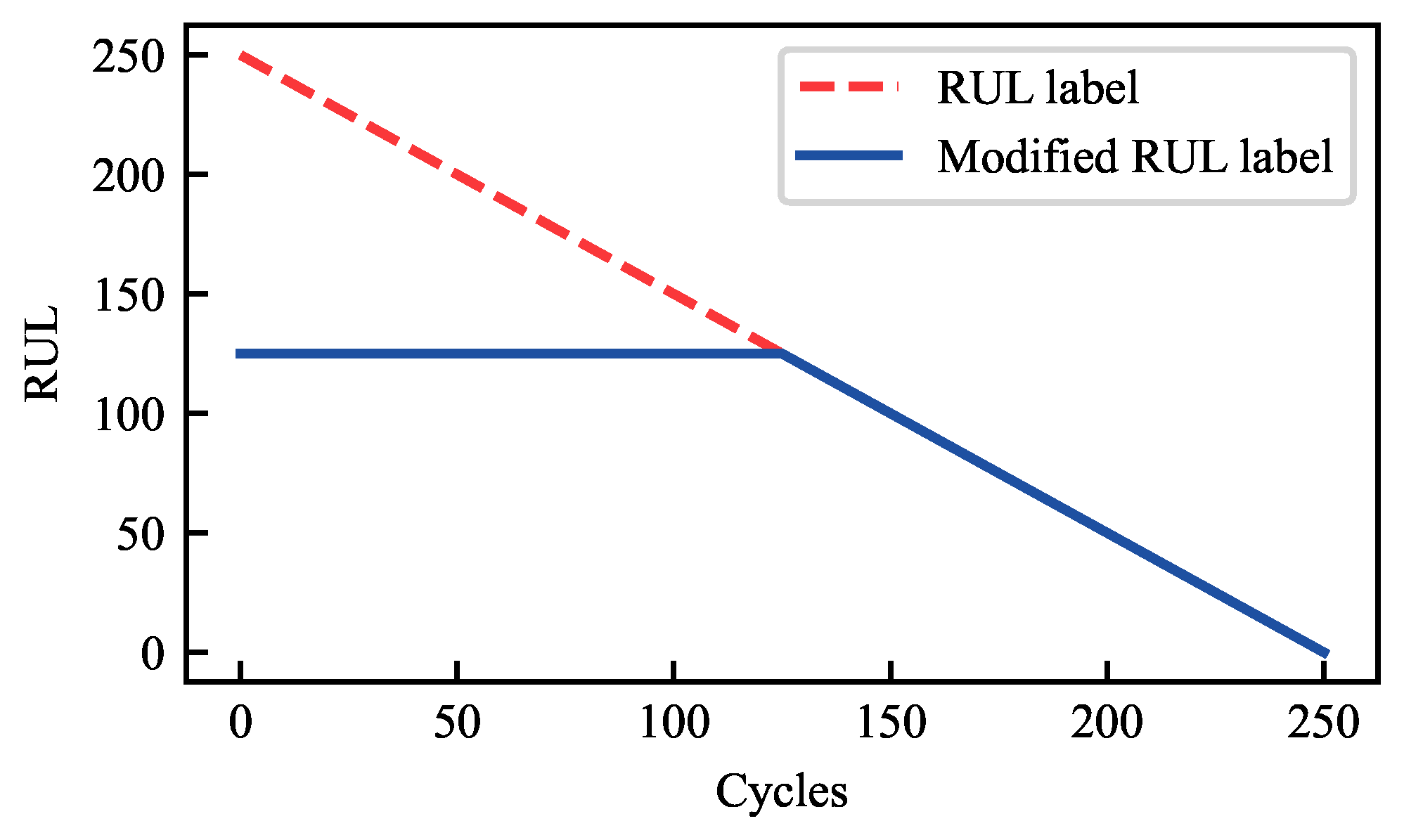
4.2.2. Two-Stage Degradation

In neural network backpropagation, model outputs and real labels are necessary to update the parameters of the model. To ensure that the proposed model fits the data better, from the trend of the data, it can be observed that for an engine, the parameter degradation occurs in two stages. In the first stage, the sensor-recorded values of the aero-engine decrease slowly with a small change. In the second stage, the change is more obvious. The threshold between the two stages is typically set to 125 [34]. Consequently, the value of RUL is converted to a two-stage representation, as illustrated in Figure 6. The data yielded by this method will be employed as labels for the training set.

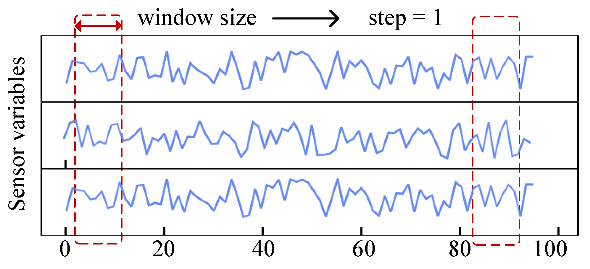
4.2.3. Sliding Window

For a single piece of data that only contains the measurements at the current moment, it is challenging for the model to extract information about performance degradation. To consider the effect of historical data and improve the model’s accuracy, the dataset is required to be processed through a sliding window. As shown in Figure 7, following a time window of sampling at a step size of 1 (the length of each forward step), the input data to the model is transformed into $({\mathbf{X}}_{train},y_{train})$, where $\mathbf{X}\in {\mathbb{R}}^{T\times d}$ (T is the size of sliding time window, d is the input data dimension), $y\in \mathbb{R}$. For instance, in the case of the engine shown in Figure 5, which consists of 192 cycles, a total of 173 training samples are obtained by applying a sliding window of size 30. The label for each sample is defined as the final RUL value within the original data window. The sliding window size has been demonstrated to affect input dimensions and model training; the impact on prediction performance will be analyzed using experiments.

4.3. Model Evaluation

To evaluate the network’s results and draw comparisons with other models, two approaches were utilized to calculate the prediction performance of the models, as follows.

4.3.1. Root Mean Square Error

To assess the accuracy of the predicted results against the actual data, the root mean square error (RMSE) is employed as a metric to evaluate the performance of the model and is usually calculated by the following (9):

$$\mathrm{RMSE}=\sqrt{{\displaystyle \frac{1}{N}}\sum _{i=1}^N{(y_i-{\widehat{y}}_i)}^2}$$

(9)

4.3.2. Score Function

In a PHM challenge, the model’s predictions are evaluated with the following equation. Compared to the RMSE, this calculation gives a larger penalty score for overly optimistic forecasting results.

$$score=\left\{\begin{array}{cc}{\sum }_{i=1}^N(e^{-{\displaystyle \frac{{\widehat{y}}_i-y_i}{13}}}-1),\hfill & \mathrm{if}{\widehat{y}}_i<y_i\hfill \\ {\sum }_{i=1}^N(e^{{\displaystyle \frac{{\widehat{y}}_i-y_i}{10}}}-1),\hfill & \mathrm{if}{\widehat{y}}_i\ge y_i.\hfill \end{array}\right.$$

(10)

Here, n represents the number of samples in the test set, $y_i$ denotes the actual RUL value of the input data, and ${\widehat{y}}_i$ refers to the predicted value from the model’s output.

4.4. Experimental Setup

The grid search method was selected for investigating the impact of various parameter variations on the prediction accuracy of the model, allowing for the identification of the optimal hyperparameters. Specifically, a predefined set of values is assigned to each hyperparameter. In each experiment, one value from each set is selected to form the hyperparameter configuration. The hyperparameter set is also based on experience and references. For example, the TCN channel searches from [15, 20, 15, 30], the batch size searches from [128, 256, 512, 1024]. The MSE loss function is to be employed during the training of the neural network. The Adam optimizer is chosen to optimize parameters of the network, where the learning rate decreases gradually with the increase of epoch, which is multiplied by 0.9 every 10 epochs. The obtained optimal hyperparameters are presented in

Table 3. Default hyperparameters of the model.

Hyperparameter	Descriptions	Value
Batch size	Samples per update step	512
Epoch	Complete training cycles	60
Lr	Initial learning rate	0.001
Dropout rate	The proportion of neurons randomly deactivated	0.25
TCN channels	The number of channels in one TCN block	20
TCN BLOCKS	The total number of TCN blocks	3
GRU size	The number of GRU units	18

. All experiments were performed on Windows 11, Python version 3.10, PyTorch framework 2.5.1, with NVIDIA 4060 GPU.

For the purpose of evaluating the generalization error of the model during training, 20% of the engine units were used in the training set as the validation set (a subset of the training set of the dataset is selected for validation, while the test set is kept unchanged). Furthermore, by observing the changes in the validation set error, it is possible to determine whether to adopt an early stopping strategy and evaluate the overfitting phenomenon.

4.5. Experimental Results

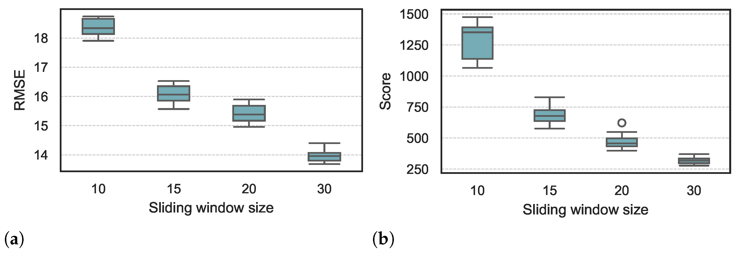
4.5.1. The Effect of Sliding Time Windows

The FD001 dataset was selected for this experiment. Sliding time windows of different sizes were applied to the FD001 dataset to obtain the RMSE and evaluation scores.

In the case of the CMAPSS dataset, a single record of data is representative of one duty cycle of the engine. Degradation of components is an inherently gradual process. The size of the sliding window, therefore, is the key factor in determining the amount of information that can be obtained. An increased sliding window consequently provides greater degradation information for a past time period. As shown in Table 2, the lowest number of cycles for the FD001 test set is 31. For this reason, four sizes (10, 15, 20, and 30) were selected for the experiment.

Within each sliding window size, the experiment was carried out ten times to assure the stability of the experiment results. The result is shown in Figure 8. It is evident that as the length of the window increases, both the RMSE and the score of the RUL predicted values demonstrate a decreasing trend. When the window size is set at 10, the RMSE generally falls in the 18 to 19 range. Furthermore, as the window size increases, the results have been observed to drop below 14.

4.5.2. Ablation Experiments of the Proposed Method

In this part, the attention module of the proposed framework is removed from the neural network. In effect, the pre-processing of the data remains the same, and the model is instead modified to simply output with a combination of TCN and GRU layers. Thus, two models are obtained: TCN-GRU and TCN with Attention-GRU. The FD002 and FD004 datasets are selected for ablation experiments. The results are shown in

Table 4. Performance comparison with and without attention structure.

Methods	FD002		FD004
	RMSE	Score	RMSE	Score
Without attention	16.72	1361.8	20.50	3502.93
With attention	16.19	1189.4	18.33	2091.27

. By analyzing the results, it is shown that the TCN network with an attention mechanism can obtain higher prediction accuracy. Furthermore, the TCN network employs an attention mechanism that enables the capture of valid information from the input data. This information can then be blended and provided to the GRU for the prediction of RUL. As displayed in Figure 9, the weights calculated by the attention framework at the testing stage are presented.

4.5.3. Comparison of the Proposed Methodology with Previous Methodologies

In this segment, the proposed method’s accuracy is compared with other RUL prediction methods. The FD002 and FD004 sub-datasets from the CMAPSS dataset are chosen for analysis in this study.

Figure 10 shows the results of predicting the RUL against the real values for all engines in the datasets. Meanwhile, the error distribution of the prediction errors for all engine units was plotted. Moreover, Figure 11 presents the complete cycle prediction results for a specific engine unit in the datasets. The comparison with other methods in RMSE of the predicted results is presented in

Table 5. Performance comparison with other methods.

Methods	Year	FD002		FD004
		RMSE	Score	RMSE	Score
DCNN [20]	2018	24.86	\	29.44	\
Dt-LSTM [35]	2019	17.87	\	21.81	\
AGCNN [28]	2020	19.43	1492	21.50	3392
MS-DCNN [21]	2020	19.35	3747	22.22	4844
MSDCNN-LSTM [36]	2023	18.70	1873.86	21.57	2699.34
MSIDSN [37]	2023	18.26	2046.65	22.48	2910.73
CATA-TCN [27]	2024	17.61	1361.23	21.04	2303.42
proposed model	-	16.19	1189.4	18.33	2091.27

“\” represents data not given by the authors.

, where the RMSE is computed based on all predictions shown in Figure 10.

4.6. Discussion

In the experimental section, repeated experiments are conducted on the FD001 dataset by adjusting the sliding window size to verify the hypothesis that a larger window provides more effective information and enhances prediction accuracy. Secondly, the efficacy of the designed multichannel attention mechanism was validated through ablation experiments. Clearly, the attention computed towards the TCN block input channels enables the model to attend to potential information. Consequently, there is an observed decline in RMSE and evaluation scores on FD002 and FD004. Finally, the model’s performance was validated on the FD002 and FD004 datasets.

In Table 5, the proposed method was compared with previously introduced approaches in other studies. Some models have been selected from the last few years that include DCNN [20], Dt-LSTM [35], AGCNN [28], MS-DCNN [21], MSDCNN-LSTM [21], MSIDSN [37], and CATA-TCN [27]. These models are based on studies carried out in recent years. Their key messages are outlined in

Table 6. Performance comparison with other methods.

Methods	Main Contributions
DCNN	A deep convolutional network without prior knowledge and signal processing
Dt-LSTM	Proposes a dual-task deep LSTM network
AGCNN	An attention mechanism that dynamically adjusts weights
MS-DCNN	A multi-scale deep convolutional network
MSDCNN-LSTM	Combines deep convolutional networks and LSTM networks
MSIDSN	Self-attentive mechanism and parallel BiGRU to improve prediction performance
CATA-TCN	Combination of channel and temporal attention to capture key information
Proposed model	Proposing a novel attention mechanism for fusing multilayer networks

. The experimental results confirm that the proposed model achieves higher efficiency in estimating the remaining useful life of the engine on the FD002 and FD004 datasets, exhibiting superior accuracy in both RMSE and evaluation metrics.

Despite the improvements achieved by the proposed model in terms of RMSE, the predicted values still exhibit severe deviations, as shown in Figure 10. Moreover, the comparison with models from other studies does not demonstrate substantial advancements. Additionally, the generalizability of the proposed model to the remaining dataset has not been validated, which will be a key focus of future research.

5. Conclusions

An advanced framework for predicting remaining useful life is introduced in this article, comprising two key components: a temporal convolutional network with multichannel attention and a gated recurrent unit network. After pre-processing the dataset, the data are initially processed through an overlaying TCN network, followed by the fusion of multiple TCN blocks using our proposed attention-based computation approach. Finally, the processed data are passed through the GRU network to generate RUL predictions. It has been established through experiments on the CMAPSS dataset that our proposed TCN channels attention computation can effectively improve accuracy.

Despite the contributions of our work, there are some limitations. For example, the model’s generalizability to other datasets requires further enhancement, and there is still potential to improve its predictive performance. Future work will enhance the generalization of the model further, validate it on more datasets, and further improve the structure of the model.

References

1. Dangut, M.D.; Jennions, I.K.; King, S.; Skaf, Z. Application of deep reinforcement learning for extremely rare failure prediction in aircraft maintenance. Mech. Syst. Signal Process. 2022, 171, 108873. [Google Scholar] [CrossRef]
2. Ren, H.; Chen, X.; Chen, Y. Reliability Based Aircraft Maintenance Optimization and Applications; Academic Press: Cambridge, MA, USA, 2017. [Google Scholar]
3. Kordestani, M.; Orchard, M.E.; Khorasani, K.; Saif, M. An overview of the state of the art in aircraft prognostic and health management strategies. IEEE Trans. Instrum. Meas. 2023, 72, 3505215. [Google Scholar] [CrossRef]
4. De Pater, I.; Reijns, A.; Mitici, M. Alarm-based predictive maintenance scheduling for aircraft engines with imperfect Remaining Useful Life prognostics. Reliab. Eng. Syst. Saf. 2022, 221, 108341. [Google Scholar]
5. Ordóñez, C.; Lasheras, F.S.; Roca-Pardiñas, J.; de Cos Juez, F.J. A hybrid ARIMA–SVM model for the study of the remaining useful life of aircraft engines. J. Comput. Appl. Math. 2019, 346, 184–191. [Google Scholar]
6. Dong, R.; Li, W.; Ai, F.; Wan, M. Design of PHM test verification method and system for aviation electrical system. In Proceedings of the 2021 Global Reliability and Prognostics and Health Management (PHM-Nanjing), Nanjing, China, 15–17 October 2021; pp. 1–5. [Google Scholar]
7. Raouf, I.; Kumar, P.; Cheon, Y.; Tanveer, M.; Jo, S.H.; Kim, H.S. Advances in prognostics and health management for aircraft landing gear—progress, challenges, and future possibilities. Int. J. Precis. Eng. Manuf.-Green Technol. 2025, 12, 301–320. [Google Scholar]
8. Li, C.; Li, S.; Feng, Y.; Gryllias, K.; Gu, F.; Pecht, M. Small data challenges for intelligent prognostics and health management: A review. Artif. Intell. Rev. 2024, 57, 214. [Google Scholar] [CrossRef]
9. Zio, E. Prognostics and Health Management (PHM): Where are we and where do we (need to) go in theory and practice. Reliab. Eng. Syst. Saf. 2022, 218, 108119. [Google Scholar]
10. Zhang, Y.; Fang, L.; Qi, Z.; Deng, H. A review of remaining useful life prediction approaches for mechanical equipment. IEEE Sens. J. 2023, 23, 29991–30006. [Google Scholar]
11. Hesabi, H.; Nourelfath, M.; Hajji, A. A deep learning predictive model for selective maintenance optimization. Reliab. Eng. Syst. Saf. 2022, 219, 108191. [Google Scholar] [CrossRef]
12. Deepika, J.; Reddy, P.M.; Murari, K.; Rahul, B. Predictive Maintenance of Aircraft Engines: Machine Learning Approaches for Remaining Useful Life Estimation. In Proceedings of the 2025 6th International Conference on Mobile Computing and Sustainable Informatics (ICMCSI), Morang, Nepal, 7–8 January 2025; pp. 1679–1686. [Google Scholar]
13. Dangut, M.D.; Skaf, Z.; Jennions, I.K. Handling imbalanced data for aircraft predictive maintenance using the BACHE algorithm. Appl. Soft Comput. 2022, 123, 108924. [Google Scholar]
14. Jia, W.; Haimin, L.; Xiao, W. Application and design of PHM in aircraft’s integrated modular mission system. In Proceedings of the 2019 Prognostics and System Health Management Conference (PHM-Qingdao), Qingdao, China, 25–27 October 2019; pp. 1–6. [Google Scholar]
15. Kiakojoori, S.; Khorasani, K. Dynamic neural networks for gas turbine engine degradation prediction, health monitoring and prognosis. Neural Comput. Appl. 2016, 27, 2157–2192. [Google Scholar]
16. Zhou, H.; Zhang, S.; Peng, J.; Zhang, S.; Li, J.; Xiong, H.; Zhang, W. Informer: Beyond efficient transformer for long sequence time-series forecasting. In Proceedings of the AAAI Conference on Artificial Intelligence, virtually, 2–9 February 2021; Volume 35, pp. 11106–11115. [Google Scholar]
17. Fang, X.; Xie, L.; Dimarogonas, D.V. Simultaneous distributed localization and formation tracking control via matrix-weighted position constraints. Automatica 2025, 175, 112188. [Google Scholar]
18. El-Brawany, M.A.; Ibrahim, D.A.; Elminir, H.K.; Elattar, H.M.; Ramadan, E. Artificial intelligence-based data-driven prognostics in industry: A survey. Comput. Ind. Eng. 2023, 184, 109605. [Google Scholar] [CrossRef]
19. Gawde, S.; Patil, S.; Kumar, S.; Kamat, P.; Kotecha, K.; Abraham, A. Multi-fault diagnosis of Industrial Rotating Machines using Data-driven approach: A review of two decades of research. Eng. Appl. Artif. Intell. 2023, 123, 106139. [Google Scholar]
20. Li, X.; Ding, Q.; Sun, J.Q. Remaining useful life estimation in prognostics using deep convolution neural networks. Reliab. Eng. Syst. Saf. 2018, 172, 1–11. [Google Scholar]
21. Li, H.; Zhao, W.; Zhang, Y.; Zio, E. Remaining useful life prediction using multi-scale deep convolutional neural network. Appl. Soft Comput. 2020, 89, 106113. [Google Scholar]
22. Shi, Z.; Chehade, A. A dual-LSTM framework combining change point detection and remaining useful life prediction. Reliab. Eng. Syst. Saf. 2021, 205, 107257. [Google Scholar]
23. Yan, J.; He, Z.; He, S. Multitask learning of health state assessment and remaining useful life prediction for sensor-equipped machines. Reliab. Eng. Syst. Saf. 2023, 234, 109141. [Google Scholar] [CrossRef]
24. Li, H.; Li, Y.; Wang, Z.; Li, Z. Remaining useful life prediction of aero-engine based on PCA-LSTM. In Proceedings of the 2021 7th International Conference on Condition Monitoring of Machinery in Non-Stationary Operations (CMMNO), Guangzhou, China, 11–13 June 2021; pp. 63–66. [Google Scholar]
25. Woo, S.; Park, J.; Lee, J.Y.; Kweon, I.S. Cbam: Convolutional block attention module. In Proceedings of the European Conference on Computer Vision (ECCV), Munich, Germany, 8–14 September 2018; pp. 3–19. [Google Scholar]
26. Hu, J.; Shen, L.; Sun, G. Squeeze-and-excitation networks. In Proceedings of the IEEE Conference on Computer Vision and Pattern Recognition, Salt Lake City, UT, USA, 18–23 June 2018; pp. 7132–7141. [Google Scholar]
27. Lin, L.; Wu, J.; Fu, S.; Zhang, S.; Tong, C.; Zu, L. Channel attention & temporal attention based temporal convolutional network: A dual attention framework for remaining useful life prediction of the aircraft engines. Adv. Eng. Inform. 2024, 60, 102372. [Google Scholar]
28. Liu, H.; Liu, Z.; Jia, W.; Lin, X. Remaining useful life prediction using a novel feature-attention-based end-to-end approach. IEEE Trans. Ind. Inform. 2020, 17, 1197–1207. [Google Scholar] [CrossRef]
29. Li, L.; Li, Y.; Mao, R.; Li, Y.; Lu, W.; Zhang, J. TPANet: A novel triple parallel attention network approach for remaining useful life prediction of lithium-ion batteries. Energy 2024, 309, 132890. [Google Scholar] [CrossRef]
30. Bai, S.; Kolter, J.Z.; Koltun, V. An empirical evaluation of generic convolutional and recurrent networks for sequence modeling. arXiv 2018, arXiv:1803.01271. [Google Scholar]
31. He, K.; Zhang, X.; Ren, S.; Sun, J. Deep residual learning for image recognition. In Proceedings of the IEEE Conference on Computer Vision and Pattern Recognition, Las Vegas, NV, USA, 27–30 June 2016; pp. 770–778. [Google Scholar]
32. Wang, Q.; Wu, B.; Zhu, P.; Li, P.; Zuo, W.; Hu, Q. ECA-Net: Efficient channel attention for deep convolutional neural networks. In Proceedings of the IEEE/CVF Conference on Computer Vision and Pattern Recognition, Seattle, WA, USA, 13–19 June 2020; pp. 11534–11542. [Google Scholar]
33. Saxena, A.; Goebel, K.; Simon, D.; Eklund, N. Damage propagation modeling for aircraft engine run-to-failure simulation. In Proceedings of the 2008 International Conference on Prognostics and Health Management, Denver, CO, USA, 6–9 October 2008; pp. 1–9. [Google Scholar]
34. Heimes, F.O. Recurrent neural networks for remaining useful life estimation. In Proceedings of the 2008 International Conference on Prognostics and Health Management, Denver, CO, USA, 6–9 October 2008; pp. 1–6. [Google Scholar]
35. Miao, H.; Li, B.; Sun, C.; Liu, J. Joint learning of degradation assessment and RUL prediction for aeroengines via dual-task deep LSTM networks. IEEE Trans. Ind. Inform. 2019, 15, 5023–5032. [Google Scholar] [CrossRef]
36. Chen, W.; Liu, C.; Chen, Q.; Wu, P. Multi-scale memory-enhanced method for predicting the remaining useful life of aircraft engines. Neural Comput. Appl. 2023, 35, 2225–2241. [Google Scholar] [CrossRef]
37. Zhao, K.; Jia, Z.; Jia, F.; Shao, H. Multi-scale integrated deep self-attention network for predicting remaining useful life of aero-engine. Eng. Appl. Artif. Intell. 2023, 120, 105860. [Google Scholar] [CrossRef]
Figure 1. Two key structures in TCN. (a) Dilated Convolutional Structure. (b) Residual Connection Block.
Energies 18 01899 g001
Figure 2. Method for calculating attention weights of TCN channels at different levels.
Energies 18 01899 g002
Figure 3. Structure of the GRU unit.
Energies 18 01899 g003
Figure 4. The proposed network structure.
Energies 18 01899 g004
Figure 5. Some normalized sensor data from engine #1 in training set FD001.
Energies 18 01899 g005
Figure 6. RUL two-stage degradation.
Energies 18 01899 g006
Figure 7. Sliding window method.
Energies 18 01899 g007
Figure 8. Evaluation results for the FD001 test set vs. window size. (a) RMSE results of different window sizes. (b) Score results of different window sizes.
Energies 18 01899 g008
Figure 9. The result of an attention calculation at some point during the test (Weights for adjusting the importance of channels across multiple TCN blocks).
Energies 18 01899 g009
Figure 10. Model prediction results for FD002 and FD004 (The real RUL represents the RUL given in the dataset, and the predicted RUL represents the predicted value of the model). (a) FD002. (b) FD004. (c) Error distribution of FD002. (d) Error distribution of FD004.
Energies 18 01899 g010
Figure 11. Predicted results for a unit in the test set. (a) FD002 #235 Engine. (b) FD004 #110 Engine.
Energies 18 01899 g011