Article

Model-Free Adaptive Fuzzy Sliding-Mode Observer Control for PMSM

School of Electrical and Information Engineering, Jiangsu University, Zhenjiang 212013, China
*
Author to whom correspondence should be addressed.
Energies 2025, 18(8), 1877; https://doi.org/10.3390/en18081877
Submission received: 26 February 2025 / Revised: 4 April 2025 / Accepted: 5 April 2025 / Published: 8 April 2025
(This article belongs to the Special Issue Measurement Systems for Electric Machines and Motor Drives)

Abstract

:
To further improve the estimation accuracy of the super-spiral observer, this paper innovatively proposes a fuzzy model-free adaptive control (FMFAC) super-spiral observer. The control scheme exhibits improved estimation accuracy after incorporating a fuzzy model-free adaptive component. The main contributions of this paper are as follows: (1) to achieve comprehensive fuzzy parameters without model adaptation, and (2) to creatively summarize the fuzzy rule table according to the observer’s characteristics. Experimental results demonstrate that the control performance of the proposed observer surpasses that of the traditional hyper-spiral observer.

1. Introduction

Due to their excellent robustness, sliding-mode observers are widely used in various control systems [1,2,3]. However, traditional sliding-mode observers often suffer from chattering, which can affect estimation performance [4]. To address this issue, References [5,6] proposed using new functions to replace the sign function, thereby enhancing system performance. Additionally, Reference [7] introduced an adaptive super-twisting sliding-mode observer that updates in real time based on the system speed; this method is used for sensorless control. Reference [8] proposed a sliding-mode speed controller based on a novel reaching law. In Reference [9], an adaptive approach rate was designed to solve the contradiction between the approach times of traditional sliding-mode observers and system buffeting. Reference [10] employed a continuous saturation function instead of a discontinuous switching function to minimize buffeting error. Reference [11] replaced fixed sliding-mode gain with a variable reaching rate to obtain accurate information on rotor position and velocity. References [12,13] utilized fuzzy control to adjust the sliding-mode gain, thereby reducing the observation error. In Reference [14], a second-order generalized integrator is used for notch processing of non-fundamental signals, preserving the fundamental information of the back electromotive force. Reference [15] proposed an adaptive gain hyper-torsional sliding-mode observer, which utilizes the adaptive gain value in the control law of the Lyapunov stability theory to enhance the robustness of the motor parameters against deviations. Reference [16] employed a new continuous function, T(s), instead of a symbolic function to mitigate buffeting. These developments are designed to meet the practical application requirements of PMSMs.
To address the issue of estimation accuracy of the super-spiral observer, a fuzzy model-free adaptive super-spiral observer is proposed. The contributions of this paper are summarized as follows:
  • In the realm of model-free adaptive control (MFAC), the general rules for parameter adjustment are given. The four parameters of model-free adaptive control are adjusted online, and two improvement schemes are proposed, namely, enhancing the MFAC input signal to improve the universality of the control, and refining the pseudo-bias reset to mitigate interference caused by false resets.
  • Fuzzy model-free adaptive control is applied to the observer of the permanent magnet synchronous motor; the fuzzy rule table is explicitly summarized to compensate for the superhelix observer’s error, addressing the problem of the error rate of change being too fast. This approach ensures accurate estimation of the back electromotive force. The process and reasons for parameter adjustments are given and explained in detail, providing a theoretical foundation for the application of fuzzy model-free adaptive control.
Reference [4] proposed an adaptive push-back sliding-mode control with a nonlinear disturbance observer, the core of which is the use of push-back control. The advantage is that parameter uncertainty and external load torque perturbations can be observed. However, there are too many control parameters, which makes it difficult to control. In Reference [17], a generalized high-order observer was proposed to estimate the total disturbance in a permanent magnet synchronous motor (PMSM), the core of which involves the use of an order state observer. This method is relatively robust; however, its design and implementation are complicated and require superior hardware. References [18,19,20,21] combined neural networks with existing techniques to improve the estimation accuracy of observers. However, neural network control exhibits weak fault tolerance, requires longer training times, and presents more difficult debugging challenges.
Compared to other online parameter-tuning technologies—although the optimal controller gain comparable to that of traditional model-free adaptive control can be obtained in References [22,23]—a fuzzy model-free adaptive control adjusts the gain through two dimensions, namely, fuzzification and pseudo-partial derivative. Higher control accuracy is achievable. Neural network learning control can also achieve precise control; however, the training time is lengthy and may even result in training failure [24]. Hybrid learning approaches reach their optimal solution faster, but it is challenging to perform efficient operations over time [25]. Inverse reinforcement learning exhibits strong stability but poor robustness [26]. Machine learning can improve training efficiency, but the internal decision-making process is challenging to understand and explain [27,28]. Simultaneous perturbation stochastic approximation requires a large amount of computation and has a slow convergence rate [29]. The fuzzy model-free adaptive control has better control performance when the sliding-mode observer’s error range is extensive and the error change rate is large. In particular, the parameters can be adjusted sensitively in response to changes in the error rate to minimize the estimation error. This is also the most crucial reason for choosing fuzzy model-free adaptive control among many online controls.
The main difficulty in this paper lies in the numerous parameters of model-free adaptive control, as the pseudo-bias change is significantly influenced by the pseudo-bias reset, making the adjustment process challenging. After the introduction of fuzzy control, although control flexibility has been dramatically improved, more parameters have undoubtedly been added, which further complicates the adjustment process.
The research content of this paper is primarily divided into the following sections: Section 1 summarizes previous research, outlines the research content of this paper, and provides a comparison with existing studies. In Section 2, the fuzzy model-free adaptive observer is analyzed in detail, including the optimization of fuzzy parameters. In Section 3, simulation and experimental verifications are made for the research. Section 4 discusses the paper’s shortcomings and outlines future research directions.

2. Fuzzy Model-Free Adaptive Sliding-Mode Observer

2.1. Traditional MFAC

With ongoing development and improvement by scholars both domestically and internationally, MFAC has made significant progress in various fields, and it has also seen corresponding advancements in the domain of permanent magnet synchronous motor (PMSM) drive control.
MFAC is a dynamic linearization method used, which can be expressed as follows:
e m ( k ) = e m ( k 1 ) + ρ ϕ ^ ( k ) λ + | ϕ ^ ( k ) | 2 [ i * ( k + 1 ) i ( k ) ]
ϕ ^ c ( k ) = ϕ ^ c ( k 1 ) + η Δ e m ( k 1 ) μ + Δ e m ( k 1 ) 2 [ Δ i ( k ) ϕ ^ c ( k 1 ) Δ e m ( k 1 ) ]
When sign ( φ ^ c ( k ) ) sign ( φ ^ c ( 1 ) ) or φ ^ c ( k ) ε , we have the following:
ϕ ^ c ( k ) = ϕ ^ c ( 1 )
In the equation, i(k) and i*(k) represent the actual and estimated stator currents, respectively. φc(k) denotes the pseudo-partial derivative (PPD). em(k) denotes the model-free adaptive component of the back electromotive force. Λ > 0 denotes the weight factor, μ > 0 denotes the pseudo-partial derivative weight factor. ρ ∈ (0, 1] denotes the step size factor. η ∈ (0, 1] denotes the pseudo-partial derivative step size factor. Since the parameters of the PMSM are represented under the α-β axes, em(k), i(k), i*(k), and φc(k) are matrices corresponding to these parameters.
e m ( k ) = e m α ( k ) e m β ( k )
The flow diagram of MFAC is shown in Figure 1.

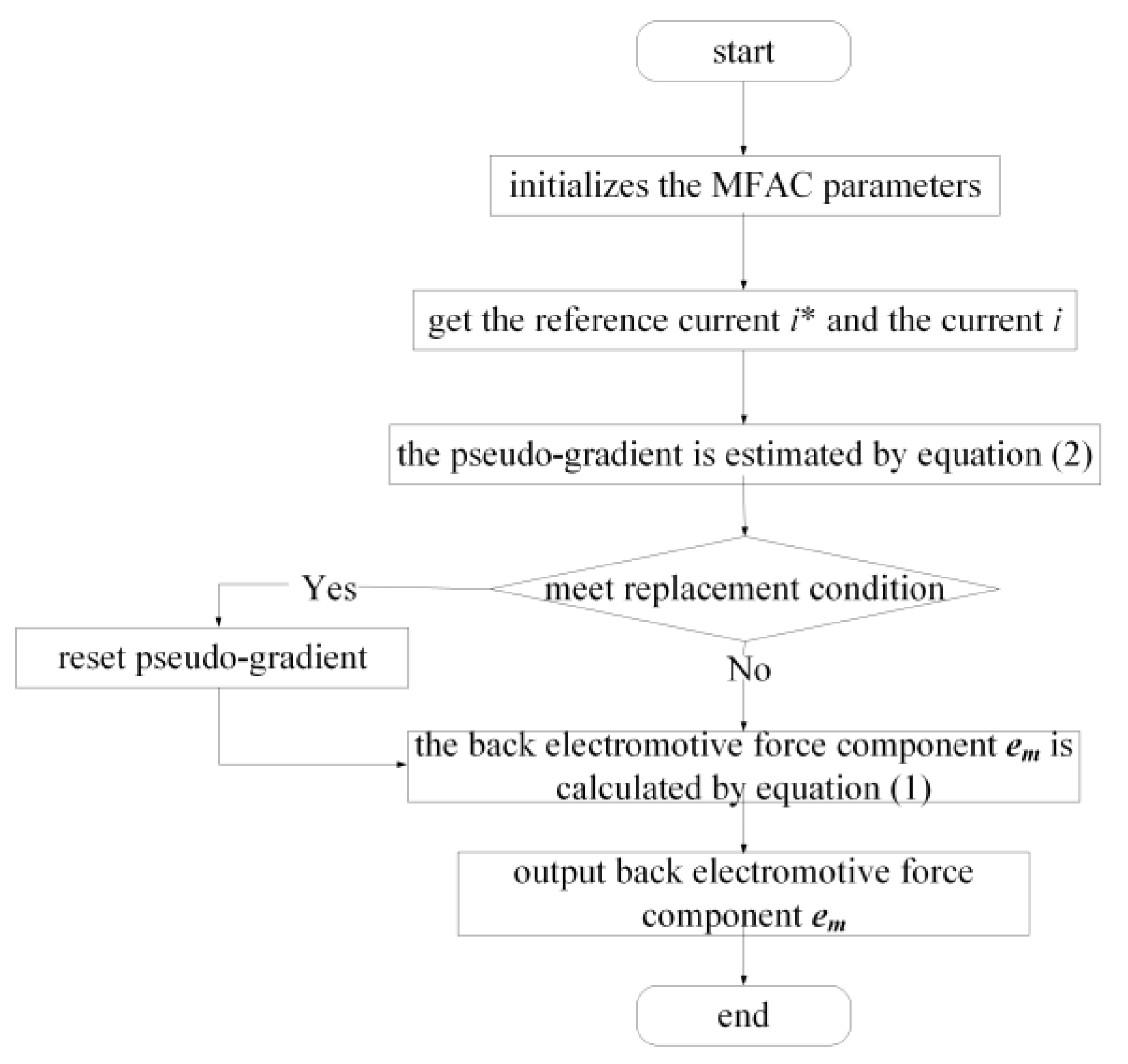
2.2. Based on the Improved MFAC Algorithm

In practical control, the narrow control range of ρ ∈ (0, 1] may lead to issues such as steady-state errors. To further enhance the range of model-free adaptive control and improve the general applicability of the control method, the following improvements are made to the input signal:
Q * ( k + 1 ) = i * ( k + 1 ) a Q ( k ) = i ( k ) a
Introducing a tunable constant greater than zero can significantly expand the applicability and design flexibility of MFAC, enabling it to handle more complex application scenarios. However, if constant a is too large, it may lead to steady-state errors, thereby affecting control performance. Conversely, if a is too small, it may increase overshoot and even lead to system instability.

2.3. Parameter-Tuning Method of MFAC in Sliding-Mode Observer

During the process of adjusting parameters in practice, since MFAC requires changes to a large number of parameters, a detailed description of the specific role of each parameter in PMSM is necessary. The parameters to be adjusted are as follows: Step factor ρ, weight factor λ, pseudo-bias step factor μ, pseudo-bias weight factor η, pseudo-bias initial value φc(1), pseudo-bias reset threshold ε, adjustable constant a, back electromotive force initial value e(0), stator current initial value i(0), i(1), etc. Due to the applications in various locations, specific parameters are adjusted to make corresponding changes by other systems.
The step factor ρ ∈ (0,1) functions similarly to the scale parameter P in PID control, except that the step factor ρ of MFAC and the initial value φc(1) of the pseudo-bias can jointly reflect the current deviation of the system. Increasing ρ can significantly improve the system’s rapidity and reduce the time to reach a steady state, setting ρ too high may lead to instability.
The weight factor λ > 0, λ is an essential means to suppress overshoot; its role is similar to the proportional parameter I in PID control, that is, λ is too large to reduce the response speed and reduce overshoot; if λ is too small, the response speed will increase, while the overshoot will increase. Lambda = 0 can destabilize.
The pseudo-biased step size factor μ and the pseudo-biased weight factor η are designed to change the derivative in real time based on the input and output changes. Their tuning method is closely related to φc(k), that is, the function of φc(k) is to automatically change into φc(k), which meets the stability of the system according to the I/O data of the system because the size of φc(k) is a parameter that changes according to the input and output; φc(k) is a slow time-varying parameter, and the change range is small, resulting in more minor changes in each cycle. The pseudo-bias weight factor η is a parameter used to reflect part of the current deviation of φc(k). If η is too small, the influence of φc(k) on the system will be reduced, and the rapidity will be reduced. If η is too small, the influence of φc(k) on the system will be increased. If the pseudo-bias step factor μ is too large, it can reduce the amplitude of variation in φc(k) and minimize overshoot. Still, the time to steady state will also increase, and it will be shorter when μ is too small; however, this makes it more prone to instability.
There are several similarities between the initial value φc(1) and the step factor ρ: increasing φc(1) can significantly enhance rapidity and reduce the time to reach a steady state. In contrast, excessively large φc(1) may lead to instability. The difference is that the original intention of the pseudo-partial derivative initial value φc(1) is to enhance the system’s updating ability, and φc(1) can reflect the strength of the algorithm’s recovery. Due to the high control requirements of PMSM and the low sampling frequency, there is no need to improve the updating ability after the steady state is reached, which will lead to multiple false triggers for the pseudo-bias reset. Therefore, setting φc(1) too large will produce significant steady-state errors and affect the steady-state performance.
The false bias reset threshold ε is a crucial parameter of the recovery algorithm, typically set to 1 × 10⁻⁵. When ε is small, the false bias reset becomes more challenging to achieve, and the algorithm’s ability to update becomes weaker. When ε increases, the false bias reset is easily accomplished; however, it also increases the frequency of false touches, thereby affecting performance.
The tunable constant a represents a further improvement to the problem, as the control range of the step factor ρ ∈ (0, 1) is too small. The scope and effect of regulation and control are increased.
The initial value of the back electromotive force e(0), the initial value of the stator current i(0), i(1), and other parameters are generally set to 0. However, suppose the steady-state and dynamic changes of the input and output of MFAC are too significant, and the change rate is not rapid. In this case, better dynamic performance can be achieved by adjusting e(0), i(0), and i(1).

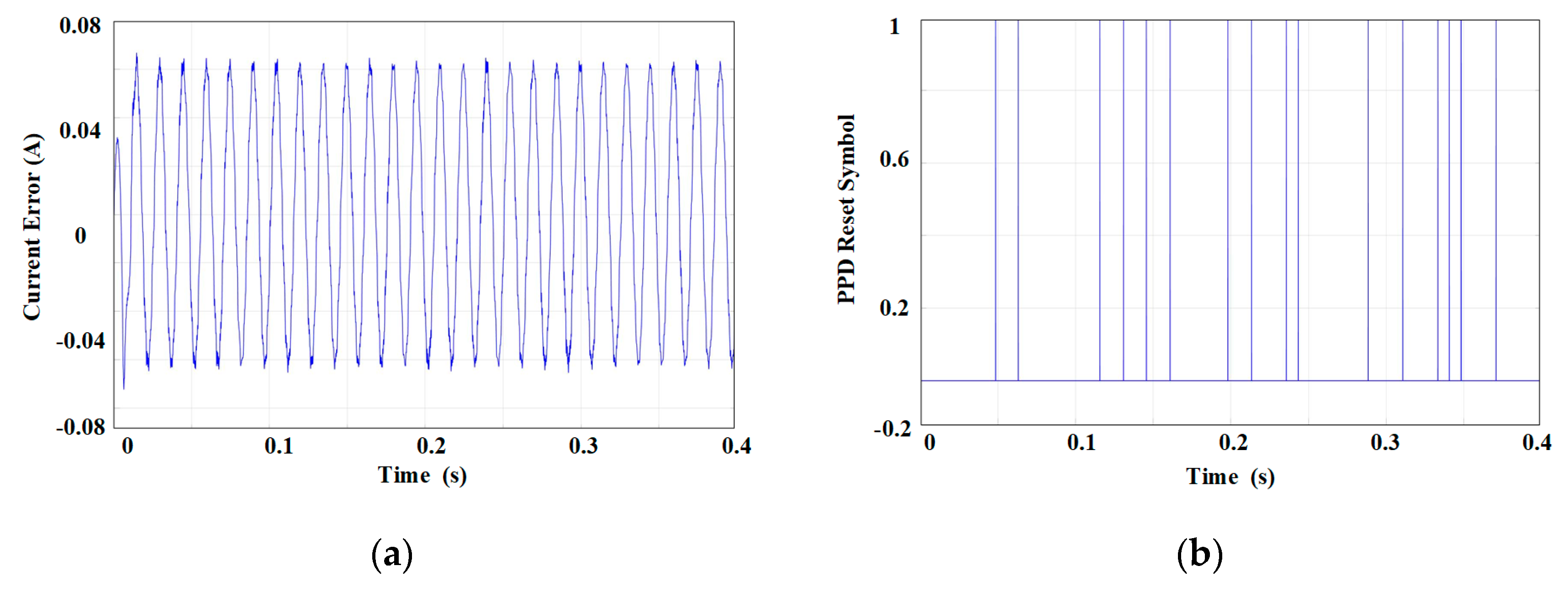
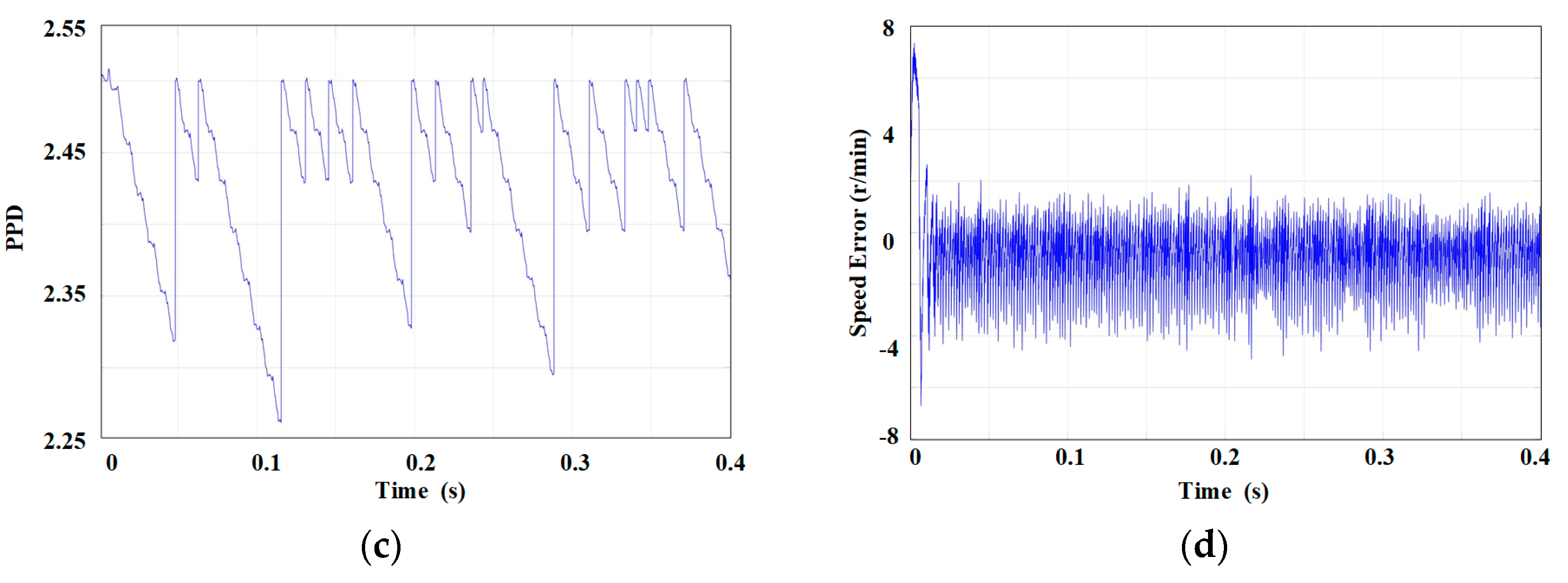
2.4. Based on the Improved PPD Reset Algorithm

The original intention of the PPD reset algorithm is to enhance the update capability of the algorithm when its gain weakens [29]. However, the stator current error is a variable in the sinusoidal steady state during control, which causes the difference in the back electromotive force component, Δem(k), to also be a variable in the sinusoidal steady state. Even if ε is small, when the system reaches a steady state, |Δe(k − 1)| ≤ ε may lead to a false derivative reset, resulting in an abrupt change in φc(k) and negatively impacting the control performance.
Figure 2 illustrates the traditional model-free adaptive parameter variation of the stator current component iα(k). In contrast, Figure 3 shows the improved model-free adaptive parameter variation of the stator current component iα(k). The PPD reset symbol is a variable in the code; its value is 0 when |Δe(k − 1)| > ε and 1 when |Δe(k − 1)| ≤ ε.
From Figure 2, it is evident that the stator current error Δiα(k), which is the input to the MFAC, exhibits sinusoidal variation. At 0.5 s, the excessively small Δiα(k) causes a false reset trigger, leading to a sudden increase in the PPD, making it difficult for φc(k), a parameter in the control law, to reach a steady state. This, in turn, affects the magnitude of the speed error. In contrast, the improved φc(k) is not disturbed by the reset, facilitating the easier attainment of a steady state and resulting in more minor steady-state errors.
It can be seen more clearly from Figure 3b that the change in the PPD reset rule does not cause the PPD reset to be mistakenly triggered, thus enabling PPD to change automatically according to different systems. Therefore, in Figure 3c, PPD can continue to decline. There are changes that seriously affect PPD due to miscues. These changes will affect the estimate of the back electromotive force in Figure 3a, making the estimated back electromotive force smoother, which in turn affects the influence of the speed error in Figure 3d and significantly reduces the speed error.

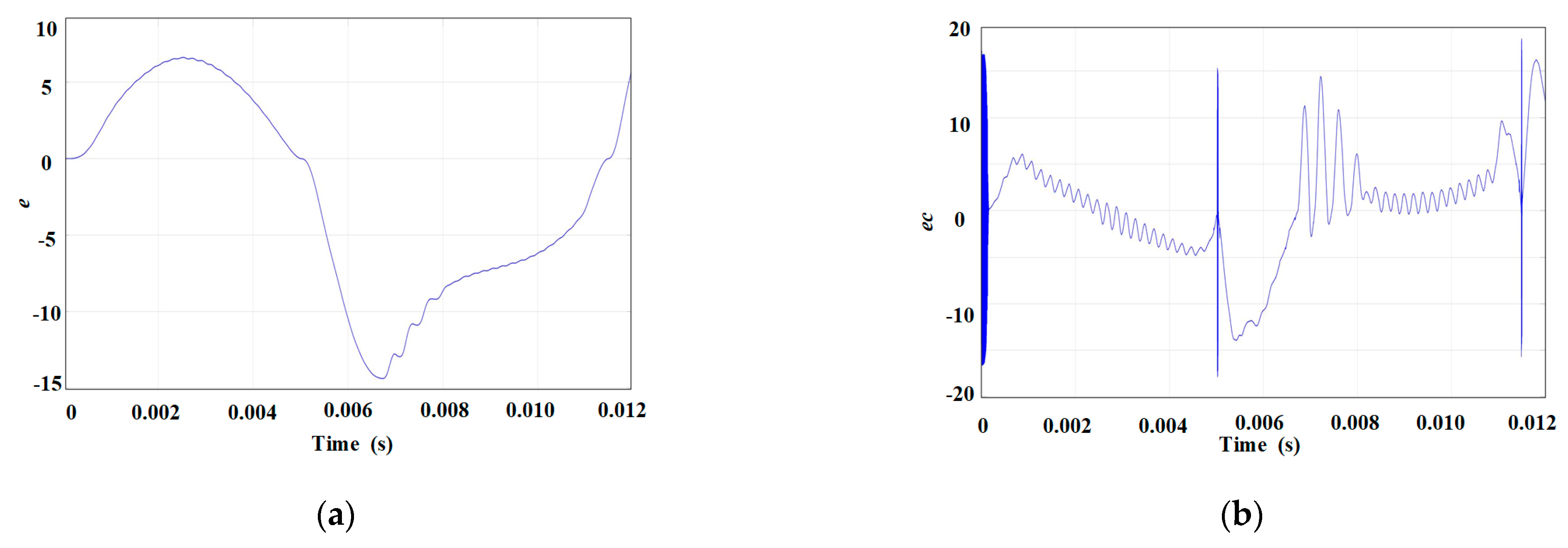
2.5. Fuzzy Model-Free Adaptive Control

Although adding a model-free adaptive component to the super-spiral observer enables it to adapt and compensate for estimation errors, it only adjusts the error through a single pseudo-bias. The fuzzy model-free adaptive control, on the other hand, adjusts the pseudo-bias using fuzzy adjustment parameters, which represents a further exploration to reduce the error.
Compared to the traditional model-free adaptive control, the fuzzy model-free adaptive control algorithm can dynamically update MFAC parameters online in real time, compensating for the error of the conventional super-spiral observer by dynamically updating MFAC parameters and ultimately improving estimation accuracy. The fuzzy model-free adaptive control structure is illustrated in Figure 4.
As shown in Figure 4, the fuzzy controller has two inputs and four outputs. The inputs are the error e and the rate of change of the error ec. The outputs are the variations in the step size factor Δρ, the variations in the weight factor Δλ, the variations in the pseudo-partial derivative weight factor Δμ, and the variations in the pseudo-partial derivative step size factor Δη.
The domain of e is [−2000, 2000], et is [−2, 2], Δρ is [0, 0.1], Δλ is [0, 0.2], Δη is [0, 0.2], and Δμ is [−150, 0]. The fuzzy subsets are [NB, NM, NS, ZO, PS, PM, PB], representing negative large, negative medium, negative small, zero, positive small, positive medium, and positive large, respectively. The membership functions are triangular. Through fuzzy inference and validation, the self-tuning rule tables, as shown in Table 1, Table 2 and Table 3, are obtained.
After referring to the relevant literature on MFAC and fuzzy control marriage, combined with the actual input and output parameters of the superhelix observer, the rules are as follows: Because the input signal of the superhelix observer is a sinusoidal signal with fluctuation, the amplitude of ec will increase significantly, and e will fluctuate near the equilibrium. This presents a challenge in designing fuzzy rules. When e and ec are too large, indicating a deviation from the equilibrium position, η should rise and μ should fall, improving the size of PPD, and increasing rapidity; when e and ec are both too small, it means that they are very close to the equilibrium position, η should fall, μ should rise, and the size of PPD should be reduced to avoid instability. The rules for Δρ and Δη are the same, except for Δλ, where the fuzzy rule for Δλ distinguishes between positive and negative, whereas the fuzzy rule for Δμ does not. Finally, through fuzzy reasoning and verification, the self-tuning rule table is obtained, as shown in Table 1, Table 2 and Table 3.
Due to the complex changes in ec, the changes in parameters (Δρ, Δη, Δλ, Δμ) are complicated. Their parameter-tuning rules are as follows: When e and ec increase, increase Δη and decrease Δμ to speed up the pseudo-bias change rate so that the system can quickly compensate for the error; improve system stability by increasing Δλ and reduce speed by decreasing Δρ to make the controller output as smooth as possible (and vice versa).
According to the above setting rules, the specific parameter adjustments of e and ec during a cycle of current error change, which spans from 0 to 0.011 s, are explained in detail. The changes of e and ec are shown in Figure 5.
The purpose of the fuzzy rule table is to make the error, e, closer to 0, as much as possible, by adjusting the parameters and counteracting the error in the reverse direction. The change in e is relatively slow, while the shift in ec is large. The adjustment process is divided into two stages according to the change in ec:
Stage 1: Within 0 to 0.0002 s, e is in a relatively stable state, and ec is in a precarious state for a short time, which is highly unfavorable to the motor estimation, so the impact on the estimation of the back electromotive force should be minimized. It is necessary to increase the variation of the pseudo-partial derivative significantly; that is, Δη is the largest and Δμ is the smallest. The output result needs to be compensated quickly while maintaining stability, so Δρ and Δλ are adjusted to be relatively large. The instantaneous adjustment method at 0.005 s and 0.011 s is equivalent to this state.
Stage two: Within 0.0002 s to 0.005 s, e increases first and then decreases, ec gradually becomes smaller, and the change slows down; at this time, it is necessary to reduce the pseudo-partial derivative so that the output change slows down, that is, Δη is larger and Δμ is smaller. At this time, the output compensation also needs to slow down; that is, Δρ first decreases and then increases, and Δλ gradually decreases. At the same time, adjusting the process by 0.005 s to 0.011 s is a significant improvement.

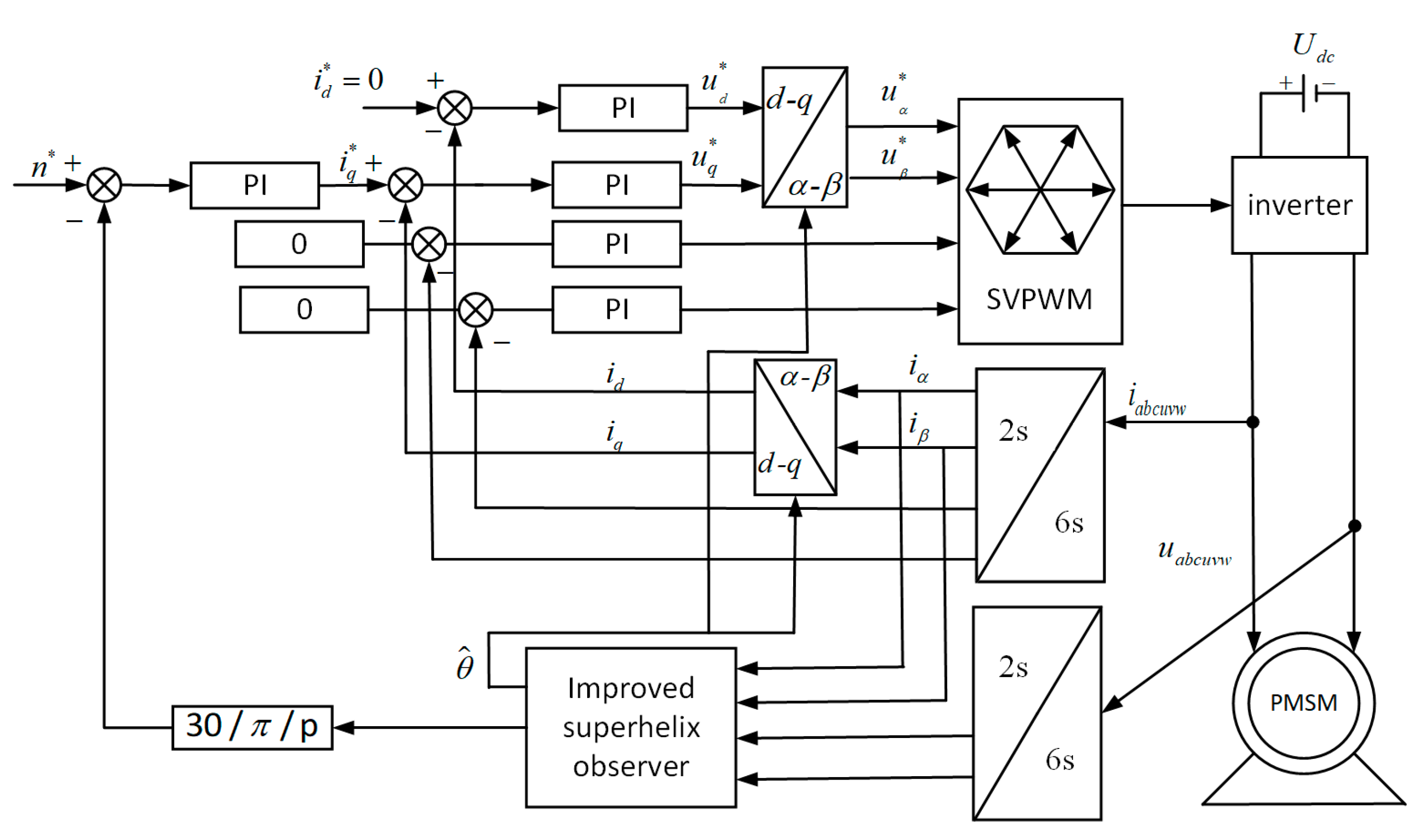
2.6. Design of an Improved Super-Twisting Observer

The improved super-twisting sliding-mode observer is as follows:
d i ^ α d t = R L i ^ α + 1 L u α 1 L e ^ m α ( k ) 1 L k 1 i α ˜ 1 / 2 sign ( i α ˜ ) 1 L k 2 sign ( i α ˜ ) d t d i ^ β d t = R L i ^ β + 1 L u β 1 L e ^ m β ( k ) 1 L k 1 i β ˜ 1 / 2 sign ( i β ˜ ) 1 L k 2 sign ( i β ˜ ) d t
By combining Equation (5), the improved no-model adaptive component of the back electromotive force em(k) can be expressed as follows:
ϕ ^ c ( k ) = ϕ ^ c ( k 1 ) + η + Δ η μ + Δ μ + Δ e m ( k 1 ) 2 Δ e m ( k 1 ) [ Δ Q ( k ) ϕ ^ c ( k 1 ) Δ e m ( k 1 ) ]
e m ( k ) = e m ( k 1 ) + ρ + Δ ρ λ + Δ λ + | ϕ ^ c ( k ) | 2 ϕ ^ c ( k ) [ Q * ( k + 1 ) Q ( k ) ]
If sign(φc(k)) ≠ sign(φc(1)) or |φc(k))| ≤ ε, then φc(k) = φc(1).
When the system reaches the sliding-mode surface, the estimated back electromotive force is expressed as follows:
e ^ α = e ^ m α ( k ) + 1 L k 1 i α ˜ 1 / 2 sign ( i α ˜ ) + 1 L k 2 sign ( i α ˜ ) d t e ^ β = e ^ m β ( k ) + 1 L k 1 i β ˜ 1 / 2 sign ( i β ˜ ) + 1 L k 2 sign ( i β ˜ ) d t
Because model-free adaptive control depends on the real-time update of the pseudo-partial derivative, the calculation time of model-free adaptive control is closely related to the sampling period, and the sampling period is taken as one calculation time. Traditional model-free adaptive control requires four operations in one cycle. The specific performance is as follows: 1. Calculate and improve the input signal Q*(k + 1) and Q(k). 2. Calculate the pseudo-partial derivative by Formula (2). 3. Calculate the initial input by Formula (1). 4. Obtain the estimated back electromotive force by improving the pseudo-bias reset algorithm.
Fuzzy model-free adaptive requires six operations in one cycle, which are shown as follows: 1. Calculate the improved input signals Q*(k + 1) and Q(k). 2. Calculate e and ec. 3. Calculate Δρ, Δλ, Δμ, Δη by fuzzy rules. 4. Calculate the pseudo-partial derivative by Formula (2). 5. Calculate the initial input by Formula (1). 6. Obtain the estimated back electromotive force by improving the pseudo-bias reset algorithm.
The control parameters k1 and k2 of the traditional superhelix observer are fixed, making it challenging to make corresponding adjustments to the complex current input signal. However, the improved superhelix observer, with the addition of model-less adaptive components, adjusts the output back electromotive force online through PPD to compensate for this defect, achieving even better control effects. μ, λ, ρ, and η of MFAC utilize fuzzy control to achieve greater flexibility, providing double assurance for optimal control results. This is also a strength of the approach used in this article.
Reference [30] shows that when the ratio of η/μ to ρ/λ is small, good stability can be obtained, but rapidity will be poor. Therefore, the selection of initial parameters is as follows: the η/μ ratio should be as small as possible to ensure slow fluctuations in pseudo-bias and enhance stability, and the ρ/λ ratio should be slightly larger to improve the rapidity of the output result.

3. Results and Discussion

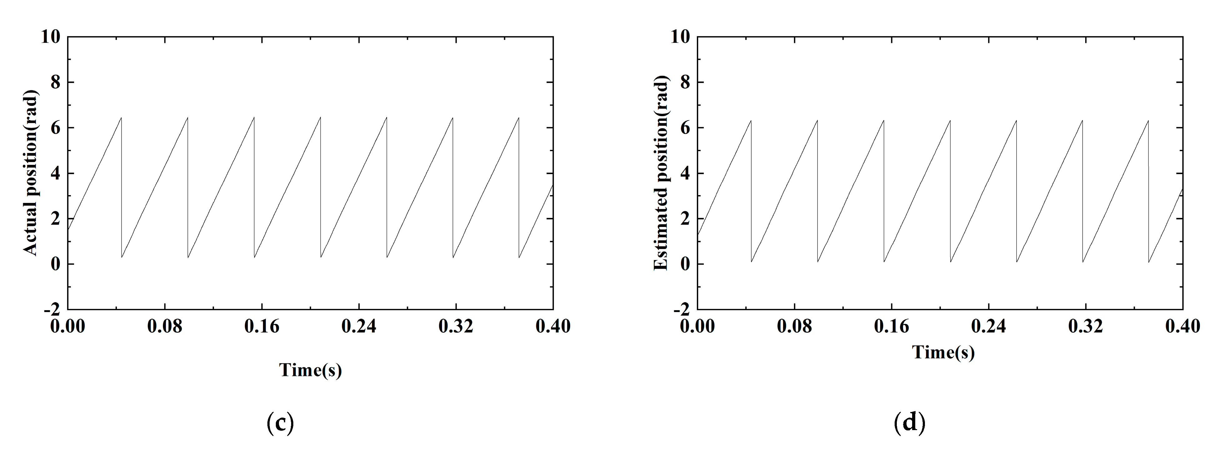
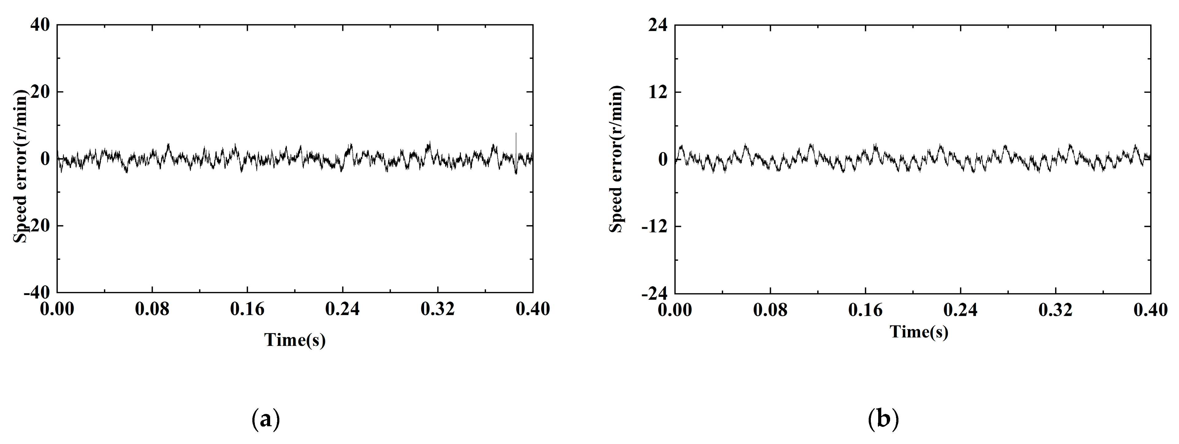
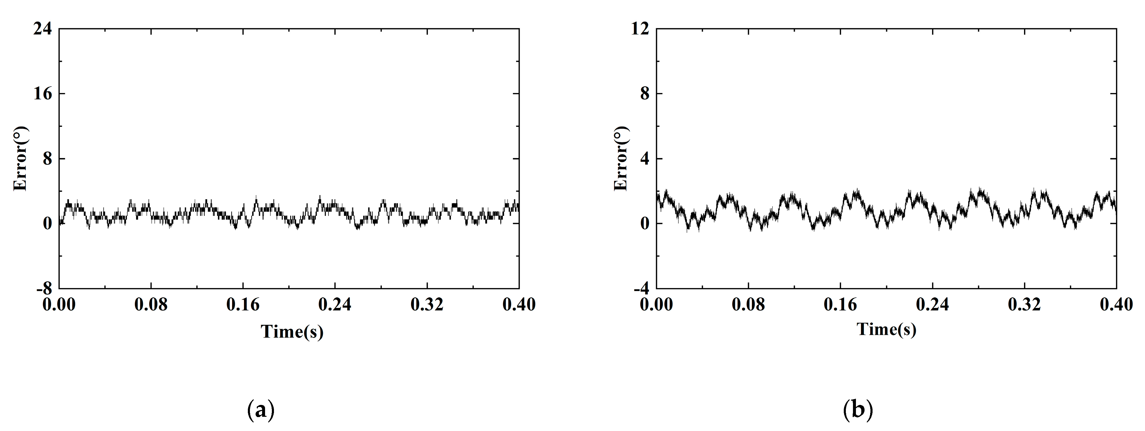
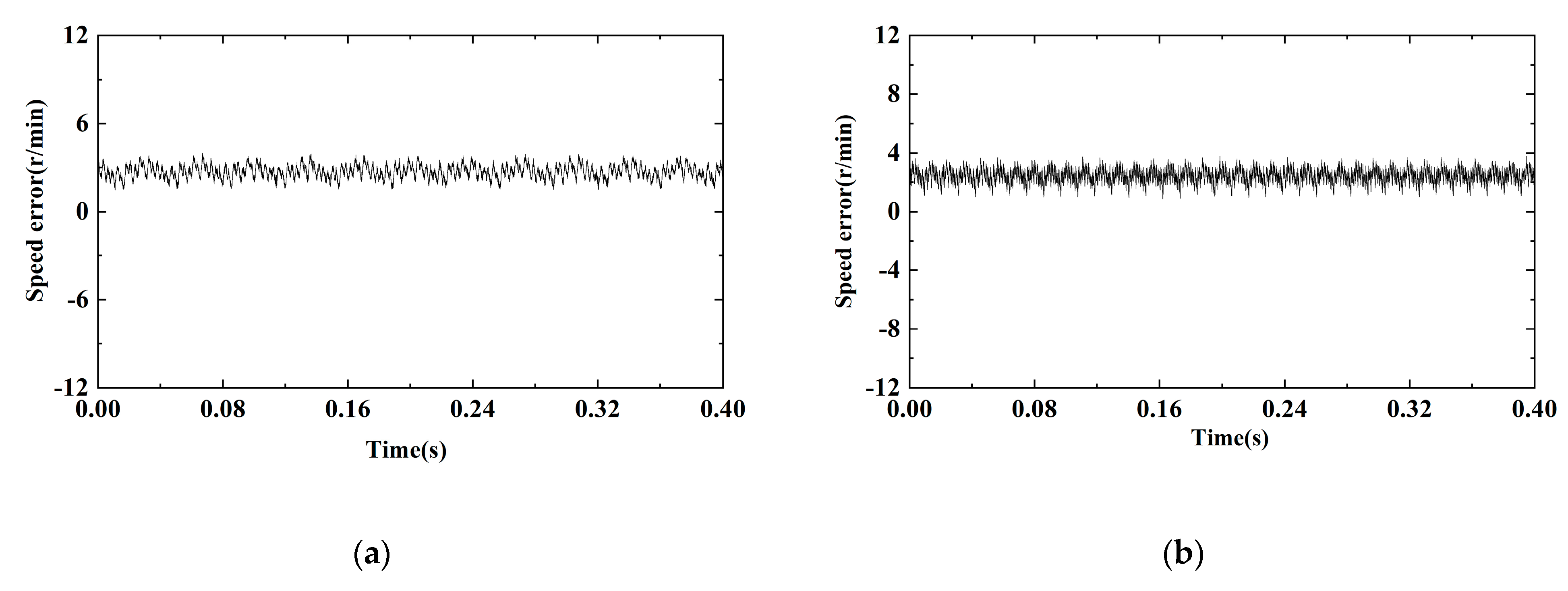
3.1. Simulation Verification

To verify that the position and angle observation accuracy of the fuzzy model-free adaptive control (FMFAC) superhelix observer is higher than that of the model-free adaptive control superhelix observer, At the same time, compared with traditional Super-Twisting Algorithm sliding mode observers (STA-SMO). This paper uses MATLAB/Simulink R2024b to conduct simulation experiments. The ode3 algorithm with a fixed step size is selected; the simulation step size is 2 × 10⁻⁶ s, and the simulation duration is 0.25 s. Set the initial speed to 500 r/min, increase the speed to 1000 r/min at 0.1, and increase the load at 0.2 s, where TL = 3 N·m.
The control method for a permanent magnet synchronous motor employs a three-phase PWM decoupling vector control. The moment of inertia of the simulated motor model is J = 0.015 kg·m2; the damping coefficient is B = 0; the pole number is Pn = 3; the Dc side voltage is Udc = 311 V, the PWM switching frequency is fpwm = 10 kHz, the target speed is set to 1000 r/min, and the MFAC parameters are η = 0.01, μ = 100, ρ = 0.8, λ = 0.8, a = 0.1, ε = 1 × 10⁻⁵, φc(k) = [1,1]T.
Figure 6 shows the change in current error and error change law, and Figure 7 shows the change of model-free adaptive parameters over time.
As shown in Figure 6a, the input error e changes relatively smoothly, indicating low control difficulty. However, the change rate of the input error ec in Figure 6b exhibits a wide variation range, which increases the difficulty of control. Such high-amplitude mutations drive the sudden changes in parameter values, so the parameter changes in Figure 7 may look chaotic, but they meet the two stages described in Figure 5, in Section 2.5; that is, the parameters can be adjusted in real time according to rapidly changing conditions to enhance control accuracy. This is why fuzzy model-free adaptive control is chosen.
From Figure 8, it can be seen that within 0 s to 0.1 s, given a speed of 500 r/min, the steady-state error of the MFAC speed after reaching the speed is within ±2 r/min, with a mean absolute error (MAE) = 1.339 and mean square error MSE = 3.571. The speed error is significant. The steady-state error of FMFAC adjusted by online parameters is within ±0.2 r/min or even smaller, MAE = 0.516, MSE = 1.547, and the estimation accuracy is significantly improved. Within 0.1 s to 0.2 s, given a speed of 1000 r/min, the steady-state error of MFAC is slightly reduced but remains within ±2 r/min, MAE = 1.089, MSE = 2.387, while the steady-state error of FMFAC can be maintained within 0 r/min to −1 r/min, MAE = 0.891, MSE = 1.619. Performance has also improved. In 0.2 s to 0.25 s, a specific load TL = 3 N·m is increased, and the steady-state error of rotational speed is also within ±2 r/min, MAE = 0.976, MSE = 1.484 The steady-state error of FMFAC can be maintained within 0 r/min to −1 r/min, with MAE = 0.603, MSE = 0.556. In general, it can be observed that in terms of speed error—both steady-state and dynamic conditions—the smaller MAE and MSE values for FMFAC indicate higher control accuracy compared to MFAC.
The MFAC and FMFAC position estimation errors are shown in Figure 9 for a given rotational speed of 500 r/min within 0 to 0.1 s. When the motor reaches a steady state, the rotor position error of MFAC is about 0.015 rad, where MAE = 0.022, MSE = 0.045, while the rotor position error of FMFAC is about 0.0125 rad after stability, and the steady-state error varies less, where MAE = 0.017, MSE = 0.035. Within 0.1 s to 0.2 s, the given speed is 1000 r/min; after the motor reaches a steady state, the MFAC rotor position error is about 0.03 rad, where MAE = 0.044 and MSE = 0.089. The FMFAC rotor position error is about 0.025 rad, with MAE = 0.035 and MSE = 0.071. The load of TL = 3 N·m is applied in 0.2 to 0.25 s. It can be seen from the figure that the steady-state errors of MFAC and FMFAC remain relatively unchanged. In MFAC, MAE = 0.048 and MSE = 0.116; in FMFAC, MAE = 0.039 and MSE = 0.094. In summary, compared to MFAC in rotor position estimation, FMFAC control accuracy is also improved.
As can be seen from Figure 10a, the rated speed is 500 r/min between 0 and 0.1 s. The speed estimation error of traditional super-helical observers ranges from approximately −3 r/min to 4 r/min. MAE = 1.993 and MSE = 7.213. Between 0.1 s and 0.2 s, the rated speed is 1000 r/min, and the error is roughly between −2 r/min and 6 r/min. MAE = 2.607 and MSE = 11.040. Between 0.2 and 0.25 s, a load of TL = 3 N·m is applied. The range of error is small, MAE = 2.347, and MSE = 7.828. Similarly, in Figure 10b, between 0 and 0.1 s, the position error is approximately 0.02 rad, with MAE = 0.036 and MSE = 0.105. Between 0.1 and 0.2 s, the position error is around 0.04 rad, MAE = 0.057, and MSE = 0.109. Between 0.2 and 0.25 s, MAE = 0.063 and MSE = 0.148.
Compared with Figure 8, Figure 9 and Figure 10, it can be seen that although the traditional super-spiral observer exhibits relatively good control performance, the estimation accuracy can be further improved without the addition of model adaptive control, resulting in significant reductions in MAE and MSE.
Although the control effect of FMFAC is better than that of MFAC, the introduction of fuzzy control undoubtedly increases the system’s complexity and raises higher requirements for its computing power.

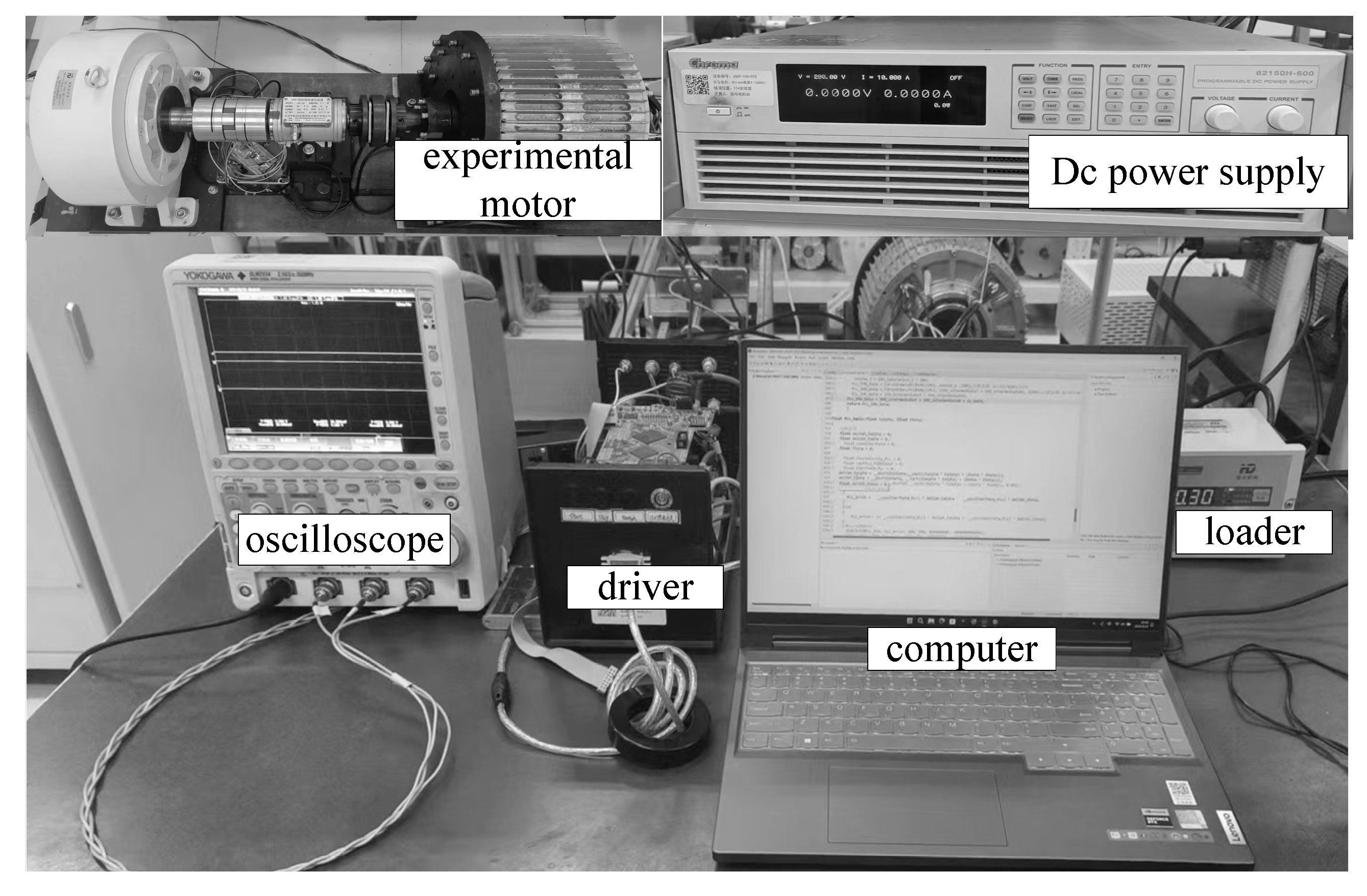
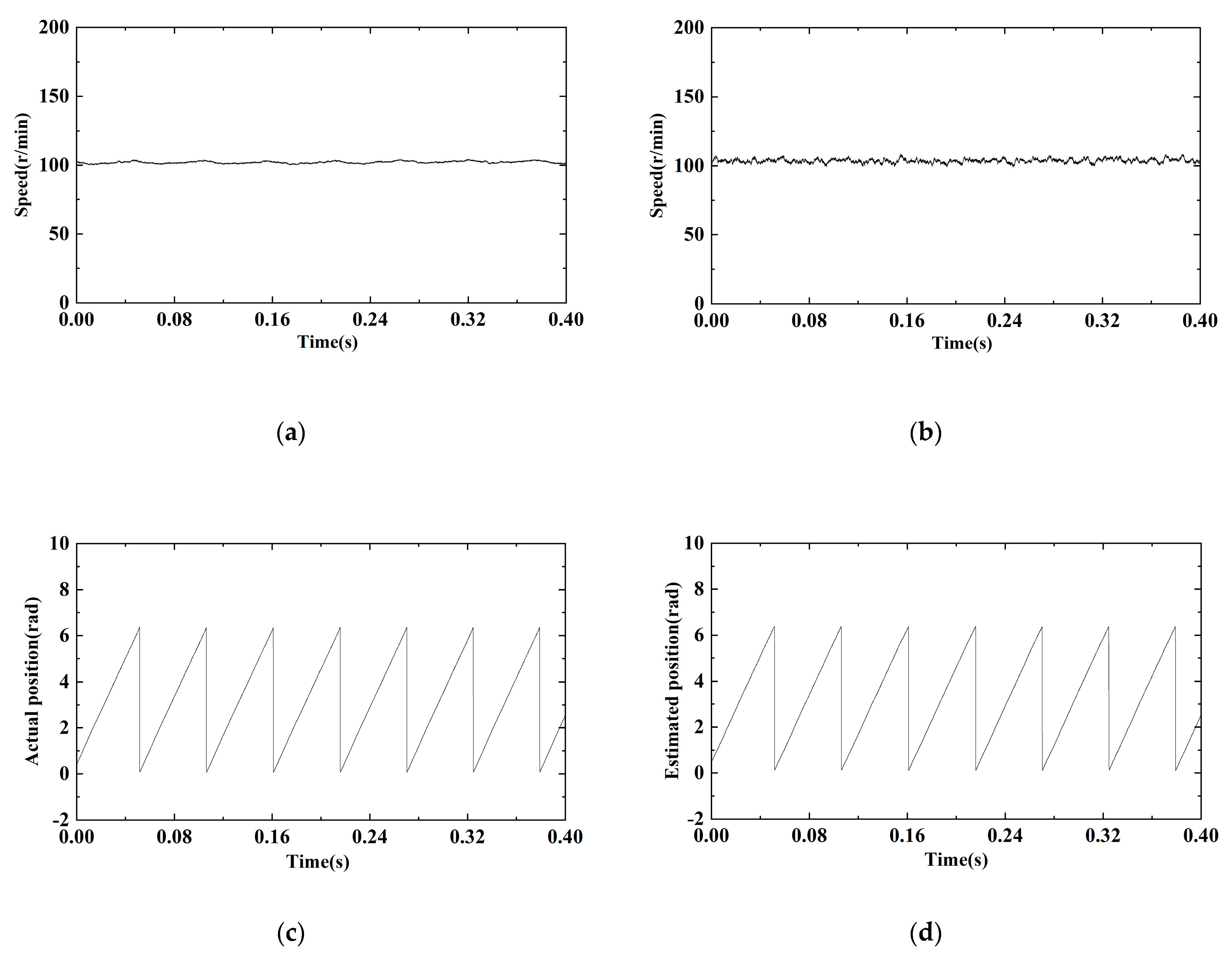
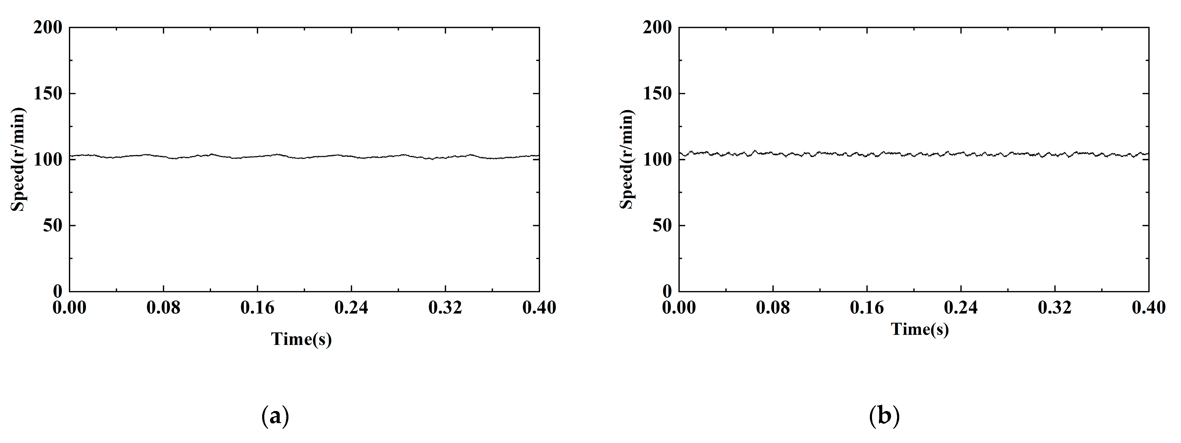
3.2. Experimental Verification

To verify the feasibility of the improved super-twisting sensorless control algorithm, an experimental platform was established. The system structure diagram is shown in Figure 11, and the parameters of the permanent magnet synchronous motor are listed in Table 4. The experimental platform, as shown in Figure 12, was built for experimental verification. The sampling period is 10−4 s.
During system startup under load conditions, the load torque is TL = 40 N·m. The given rotor speed is 100 r/min. Figure 13 shows the speed and position data for the STA-SMO algorithm, while Figure 14 presents the speed and position data for the MFAC-SMO algorithm.
Figure 13a and Figure 14a show that the actual speeds of the STA-SMO and MFA-SMO methods do not change significantly; the key error originates from the different methods used in Figure 13b and Figure 14b. The rotor estimation method in Figure 13b adopts the traditional superhelix observer, with fixed gains k1 and k2 that remain unchanged. This results in relatively high jitter in the estimated speed. In contrast, the jitter in Figure 14b is smaller than that in Figure 13b because the model-free adaptive component is added to compensate for the fixed gain. From Figure 13c,d and Figure 14c,d, it can be seen that the actual position signal of the rotor and the estimated position signal make it difficult to see the difference between the two methods because the amplitude of change is too fast and the error is too small. Therefore, the rotor position error in Figure 15 was selected to make a more in-depth comparison.
As can be seen from Figure 15, when the given speed of 100 r/min is stabilized, the STA-SMO used in Figure 15a has a larger speed estimation error, with a maximum estimated error of 6.2 r/min, MAE = 1.171, and MSE = 2.185. The estimated error of the MFAC-SMO used in Figure 15b is significantly smaller, with the maximum estimated error being 2.7 r /min, with MAE = 0.772 and MSE = 0.997, indicating better performance. The same applies to rotor position information. In Figure 16a, the maximum rotor position estimation error for STA-SMO is 3.36°, with MAE = 1.168, and MSE = 1.926. In Figure 16b, the maximum rotor position estimation error for MFAC-SMO is 2.27°, with MAE = 0.837 and MSE = 0.986, with MSE being significantly reduced. It can be seen that in addressing the problem of fixed gains in traditional super-helical observers, adding model-free adaptive components can effectively reduce estimation error and improve estimation accuracy.
Figure 17 shows the error change of the motor when the load is changed to TL = 60 N·m. The STA-SMO speed error is shown in Figure 17a, with MAE = 2.839 and MSE = 7.590; the MFA-SMO speed error is shown in Figure 17b, with MAE = 2.417 and MSE = 6.064; the STA-SMO position error is shown in Figure 17c, with MAE = 1.018 and MSE = 1.474. The position error of MFAC-SMO is shown in Figure 17d, with MAE = 0.739 and MSE = 1.026. It can be seen that under load variation, MFAC-SMO can still have better control performance.
Although the control effect of MFAC-SMO is better than that of STA-SMO, the introduction of the no-model adaptive component also increases the number of adjustment parameters, making the control system more complex.

4. Conclusions

The main contributions of this paper are as follows: Fuzzy model-free adaptive control is used to compensate for the position error of the super-spiral observer. The introduction of model-free adaptive components expands the application of online adjustment parameters in the observer. The general rules for fuzzy rule tables and parameter adjustments are summarized, providing an essential theoretical and data reference for the popularization and application of fuzzy model-free adaptive control.
However, FMFAC also has some limitations, and it is more suitable for occasions where control accuracy is high and external interference is significant. At the same time, it imposes higher requirements on the system’s computing power.
The specific reasons are as follows: Due to the discreteness of MFAC, a delay module needs to be added. However, in the double closed-loop system, the introduction of a delay module will have a significant impact on the system speed. Whether it is the early start speed of the motor or the anti-interference ability, MFAC makes it challenging to meet the requirements. MFAC can only be used in a single closed-loop system, such as an observer. The false reset of the false deviation also complicates the method. Fuzzy model-free adaptive control can only be adjusted effectively within the fine-tuning range. The initial parameters of model-free adaptive control systems are different. Therefore, the popularity of fuzzy model-free adaptive methods is often gained through experience or parameter adjustment.
Given these limitations, the future research directions are mainly as follows:
  • Explore the principles of parameter adjustment to simplify the adjustment process.
  • Utilize model-free adaptive predictive control to enhance the control effect and effectively address the inherent fuzziness of model-free adaptive predictive control systems.
  • Further reduce the amplitude of parameter variation in model-free adaptive parameters for fuzzy systems to strengthen the control effect.

Author Contributions

D.Z.: methodology, supervision, project administration, conceptualization; B.Z.: software, writing—reviewing, editing writing—original draft preparation investigation, formal analysis; T.T.: validation, data curation. All authors have read and agreed to the published version of the manuscript.

Funding

This research was funded by the National Natural Science Foundation of China, grant no. 52107047.

Data Availability Statement

Data are contained within the article.

Acknowledgments

The authors would like to thank Cao Jun-hui for his help with the speed and position analyses in Figure 6 (STA-SMO) and Figure 7 (MFA-SMO), the speed errors of the two methods in Figure 8, and the position errors of the two methods in Figure 9.

Conflicts of Interest

The authors declare no conflicts of interest.

References

  1. Gaolin, W.; Maria, V.; Jorge, S. Position Sensorless Permanent Magnet Synchronous Machine Drives—A Review. IEEE Trans. Ind. Electron. 2020, 67, 5830–5842. [Google Scholar]
  2. Ding, H.; Zou, X.; Li, J. Sensorless Control Strategy of Permanent Magnet Synchronous Motor Based on Fuzzy Sliding Mode Observer. IEEE Access 2022, 10, 36743–36752. [Google Scholar] [CrossRef]
  3. Yuan, X.; Yang, Z.B.; Xun, L.J. Position Sensorless control strategy of permanent magnet synchronous motor based on improved sliding mode observer. Small Spec. Electr. Mach. 2022, 50, 47–52. [Google Scholar]
  4. Ton, N.; Trung, T.; Hoang, T. An Adaptive Backstepping Sliding-Mode Control for Improving Position Tracking of a Permanent-Magnet Synchronous Motor with a Nonlinear Disturbance Observer. IEEE Access 2023, 11, 19173–19185. [Google Scholar]
  5. Sun, Q.G.; Zhu, X.L.; Nin, F. Position Sensorless Control of Permanent Magnet Synchronous Motor Based on Improved Integral Sliding Mode Observer. In Proceedings of the 2024 IEEE PES 16th Asia-Pacific Power and Energy Engineering Conference (APPEEC), Nanjing, China, 25–27 October 2024; Volume 48, pp. 3269–3278. [Google Scholar]
  6. Mei, S.G.; Lu, W.Z.; Fan, Q.G. Position Sensorless Control Strategy for Permanent Magnet Synchronous Motors Based on Sliding Mode Observer Error Compensation. Trans. China Electrotech. Soc. 2023, 38, 398–408. [Google Scholar]
  7. Wang, J.; Zhou, L.; Su, M.X. Sensorless control of adaptive super spiral sliding mode observer based on fuzzy control. J. Electr. Eng. 2023, 18, 32–42. [Google Scholar]
  8. Kang, E.J.; Chen, J. Improved sliding mode sensorless control of permanent magnet synchronous motor. Electr. Mach. Control 2022, 10, 88–97. [Google Scholar]
  9. Shi, Q.G.; Zhu, J.J.; Han, Y. Load torque identification of permanent magnet synchronous motor based on adaptive sliding mode observer. Trans. China Electrotech. Soc. 2025, 1–15. [Google Scholar]
  10. Zhang, Y.H.; Cai, Q.L.; Cui, W.T. Sensorless Control of Permanent Magnet Synchronous Motor Using a New-type Sliding Mode Observer. Electr. Eng. 2024, 21, 94–97. [Google Scholar]
  11. Xu, W.; Jia, H.P. Sensorless Control of Permanent Magnet Synchronous Motor Based on Improved Sliding-Mode Observer. Electron. Packag. 2024, 24, 123–128. [Google Scholar]
  12. Wang, L.; Wang, Y.A.; Wu, J.K. Research on Control of Improved Super-Spiral Sliding Mode Observer for Permanent Magnet Synchronous Motor. Electrotech. Electr. 2024, 8, 15–20+25. [Google Scholar]
  13. Yu, H.; Zhou, S.G.; Ma, F.H. Sensorless Control of PMSM Based on Fuzzy Full-order Sliding Mode Observer. Electr. Drive 2024, 54, 3–10. [Google Scholar]
  14. Wang, X.L.; Xu, Z.C. Research on PMSM Control Based on Improved Sliding Mode Observer. Ind. Control Comput. 2024, 37, 26–28. [Google Scholar]
  15. Abdülhamit, N.; Nihat, İ. Sensorless Vector Control for Induction Motor Drive at Very Low and Zero Speeds Based on an Adaptive-Gain Super-Twisting Sliding Mode Observer. IEEE J. Emerg. Sel. Top. Power Electron. 2023, 11, 4332–4339. [Google Scholar]
  16. Sun, X.L.; Zhou, L.; Tian, Y.A. Sensorless Control Based on Fuzzy Variable Coefficient Super Twisting Sliding Mode Observer. J. Power Supply 2025, 1–14. [Google Scholar]
  17. Kanat, S.; Ton, D. Design and Analysis of a Generalized High-Order Disturbance Observer for PMSMs With a Fuzy-PI Speed Controller. IEEE Access 2022, 10, 42252–42260. [Google Scholar]
  18. Zheng, R.; Zhang, J.X.; Dong, X.S. Permanent magnet synchronous motor BP neural network-intelligent PID sliding mode observation vector control algorithm. J. Detect. Control 2024, 46, 124–131. [Google Scholar]
  19. Wu, X.H.; Liu, Y.T.; Chen, H.L. Recurrent Neural Network-Based Model Predictive Control for Speed Regulation in Permanent Magnet Synchronous Motors with an Extended Sliding Mode Load Torque Observer. In Proceedings of the 2024 IEEE 7th International Electrical and Energy Conference (CIEEC), Harbin, China, 10–12 May 2024; pp. 3689–3694. [Google Scholar]
  20. Shilpa, Y.; Anurodh, K.; Amit, V. Torque Estimation of Permanent Magnet Synchronous Motor (PMSM) Using 1D Convolutional Neural Network. In Proceedings of the 2022 IEEE 6th Conference on Information and Communication Technology (CICT), Gwalior, India, 18–20 November 2022; pp. 1–5. [Google Scholar]
  21. Lin, X.P.; Xu, R.Q.; Yao, W.R. Observer-Based Prescribed Performance Speed Control for PMSMs: A Data-Driven RBF Neural Network Approach. IEEE Trans. Ind. Inform. 2024, 20, 7502–7512. [Google Scholar]
  22. Jiang, Y.; Gao, W.N.; Wu, Q. Reinforcement learning and cooperative H∞ output regulation of linear continuous-time multi-agent systems. Automatica 2023, 148, 110768. [Google Scholar]
  23. Shi, H.Y.; Gao, W.; Jiang, X.Y. Two-dimensional model-free Q-learning-based output feedback fault-tolerant control for batch processes. Comput. Chem. Eng. 2024, 184, 108583. [Google Scholar]
  24. Zhang, X.J.; Bujarbaruah, M.; Borrelli, F. Near-Optimal Rapid MPC Using Neural Networks: A Primal-Dual Policy Learning Framework. IEEE Trans. Control Syst. Technol. 2021, 29, 2102–2114. [Google Scholar]
  25. Farzanegan, B.; Moghadam, R.; Jagannathan, S. Optimal Adaptive Tracking Control of Partially Uncertain Nonlinear Discrete-Time Systems Using Lifelong Hybrid Learning. IEEE Trans. Neural Netw. Learn. Syst. 2024, 35, 17254–17265. [Google Scholar] [PubMed]
  26. Tesfazgi, S.; Sprandl, L.; Lederer, A. Stable Inverse Reinforcement Learning: Policies from Control Lyapunov Landscapes. IEEE Open J. Control Syst. 2024, 3, 358–374. [Google Scholar]
  27. Wang, S.D.; Dragicevic, T.; Gontijo, G.F.; Chaudhary, S.K. Machine Learning Emulation of Model Predictive Control for Modular Multilevel Converters. IEEE Trans. Ind. Electron. 2021, 68, 11628–11634. [Google Scholar]
  28. Grelewicz, P.; Khuat, T.T.; Czeczot, J. Application of Machine Learning to Performance Assessment for a Class of PID-Based Control Systems. IEEE Trans. Syst. Man Cybern. Syst. 2023, 53, 4226–4238. [Google Scholar] [CrossRef]
  29. Ho, M.C.; Lim, J.M.; Chong, C.Y. High-Dimensional Origin Destination Calibration Using Metamodel Assisted Simultaneous Perturbation Stochastic Approximation. IEEE Trans. Intell. Transp. Syst. 2023, 24, 3845–3854. [Google Scholar]
  30. Feng, Z.X.; Ren, Q.C.; Reng, Y.P. Optimizing the Parameters of MFAC Based on the Simplex Method. Control Eng. China 2016, 23, 405–410. [Google Scholar]
Figure 1. MFAC algorithm flow chart.
Energies 18 01877 g001
Figure 2. Traditional model-free adaptive parameters: (a) current error; (b) PPD reset symbol; (c) PPD; and (d) speed error.
Energies 18 01877 g002aEnergies 18 01877 g002b
Figure 3. Improved model-free adaptive parameters: (a) current error; (b) PPD reset symbol; (c) PPD; and (d) speed error.
Energies 18 01877 g003
Figure 4. Fuzzy model-free adaptive control structure.
Energies 18 01877 g004
Figure 5. Input error variation within the FMFAC part: (a) e varies with time; (b) ec varies with time.
Energies 18 01877 g005
Figure 6. FMEAC input error changes: (a) e varies with time; (b) ec varies with time.
Energies 18 01877 g006
Figure 7. The MFAC parameter changes: (a) η varies with time; (b) μ varies with time; (c) ρ varies with time; and (d) λ varies with time.
Energies 18 01877 g007
Figure 8. Speed errors of MAFC and FMAFC: (a) MAFC speed error; (b) FMAFC speed error.
Energies 18 01877 g008
Figure 9. Position errors of MAFC and FMAFC (a) MFAC position error; (b) FMFAC position error.
Energies 18 01877 g009
Figure 10. STA-SMO errors: (a) STA-SMO speed error; (b) STA-SMO position error.
Energies 18 01877 g010
Figure 11. Based on the MFAC-SMO control block diagram.
Energies 18 01877 g011
Figure 12. Permanent magnet synchronous motor experiment platform.
Energies 18 01877 g012
Figure 13. STA-SMO speed and position: (a) actual speed; (b) estimated speed; (c) actual position; and (d) estimated position.
Energies 18 01877 g013
Figure 14. MFAC-SMO speed and position: (a) actual speed; (b) estimated speed; (c) actual position; and (d) estimated position.
Energies 18 01877 g014aEnergies 18 01877 g014b
Figure 15. The speed errors of the two methods: (a) STA-SMO speed error and (b) MFAC-SMO speed error.
Energies 18 01877 g015
Figure 16. The position errors of the two methods: (a) STA-SMO position error and (b) MFAC-SMO position error.
Energies 18 01877 g016
Figure 17. Errors at load TL = 60 N·m: (a) STA-SMO speed error; (b) MFAC-SMO speed error; (c) STA-SMO position error; and (d) MFAC-SMO position error.
Energies 18 01877 g017aEnergies 18 01877 g017b
Table 1. Fuzzy rules Δρ and Δη.
eec
NBNMNSZOPSPMPB
NBPBPMPSZOPMPBPB
NMPMPSZONSPSPMPB
NSPSZONSNMZOPSPM
ZOZONSNMNBNMNSZO
PSPBPSZONMNSZOPS
PMPBPMPSNSZOPSPM
PBPBPBPMZOPSPMPB
Table 2. Fuzzy rules Δλ.
eec
NBNMNSZOPSPMPB
NBNBNMNMNSZOPSPM
NMNBNMNMNSZOPSPM
NSNBNMNSZOPSPMPM
ZONMNMNSZOPSPMPM
PSNMNMNSZOPMPMPB
PMNMNSZOPMPMPBPB
PBNMNSPSPMPMPBPB
Table 3. Fuzzy rules Δμ.
eec
NBNMNSZOPSPMPB
NBNBNMNSZONMNBNB
NMNMNSZOPSNSNMNB
NSNSZOPSPMZONSNM
ZOZOPSPMPBPMPSZO
PSNBNSZOPMPSZONS
PMNBNMNSPSZONSNM
PBNBNBNMZONSNMNB
Table 4. Parameters of the permanent magnet synchronous motor.
Parameter NameValue
Number of poles11
Stator resistance/Ω0.92
dq-axis inductance/mH15.21
Rotor flux linkage/Wb0.88
Disclaimer/Publisher’s Note: The statements, opinions and data contained in all publications are solely those of the individual author(s) and contributor(s) and not of MDPI and/or the editor(s). MDPI and/or the editor(s) disclaim responsibility for any injury to people or property resulting from any ideas, methods, instructions or products referred to in the content.

