A Modularity-Enhanced Echo State Network for Nonlinear Wind Energy Predicting

Abstract

With the rapid growth of wind power generation, accurate wind energy prediction has emerged as a critical challenge, particularly due to the highly nonlinear nature of wind speed data. This paper proposes a modularized Echo State Network (MESN) model to improve wind energy forecasting. To enhance generalization, the wind speed data is first decomposed into time series components, and Modes-cluster is employed to extract trend patterns and pre-train the ESN output layer. Furthermore, Turbines-cluster groups wind turbines based on their wind speed and energy characteristics, enabling turbines within the same category to share the ESN output matrix for prediction. An output integration module is then introduced to aggregate the predicted results, while the modular design ensures efficient task allocation across different modules. Comparative experiments with other neural network models demonstrate the effectiveness of the proposed approach, showing that the statistical RMSE of parameter error is reduced by an average factor of 2.08 compared to traditional neural network models.

1. Introduction

In recent years, the renewable energy industry has seen significant development and growth, with wind energy being the pivotal component of the renewable energy industry [1]. The total installed capacity of wind energy in 2023 was 117 GW, a 50% year-on-year increase from 2022. Meanwhile, Global Wind Energy Council (GWEC) forecasts an additional 1210 GW of global wind energy from 2024–2030 [2]. However, the inherent randomness and non-linearity of the wind variability can lead to volatility in wind power generation, posing challenges to grid stability [3]. Therefore, accurate wind speed prediction is essential for ensuring a reliable electricity supply and optimizing grid stability.

According to current research, wind speed prediction methods can be classified into physical prediction methods [4], traditional statistical methods [5], and machine learning and neural network methods [6,7]. Physical methods predict wind speed and direction by modeling atmospheric motion, but are computationally expensive due to shortcomings in boundary conditions and model complexity [8]. Unlike physical methods, traditional statistical methods do not account for the physical environmental factors surrounding the wind turbine. These methods include the autoregressive model (AR) [9], the autoregressive moving average model (ARMA) [10], the autoregressive integrated moving average model (ARIMA) [11], among others. However, extensive research has shown that traditional statistical methods are inadequate for nonlinear data due to their inherent stability assumptions, making them less suitable for forecasting nonlinear wind speed variations.

Machine learning methods and neural networks have garnered significant attention for their strong performance in nonlinear prediction. Notable models include Recurrent Neural Network (RNN) [12], Long Short-Term Memory (LSTM) [13], Gate Recurrent Unit (GRU) [14] and Echo State Networks (ESN) [15]. Neural networks are highly effective in handling noisy data and capturing complex non-linear relationships between inputs and outputs, making them particularly effective for forecasting wind speed [16]. However, neural networks also have limitations in wind speed prediction. Even small errors in the dataset can substantially affect their performance [17].

To address the sensitivity of neural networks, many researchers have investigated approaches such as integrating different neural networks [18] or introducing modularity [19,20]. The primary goal of modular neural networks is to decompose a neural network into multiple functional modules, thereby minimizing ambiguity in knowledge storage and improving both accuracy and robustness. Additionally, due to the independence of each module, modular networks offer greater flexibility—allowing modifications or replacements of specific components without requiring a complete network reconstruction when adapting to different datasets. Furthermore, modularization enables efficient task distribution, allowing neural networks to assign tasks based on specialized modules, ultimately enhancing model performance.

Modular neural networks can be categorized into sample-based [21], feature-based, and model-based architectures, each serving distinct applications in various models. Aljundi et al. integrated a sample-based modular neural network into a lifelong learning framework, utilizing Auto-Encoder reconstruction error to discover category hierarchies and faciliate information routing [22]. However, its knowledge module design lacks flexibility, and determining the category hierarchy remains challenging. Zhou et al. developed a deep clustering model by combining a representation learning module with a clustering module, forming a feature-based modular neural network [23]. Their method employs a multilevel, generative, iterative, and synchronized approach for deep clustering classification. However, it compromises feature extraction quality, which can significantly impact modular network performance when applied to datasets with weakly distinguishable features, ultimately reducing efficiency.

P. Kontschieder proposed a model-based modular neural network that integrates a microscopic decision tree model with a deep neural network for representation learning. This approach reduces the uncertainty of routing decisions at split nodes, optimizesmodel performance, and ultimately results in a physically modular neural network [24]. A key advantage of model-based modular neural networks is their adaptability, as they dynamically adjust to data by leveraging modular divisions, thus enhancing both flexibility and interpretability. However, the lack of direct constraints on features may lead to ambiguities in module characterization within the model. Modular neural networks have also been applied in the prediction of wind energy, where turbines within the same wind farm share similar geographic and climatic conditions. Given these similarities in local characteristics, the combination of model-based and feature-based modular neural networks can improve wind energy forecasting by leveraging both structured modular adaptation and relevant local characteristic references across different tasks.

However, modular neural networks also have intrinsic limitations, with one significant challenge being the adaptation between the network architecture and the assigned task. Li et al. developed an adaptive modular neural network based on feature clustering to model a nonlinear system and compared its performance with three other modular neural networks, revealing significant discrepancies in results [25]. This highlights that a poor match between the network structure and the task can lead to reduced model effectiveness, even when tested on similar datasets.

Despite these challenges, modular neural networks continue to offer unique advantages depending on the application domain, design strategy, and dataset characteristics. In wind energy prediction, for instance, Shang et al. introduced a network model-building module to mitigate the computational complexity of CNNs, which typically require multiple hidden layers for effective predictions [26]. Chen et al. incorporated the NFLBlock module into a wind power prediction model to normalize input data and employed a stacked multilayer perceptron to capture inter-temporal and inter-dimensional dependencies. This strategy reduced the interference of dynamic features, thereby enhancing prediction accuracy while lowering computational costs [27]. Furthermore, Huan et al. leveraged a direct embedding module with a cross-attention mechanism to overcome the limitations of traditional Transformers in capturing temporal dependencies, ultimately improving wind speed prediction performance [28].

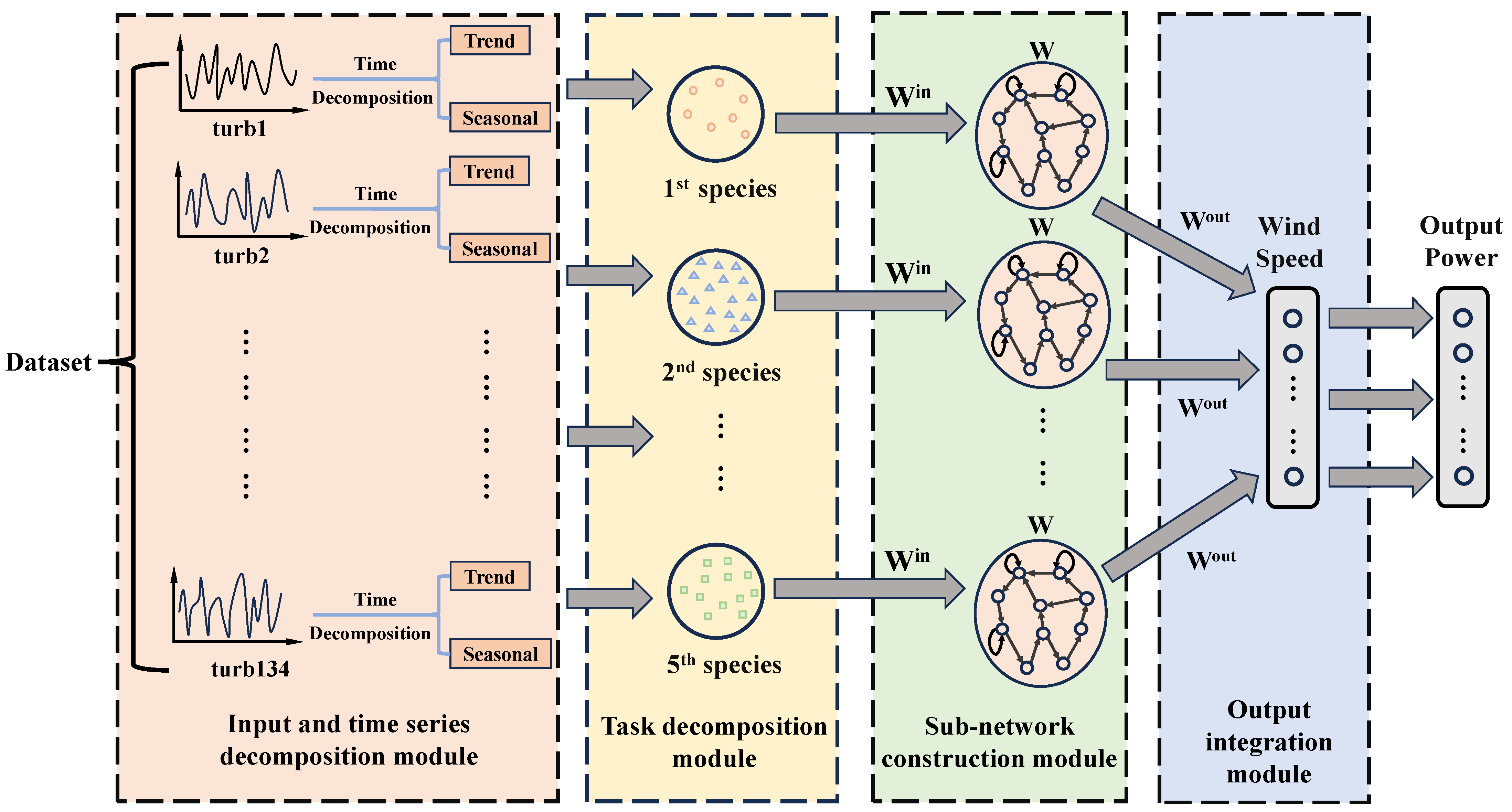
Building on the analysis of historical methods and modularization in wind energy prediction, this paper proposes a Modular Echo State Network (MESN) model to improve prediction accuracy. The approach begins with segmenting wind turbine data, applying pre-processing to eliminate outliers, and performing a time series decomposition into trend, seasonal, and residual components. The trend and seasonal terms are predicted separately using ESN and then combined. To optimize learning, Modes cluster is used to group trend patterns on a daily basis for pre-training in the ESN output layer. Additionally, turbine clusters group wind turbines with similar wind speed and energy characteristics, allowing them to share the same ESN output matrix. An output aggregation algorithm then integrates predictions across different turbine groups, while modularization ensures efficient task allocation. Finally, wind energy forecasts are obtained by leveraging the conversion relationship between wind speed and energy.

The main contributions of the model are as follows:

• A neural network wind energy prediction model that integrates modularization is proposed to make predictions based on different data features. The problem of task allocation is solved.
• In the Output integration module, a novel integration algorithm is proposed to integrate the data assigned to different tasks.
• The wind speed prediction model proposed in this paper is applied to wind energy prediction. In addition, in-depth analysis and experiments are conducted, and the results show that the method proposed in this paper enhances the prediction accuracy.

This paper is organized as follows: the second part describes the MESN modeling process and the theoretical derivation of the method. The third part provides a detailed description of the experimental process and compares it with other models to demonstrates the efficacy of the prediction method proposed in this paper. The fourth part summarizes the conclusions and outlook of this paper.

2. Construction of MESN

For the uniqueness of the selected dataset in this paper, we improved the ESN model and proposed the MESN model to forecast the wind turbine data. The basic framework of MESN is shown in Figure 1.

2.1. Input and Time Series Decomposition Module

The first module is the input and time series decomposition module, which decomposes the wind speed dataset into trend, seasonal, and residual components after data pre-processing. The time series decomposition method used in this paper follows a multiplicative decomposition approach, where the wind speed data at time t is represented as a multivariate time series $Y_t\in {\mathbb{R}}^{N\times d}$, where N is the number of wind turbines and d is the number of time steps. Each row of $Y_t$ corresponds to the wind speed observations from a specific turbine, denoted as

$$y_n=[y_{n_1},y_{n_2},\dots ,y_{n_d}]\in {\mathbb{R}}^d,n=1,2,\dots ,N.$$

The decomposition follows the relation:

$$Y_t=T_t\times S_t\times R_t,$$

(1)

where $T_t$ represents the trend component, obtained using a moving average method to mitigate short-term fluctuations while preserving long-term patterns. The seasonal component $S_t$ is computed by normalizing the original wind speed data with the trend component, expressed as:

$$S_t={\displaystyle \frac{Y_t}{T_t\times R_t}}$$

(2)

The residual component $R_t$ captures variations unexplained by the trend and seasonal components and is given by:

$$R_t={\displaystyle \frac{Y_t}{T_t\times S_t}}.$$

(3)

This decomposition provides a structured representation of wind speed dynamics, enabling more robust predictive modeling.

2.2. Task Decomposition Module

The second module is the pattern clustering module for trends, where clustering is performed on two different objects.

2.2.1. Modes-Cluster

Clustering of K-means is applied first to wind speed patterns on a daily basis, allowing the prediction of the time of day when peaks occur, and thus optimizing the accuracy of the prediction. The specific operations are as follows:

The input sample is the trend term T decomposed by the time series, T = ${\left[T_{t_1},T_{t_2},\dots ,T_{t_{134}}\right]}^T$∈${\mathbb{R}}^{134\times d}$, where $T_n=\left[t_1,t_2,\dots ,t_d\right]\in {\mathbb{R}}^d$,$n=1,2,\dots ,134$. K-means aims to minimize the objective function J. The expression of J is shown in (4).

$$J=\sum _{i=1}^k\sum _{T\in C_i}∥T_t-{\mu }_i∥$$

(4)

where K is the number of clusters and the constant K is pre-determined. $C_i$ is the point set of the ith cluster, and the expression is shown in (5). $∥T_t-{\mu }_i∥$ is the Euclidean distance between $T_t$ and the cluster center $\mu$.

$$C_i=\underset{i\in \{1,2,\dots ,k\}}{argmin}∥T_i-{\mu }_j∥$$

(5)

Next, sort the sample points into the most similar classes and recalculate the center of mass for each class, updating the expression for the cluster center as shown in (6).

$${\mu }_j={\displaystyle \frac{1}{\left|C_j\right|}}\sum _{T\in C_j}T$$

(6)

The final clusters and their corresponding centers are obtained by minimizing the objective function J by continuously updating the set of points of the clusters and the cluster center until the cluster center $\mu$ no longer changes.

2.2.2. Turbines-Cluster

In this paper, the second clustering object using the K-means clustering algorithm is 134 wind turbines. The input data points of the K-means algorithm are based on the results of the extraction of characteristic values of the singular value (SVD) for each wind turbine, which reflects the underlying relationship and similarity between wind speed and power generation. For each wind turbine, two columns of wind speed (Wspd) and power generation (Patv) are initially extracted to construct the matrix (X), whose expression is shown in (7).

$$X=\left[\begin{array}{c}Wsp{d}_1:Pat{v}_1\end{array}\right]$$

(7)

SVD of the matrix (X) yields the expression (8).

$$X=U\Sigma V^T$$

(8)

where U is the orthogonal matrix containing the left singular vectors of the data. $\Sigma$ is the matrix containing the singular values, ordered by size. $V^T$ is the matrix containing the right singular vectors of the data.

The singular values in the diagonal matrix $\Sigma$ are extracted from the results of the singular value decomposition, and the singular values are selected as the data points for the K-means clustering, then the input for the K-means clustering is P, $P={\left[P_1,P_2,\dots ,P_{134}\right]}^T\in {\mathbb{R}}^{134\times m}$, where $P_n=\Sigma \in {\mathbb{R}}^m$.

2.3. Sub-Network Construction Module

In the sub-network construction module this paper uses ESN for construction. The ESN is composed of three main parts: the input layer, the reservoir, and the output layer. The basic idea of ESN is that reservoir generates a complex dynamic space that constantly changes with the input, and when this state space is complex enough, we can use these internal states to linearly combine the corresponding outputs needed. The expression for reservoir is shown in (9) and (10).

$${\tilde{x}}^J\left(n\right)=tanh\left(W^{in}[1;u\left(n\right)]+W{x}^J(n-1)\right)$$

(9)

$$x_n^J=(1-\alpha )x^J(n-1)+\alpha {\tilde{x}}^J\left(n\right)$$

(10)

The state update equation within the reservoir is shown in expression (9) and (10). Where J represents the Jth subnetwork in the subnetwork construction network module, $u\left(n\right)$ is the input unit, $x_n^J\in {\mathbb{R}}^{N_x}$ is the vector that stores neuronal activation, ${\tilde{x}}_n^J\in {\mathbb{R}}^{N_x}$ is the update of $x_n^J$, all at time step n, $tanh(·)$ as the activation function, $W^{in}\in R^{N_x\times (1+N_u)}$ and $W\in R^{N_x\times N_x}$ are the input weight matrix and the cyclic weight matrix, respectively, and $\alpha \in (0,1)$ is the leakage rate.

The expression for the linear output layer is shown in (11).

$$y^J\left(n\right)=W^{out}[1;u^J\left(n\right);x^J\left(n\right)]$$

(11)

where $y^J\left(n\right)\in {\mathbb{R}}^{N_y}$ is network output, $W^{out}\in {\mathbb{R}}^{N_y\times (1+N_u+N_x)}$ the output weight matrix, and [·; ·; ·] again stands for a vertical vector (or matrix) concatenation.

In the state echo network, $W^{in}$, W, the leakage rate $\alpha$, and the reservoir size are set artificially in advance, which is generally generated randomly, and only $W^{out}$ needs to be trained by the network. However, there are many training methods for $W^{out}$, and the expression for $W^{out}$ in this paper is shown in (12).

$$W_{out}={\left(X{X}^T+\lambda I\right)}^{-1}X{Y}^T$$

(12)

where, X is the reservoir matrix, Y is the vector of target values, $\lambda$ is the regularization coefficient and I is the unit matrix.

2.4. Output Integration Module

In this section, we describe the training process for the output weights. Let O and T represent the original data and the trained output, respectively. In this paper, we assume that all samples in the original dataset are labeled. The output integration module is formulated as follows in Equations (13) and (14).

$$\underset{W^{out},{\xi }_O^i,{\xi }_T^i}{min}{\displaystyle \frac{1}{2}}{∥W^{out}∥}^2+C_O{\displaystyle \frac{1}{2}}\sum _{i=1}^{N_O}{∥{\xi }_O^i∥}^2+C_T{\displaystyle \frac{1}{2}}\sum _{j=1}^{N_T}{∥{\xi }_T^j∥}^2$$

(13)

$$\mathrm{s}.\mathrm{t}:\left\{\begin{array}{c}{X}_O^i{W}^{out}=t_O^i-{\xi }_O^i,i=1,\dots ,N_O\hfill \\ X_T^j{W}^{out}=t_T^j-{\xi }_T^j,j=1,\dots ,N_T\hfill \end{array}\right.$$

(14)

where $X_O^i\in {\mathbb{R}}^{1\times L},{\xi }_O^i\in {\mathbb{R}}^{1\times m},t_O^i\in {\mathbb{R}}^{1\times m}$ denote the output of the reservoir, the prediction error, and the labeling of the $i^{\mathrm{t}\mathrm{h}}$ training instance $X_O^i$ in the original data; $W_O^{out}\in {\mathbb{R}}^{L\times m}$ is the output weights of the to-be-solved solution; $N_O$ and $N_T$ denote the number of training instances and the number of guide samples in the original data and trained output respectively; $C_O$ and $C_T$ are the penalty coefficients of the labeled training data for the prediction of the original data and trained output, respectively error; $X_T^j\in {\mathbb{R}}^{1\times L},{\xi }_T^j\in {\mathbb{R}}^{1\times m},t_T^j\in {\mathbb{R}}^{1\times m}$ denote the output of the hidden layer, the forecasting error, and the labeling vector for the $j^{\mathrm{t}\mathrm{h}}$ bootstrap sample $t_T^j$ in the target domain.

For the case where the number of training samples $N_O$ is greater than L ($N_O>L$) one can obtain ${\alpha }_O={\left(X_O{X}_O^T\right)}^{-1}(X_O{W}_O^{out}-X_O{X}_T^T{\alpha }_T)$, and after substituting this into (13) and (14), the output weight $W_O^{out}$ can be calculated as follows:

$$\begin{array}{c}{W}_O^{out}={\left(I+C_O\prod _{j=1}^n{X}_O^j+C_T\prod _{j=1}^n{X}_T^j\right)}^{-1}\times \left(C_O\prod _{j=1}^n{\left(X_O^j\right)}^{\mathrm{T}}{t}_O+C_T\prod _{i=1}^n{\left(X_T^j\right)}^{\mathrm{T}}{t}_T\right)\end{array}$$

(15)

where I is the identity matrix of size L, n denotes the total number of submodules, and j represents the jth submodule.

2.5. Computational Complexity Analysis

In this subsection, the complexity analysis of MESN will be discussed to determine whether it can be deployed in real-time under limited computational conditions.We present the pseudo-code in Algorithm 1.

Algorithm 1 Algorithm of MESN

Input:  Given the dataset $Y=y_i|y_i\in R^{n}Ni=1,2,\dots ,134$ the maximum number of clusters for Modes-cluster and Turbines-cluster are $K_1$ and $K_2$, respectively. Output:  Predicted wind energy 1: Time series decomposition of the data set Y into S, T and R terms according to (1) 2: Classification of trend terms into $K_1$ wind speed patterns in days using Modes-cluster; 3: Input $K_1$ wind speed patterns to ESN to train $W_{out}$ in advance 4: Use Turbines-cluster to classify the turbines into $K_2$ categories; 5: Selecting S and T as the input sequence for ESN; 6: for  $i=1,2,\dots ,K_2$  do 7:    Integration of all $W^{out}$ within class i turbines via the output integration module 8:    Use this $W^{out}$ to predict the wind turbines of this category and get the wind speed prediction; 9: end for 10: Convert total wind speed forecast data into Wind energy output; 11: return Wind energy output

Table 1. Time and Space Complexity Comparison of MESN and Other Neural Networks.

Method	Time Complexity	Space Complexity
MESN Modules
Input and time series decomposition	$O\left(N\right)$	$O(N\times M)$
Turbines-cluster	$O(I_2\times K_2\times M\times d)$	$O(K_2\times d)$
Modes-cluster	$O(I_1\times K_1\times N\times d)$	$O(K_1\times d)$
Sub-network construction (ESN)	$O(K_1\times N_r^2\times N)$	$O(N_r^2+N_r\times N_{out})$
Output integration	$O(K_2\times T_p\times N_r\times N_{out})$	$O(K_2\times N_r\times N_{out})$
Other Networks
ANN	$O(L\times n^2)$	$O(L\times n)$
BP	$O(L\times n^2\times E)$	$O(L\times n)$
GRU	$O(T\times n^2)$	$O\left(n^2\right)$
LSTM	$O(T\times n^2)$	$O\left(n^2\right)$
RBF	$O(C\times n\times d)$	$O(C\times d)$

shows the time and space complexity of each module of MESN compared to a conventional neural network. Where N is Number of time steps, M is Number of turbines, $K_1,K_2$ is Cluster numbers, $I_1,I_2$ is Iteration counts, d is Feature dimension, $N_r$ is Reservoir size, $N_{out}$ is Output dimension, $T_p$ is Prediction steps, L is ANN layers, n is Neurons per layer, E is Training epochs, T is Sequence length, C is RBF centers.

The MESN demonstrates superior computational efficiency in resource-constrained environments through three key design principles:

• Modular Parallelization: The cluster-predict paradigm enables parallel processing of turbine subgroups, reducing peak memory requirements from $O(M\times N)$ to $O({\displaystyle \frac{M}{K_2}}\times N)$ during inference.
• Pre-training Advantage: Offline clustering and ESN weight pre-computation ($W_{out}$) shift the computational burden to training phase, making real-time prediction lightweight ($O(T_p\times N_r)$ per turbine).
• Dimensionality Reduction: The dual clustering mechanism compresses the problem space from $O(M\times N\times d)$ to $O(K_1\times K_2\times d)$, particularly beneficial when $K_1,K_2\ll M$.

This architecture achieves a favorable trade-off between accuracy and resource usage, as the dominant $O\left(N_r^2\right)$ ESN training cost is amortized across all turbines during batch processing, while the memory-intensive decomposition ($O(N\times M)$) is performed only once during initialization.

Furthermore, a flowchart for each step of the MESN model is shown in Figure 2.

3. Experiments

The Spatial Dynamic Wind Power Forecast (SDWPF) is a dataset used to forecast wind power generation with spatial dynamics, which encompasses the spatial distribution of turbines across regions and temporal variations in dynamic factors such as weather, time of day and turbine condition. The data set comes from the wind farm’s Supervisory Control and Data Acquisition (SCADA) system and is collected from all the turbines in the wind farm at regular intervals of every 10 min, with geographic variability from turbine to turbine. A total of 134 turbines were collected from one wind farm with a data time span of 180 days.

Table 2. Feature classification and description of SDWPF datasets.

Feature Classification	Feature Name	Feature Description
External features	Wspd	Wind speed recorded by an anemometer
External features	Wdir (°)	The angle between the wind direction and the position of the turbine generator compartment
External features	Etmp (°C)	Ambient temperature
Internal feature	Itmp (°C)	Internal temperature of turbine generator compartment
Internal feature	Ndir (°)	Cabin direction, i.e., the yaw angle of the cabin
Internal feature	Pab (°)	Pitch angle of blade
Power characteristics	Prtv (kW)	Reactive power
Power characteristics	Patv (kW)	Active power (target variable)

presents the features included in the dataset. Where External features are the environmental factors outside the wind turbine, Internal feature is the data inside the nacelle of the generator that can indicate the operational conditions of each wind turbine.

In this study, the MESN model is evaluated against BP, GRU, LSTM, RBF, and ESN, with the optimal parameters obtained from the experiments summarized in

Table 3. Optimal Parameters for MESN and comparative model.

Model	Number of Layers	Number of Iterations	Number of Batches	Number of Neuron Nodes	Spectral Radius	Parameters of Regularization
ANN	3	4000	42	96	/	/
BP	3	4200	42	96	/	/
GRU	2	4200	42	192	/	/
LSTM	2	4200	42	192	/	/
RBF	/	/	/	/	/	$1.00\times {10}^{-5}$
ESN	/	/	/	200	0.7	$1.00\times {10}^{-6}$
MESN	/	/	/	200	0.8	$1.00\times {10}^{-8}$

where "/" indicates the parameter is not applicable to the corresponding model.

. To comprehensively evaluate the feasibility of the proposed model, its performance is quantitatively evaluated using Root Mean Squared Error (RMSE), Mean Squared Error (MSE), and the coefficient of determination ($R^2$), as defined in (16)–(18), along with computational efficiency as an additional evaluation metric. Furthermore, the experimental results are compared with those of the original ESN and several classical modular neural networks to provide a comprehensive performance assessment.

$$RMSE=\sqrt{{\displaystyle \frac{1}{m}}\sum _{i=1}^m{\left(y_i-{\widehat{y}}_i\right)}^2}$$

(16)

$$MSE={\displaystyle \frac{1}{m}}\sum _{i=1}^m{\left(y_i-{\widehat{y}}_i\right)}^2$$

(17)

$$R^2=1-{\displaystyle \frac{{\sum }_i{(y_i-{\widehat{y}}_i)}^2}{{\sum }_i{(y_i-{\overline{y}}_i)}^2}}$$

(18)

where m is the number of samples, $y_i$ is the true value of the test set, ${\widehat{y}}_i$ is the predicted value, ${\overline{y}}_i$ is average of all true values.

3.1. Data Pre-Processing and Anomaly Detection

The data pre-processing in this paper consists of the following steps. First, the data set comprising 134 wind turbines was divided into independent subsets, each turbine being treated separately to facilitate individual analysis. Second, we removed some anomalies. The specific criteria of the anomaly are shown in (19).

$$Patv<0\vee (Wspd>3.5\wedge |Patv|\approx 0)$$

(19)

Based on the principles of wind turbine power generation analyzed in this paper, such anomalies are likely due to sensor failures, measurement errors, or external factors affecting power generation efficiency. Consequently, these data points were identified as outliers and excluded from further analysis. In the following comparisons, the second wind turbine is used as a exemplary case. The data set before outlier removal is shown in Figure 3a, while the cleaned data set is presented in Figure 3b.

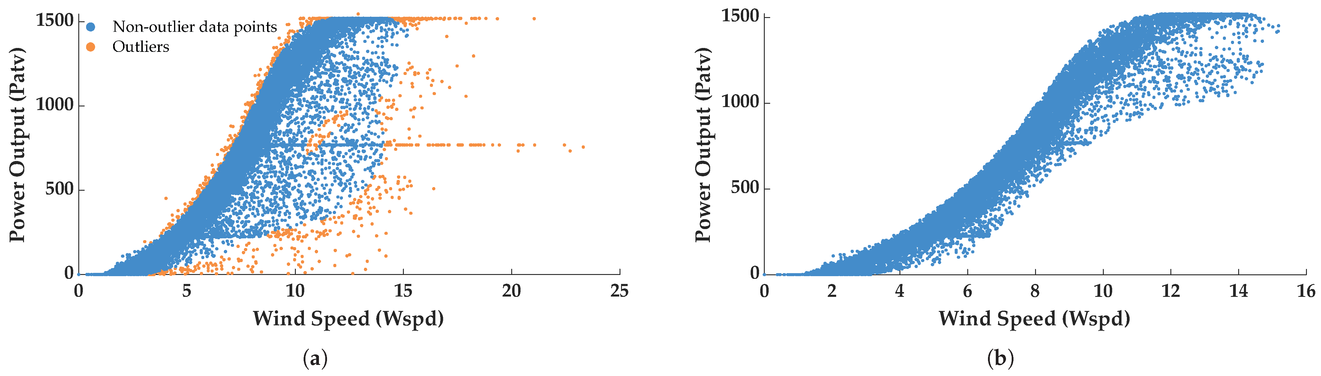
Next, we observed that some data points in the dataset may be due to measurement errors in the turbines, as well as degradation of the conversion efficiency of converting wind energy to electricity during certain time periods, or other external factors that would misrepresent the relational expression of wind speed to wind energy. Anomaly detection is performed using a One-Class Support Vector Machine (SVM) to identify and remove outliers, thus improving the accuracy and reliability of subsequent analysis and model training. Initially, all data points are labeled as normal (label = 1). To capture complex, non-linear data distributions, the Radial Basis Function (RBF) kernel is utilized. Additionally, prior to applying the One-Class SVM, the input data is normalized so that each feature has a mean of 0 and a variance of 1, ensuring that all features contribute equally to the anomaly detection process.

To define the proportion of outliers, a contamination rate of 10% is specified, which means that up to 10% of the data are assumed to consist of anomalies. The SVM of one class then assigns a score to each data point based on its deviation from the learning decision boundary-normal points typically receive positive scores, while outliers are assigned negative scores. A threshold of 0 is used to classify anomalies, so any data point with a score less than 0 is considered an outlier and subsequently removed. Figure 4a illustrates the dataset before outlier removal, with the orange points indicating the identified anomalies, and Figure 4b shows the cleaned data set that is used for further analysis.

The correlation analysis of the 134 wind turbine data is presented in Figure 5. A strong correlation was observed between Etmp and Itmp with a Pearson correlation coefficient of 0.89, indicating a significant thermal impact of the external environment on the interior of the turbine. However, this relationship is not relevant for wind energy prediction. In contrast, Wspd and Patv exhibit a strong correlation of 0.96, confirming that power generation is primarily driven by wind speed. Despite this, anomalies such as sensor malfunctions and transient inefficiencies can introduce deviations, highlighting the need for robust data pre-processing.

3.2. Cluster Analysis

In this subsection, the results of Modes-cluster and Turbines-cluster will be shown and analyzed.

3.2.1. Modes-Cluster

Since predicting wind speed trends solely based on a neural network model without prior knowledge is challenging, clustering trend terms provides structured a priori information that enhances the generalizability of the model. By categorizing trend terms, the model can better align its predictions with actual variations in wind speed, improving the accuracy of the prediction.

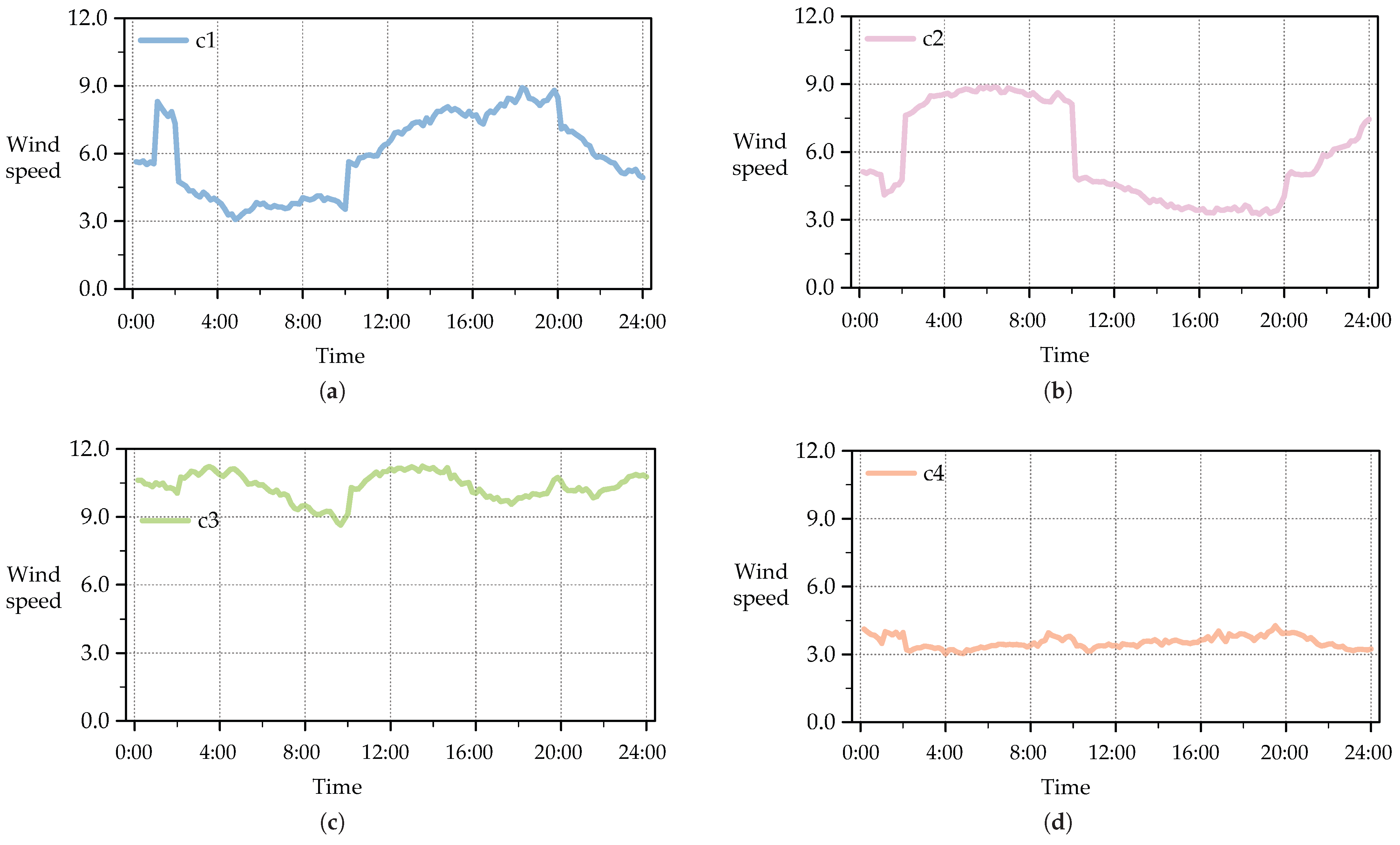
The results of the clustering in terms of days are shown in Figure 6. Since it does not make sense to analyze the clustering results of trends in days alone, analyzing the trends obtained by averaging the clustered trends is a better indication of the appropriateness of the number of categories. Figure 7 shows the resulting average wind speed trend patterns.

Figure 7 presents the wind speed patterns when the number of clusters is set to 4. The clustering results reveal distinct temporal patterns, which indicate that the dataset contains significantly different wind speed distributions throughout the day. The first category exhibits an early peak, followed by a gradual decline, suggesting a morning wind surge that stabilizes later. The second category features an evident increase in wind speed in the morning, followed by a midday decline and a secondary rise in the evening, potentially indicating the influence of thermal effects on wind dynamics. The third category represents consistently high wind speeds with minor fluctuations, which could be associated with stable meteorological conditions or high-altitude wind flow in specific regions. In contrast, the fourth category displays consistently low wind speeds with minimal variation, possibly linked to geographical factors such as sheltered areas or nighttime wind behavior.

These clustering results suggest that wind speed trends are not uniform but instead exhibit structured variability across different time periods and locations. The presence of distinct trend patterns emphasizes the need to classify the wind speed data before feeding them into predictive models. Without such classification, a neural network may struggle to learn meaningful relationships due to the overlapping nature of wind speed variations. By segmenting the data set into clear trend groups, the model can process data more effectively, leading to improved generalization and reduced uncertainty in wind power prediction. Additionally, the distinct wind patterns observed in Figure 7 confirm that choosing four clusters provides a reasonable balance between trend differentiation and computational efficiency, ensuring that the model captures essential wind speed behaviors while maintaining its predictive capacity.

3.2.2. Turbines-Cluster

Since the dataset of this paper consists of 134 wind turbines, and the geographic locations of the 134 wind turbines are not the same. If the 134 turbines are only clustered for wind speed trend to improve the generalization ability, it is not possible to tailor the model to the different geographic conditions of each turbine, by categorizing the 134 turbines, the model can be better predicted according to the different geographic conditions, thus improving the accuracy of the prediction.

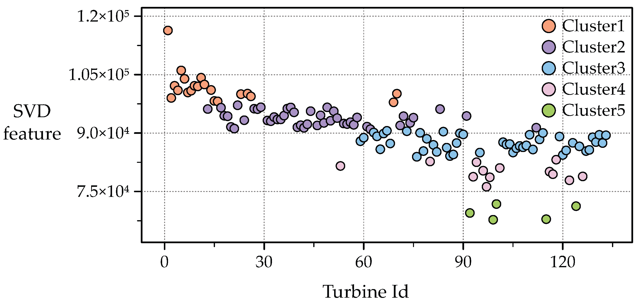
The clustering results for the wind turbines are shown in Figure 8. The clustering results show the differences in the SVD matrix values obtained for different wind turbines, and it is clear that there is no overlap in the range of SVD matrix values between the different classes of wind turbines. The SVD matrix values are generated by the correspondence between wind speed and wind energy, and different geographic locations can subtly affect the conversion of wind speed and wind energy. Therefore, the SVD matrix values can reflect the differences in geographical locations. The SVD matrix values here are only reflective of the geographic location, and the values themselves have no special meaning.

3.3. Experiment and Results

The experimental evaluation was carried out by comparing multiple neural network models in terms of the mean squared error (MSE), the root mean squared error (RMSE) and the coefficient of determination ($R^2$). The results are summarized in

Table 4. Parameter Error Statistics for MESN and comparative model.

Model	MSE	RMSE	R2	Training Time (s)
ANN	0.3523	0.5936 (2.23)	0.9709	36,102
BP	0.1889	0.4346 (1.63)	0.9844	4661
GRU	0.4166	0.6455 (2.42)	0.9617	59,203
LSTM	0.4270	0.6534 (2.45)	0.9607	62,628
RBF	0.1842	0.4292 (1.61)	0.9848	11,795
ESN	0.3194	0.5651 (2.12)	0.9736	2585
MESN	0.0711	0.2667 (1.00)	0.9905	2884

, and a visual comparison is provided in Figure 9 for better clarity. As observed in the table, the proposed MESN model substantially outperforms the other neural networks, achieving the lowest MSE and RMSE values while achieving the highest $R^2$, which is closest to 1. These results demonstrate the superior predictive capability and robustness of MESN. In terms of training time, the training time of ESN is the shortest, while the training time of MESN is just longer than that of ESN.This can prove that the computational efficiency of MESN is superior.

Figure 10 further illustrates the performance of MESN in the test data set, where the predicted values were compared with the actual values for the 8 days of the test set. The predicted values (blue) closely match the data of the test set (orange), confirming the exceptional accuracy and reliability of the model. The significant reduction in error and enhanced correlation with the ground truth validate the effectiveness of MESN in predicting wind speed. 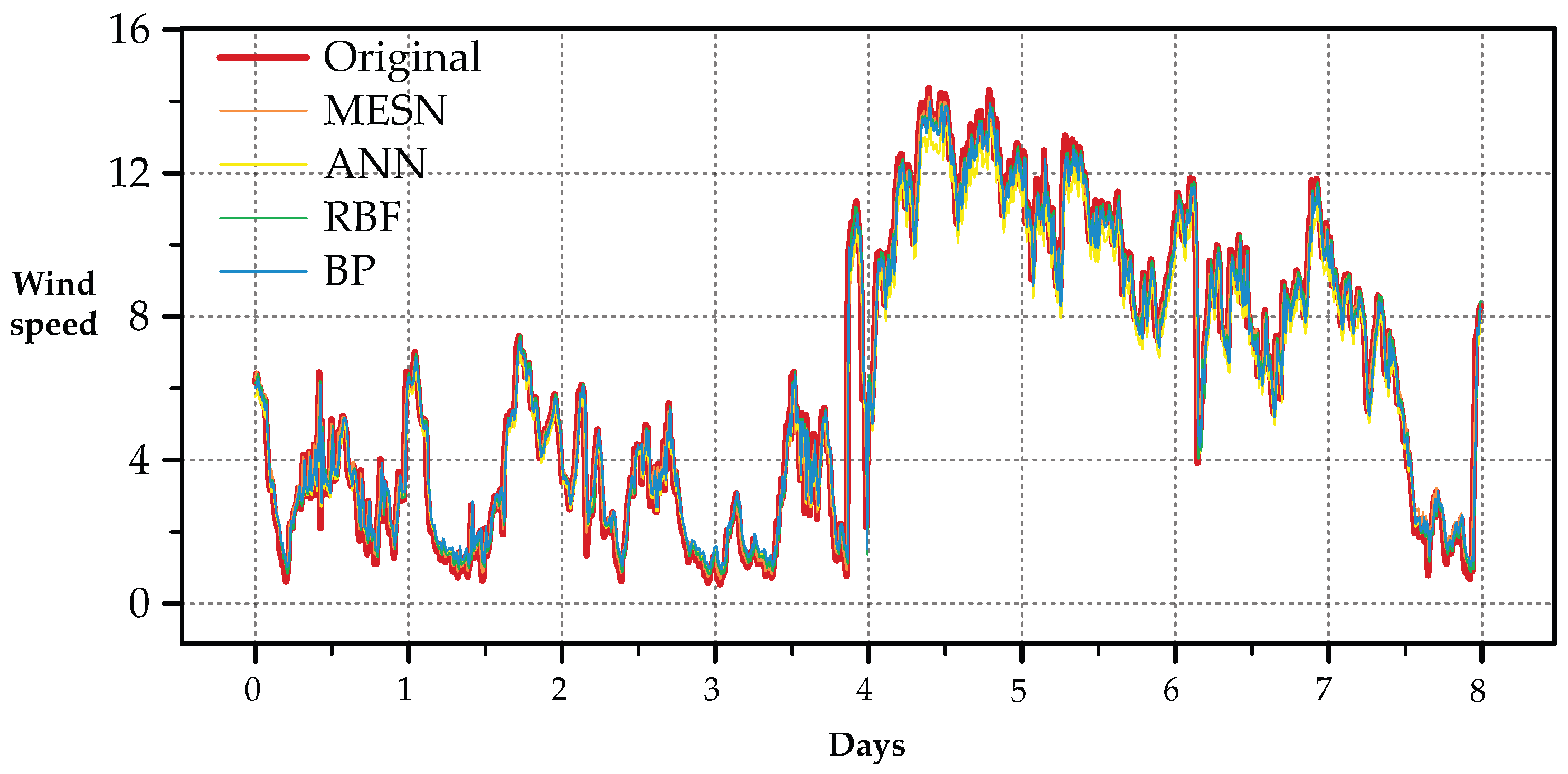Figure 11 compares the predictions of three of the better traditional models (ANN, BP, and RBF) with the actual values over the 8 days of the test set, and although MESN (orange) is not the model that best matches the data in the test set (red) for some tiny time periods, its overall prediction accuracy is the most accurate of all the models. These findings suggest that MESN provides a more precise and stable forecasting framework compared to traditional neural network models.

Finally, we converted the wind speed to wind energy and again compared the predicted values with the actual values for the 8 days of the test set. As shown in Figure 12, the predicted values (blue) are in good agreement with the data of the test set (red), indicating that MESN has practical applications in the wind power industry. The conversion equation is shown in (20). Given that the wind turbine’s output power is limited to a maximum of 1550 watts and a minimum of 0 watts, any predicted values exceeding 1550 watts were truncated at 1550, while values below zero were reset to zero watts.

$$Patv={\displaystyle \frac{1915}{1+e^{-0.445·(Wspd-7.52)}}}-150$$

(20)

where e is the natural constant, Patv is the output power, Wspd is the wind speed.

3.4. Sensitivity Analysis

Sensitivity analysis is the study of how uncertainty in the output of a model or system is partitioned and assigned to different sources of uncertainty in the input. In this subsection, sensitivity analyses are performed for the hyperparameters of the MESN model, and we perform univariate sensitivity analyses by varying the spectral radius, leakage rate, and reservoir size of the MESN within a reasonable range.

Table 5. Sensitivity analysis of MESN hyperparameters.

Spectral Radius	Leaking Rate	Reservoir Size	MSE	RMSE	R²	Case
0.70	0.250	100	0.0785	0.2802	0.9882	1
0.70	0.275	150	0.0753	0.2744	0.9889	2
0.70	0.300	200	0.0741	0.2722	0.9893	3
0.70	0.325	250	0.0756	0.2750	0.9888	4
0.70	0.350	300	0.0768	0.2771	0.9884	5
0.75	0.250	200	0.0748	0.2735	0.9891	6
0.75	0.275	150	0.0732	0.2706	0.9895	7
0.75	0.300	200	0.0715	0.2674	0.9902	8
0.75	0.325	250	0.0728	0.2698	0.9897	9
0.75	0.350	300	0.0739	0.2718	0.9893	10
0.80	0.250	300	0.0729	0.2700	0.9896	11
0.80	0.275	200	0.0713	0.2670	0.9903	12
0.80	0.300	200	0.0711	0.2667	0.9905	OP
0.80	0.325	150	0.0721	0.2685	0.9900	13
0.80	0.350	100	0.0735	0.2711	0.9894	14
0.85	0.250	250	0.0742	0.2724	0.9892	15
0.85	0.275	250	0.0725	0.2693	0.9898	16
0.85	0.300	200	0.0737	0.2715	0.9895	17
0.85	0.325	150	0.0749	0.2737	0.9891	18
0.85	0.350	100	0.0763	0.2762	0.9887	19
0.90	0.250	300	0.0756	0.2750	0.9889	20
0.90	0.275	200	0.0741	0.2722	0.9894	21
0.90	0.300	150	0.0753	0.2744	0.9890	22
0.90	0.325	100	0.0767	0.2770	0.9885	23
0.90	0.350	200	0.0779	0.2791	0.9881	24

where the bolded parts represent the optimal parameters.

shows the effects of changes in spectral radius, leaking rate and reservoir size within a reasonable range on the errors of the parameters used in this paper, respectively. It can be seen that the adjustment of spectral radius, leaking rate and reservoir size for MESN does not cause large fluctuations in the prediction error, indicating that the MESN model has a certain degree of stability, will not be due to the subtle changes in the hyper-parameters to produce a large prediction bias and the impact of the use of optimal The effect of the parameter error after using optimal parameters is the best. Through the data in the table, we can observe that the spectral radius should be controlled in the critical interval of 0.7 to 0.9. The Leaking Rate has a wide tolerance range, but it is best to keep it in the 0.275 to 0.325 range. Moreover, the Reservoir Size has a diminishing return phenomenon after more than 200 nodes. This characteristic makes MESN maintain a stable prediction performance even with certain parameter calibration errors when actually deployed, which significantly reduces the difficulty of parameter tuning for industrial applications.

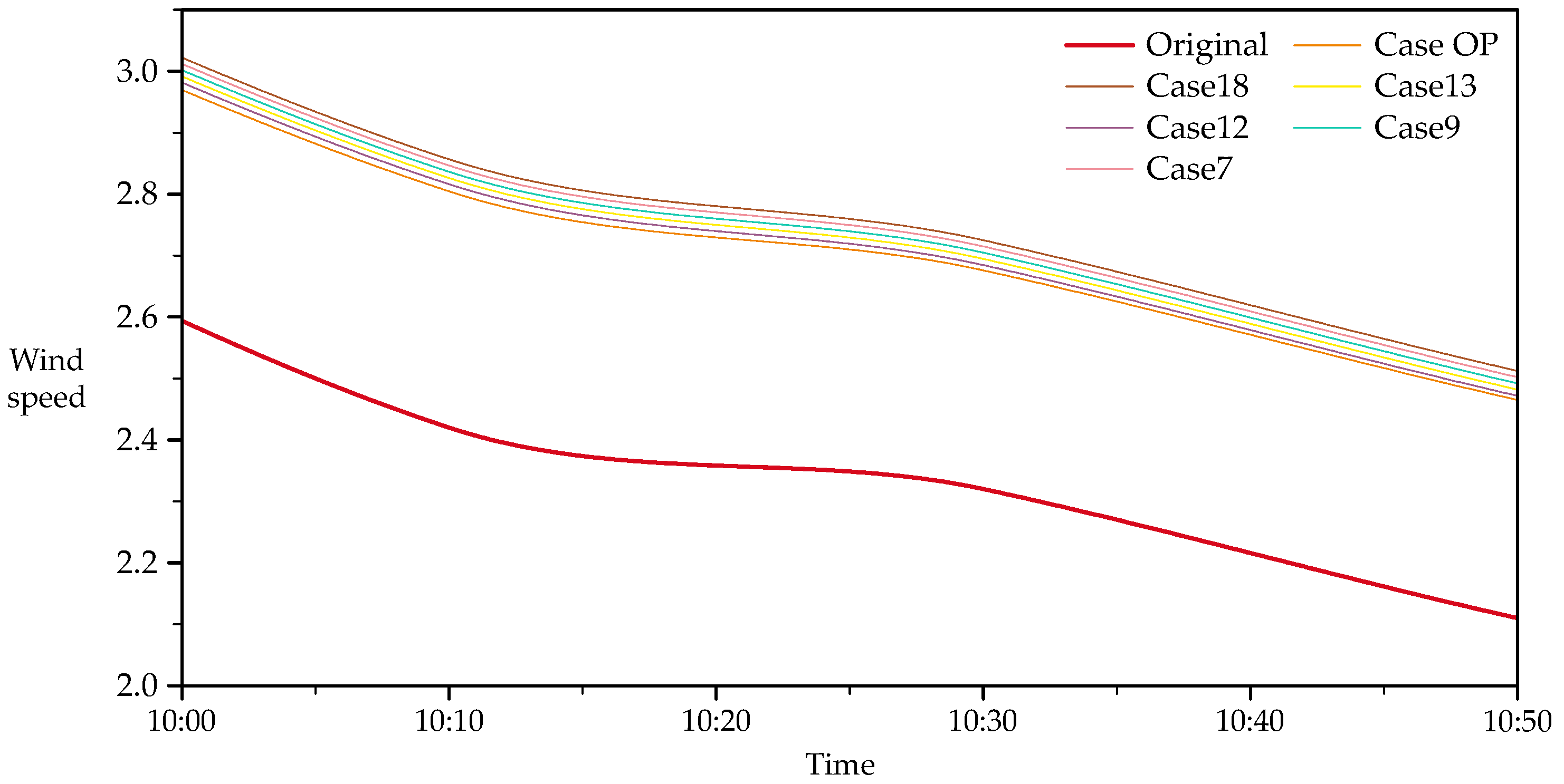
Figure 13 shows the sensitivity analysis of the prediction data generated by applying different hyperparameters to MESN, as the predicted values of some hyperparameters are too close to each other therefore the prediction data of only a few representative parameters are selected for presentation. It can be seen that under different hyperparameters, the prediction effect of MESN is more stable, with little up and down fluctuation, which can be considered that MESN has excellent robustness. Under the optimal parameters, the prediction effect of MESN is the best.

4. Conclusions

In this paper, we proposed a wind speed prediction model based on modularization and an Echo State Network (ESN). The model assigned specialized tasks to distinct modules and integrated a novel aggregation algorithm into the output integration module to effectively fuse diverse data categories. The modular design offered several key advantages. First, by decomposing the overall task into submodules, the model effectively captured unique features and patterns within different data segments, thereby reducing the risk of overfitting and enhancing robustness. Second, the modular approach enabled targeted optimization, and individual modules could be fine-tuned independently, allowing for seamless updates and adaptations to new data or changing environmental conditions. Third, the modular structure improved interpretability, as each module’s function was well-defined, making it easier to analyze the contribution of specific components to the overall prediction performance. Experimental comparisons with various neural networks demonstrated that our model minimized prediction errors and improved accuracy by an average factor of 2.08. Furthermore, converting wind speed predictions into wind energy estimates further validated its practical value in industrial applications.

However, although the model has achieved a high level of accuracy in the studied wind farms, its generalizability to the performance in datasets of increasing size or in large-scale wind farms still needs to be investigated, and about the potential optimization strategies, such as model pruning and parallel processing, and other methods can be discussed and optimized in future research, which will be the focus of the future research.