Overload Risk Assessment of Transmission Lines Considering Dynamic Line Rating

Abstract

Dynamic line rating (DLR) technology dynamically adjusts the current-carrying capacity of transmission lines based on real-time environmental parameters and plays a critical role in maximizing line utilization, alleviating power flow congestion, and enhancing the security and economic efficiency of power systems. However, the strong coupling between the dynamic capacity and environmental conditions increases the system’s sensitivity to multiple uncertainties and causes complications in the overload risk assessment. Furthermore, conventional evaluation methods struggle to meet the minute-level risk refresh requirements in ultrashort-term forecasting scenarios. To address these challenges, in this study, an analytical overload risk assessment framework is proposed based on the second-order reliability method (SORM). By transforming multidimensional probabilistic integrals into analytical computations and establishing a multiscenario stochastic analysis model, the framework comprehensively accounts for uncertainties such as component random failures, wind power fluctuations, and load variations and enables the accurate evaluation of the overload probabilities under complex environmental conditions with DLR implementation. The results from this study provide a robust theoretical foundation for secure power system dispatch and optimization using multiscenario coupled modeling. The effectiveness of the proposed methodology is validated using case studies on a constructed test system.

1. Introduction

With the large-scale integration of renewable energy sources such as wind and photovoltaic power, power systems face the dual challenges of operational flexibility and transmission capacity constraints [1]. Traditionally, the capacity of transmission lines is determined by the maximum allowable current-carrying capacity, and this capacity depends on the maximum permissible operating temperature and environmental parameters [2]. In current grid dispatch practices, the static line rating (SLR) method, which is based on extreme environmental conditions, is prevalent for evaluating transmission line limits [3]. However, this conservative approach fails to fully exploit the actual transmission potential under real-world operating conditions [4], resulting in the underutilization of line capacities in variable environments [5].

To address these limitations, dynamic line rating (DLR) technology has emerged as an innovative solution [6]. By leveraging real-time meteorological data at transmission line locations, DLR dynamically calculates the thermal capacity limits to more accurately reflect actual transmission capabilities [7]. This technology enables cost-effective expansion of transmission potential within existing infrastructure [8], particularly enhancing renewable energy utilization in systems with high penetration of intermittent wind and solar power [9,10].

The dynamic nature of DLR essentially transforms transmission capacity from a deterministic parameter to an environment-dependent stochastic variable [11]. While DLR offers operational advantages in power system optimization, the inherent uncertainty in transmission capacity becomes deeply embedded in system operations [12], necessitating rigorous risk assessment methodologies. Accurate overload risk assessment becomes crucial for maximizing DLR benefits while ensuring system reliability. Existing studies [13,14,15] have attempted to model uncertainties through box-type uncertainty sets or data-driven fuzzy sets to address the correlations between the wind power output and line capacity. However, these approaches predominantly focus on single-system-state evaluations and inadequately address the dynamic overload risks across multiple operational scenarios [16].

Current research reveals that systems operating at DLR-enhanced high-load states exhibit significantly reduced buffer margins against contingencies [17]. In ultrashort-term operation scenarios, cascading effects may emerge from sudden wind speed drops, causing capacity contraction and power transfer path interruptions [18]. Traditional single-scenario risk assessment models tend to substantially underestimate these overload risks, necessitating comprehensive multistate evaluations to inform power system dispatch decisions [19]. However, the risk assessment of dynamic rating technologies faces heightened real-time requirements at minute-level ultrashort-term time frames. The inherent volatility of DLR-derived transmission capacity creates critical computational challenges—conventional methods such as Monte Carlo simulations prove prohibitively time-consuming for rapid risk refreshment cycles [20]. This technological gap underscores the urgent need for innovative assessment methodologies that combine analytical rigor with computational efficiency. While recent studies have proposed data-driven methods that consider topological changes [21] and modified failure probability models that incorporate line degradation [22], these methods remain inapplicable to DLR-integrated systems.

Existing studies have addressed SLR’s conservatism [3,4,5], advanced DLR’s real-time adaptability [6,7,8,9,10], and explored uncertainty modeling in risk assessment [13,14,15]. However, these efforts predominantly focus on single-scenario evaluations, lack computational efficiency for ultrashort-term frameworks [16,20], and fail to integrate multiscenario stochasticity with component failures. This gap motivates our proposed analytical framework, which unifies DLR-driven dynamic capacity, multiscenario uncertainties, and second-order reliability methods to enable rapid and accurate overload risk assessment.

To resolve these issues, in this study, a DLR technology model is established to analyze the transmission capacity variation patterns under different meteorological conditions (temperature, wind speed, and solar radiation) and load levels. We subsequently construct a multiscenario stochastic analysis framework that incorporates uncertainties from component failures, wind power fluctuations, and load variations. Finally, second-order surface approximation methods are employed to evaluate the overload risk indices for each scenario. The comprehensive risk assessment results provide operational guidance for power system dispatch and optimization.

2. Overload Criterion of Transmission Line Based on the Dynamic Capacity Increase Calculation Model

2.1. Model Building

During operation, the conductor temperature of transmission lines is primarily determined by three key factors: the magnitude of current flowing through the conductor, its intrinsic electrical characteristics (including cross-sectional area and resistance), and ambient environmental conditions such as ambient temperature, wind speed, wind direction, and solar radiation. As standardized in IEEE Std. 738 [2], the steady-state thermal equilibrium model for overhead transmission lines can be mathematically expressed by Equation (1):

$${\rho }_l{\displaystyle \frac{\Delta {\varphi }_{l,t}}{\Delta t}}=I_{l,t}^2{R}_{l,t}+q_{l,t}^{\mathrm{s}}-q_{l,t}^{\mathrm{c}}-q_{l,t}^{\mathrm{r}},$$

(1)

where ${\rho }_l$ represents the specific heat capacity of the transmission line l; ${\varphi }_{l,t}$ denotes the temperature of line l at time t; $\Delta$ represents the incremental change in the corresponding variable; $I_{l,t}$ represents the current flowing through line l at time t; $R_{l,t}$ and $q_{l,t}^{\mathrm{s}}$ denote the resistance and solar heat gain of line l at time t, respectively; and $q_{l,t}^{\mathrm{r}}$ and $q_{l,t}^c$ represent the radiative cooling and convective cooling (assuming the presence of natural wind) of line l at time t, respectively.

This equation captures the dynamic interplay between the electrical and thermal parameters and provides a comprehensive framework for evaluating the thermal behavior of transmission lines under varying operational and environmental conditions.

When the conductor temperature reaches the maximum permissible long-term operating temperature ${\theta }_c$, a thermal equilibrium state is achieved where the heat absorption power equals the heat dissipation power. This balance can be expressed using the thermal equilibrium equation, from which the dynamic line rating limit $I_{l,t}^{DLR}$ of the transmission line can be derived as follows:

$${\left(I_{l,t}^{DLR}\right)}^2{R}_c+q_{l,t}^{\mathrm{s}}=q_{l,t}^{\mathrm{c}}+q_{l,t}^{\mathrm{r}},$$

(2)

$$I_{l,t}^{DLR}={\displaystyle \frac{\sqrt{q_{l,t}^{\mathrm{c}}+q_{l,t}^{\mathrm{r}}-q_{l,t}^{\mathrm{s}}}}{\sqrt{R_{\mathrm{c}}}}},$$

(3)

where $R_{\mathrm{c}}$ represents the conductor resistance at the maximum permissible long-term operating temperature ${\varphi }_{\mathrm{c}}$.

To establish the relationship between the dynamic line rating (DLR) limit $I_{l,t}^{DLR}$ and the environmental parameters, the variables for solar heat gain $q_{l,t}^{\mathrm{s}}$, convective cooling $q_{l,t}^c$, and radiative cooling $q_{l,t}^{\mathrm{r}}$ are analytically expressed as functions of the ambient environmental conditions along the transmission line. Specifically, the radiative cooling $q_{l,t}^{\mathrm{r}}$ can be expressed as follows:

$$q_{l,t}^{\mathrm{r}}=5.67\times {10}^{-8}\pi k_{\mathrm{e}}{D}_l({\varphi }_c^4-T_{l,t}^4),$$

(4)

where $D_l$ represents the conductor diameter; $T_{l,t}$ denotes the ambient temperature at the location of line l at time t; and $k_{\mathrm{e}}$ is the emissivity of the conductor surface.

In this study, the presence of natural wind is considered, and the influence of the wind direction on the conductor cooling efficiency is neglected. Under these assumptions, the convective cooling $q_{l,t}^{\mathrm{c}}$ can be expressed as follows:

$$q_{l,t}^{\mathrm{c}}=\pi {\lambda }_{l}E{U}_{l,t}({\varphi }_{\mathrm{C}}-T_{l,t}),$$

(5)

$$E{U}_{l,t}=0.65R_{\mathrm{e}}^{0.2}+0.23R_{\mathrm{e}}^{0.61},$$

(6)

$$R_{\mathrm{e}}=1.644\times {10}^9{\nu }_{l,t}{D}_l[T_{l,t}+0.5({\varphi }_{\mathrm{C}}-T_{l,t})){]}^{-1.78},$$

(7)

where ${\lambda }_l$ represents the convective heat transfer coefficient of the air film in contact with transmission line l; $E{U}_{l,t}$ denotes the Nusselt number; $R_{\mathrm{e}}$ is the Reynolds number; and ${\nu }_{l,t}$ represents the wind speed at the location of line l at time t.

The solar heat gain $q_{l,t}^{\mathrm{s}}$ is calculated as follows:

$$q_{l,t}^{\mathrm{s}}={\gamma }_l{S}_{l,t}{D}_l,$$

(8)

where $\gamma$ represents the absorption coefficient of the transmission line, and $S_{l,t}$ denotes the solar irradiance at the location of line l at time t.

Given fixed transmission line parameters and configurations, the dynamic line rating limit $I_{l,t}^{DLR}(X)$ is governed primarily by a set of stochastic variables X = {$v_{l,t},S_{l,t},T_{l,t}$}, where $v_{l,t}$, $S_{l,t}$, and $T_{l,t}$ correspond to the wind speed, solar radiation intensity, and ambient temperature, respectively.

The overload criterion g(X) for the transmission line can be formulated as follows:

$$g(X)=I_{l,t}^{DLR}(X)-\left|I_{l,t}\right|,$$

(9)

where $I_{l,t}$ represents the actual current-carrying capacity of the transmission line. The use of absolute values is intended to disregard the direction of current flow and to focus solely on whether the line current exceeds its safe operational limit.

The actual current-carrying capacity $I_{l,t}$ is determined by constraints (10)–(17).

The generator output constraints are as follows:

$$P_g^{\min }\le p_{g,t}\le P_g^{\max }\hspace{1em}\hspace{1em} \forall g, \forall t,$$

(10)

where $P_g^{\min }$ and $P_g^{\max }$ represent the lower and upper limits of the power output for generator g, respectively.

The generator ramp rate constraints are as follows:

$$p_{g,t+1}-p_{g,t}\le R_g^{+}{u}_{g,t}+P_g^{\max }(1-u_{g,t})\hspace{1em}\hspace{1em}\forall g, \forall t,$$

(11)

$$p_{g,t}-p_{g,t+1}\le R_g^{-}{u}_{g,t+1}+P_g^{\max }(1-u_{g,t+1})\hspace{1em}\hspace{1em}\forall g, \forall t,$$

(12)

where $R_g^{+}$ and $R_g^{-}$ represent the positive and negative ramp rates of generator g, respectively.

The reference node phase angle constraint is as follows:

$${\theta }_{\mathrm{ef},t}=0\hspace{0.33em}\hspace{0.33em}\hspace{0.33em} \forall t,$$

(13)

where ${\theta }_{\mathrm{ef},t}$ represents the phase angle at the reference node during time period t.

The DC power flow-based line power flow is as follows:

$$p_{l,t}=B_{n_1,n_2}({\theta }_{n_1}-{\theta }_{n_2})\hspace{0.33em}\hspace{0.33em}\hspace{0.33em} \forall l,\forall t,$$

(14)

where $B_{n_1,n_2}$ represents the admittance of the transmission line; ${\theta }_{n_1}$ and ${\theta }_{n_2}$ denote the phase angles at nodes n₁ and n₂, respectively, during time period t; and n₁, n₂ ∈ N_l, where N_l is the set of nodes connected to transmission line l.

The power system node balance constraint is as follows:

$${\displaystyle \sum _{g\in {\mathrm{\Omega }}_g(n)}{p}_{gt}}+{\displaystyle \sum _{w\in {\mathrm{\Omega }}_w(n)}{p}_{wt}}+{\displaystyle \sum _{l\in {\mathrm{\Omega }}_{O_2}(n)}{p}_{lt}}-{\displaystyle \sum _{l\in {\mathrm{\Omega }}_{O_1}(n)}{p}_{lt}}-{\displaystyle \sum _{d\in {\mathrm{\Omega }}_d(n)}{p}_{dt}}=0,\forall n,\forall t.,$$

(15)

where ${\mathrm{\Omega }}_g(n)$, ${\mathrm{\Omega }}_w(n)$, ${\mathrm{\Omega }}_{O_2}(n)$, ${\mathrm{\Omega }}_{O_1}(n)$, and ${\mathrm{\Omega }}_d(n)$ represent the sets of generator g, wind turbine generator w, incoming transmission lines O₁, outgoing transmission lines O₂, and load lines d connected to the power system node n, respectively; and $p_{dt}$ denotes the power of the load line d during time period t.

The transmission line current-carrying capacity constraint is as follows:

$$-I_{l,t}^F\le I_{l,t}\le I_{l,t}^F\hspace{0.33em}\hspace{0.33em}\hspace{0.33em} \forall l,\forall t,$$

(16)

where $I_{l,t}^F$ represents the dynamic line rating limit of transmission line l at time t, which is determined through predictive adjustments.

The system reserve constraint is as follows:

$$Q_t=0.03\cdot {\displaystyle \sum _n^N{P}_{n,t}^{\mathrm{d},\mathrm{fore}}}+0.05\cdot {\displaystyle \sum _w^{N_W}{P}_{w,t}^{\mathrm{fore}}},$$

(17)

The total system reserve is typically determined based on deterministic criteria such as the “N-1” rule or the “3 + 5” rule. In this study, the “3 + 5” rule is adopted, where the total reserve is set to 3% of the load forecast plus 5% of the wind power output forecast.

In general, transmission lines span long distances, and the meteorological conditions influencing their DLR limits vary along their lengths. In practice, weather monitoring devices can be strategically placed along lines according to specific trends [22]. Using Equation (3), the DLR limit for each segment of a line can be determined, and the minimum value among these segments is selected as the DLR limit for the entire line during that time period.

To calculate the probability of overload occurrence, we assume that the random vector $X={(v_{l,t},S_{l,t},T_{l,t})}^T$ has a joint probability density function k(x). The probability of line l at time t, overload $P_{f,l,t}$ can then be defined using an n-dimensional integral:

$$P_{f,l,t}=P(x\in {\mathrm{\Omega }}_F)={\displaystyle {\int }_{{\mathrm{\Omega }}_F}k}(x)dx,$$

(18)

where x represents a specific realization of the random vector $X={(v_{l,t},S_{l,t},T_{l,t})}^T$; g(x) partitions the n-dimensional probability space into a safe region ${\mathrm{\Omega }}_S$ = {x: g(x) > 0} and a failure region ${\mathrm{\Omega }}_F$ = {x: g(x) ≤ 0}; and Ω_F denotes the failure region described by the line overload criterion function g(x) and indicates the occurrence of a line overload.

However, when the number of random variables n is greater than or equal to 3, the n-dimensional integral in the probability calculation becomes computationally challenging owing to the lack of a closed-form solution. To address this, approximate methods can be employed to evaluate the probability integral. These methods not only increase computational efficiency but also maintain a high level of accuracy.

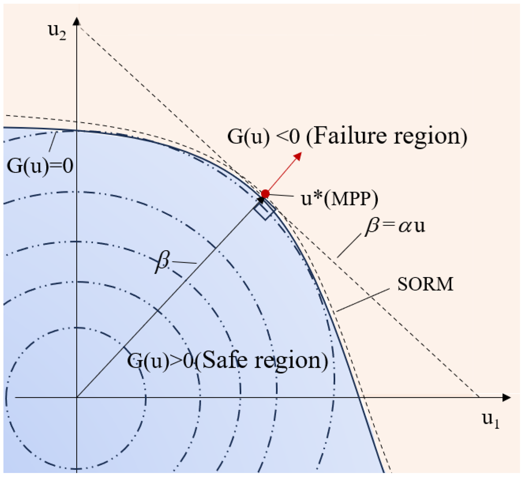
2.2. Overload Probability Solution Based on Second-Order Surface Approximation

To address the challenge of directly solving the multidimensional integral of the overload criterion over the failure region in the presence of multiple random variables, the second-order reliability method (SORM) is used. This approach transforms the original random variables into a standard normal space and converts the complex non-normal distribution problem into a standard normal distribution problem. In the standard normal space, the probability of the failure region is estimated using the most probable point (MPP) of failure and curvature information, thereby avoiding the direct computation of complex integrals. The algorithmic principle is illustrated in Figure 1.

By employing the Nataf transformation, the random variable vector $X={(v_{l,t},S_{l,t},T_{l,t})}^T$ is converted into a standard normal distribution $U={(u_1,u_2,u_3)}^T$, thereby mapping the random variables from the original space to the standard normal space. In the standard normal space, the overload criterion function $G(u)$ is subsequently simplified using a first-order Taylor expansion:

$$G(u)\approx {\displaystyle \sum _{i=1}^n{\left.\frac{\partial G}{\partial u_i}\right|}_{u=u^{*}}}(u_i-u_i^{*})=\Vert \nabla G(u^{*})\Vert \left(\beta -\alpha {\displaystyle \sum _{i=1}^n{u}_i}\right),$$

(19)

where $\nabla G(u*)$ represents the row vector of the gradient, which linearizes the failure domain $G\left(u\right)\le 0$, i.e., the half-space defined by $\beta -\alpha {\displaystyle \sum _{i=1}^n{u}_i}\le 0$. The reliability index $\beta =\alpha {\displaystyle \sum _{i=1}^n{u}_i*}$ is defined as the minimum distance from the origin to the limit state surface in the standard normal space, and $\alpha$ represents the normalized negative gradient vector at the design point. u* is the MPP on the boundary of the overload criterion function $G(u)=0$ and represents the point most likely to lead to failure.

In the standard normal space, the MPP is the point on the failure boundary that is closest to the origin. This shortest distance is known as the reliability index β:

$$\beta =\sqrt{{\displaystyle \sum _{i=1}^n{u}_i^2}}={\displaystyle \frac{{\left|{\displaystyle \sum _{i=1}^n\frac{\partial G}{\partial u_i}}\right|}_{u=u^{*}}{u}_i^{*}}{\sqrt{{\displaystyle \sum _{i=1}^n{\left(\frac{\partial G}{\partial u_i}{|}_{u=u^{*}}\right)}^2}}}},$$

(20)

The MPP is obtained by solving a constrained optimization problem, defined as follows:

$$\arg {\min }_{u*}\{\Vert u\Vert | G(u)=0\},$$

(21)

The above optimization problems are solved to determine the MPP points and the minimum distance.

Without considering the curvature effects of the overload criterion function $G(u)$, the overload probability can be initially approximated as follows:

$$P_{f,l,t}\approx \mathrm{\Phi }(-\beta ),$$

(22)

where $\mathrm{\Phi }(\cdot )$ denotes the cumulative distribution function of the standard normal distribution.

After the design point is obtained, the second-order reliability method (SORM) performs a second-order Taylor expansion of the overload criterion function around the MPP and constructs a more accurate surface approximation to calculate the overload risk. By incorporating the Hessian matrix and solving for the curvature values, the SORM provides an enhanced approach to a reliability assessment and is particularly suitable for systems with significant nonlinearities.

In the quadratic surface approximation method, the Taylor series expansion of the overload criterion function at the standard normal space $u^{*}$ is considered as follows:

$$G(u)\cong \Vert \nabla G(u^{*})\Vert \left(\beta -\alpha {\displaystyle \sum _{i=1}^n{u}_i}\right)+{\displaystyle \frac{1}{2}}{\displaystyle \sum _{i=1}^n{\displaystyle \sum _{j=1}^n\frac{{\partial }^{2}G}{\partial u_i\partial u_j}}}{|}_{u=u^{*}}(u_i-u_i^{*})(u_j-u_j^{*}),$$

(23)

$$\nabla G(u*)={\nabla }_{u*}G(u*)=(\partial G/\partial u_1^{*},\partial G/\partial u_2^{*},\dots ,\partial G/\partial u_n^{*}),$$

(24)

$$\alpha =-{\displaystyle \frac{\nabla G(u^{*})}{\Vert \nabla G(u^{*})\Vert }}=-{\displaystyle \frac{{\displaystyle \sum _{i=1}^n\frac{\partial G}{\partial u_i}}{|}_{u=u^{*}}}{\sqrt{{\displaystyle \sum _{i=1}^n{\left(\frac{\partial G}{\partial u_i}{|}_{u=u^{*}}\right)}^2}}}},$$

(25)

Considering the use of an orthogonal normalization matrix P, which rotates the coordinate axes such that $u^{\prime }=Pu$ and the design point lies on the $u_n^{\prime }$-axis (i.e., $u^{*}$ = ($u_1^{*}$, 0, …, 0)). The overload criterion function can be expressed as follows:

$$G^{\prime }(u^{\prime })=\beta -u_n^{\prime }+{\displaystyle \frac{1}{2\Vert \nabla G(u^{*})\Vert }}{\displaystyle \sum _{i=1}^n{\displaystyle \sum _{l=1}^n\left[{\displaystyle \sum _{k=1}^n\left({\displaystyle \sum _{j=1}^n{p}_{ij}}\frac{{\partial }^{2}G}{\partial u_j\partial u_k}{|}_{u=u^{*}}\right)}{p}_{lk}\right]}}(u_i^{\prime }-u_i^{\prime *})(u_l^{\prime }-u_l^{\prime *}),$$

(26)

where ${u^{\prime }}_n=\alpha P^{\mathrm{T}}u$. Through appropriate linear transformations and diagonalization, the overload criterion function is simplified as follows:

$$G^{\prime }(u^{\prime })=\beta -u_n^{\prime }+{\displaystyle \frac{1}{2}}{\displaystyle \sum _{i=1}^{n-1}{\kappa }_i}{u}_{i^{″}}^2,$$

(27)

where k_i denotes the eigenvalues of submatrix D11.

Following Breitung’s method [23], the overload probability $P_{f,l,t}$ is derived as follows:

$$P_{f,l,t}\approx \mathrm{\Phi }(-\beta ){\displaystyle \prod _{i=1}^{n-1}\frac{1}{\sqrt{1+\beta {\kappa }_i}}},$$

(28)

where β is the reliability index and Φ(·) represents the cumulative distribution function (CDF) of the standard normal distribution. Therefore, the overload probability can be expressed analytically as a function of the reliability index.

3. Overload Risk Assessment of Transmission Lines Based on Multiscenario Stochastic Analysis

In the context of increasing operational uncertainties in power systems, the stochastic failure of electrical equipment within system components and the fluctuations in the power load and renewable energy output are the primary uncertain factors affecting the ampacity of transmission lines. Thus, continuous prediction and risk assessment are needed, and greater demands on the risk assessment analysis of power system overloads are imposed. However, current operational risk assessments that consider dynamic line rating (DLR) do not account for multiple uncertainty scenarios; thus, it is impossible to evaluate system behavior under varying line environments, renewable energy outputs, and load changes.

In response, an overload risk assessment model is proposed based on scenario analysis. By integrating component random outage events with renewable energy output and load scenarios, a multiscenario framework for power system overload risk assessment is introduced. This framework calculates the overload risk indicators for each operational period of the system and assesses the overload risk level that considers the operational scenarios of the power system.

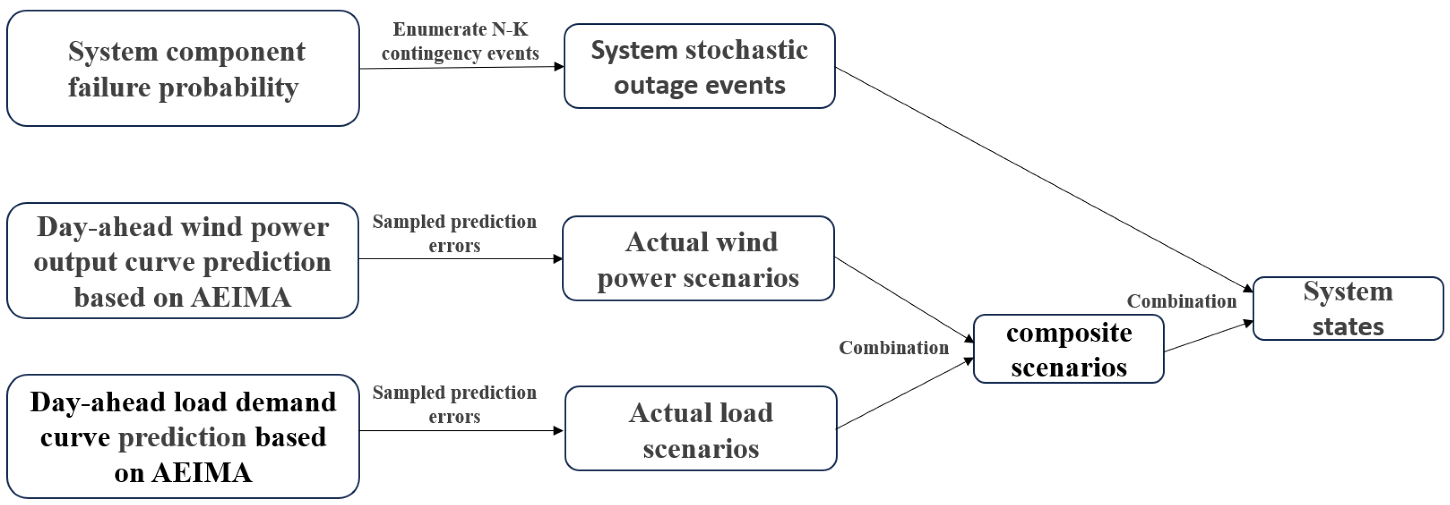
3.1. System State Generation and Uncertainty Modeling

The generation of system states is a crucial step in the assessment of transmission line overload risk within a power system. These system states encompass the availability status of components, as well as the actual wind power output scenarios and real load scenarios. Therefore, by integrating component random outage events with renewable energy output and load scenarios, the various states that the system may encounter during operation can be generated. This comprehensive approach ensures a robust evaluation of potential overload risks, considering the dynamic interplay between equipment reliability and the variability of renewable energy sources and consumer demand.

System components, which may include transmission lines, transformers, or generator units, have a failure rate that can be expressed as follows:

$$FOR={\displaystyle \frac{\lambda }{\lambda +\mu }},$$

(29)

where λ and μ represent the failure rate and repair rate of the equipment, respectively, and can be derived from historical data.

The system component failure probability model employs a two-state Markov model to generate the availability states of all components, thereby forming the system’s random outage events. In a random fault event k, which is generated by enumeration or sampling methods, the states of transmission lines and generator units $z_{l,k}$, $z_{\mathrm{g},k}$ are included. Using a transmission line as an example, the availability state $z_{l,k}$ is assigned a value of 0 if line l is in an unavailable state due to a forced outage and a value of 1 if it is in an available state.

The probability of a random outage event ${\pi }_k$ is given by the following:

$${\pi }_k={\displaystyle \prod _{i\in {\mathrm{\Psi }}_{k,up}}(1-FO{R}_i^0)}\cdot {\displaystyle \prod _{j\in {\mathrm{\Psi }}_{k,down}}F}O{R}_j^0,$$

(30)

where ${\mathrm{\Psi }}_{k,up}$ and ${\mathrm{\Psi }}_{k,down}$ represent the sets of available and unavailable components, respectively, corresponding to event k.

Owing to the inherent volatility and randomness in the prediction of renewable energy output and load, the renewable energy output and load at each time point are challenging to analytically express. Therefore, in operational reliability analysis, time series models are often employed to model renewable energy output. By integrating the forecast values and prediction errors, the time series output or load values for renewable energy stations are obtained as follows:

$$P_{t,s}^{\mathrm{RT}}=P_t^{\mathrm{fore}}+{\epsilon }_{t,s},t=1,2,3,\dots 24,$$

(31)

where the predicted value $P_t^{\mathrm{fore}}$ is integrated via quantile regression-based probabilistic forecasts, dynamically adjusting to spatial and temporal variability along transmission lines [24]. In this study, the wind speed and load are predicted using the AEIMA model [25]. Wind power and load prediction errors are modeled using Gaussian and skewed distributions (e.g., Cauchy and beta distributions), explicitly capturing tail risks associated with extreme deviations [26,27,28]. The prediction error for scenario s is labeled as ${\epsilon }_{t,s}$.

Considering the prediction errors of renewable energy output and load, the composite scenarios formed by renewable energy and load encompass a vast number of scenarios. Furthermore, to increase computational efficiency, the K-means clustering method [29] is employed to cluster the composite scenarios of the wind speed and load. The K-means algorithm reduces the dimensionality of composite scenarios while preserving critical uncertainty patterns, ensuring computational tractability without sacrificing key risk profiles.

The system state probability ${\pi }_{k,s}$, corresponding to the random outage event k and the composite scenario s, is obtained as follows:

$${\pi }_{k,s}={\pi }_s\cdot {\pi }_k,$$

(32)

where ${\pi }_s$ and ${\pi }_k$ represent the probabilities of the composite scenario s and the outage event k, respectively.

The system state generation process can be viewed as a coupling of probabilities in two dimensions: On one hand, the random outage event set is generated based on the component reliability model, with the outage event probabilities quantified by Equation (30). On the other hand, considering the uncertainty in renewable energy output and load forecasting, composite scenarios are constructed through time-series modeling and error sampling. These two probability spaces are mapped through joint probability in Equation (32), forming the complete system state set (k, s) that encompasses both equipment failures and operational uncertainties. The generation process is illustrated in Figure 2.

For a transmission line l, the probability of overload in the system state (k, s) is denoted as $P_{f,l,t}^{k,s}$. Consequently, the expected overload probability $P_{f,l,t}^{sw}$ for line l across multiple scenarios is given by the following:

$$P_{f,l,t}^{s\mathrm{w}}={\displaystyle \sum _k{\displaystyle \sum _s{\pi }_{k,s}\cdot }}{P}_{f,l,t}^{k,s}$$

(33)

3.2. Overload Risk Assessment Process Based on Scenario Analysis

The proposed overload risk assessment model based on scenario analysis in this paper follows the following workflow:

(1)

Based on the predicted curves and prediction errors of renewable energy output and load, scenarios for renewable energy and load are generated.

(2)

Using the system component failure probability model, the outage events for system components are generated.

(3)

The renewable energy and load scenarios are combined with the system component outage events to generate system states and their corresponding probabilities.

(4)

Power flow analysis is performed based on the system states and environmental parameters along the transmission lines. Second-order reliability methods are used to analytically calculate the expected overload probability indicators for the transmission lines.

4. Case Study

4.1. Parameter Setting

In this study, the modified IEEE-RTBS 6-node system and the IEEE-RTS79 system are employed to validate the correctness and effectiveness of the proposed model. The topological structure of the modified IEEE-RTBS 6-node system is illustrated in Figure 3. The modified IEEE-RTBS 6-node test system configuration is summarized in

Table 1. Parameters of the wind generator.

Wind Turbine Access Node	Installed Capacity (MW)
1	250
3	150

. The simulations are conducted on the MATLAB 2020a platform, which uses a computer equipped with a 3.0 GHz Intel^® Core™ i5 CPU (manufactured by Intel Corporation, Santa Clara, CA, USA) and 16 GB of RAM (the manufacturer may vary depending on the RAM brand, but the system was assembled commercially). Given the absence of wind farms in the original test systems, two wind turbine generators are incorporated, and the connected wind farm integration line spans approximately 30 km.

The modified IEEE-RTBS 6-node test system consists of 6 buses, 9 transmission lines, 11 thermal power units, 2 wind turbine generators, and 5 load points. The total installed capacity of the generation units is 1015 MW, with a peak load demand of 740 MW.

The load model of the test system adopts the daily demand curve from the IEEE-RBTS. The capacity and reliability parameters of the system components are detailed in

Table 2. Capacities and reliability parameters of the modified IEEE RBTS.

Component	Capacity (MW)	λ (Occ./Yr)	μ (Occ./Yr)	FOR0
Generator 1	45	2	194.67	0.0300
Generator 2	45	2	194.67	0.0350
Generator 3	60	4	194.67	0.0250
Generator 4	60	2.4	194.67	0.0350
Generator 5	60	1	219.27	0.0150
Generator 6	60	12	219.27	0.0150
Generator 7	45	2.4	159.27	0.0200
Generator 8	60	5	194.67	0.0150
Generator 9	60	3	146.00	0.0150
Generator 10	60	6	194.67	0.0150
Generator 11	60	6	194.67	0.0150
Line 1	81	1.5	876.00	0.0017
Line 2	81	5	876.00	0.0057
Line 3	71	4	876.00	0.0045
Line 4	71	1	876.00	0.0011
Line 5	71	1	876.00	0.0011
Line 6	71	1.5	876.00	0.0017
Line 7	71	5	876.00	0.0057
Line 8	71	1	876.00	0.0011
Line 9	71	1	876.00	0.0011

. To simplify the computational complexity, the maximum number of concurrent outages is set to 3. The system encompasses a total of 1351 “N-3” contingency events. To reduce the computational burden, the analysis considers all “N-1” scenarios, as well as the top 10 most probable “N-2” and “N-3” events based on their failure probabilities.

The environmental parameters along the line are predicted by the probability prediction method based on quantile regression used in the literature [30]. The data from the micrometeorological instruments installed in each area are treated as independent datasets to predict the probability distributions of the environmental parameters along the transmission line in each area every hour.

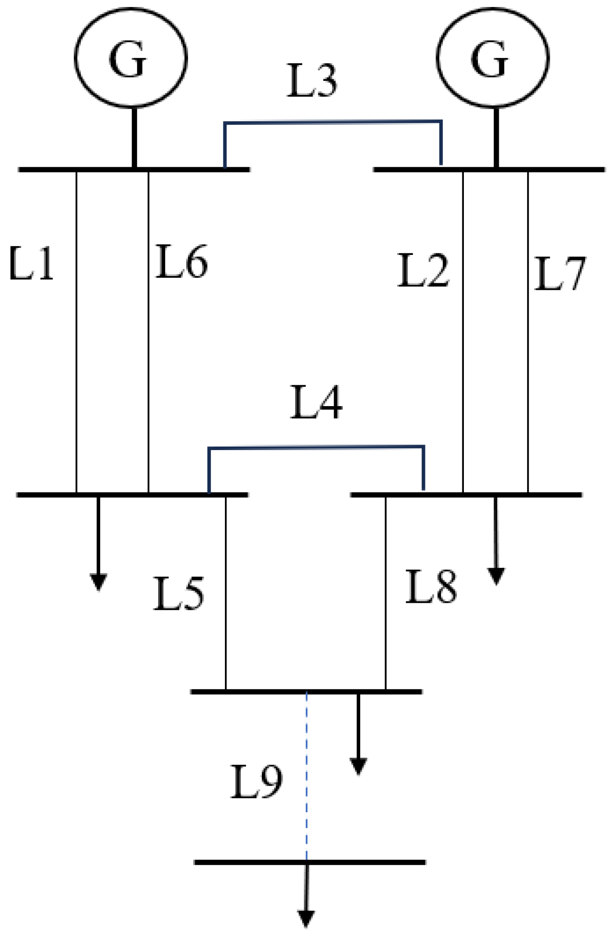
4.2. IEEE RBTS6 Node System

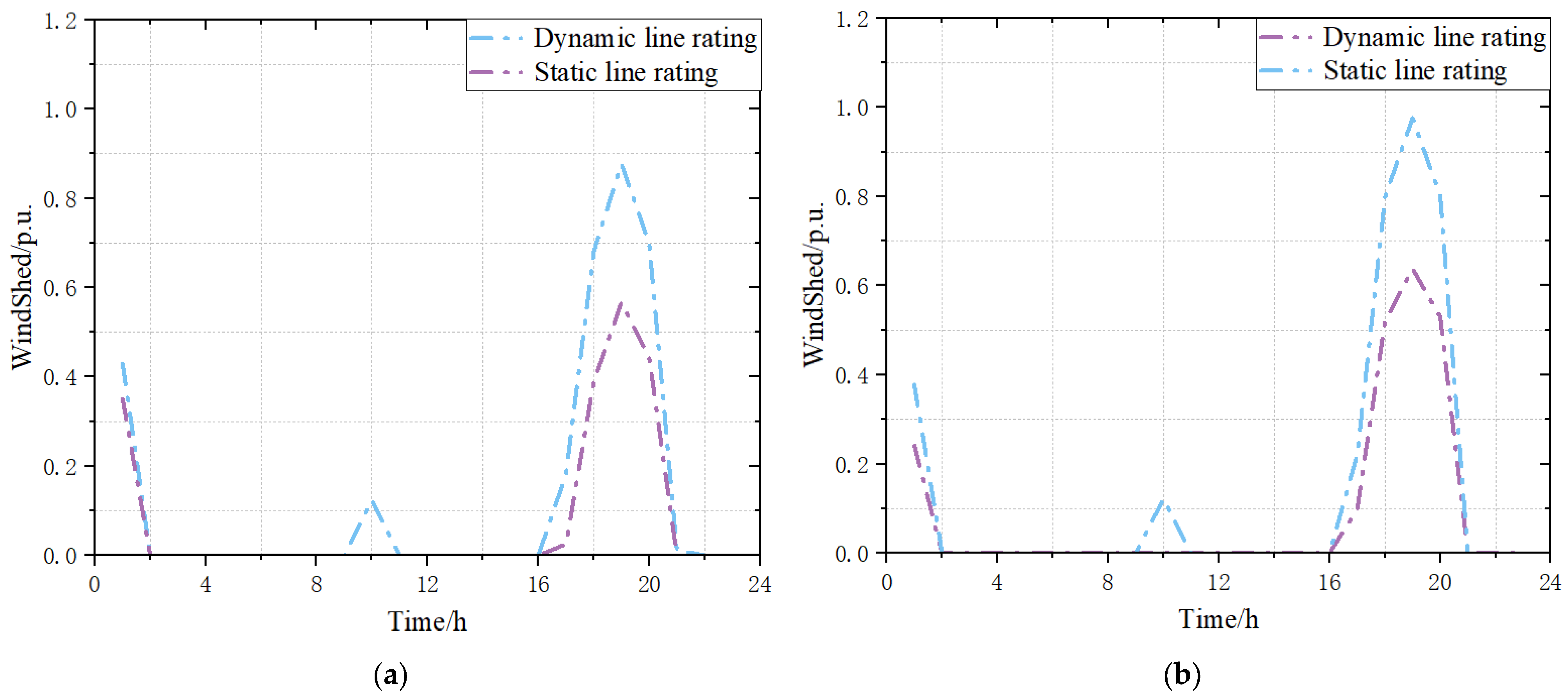
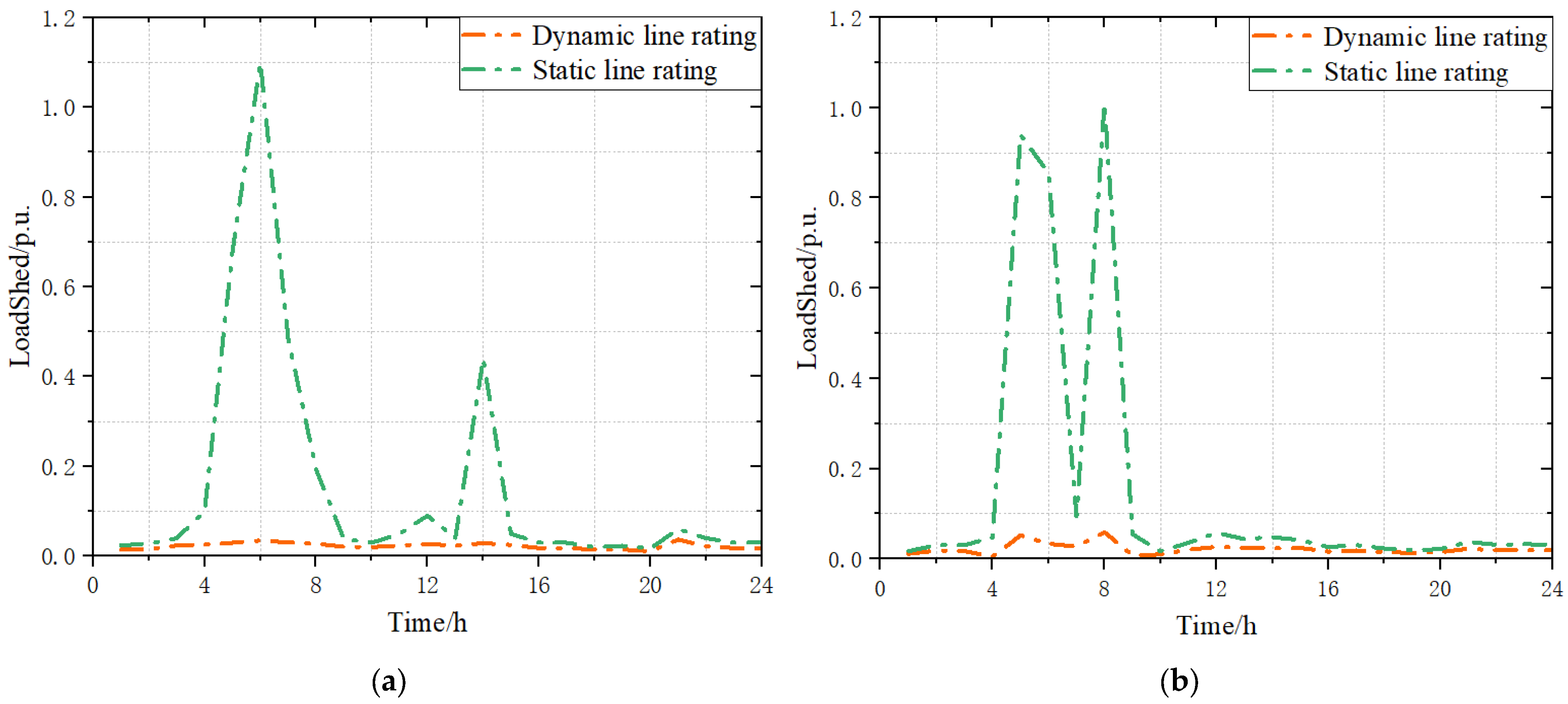
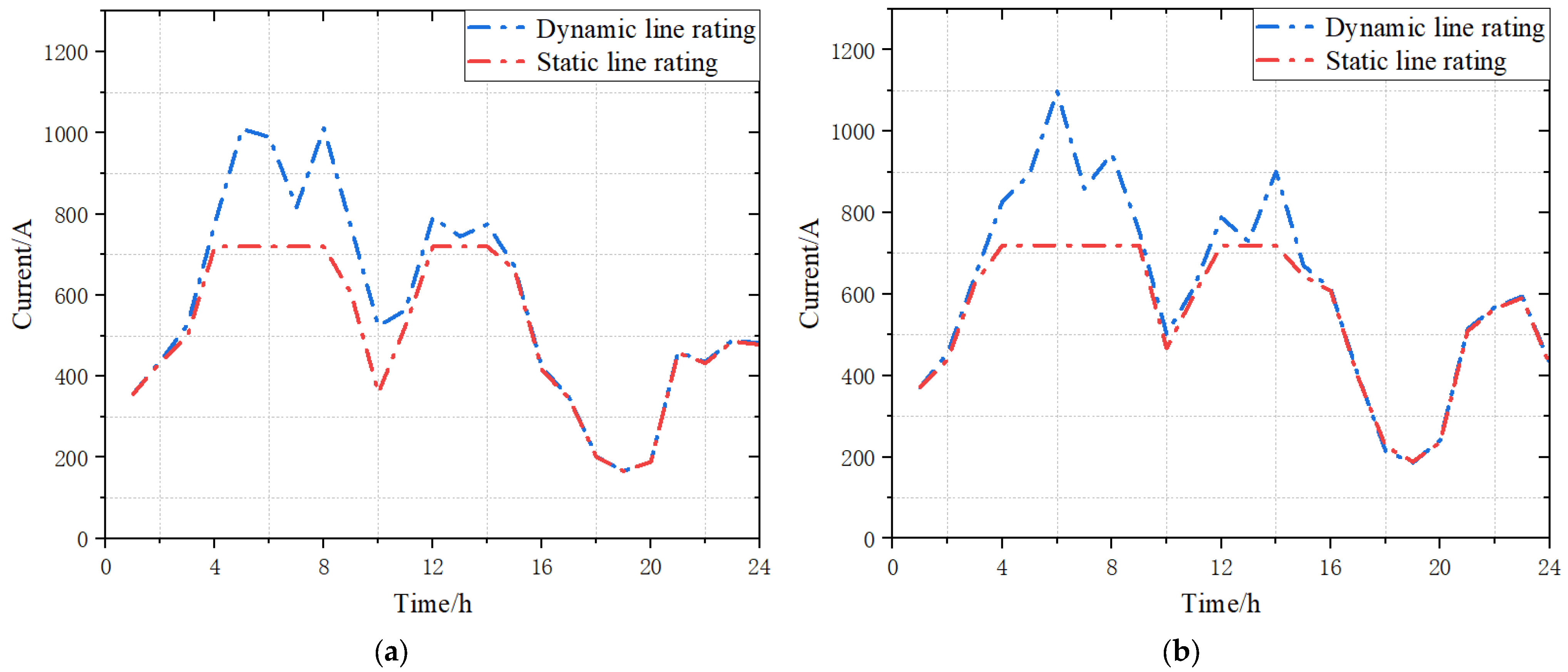
(1)

Effectiveness analysis of the dynamic capacity increase

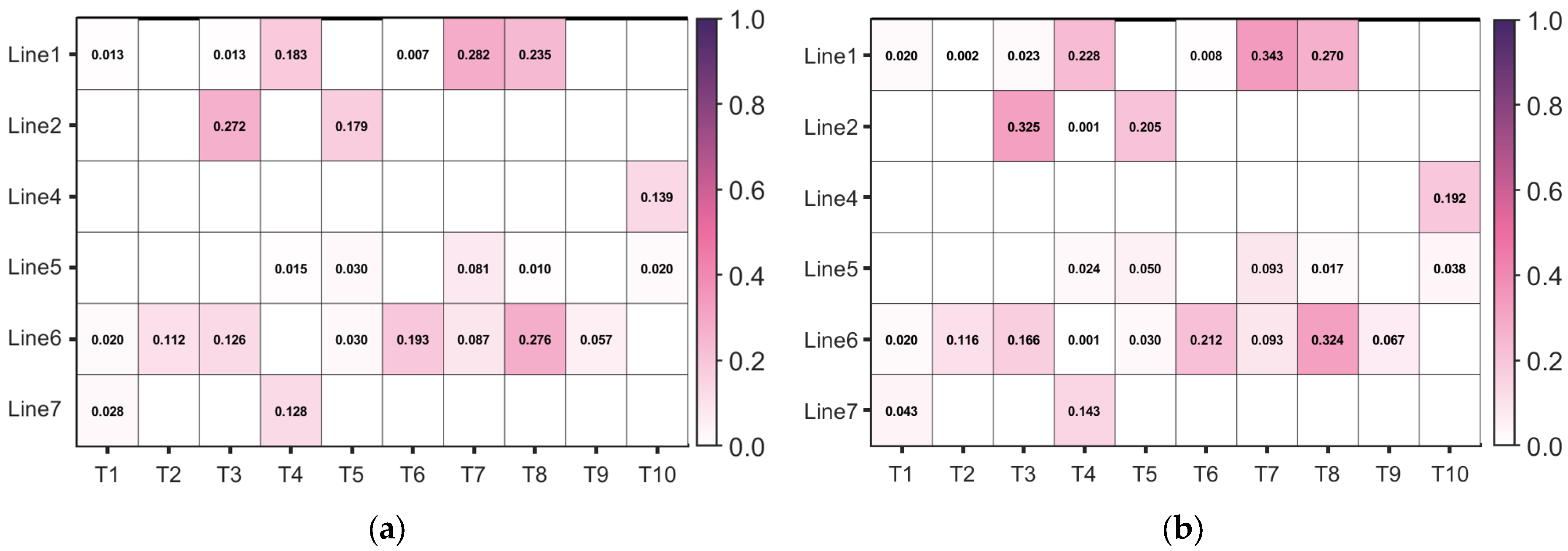
To verify the effectiveness of dynamic line rating technology in alleviating power flow congestion, this section selects two typical scenarios: normal system operation and Line 4 fault conditions. Using the system without DLR as the benchmark, we compare the wind curtailment levels, load shedding levels, and line ampacity capacities before and after implementing DLR technology. The comparative results are illustrated in Figure 4, Figure 5 and Figure 6.

The comparative data from two typical scenarios demonstrate that dynamic line rating technology significantly enhances the utilization of the transmission capacity. During peak electricity demand periods, lines employing the dynamic line rating achieved maximum ampacity values of 1011A and 1098A; these values represent improvements of 39.1% and 51.0%, respectively, with respect to the conservative static line rating of 727A. During high wind power generation periods, the increased transmission capacity enabled by the dynamic line rating reduced wind curtailment by 41.9% and 40.8%; this allowed the system to integrate more renewable energy. In high-load scenarios, the expanded transmission capacity through the dynamic line rating decreased the load shedding requirements by 86.8% and 85.3%; this effectively eliminated the need for large-scale load curtailment measures.

(2)

Analysis of overload risk assessment results considering the influence of component failure

However, when dynamic capacity expansion technology is used, if the line capacity is overestimated, the system may face an overload risk; this could lead to potential faults or even chain reactions. In this section, a risk assessment framework is constructed for the application scenario of ultrashort-term prediction by using the rolling time window analysis method. To analyze the dominant causes of overload risk, a 15-min time step is set within each time window for a continuous 4-h period, and a total of 16 time periods is analyzed.

Based on the intensity and duration of the overload probability occurrence, 10 typical high-risk time periods are selected. The expected overload probability results for transmission lines under multiple scenarios are shown in Figure 7.

A comparison of the results from overload risk case analysis with and without considering component failure reveals that incorporating component failure increases the average overload probability during 10 typical high-risk periods from 0.043 to 0.051. The peak overload probability risks for the different transmission lines also increase to varying degrees. Among these, Line 4 is the most sensitive to component failures. After considering component failures, the peak overload probability for Line 4 increases from 0.139 to 0.192; this represents an increase of 38.1%. The sensitivity of Line 4 indicates that component failures can intensify the overload risks through the vulnerable lines in the network topology. Thus, these results highlight the importance of accounting for component reliability in risk assessments.

Furthermore, the case study results reveal that Line 6 has the highest risk concentration, followed by Line 1 and Line 2, whereas Lines 7 and 5 have relatively fewer high-risk scenarios. The peak overload probability risk for Line 1, which has a higher baseline overload probability level, increases from 0.282 to 0.343; this represents an increase of 21.6%. Similarly, the peak risk for Line 2 increases from 0.275 to 0.325; this represents an increase of 18.2%. For Line 6, the peak risk increases from 0.276 to 0.324; this represents an increase of 17%. Thus, the primary cause of higher overload levels is the significant power transmission burden on these lines during specific periods, along with the influence of environmental parameters; additionally, our results highlight the substantial amplifying effect of the component failures on the system risk. These findings emphasize the critical need to incorporate component failure scenarios in risk assessments to accurately capture and mitigate potential overload risks in power systems.

4.3. IEEE-RTS79 System

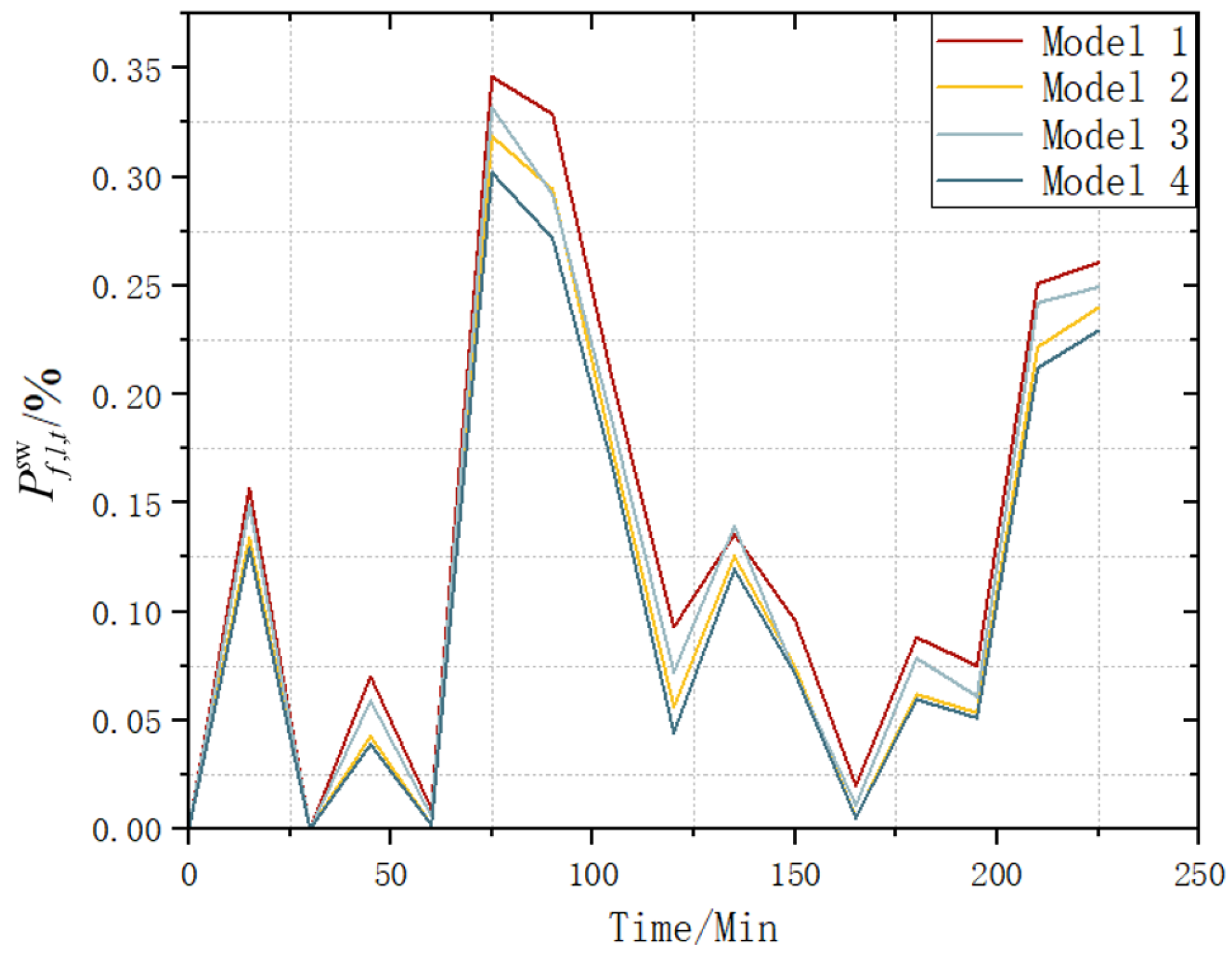
(1)

Influence of the different methods for the determination of the efficiency and accuracy

To evaluate the computational efficiency and accuracy of the proposed transmission line overload risk assessment method, tests were conducted using the IEEE-RTS79 system. Four distinct overload risk assessment models were implemented:

Model 1: DLR is used, and the risk is assessed using the first-order reliability method (FORM).

Model 2: DLR is used, and the overload probability is evaluated using the second-order reliability method (SORM), as proposed in this study.

Model 3: DLR is incorporated, and the overload probability is estimated using the multipoint estimate method (MPEM) [31].

Model 4: DLR is incorporated, and the overload probability is estimated using the Monte Carlo method.

A comparative analysis of the probability density functions (PDFs) of expected overload probability obtained from these methods was performed. Figure 8 shows the expected overload probability results for Line 27 in the IEEE-RBTS79 system.

The overall accuracy of the calculation results of Model 1 is good, but the stability is relatively low, as evidenced by a slightly large deviation at the highest point of the probability density. This occurs because it cannot capture the nonlinear changes of some scenarios, thus failing to meet the needs of actual power grid operation. In contrast, the overall accuracy and stability of Model 2 proposed in this paper are greatly improved under the dynamic capacity scenario, achieving the closest approximation effect. Model 3 (MPEM) exhibits moderate accuracy due to its reliance on limited sampling points, which cannot fully resolve higher-order nonlinear effects in DLR-enabled systems.

Real-world power systems demand high-risk assessment accuracy and minimization of the computational overhead; due to these operational requirements, the efficiency of the evaluation method is equally critical.

Table 3. Computational time comparison.

	Model 1	Model 2	Model 3	Model 4
Calculation time (s)	14.8	39.6	77.9	1094.7

provides a comparison of the computation times of the three methods, and the differences in computational efficiency are quantified.

As evident from the results, the proposed SORM-based method (Model 2) significantly reduces the computation time with respect to the Monte Carlo method (Model 4) and provides an efficient and accurate solution for overload risk assessment in DLR-enabled scenarios. While Model 3 (MPEM) improves upon Model 4 in speed, it requires significantly more computation time than Model 2 due to repeated function evaluations in nonlinear scenarios and is less accurate in nonlinear cases.

5. Conclusions

DLR technology significantly enhances the grid’s ability to integrate renewable energy and simultaneously embeds the transmission capacity uncertainties deeply into system operations. An integrated overload risk assessment framework that incorporates multiple uncertainties is proposed. First, the second-order reliability method (SORM) is utilized to efficiently characterize the continuous stochasticity of environmental parameters using analytical approximations. Second, a multiscenario stochastic analysis model is established; this model unifies the equipment failures, load fluctuations, and dynamic capacity contraction within a single assessment framework and enables the accurate risk evaluation under complex operating conditions. The case study results demonstrate that the proposed method achieves comparable accuracy to that of the Monte Carlo method and significantly improves the computational efficiency; thus, this method is highly practical for large-scale power system risk assessments.

The focus of this study is on transmission line overload risk assessment; thus, future research will extend the framework to incorporate risk mitigation and dynamic corrective measures. Key directions include integrating time-dependent couplings of energy storage response and topology reconfiguration into the model and exploring coordinated optimization strategies for DLR-enabled systems under extreme weather events.

Additionally, while the modified IEEE test systems (e.g., IEEE-RTBS 6-node and IEEE-RTS79) capture essential dynamics such as renewable integration and N-1/N-2 contingencies, they simplify certain complexities inherent to real-world large-scale power networks. For instance, interactions between voltage stability, frequency regulation, and cascading failures are not fully emulated. Finally, interdependencies among geographically distributed components (e.g., correlated wind farms) may require further modeling refinements. Future work will extend this framework to realistic grids using decomposition techniques (e.g., network partitioning) and high-performance computing to address scalability.

References

1. Yu, Z.; Liu, X.; Yan, K.; Song, Y.; Zhou, K. Combination Model of Chance-constrained Security Constraint Unit with Considering the Forecast Uncertainties of DLR and Wind Power. High Volt. Eng. 2021, 47, 1204–1214. [Google Scholar] [CrossRef]
2. IEEE Std 738-2006 (Revision of IEEE Std 738-1993); IEEE Standard for Calculating the Current-Temperature of Bare Overhead Conductors. IEEE Standard Association: Piscataway, NJ, USA, 2007; pp. 1–58. [CrossRef]
3. Karimi, S.; Musilek, P.; Knight, A.M. Dynamic thermal rating of transmission lines: A review. Renew. Sustain. Energy Rev. 2018, 91, 600–612. [Google Scholar] [CrossRef]
4. Peng, X.; Peng, R.; Wang, R.; Guo, D.; Fan, Y.; Liu, G. Equivalent Heat Transfer Transient Measurement Model for Dynamic Capacity Increase of Overhead Transmission Lines. High Volt. Technol. 2022, 48, 3975–3986. [Google Scholar]
5. Wang, T.; Zhu, S.; Guo, R.; Qu, X. Study on the dynamic current carrying capacity of the parallel grid line of Baihubao wind farm in Pinglu Shanxi province. Power Syst. Technol. 2016, 40, 1400–1405. [Google Scholar]
6. Hou, Y.; Wang, W.; Wei, Z.; Deng, X.; Ji, Q.; Wang, T.; Ru, X. Research and application of dynamic line rating technology. Energy Rep. 2020, 6, 716–730. [Google Scholar] [CrossRef]
7. Lawal, O.A.; Teh, J. Assessment of dynamic line rating forecasting methods. Electr. Power Syst. Res. 2022, 214, 108807. [Google Scholar] [CrossRef]
8. Viafora, N.; Morozovska, K.; Kazmi, S.H.H.; Laneryd, T.; Hilber, P.; Holbøll, J. Day-ahead dispatch optimization with dynamic thermal rating of transformers and overhead lines. Electr. Power Syst. Res. 2019, 171, 194–208. [Google Scholar] [CrossRef]
9. Gao, Z.; Hu, S.; Jin, T.; Sun, H.; Chen, X.; Wang, Z. Day-ahead power system scheduling model considering transmission line dynamic capacity expansion risk. High Volt. Eng. 2023, 49, 3215–3226. [Google Scholar]
10. Wallnerstrm, C.J.; Huang, Y.; Sder, L. Impact from Dynamic Line Rating on Wind Power Integration; IEEE Press: New York, NY, USA, 2015. [Google Scholar] [CrossRef]
11. Wang, K.; Sheng, G.; Sun, X.; Wang, W.; Wang, S.; Jiang, X. Online prediction of transmission dynamic line rating based on radial basis function neural network. Dianwang Jishu/Power Syst. Technol. 2013, 37, 1719–1725. [Google Scholar] [CrossRef]
12. Zhu, X.; Xue, Y.; Huang, T. Complexity of Influence of Generator Inertia on Transient Angle Stability. Autom. Electr. Power Syst. 2019, 43, 102–108. [Google Scholar]
13. Wang, C.; Liu, F.; Wang, J.; Wei, W.; Mei, S. Risk-Based Admissibility Assessment of Wind Generation Integrated into a Bulk Power System. IEEE Trans. Sustain. Energy 2015, 7, 325–336. [Google Scholar] [CrossRef]
14. Ding, Z.; Yu, K.; Wang, C.; Lee, W.J. Transmission Line Overload Risk Assessment Considering Dynamic Line Rating Mechanism in a High-Wind-Penetrated Power System: A Data-Driven Approach. IEEE Trans. Sustain. Energy 2022, 13, 1112–1122. [Google Scholar] [CrossRef]
15. Zhaohao, D.; Kaiyuan, Y.; Cheng, W. Overload Risk Assessment of Power Transmission Line Considering Dynamic Line Rating. Autom. Electr. Power Syst. 2021, 45, 146–152. [Google Scholar]
16. Cai, X.; Dang, P.; Zeng, W. Application Status and Development Trend of Capacity-Increase Technology for Overhead Transmission. Wire Cable 2023, 66, 1–6. [Google Scholar] [CrossRef]
17. Xingang, Y.; Yanxue, Z.; Yajun, Z. Improved method for improving iterative convergence of short circuit calculation in new energy AC power grid. Electr. Power Autom. Equip. 2024, 44, 185192–185209. [Google Scholar] [CrossRef]
18. Ma, Y.; Liu, C.; Xie, K.; Hu, B.; Yang, H. Review on Network Transmission Flexibility of Power System and Its Evaluation. CSEE 2023, 43, 5429–5441. [Google Scholar]
19. Aznarte, J.L.; Siebert, N. Dynamic Line Rating Using Numerical Weather Predictions and Machine Learning: A Case Study. IEEE Trans. Power Deliv. 2017, 32, 335–343. [Google Scholar] [CrossRef]
20. Guang, M.; Yining, Z.; Zhe, C. Risk assessment method for hybrid AC/DC system with large-scale wind power Integration. Power Syst. Technol. 2019, 43, 3241–3252. [Google Scholar] [CrossRef]
21. Ye, K.; Zhao, J.; Hong, M.; Maslennikov, S.; Tan, B.; Luo, X. Power System Overloading Risk Assessment Considering Topology and Renewable Uncertainties. In Proceedings of the 2024 IEEE Power & Energy Society General Meeting (PESGM), Seattle, WA, USA, 21–25 July 2024; pp. 1–5. [Google Scholar]
22. Matus, M.; Saez, D.; Favley, M.; Suazo-Martinez, C.; Moya, J.; Jimenez-Estevez, G.; Palma-Behnke, R.; Olguin, G.; Jorquera, P. Identification of Critical Spans for Monitoring Systems in Dynamic Thermal Rating. IEEE Trans. Power Deliv. 2012, 27, 1002–1009. [Google Scholar] [CrossRef]
23. Breitung, K. Asymptotic approximations for multinormal integrals. J. Eng. Mech. ASCE 1984, 110, 357–366. [Google Scholar] [CrossRef]
24. Fu, S. Research on Probability Prediction Method of Carrying Capacity of Overhead Conductor. Master’s Thesis, Shandong University, Jinan, China, 2019. [Google Scholar]
25. Chen, P.; Pedersen, T.; Bak-Jensen, B.; Chen, Z. ARIMA-Based Time Series Model of Stochastic Wind Power Generation. IEEE Trans. Power Syst. 2010, 25, 667–676. [Google Scholar] [CrossRef]
26. Liu, Y.; Li, W.; Liu, C. Mixed skew distribution model for short-term wind power prediction error. Proc. CSEE 2015, 35, 2375–2382. [Google Scholar]
27. Zhao, S.; Shao, C.; Ding, J.; Hu, B.; Xie, K.; Yu, X.; Zhu, Z. Unreliability Tracing of Power Systems for Identifying the Most Critical Risk Factors Considering Mixed Uncertainties in Wind Power Output. In Protection and Control of Modern Power Systems; IEEE: Piscataway, NJ, USA, 2024; Volume 9, pp. 96–111. [Google Scholar] [CrossRef]
28. Long, X. A Fully Analytical Approach for the Real-Time Dynamic Reliability Evaluation of Composite Power Systems with Renewable Energy Sources. Engineering 2024, in press. [Google Scholar] [CrossRef]
29. Yang, W.; Cao, M.; Ge, P.; Hu, B.; Qu, G.; Xie, K.; Cheng, X.; Peng, L.; Yan, J.; Li, Y. Risk-Oriented Renewable Energy Scenario Clustering for Power System Reliability Assessment and Tracing. IEEE Access 2020, 8, 183995–184003. [Google Scholar] [CrossRef]
30. Wang, T. Research on Short-Term Current-Carrying Capacity Prediction Method of Overhead Conductor; Shandong University: Jinan, China, 2022. [Google Scholar]
31. Han, H.; Gao, S.; Dai, J.; Chen, Y. A new multi-point estimate method on uncertain power flow. In Proceedings of the 2014 International Conference on Power System Technology, Chengdu, China, 20–22 October 2014; pp. 440–444. [Google Scholar]
Figure 1. SORM method diagram.
Energies 18 01822 g001
Figure 2. System state generation process.
Energies 18 01822 g002
Figure 3. Improved IEEE-RTBS 6-node test system.
Energies 18 01822 g003
Figure 4. Comparison of wind curtailment levels under normal operation and Line 4 fault scenarios. (a) Wind curtailment level under normal operation scenario; (b) wind curtailment level under Line 4 fault conditions.
Energies 18 01822 g004
Figure 5. Comparison of load shedding levels under normal operation and Line 4 fault scenarios. (a) Load shedding level under normal operation scenario; (b) load shedding level under Line 4 fault scenario.
Energies 18 01822 g005
Figure 6. Comparison of line loadability levels under normal operation and Line 4 fault scenarios. (a) Line loadability level under normal operation scenario; (b) line loadability level under Line 4 fault scenario.
Energies 18 01822 g006
Figure 7. Overload risk analysis of the transmission lines. (a) Without component failure; (b) considering component failure.
Energies 18 01822 g007
Figure 8. Overload risk analysis considering the component failures.
Energies 18 01822 g008