Applicability of a Heat Recovery Ventilator Retrofit in a Vancouver Residential House

Abstract

Heat recovery systems are increasingly recognized as key energy conservation measures in residential buildings. But their effectiveness is highly sensitive to operational conditions. This study used a calibrated OpenStudio simulation, which is validated against monthly utility data, to investigate the feasibility of implementing a heat recovery ventilator in an existing single-detached house in Vancouver under two scenarios: existing passive ventilation without a heat recovery ventilator versus the proposed balanced mechanical ventilation with a heat recovery ventilator. The findings indicate that employing an HRV in an existing house lacking balanced ventilation would lead to higher annual space heating energy consumption (75.49 GJ electricity and 56.70 GJ natural gas with HRV compared to 73.64 GJ and 52.70 GJ, respectively, without an HRV). Therefore, for existing houses without balanced ventilation, improving the existing building envelope’s airtightness through retrofits should always be carried out before installing a heat recovery ventilator. Additionally, the heat recovery ventilator should be appropriately sized to compensate for any shortfall in natural infiltration to ensure the sufficient indoor air quality while minimizing the outdoor air-induced space heating energy usage. Furthermore, the recommended break-even point of the infiltration rate for the house studied in this work to avoid increased space heating energy use due to the retrofit with a heat recovery ventilator is 0.281 air change per hour.

1. Introduction

Energy is essential to all aspects of modern life; however, excessive energy use is a major contributor to greenhouse gas (GHG) emissions, which drive global warming. To limit global warming and prevent the earth temperature from rising by more than 2 °C above pre-industrial levels, one hundred ninety-six (196) parties, including Canada, adopted the Paris Agreement—an international treaty on climate change from 2015. This agreement aims to achieve global climate neutrality by 2050 [1]. To contribute to this global target, Canada has put forth a climate plan and committed to achieving net-zero emissions nationwide by 2050 [2]. Undoubtedly, integrating the sustainable development principles and employing applicable energy conservation measures across all Canadian economic sectors, including the building sector, would make the national GHG mitigation target more attainable. In Canada, the building sector contributes 13% of the national GHG emissions, making it the third largest emitter in the country [3]. Within this sector, single-detached homes represent the most common dwelling type and a major source of energy consumption. In 2016, approximately 69% of the nation’s energy was attributed to single-detached homes [4]. Therefore, improving the energy efficiency of these homes is crucial for reducing Canada’s overall emissions.

Canada is a heating-dominant country. According to Natural Resources Canada, space heating accounts for 67% of secondary energy use in residential single-detached homes [5]. Extensive research has been conducted to evaluate the various energy conservation measures (ECMs) and their effectiveness in reducing space heating energy consumption. In general, these ECMs can be categorized into two main approaches: (1) improving the performance of the buildings’ mechanical, electrical and plumbing (MEP) systems, and (2) reducing the buildings’ thermal demand. The first approach involves integrating high-efficiency MEP systems into building designs [6,7], for example, by utilizing the heat pump (HP) technology to increase the thermal efficiency of space heating and domestic hot water systems [8], or by employing variable frequency drives (VFDs) to optimize pump and fan energy consumption under part-load conditions [9]. The second approach focuses on reducing the buildings’ thermal demand by enhancing the thermal performance of building enclosures, such as increasing envelope insulation levels and improving airtightness to minimize uncontrolled air leakage between the buildings’ exterior and interior [6,10,11,12].

Reducing the thermal demand allows for smaller-sized heating equipment, thereby reducing the space heating energy consumption. As a key contributor to the buildings’ heating loads, ventilation plays an important role in reducing the buildings’ thermal demand. Approximately 18–35% of the energy delivered to residential buildings is used for conditioning ventilation air [6,13]. Ventilation is a process of replacing staled indoor air with fresh outside air to maintain an acceptable indoor air quality. However, to minimize indoor thermal discomfort, this fresh air must be conditioned before entering the living space; therefore, the ventilation-induced heat loss must be accounted for in the building’s heating load calculations to ensure the proper sizing of the space heating equipment, such as boilers or furnaces. With the growing awareness of sustainable practices in the building sector, residential buildings are increasingly designed with a high performance enclosure featuring an improved thermal resistance and lower infiltration rates. While this significantly reduces the building’s heating demand by minimizing conductive and infiltration- related heat losses, it also makes ventilation-induced heat loss more pronounced. This is because tightly sealed buildings have much less infiltration. To maintain an acceptable indoor air quality, mechanical ventilation systems with properly designed airflow are needed. Reducing ventilation-induced heating loads not only lowers the overall building thermal demand but also allows for the use of smaller heating equipment and reduces the space heating energy consumption.

As a proven energy conservation measure, heat recovery ventilators (HRVs), and energy recovery ventilators (ERVs) have been highly recommended by various building codes and/or energy standards, such as the BC Building Code (BCBC) and Passive House Institute, and are mandated in the Vancouver Building By-Law (VBBL). These systems help mitigate the ventilation-induced heat loss by recovering heat from the outgoing exhaust air and transferring it to the incoming fresh air, thereby reducing the temperature difference between the two air streams. Numerous studies have demonstrated that although HRVs/ERVs can effectively lower a building’s thermal demand and reduce space heating energy use, their performance is influenced by several factors, including outdoor climatic conditions [14,15,16,17,18]; building mechanical system type [16,19,20]; ventilation air flowrate [14,19,21]; indoor cooling and heating temperature setpoints [22,23]; building operation schedules [24]; and building envelope tightness [20,23,25].

For new construction buildings, potential negative interactive effects between the afore-mentioned factors and HRV/ERV energy performance can be minimized by adjusting the relevant design parameters of the building’s energy systems during the design stage. However, for existing buildings, many of these parameters are fixed since the building has already been constructed and occupied. Making changes to the existing, in-place energy systems, such as envelope systems, space heating equipment, and distribution systems, to optimize the HRV/ERV performance could be costly and challenging. In Canada, many existing single-family detached homes are ventilated by the exhaust-only ventilation systems (i.e., passive ventilation), which use the exhaust air fans to exhaust the indoor stale air to the outside. However, HRVs/ERVs require a balanced ventilation setup. This discrepancy means that the existing exhaust-only ventilation systems would need to be replaced with balanced ventilation systems to accommodate the HRVs/ERVs. Furthermore, comprehensive examinations of interactive effects between HRVs and other existing building energy systems are rarely addressed in government-issued building codes or industry design standards. Given that single-detached homes dominate the existing building stock in Canada [26], optimizing ventilation-induced thermal demand by appropriately integrating HRV/ERV technologies with the building’s existing energy systems is crucial for achieving the national GHG mitigation targets.

2. Background

A number of studies have investigated the energy-saving effectiveness of employing HRVs in a building’s HVAC systems. For example, Li et al. [18] investigated the impact of a building’s orientations and outdoor climatic conditions on the heating energy use reductions due to the HRV use in a typical Canadian apartment suite. In their study, a series of TRNSYS models were developed to simulate the energy use of an air-to-air heat pump system serving a hypothetical apartment suite, facing different azimuth angles, and located in fifteen Canadian cities across three climate zones. Zhou et al. [22] explored the impacts of an indoor setpoint on an ERV’s energy saving performance through a series of EnergyPlus simulations. In their study, the ERV was coupled with decentralized air-conditioning systems serving office buildings located in two cities with distinct climates in China. Liu et al. [14] conducted a simulation-based study on the energy-saving performance of an ERV coupled with floor-radiant heating systems in a residential apartment building in China during the heating season (October to March). Although these simulation-based studies enabled the researchers to scrutinize the applicability of incorporating HRVs or ERVs into various HVAC systems under different conditions without setting up real-world systems, there often exists a significant discrepancy in results between model predictions and actual measurements. This mismatch can be attributed to factors such as differences in occupancy, lighting, miscellaneous load, and temperature schedules, the energy performance characteristics of heating and cooling devices, control sequences, envelope thermal properties and tightness, and weather conditions between the simulation and reality [27,28].

A measurement, on the other hand, allows the researchers to assess the HRV’s energy performance based on the measured parameters such as the flowrates, temperatures, moisture content, and electric power consumption of both exhaust and supply fans of the HRV. These key parameters are often measured under controlled laboratory conditions which may not necessarily reflect real-life operating conditions; therefore, results of such studies might not accurately represent the system’s runtime energy performance. For example, Delfani et al. [29] conducted an experimental study to examine the impacts of four different installation and configuration strategies for coupling an HRV with an air-conditioning system to achieve reductions in cooling coil load. In their study, forty different thermal statuses of the air were created by a lab experimental facility to represent the HRV’s outside air intake under various outdoor climatic conditions. The flowrate of the airstream in all the testing cases was controlled at 680 m³/hr, while the temperatures of the cooling coil outlet air, space supply and return airstream remained constant. The mixing ratio of outside air and return air was also held constant across all tests. However, since the study was conducted under controlled laboratory conditions, it did not report the influence of variations in cooling coil supply and return air temperatures, which often occur under real-life conditions. In a similar vein, Idayu et al. [30] investigated the performance of an ERV under various operating conditions through an experimental setup in a small-scale experimental test room constructed of plywood. The room was heated with an artificial heater inside the space and ventilated by an energy recovery unit placed on top. The heat recovery performance of the ERV was calculated based on the measured temperatures, moisture content, and flow rates of the supply and exhaust airstreams in the ERV under various air velocities. Although, the conclusions of the study offer insights into the trends of energy exchange effectiveness of the ERVs operating under other different ranges of air velocity, they are specific to the controlled laboratory conditions in the study, including the supply air intake temperature, airstream velocity, ductwork size, configuration and materials of the ERV energy exchange core, and chamber indoor temperature. Similarly, Pekdogan et al. [31] conducted an experimental study at the Building Physics laboratory of Izmir Institute of Technology to investigate the optimized switching period of the ventilation modes for a wall-mounted ceramic thermal storage type HRV. Key parameters, such as velocities and temperatures of the airstreams inside the duct and ceramic heat exchange core, were measured. The switching periods for ventilation modes were tested at 1, 2, 5, 7.5, and 10 min, with results showing the best heat transfer performance when the switching period was set to 2 min. Again, the results are specific to the laboratory testing conditions. Other measurement-based HRV performance studies can be found in [32,33,34].

The simulation calibration method strikes a balance between the two approaches. It involves three major steps: pre-retrofit building energy modeling, model calibration, and post-retrofit building performance simulation based on the calibrated energy model. This method allows for the simulation of energy savings from various ECMs under different operation conditions. During the literature review, several studies using this method were identified; however, most focused on quantifying the overall building energy reductions resulting from the implementation of multiple ECMs (ECM bundle) applied together to a building. The specific contribution of an HRV to the overall energy savings was not explicitly addressed. For example, Jermyn et al. [35] investigated the impacts of deep energy retrofits to both envelope and HVAC systems on energy use in three styles of existing homes (century home, century-semi home, and war time home) in Toronto by performing a series of building energy simulations. The building envelope retrofits included envelope thermal performance improvement while HVAC system retrofits focused on adding the heat recovery ventilator and enhancing the efficiency of heating and cooling equipment. The study adopted Brute Force Sequential Search methodology to identify and iteratively optimize the retrofit strategies for achieving the best balance between energy savings and retrofit costs. However, the specific contribution of the HRV to energy savings is not addressed explicitly. Fleur et al. [36] studied energy use in a typical apartment suite before and after a retrofit in Sweden. The building was modeled in IDA ICE based on the field measurements and building plans to simulate energy use, space heating loads, and indoor climate, respectively. The envelope renovation included adding insulation to the entire envelope and replace windows with well-insulated ones. The existing exhaust-only ventilation system was replaced with a balanced ventilation system coupled with an HRV. Although the results of the study reported a significant reduction in building energy use after the retrofit, the contribution of the HRV to these savings was not explicitly discussed.

Upon reviewing the literature, it is evident that although the energy saving performance of HRVs has been extensively studied through theoretical simulations and experimental measurements, these studies often face challenges such as discrepancies between models and real-world scenarios, or limitations in generalizability. The simulation calibration method, which combines the advantages of both simulation-based and experiment approaches, allows us to bridge this gap. However, its application in evaluating the specific contribution of HRVs to overall building energy performance remains limited.

Therefore, the overarching objective of the study is to examine the applicability of incorporating an HRV into an existing gas-fired furnace heating system in a single-family house in Vancouver’s climate zone with a particular focus on the interactive effects between the HRV and the airtightness of the house’s existing envelopes. To achieve this, an OpenStudio energy model of the house was developed and calibrated to accurately reflect its current energy performance. Consequently, simulations were conducted to compare the annual space heating energy consumption of the system with and without HRV. The following section (Section 2) details the research methodology encompassing the introduction of simulation tools used in the study, description of the existing residential dwelling house along with its host mechanical systems, modeling process, and key metrics evaluated in the study. Finally, the analysis based on the calibration model and the corresponding conclusions are presented in Section 3 and Section 4, respectively, followed by the limitations and suggestions for future research directions in Section 5.

3. Methodology

In the study, a 3D SketchUp model of the house was developed based on its as-built architectural drawings provided by the owner. The building design and construction details such as geometry, space utilization, construction materials, and energy-influencing systems were verified through an on-site walkthrough. Additionally, an interview was conducted to have a better understanding of the occupant’s lifestyle and energy use behaviors. The 3D SketchUp model was then imported into the OpenStudio^® application, where all building energy systems, including envelope assemblies, HVAC and domestic hot water systems, electrical lighting, and other miscellaneous appliances were modeled. To ensure the energy model accurately reflected the building’s real-life thermal behavior and energy performance characteristics, it was calibrated by replacing the typical meteorological year (TMY) weather file with the actual weather data and adjusting the selected input values accordingly. The applicability of employing an HRV was then examined by comparing the simulated space heating energy use of the system with and without the HRV, based on the calibrated model.

3.1. Building Energy Model Description

3.1.1. Simulation Tool

In this study, OpenStudio^®, an open-source building energy simulation software development kit (SDK) developed by the National Renewable Energy Laboratory (NREL), was utilized to develop the building energy model. OpenStudio^® integrates various simulation tools, including EnergyPlus and Radiance, to facilitate comprehensive whole-building energy analysis. Additionally, OpenStudio^® offers a Sketchup plugin, enabling users to create and edit 3D geometry for EnergyPlus models within the Sketchup environment. This integration allows for a seamless workflow in modeling building energy performance from 3D geometry creation to simulation execution [37].

3.1.2. Climate Data

In the study, the single-family house is located in Vancouver. The EPW format weather file representing Vancouver’s typical meteorological year weather was utilized in the initial run of the OpenStudio^® model. The EPW format is developed by the United States Department of Energy (DoE) as a standard weather format. It consolidates annual measured weather data to reflect both local average and extreme weather [38].

3.1.3. Building Description

The building examined in this study is a two-story, wood-framed, single-detached house located in Vancouver, encompassing a total floor area of 289 m². It comprises two sections, the main residence and an attached garage rental suite, as depicted in Figure 1. The main residence has a height of 7.53 m, while the garage rental suite is 6.10 m tall. Figure 2 and Figure 3 illustrate the architectural layouts of the building’s ground and second floors, respectively. As shown in the figures, the ground floor of the main residence includes an open area encompassing the kitchen, dining room, and great room areas; a den; a bathroom; a foyer; and a laundry room. The ground floor of the garage rental suite consists solely of one room (i.e., double garage). The second floor of the main residence houses three bedrooms (master suite, bedroom 2, and bedroom 3); a walk-in closet; and a bathroom. The second floor of the garage rental suite part features a single room referred to as the bonus room.

In the study, each room within the building was set up as a separate thermal zone in the 3D SketchUp model. This approach facilitates the simulation of conductive heat transfer through partition walls, accounting for potential temperature differences between adjacent spaces during the simulation period. The detailed 3D SketchUp model was then exported to the OpenStudio^® application, where additional parameters influencing the building’s thermal behavior were defined, including the construction and thermal properties of the building’s envelope systems, the envelope infiltration rates, and space internal loads.

3.1.4. Envelope Assemblies Model

The construction and thermal properties of the building envelope were modeled based on the as-built drawings provided by the homeowner. The exterior walls were represented as 50 mm × 150 mm (2 × 6) wood-framed walls with studs spaced 400 mm apart, with a cavity insulation with an RSI value of 3.52. The roof above the conditioned space was modeled as a 50 mm × 300 mm wood joist roof with RSI-4.93 batt insulation between the joists. The ceiling above the conditioned space was modeled as a 15.88 mm gypsum board with RSI-7.04 continuous batt insulation installed on the attic side. The second floor was modeled with 50 mm × 250 mm wood floor joists without insulation. Detailed layers and thermal properties of these envelope components are summarized in

Table 1. Envelope construction and thermal properties.

Envelope Assemblies	Assembly Layers (from Outside to Inside)	U-Factor ($\mathbf{w}/{\mathbf{m}}^2·\mathbf{K}$)
Roof	Cedar sharks Building paper 50.8 mm × 101.6 mm spaced sheathing 50 mm × 300 mm wood roof joist RSI-4.93 batt insulation 6 mil Poly V.B. 15.88 mm gypsum board	0.208
Ceiling	RSI-7.04 batt insulation 6 mil Poly V.B. 15.88 mm gypsum board	0.214
Exterior Wall	Horizontal siding Building paper 9.53 mm poly sheathing 50 mm × 50 mm (2 × 6) wood studs RSI-3.52 batt insulation 6 mil Poly V.B. 12.7 mm gypsum board	0.354
Second Floor	Finish floor 19.05 mmT&G Plywood subfloor 50 mm × 250 mm wood floor joist 50.8 mm × 50.8 mm cross bridging 12.7 mm gypsum board	0.382

.

3.1.5. Infiltration Rate

The building’s infiltration rate input to the model is 6.31 air changes per hour at 50 Pascals (${ACH}_{50}$), which is derived from a blower door test conducted by a third party. According to the Energy Star Home Sealing Specification [39], ${\mathrm{A}\mathrm{C}\mathrm{H}}_{50}$ can be converted to natural air changes per hour (${ACH}_{natural}$) with Equation (1). In the equation, the LBL factor is 17.2, and ${\mathrm{A}\mathrm{C}\mathrm{H}}_{\mathrm{n}\mathrm{a}\mathrm{t}\mathrm{u}\mathrm{r}\mathrm{a}\mathrm{l}}$ is calculated to be 0.367.

$${ACH}_{natural}={\displaystyle \frac{{ACH}_{50}}{LBL factor }}$$

(1)

where

${\mathrm{A}\mathrm{C}\mathrm{H}}_{\mathrm{n}\mathrm{a}\mathrm{t}\mathrm{u}\mathrm{r}\mathrm{a}\mathrm{l}}=\mathrm{A}\mathrm{i}\mathrm{r} \mathrm{c}\mathrm{h}\mathrm{a}\mathrm{n}\mathrm{g}\mathrm{e}\mathrm{s} \mathrm{p}\mathrm{e}\mathrm{r} \mathrm{h}\mathrm{o}\mathrm{u}\mathrm{r} \mathrm{a}\mathrm{t} \mathrm{n}\mathrm{o}\mathrm{r}\mathrm{m}\mathrm{a}\mathrm{l} \mathrm{p}\mathrm{r}\mathrm{e}\mathrm{s}\mathrm{s}\mathrm{u}\mathrm{r}\mathrm{e} \mathrm{d}\mathrm{i}\mathrm{f}\mathrm{f}\mathrm{e}\mathrm{r}\mathrm{e}\mathrm{n}\mathrm{t}\mathrm{i}\mathrm{a}\mathrm{l}$

${\mathrm{A}\mathrm{C}\mathrm{H}}_{50}=\mathrm{A}\mathrm{i}\mathrm{r} \mathrm{c}\mathrm{h}\mathrm{a}\mathrm{n}\mathrm{g}\mathrm{e}\mathrm{s} \mathrm{p}\mathrm{e}\mathrm{r} \mathrm{h}\mathrm{o}\mathrm{u}\mathrm{r} \mathrm{a}\mathrm{t} 50 \mathrm{p}\mathrm{a}\mathrm{s}\mathrm{c}\mathrm{a}\mathrm{l}\mathrm{s} \mathrm{p}\mathrm{r}\mathrm{e}\mathrm{s}\mathrm{s}\mathrm{u}\mathrm{r}\mathrm{e} \mathrm{d}\mathrm{i}\mathrm{f}\mathrm{f}\mathrm{e}\mathrm{r}\mathrm{e}\mathrm{n}\mathrm{t}\mathrm{i}\mathrm{a}\mathrm{l}$

$\mathrm{L}\mathrm{B}\mathrm{L} \mathrm{f}\mathrm{a}\mathrm{c}\mathrm{t}\mathrm{o}\mathrm{r}=\mathrm{A} \mathrm{f}\mathrm{a}\mathrm{c}\mathrm{t}\mathrm{o}\mathrm{r} \mathrm{b}\mathrm{a}\mathrm{s}\mathrm{e}\mathrm{d} \mathrm{o}\mathrm{n} \mathrm{c}\mathrm{l}\mathrm{i}\mathrm{m}\mathrm{a}\mathrm{t} \mathrm{e}\mathrm{z}\mathrm{o}\mathrm{n}\mathrm{e}, \mathrm{h}\mathrm{e}\mathrm{i}\mathrm{g}\mathrm{h}\mathrm{t} \mathrm{o}\mathrm{f} \mathrm{b}\mathrm{u}\mathrm{i}\mathrm{l}\mathrm{d}\mathrm{i}\mathrm{n}\mathrm{g} \mathrm{a}\mathrm{n}\mathrm{d} \mathrm{b}\mathrm{u}\mathrm{i}\mathrm{l}\mathrm{d}\mathrm{i}\mathrm{n}\mathrm{g} \mathrm{s}\mathrm{u}\mathrm{r}\mathrm{r}\mathrm{o}\mathrm{u}\mathrm{n}\mathrm{d}\mathrm{i}\mathrm{n}\mathrm{g}\mathrm{s}.$

3.1.6. Internal Heat Gain

The sources of internal heat gains within the building include the occupant, the lighting, and miscellaneous equipment. The heat gain contributed by each occupant was specified as 190 W, a default value in OpenStudio^® based on typical human activity levels. The total internal heat gain from occupants is calculated by multiplying the number of occupants by the per-person heat gain. Four persons are input as the occupants in the house. Three of them are in the main part of the house, and one is in the garage rental suite.

The interior lighting power density (LPD) in the model was assumed to be 7.86 $\mathrm{w}/{\mathrm{m}}^2$ (0.73 $\mathrm{w}/{\mathrm{f}\mathrm{t}}^2$), following LEED v4.1 Minimum Energy Performance Calculator [40]. This assumption was made due to the limited access to the recessed lights in the ceiling at higher levels. The assumed LPD value will be adjusted during the calibration process. The miscellaneous equipment heat gain, contributed by receptacles or electrical plug loads and process loads, was modeled with an electric power density of 4.84 $\mathrm{w}/{\mathrm{m}}^2$, (0.45 $\mathrm{w}/{\mathrm{f}\mathrm{t}}^2$), as referenced from Building Energy Use and Cost Analysis Program-DOE 2.3 [41].

3.1.7. Existing Space Heating System Model

The main residence is heated by a heating-only gas-fired furnace, while the garage rental suite utilizes electric baseboard heaters. Figure 4 illustrates the schematic of the house’s conditioned air distribution systems. In this figure, the supply air is heated by the furnace and distributed to spaces on both ground and second floors through ductwork. Due to the absence of the HVAC system as-built drawings, the ductwork routing depicted is sketched based on observations from an on-site walkthrough. The electric baseboard heaters serving the garage rental suite are indicated by red dashed lines in the schematic. The corresponding logic network of the air loop in the OpenStudio model is illustrated in Figure 5.

Key operational parameters of the furnace, as specified by the manufacturer, were input to the model. These parameters include the gas-fired furnace nominal heating capacity of 17.58 $\mathrm{k}\mathrm{W}$, furnace thermal efficiency of 96.2$\mathrm{\%}$, furnace supply air fan’s nominal flow rate of 472 $\mathrm{L}/\mathrm{s}$, and the nominal supply air fan power of 0.75 $\mathrm{h}\mathrm{p}$. Also, the heating design supply air temperature was set to 52.1 °C in the model. Parasitic electric and gas loads of the furnace were assumed to be zero. In the garage rental suite, each electric baseboard was modeled with a heating capacity of 1250 $\mathrm{W}$. This value corresponds to the typical capacity of a 1.5 m long (60-inch) electric baseboard heater available on the market.

3.1.8. Existing Ventilation System Model

The house is passively ventilated by an exhaust-only system, with exhaust fans installed in each bathroom ceiling. Due to the age of these fans and the unavailability of their operational parameters, the exhaust fan motor efficiency was set to 60% in the model, aligning with the default value in OpenStudio.

3.1.9. Space Heating Setpoint Temperature

In the model, the space heating setpoint was set to be 21.6 °C based on the observations from the on-site walkthrough.

3.1.10. Existing Domestic Hot Water System Model

Key design and operational parameters of the domestic hot water systems (DHW), specified by the manufacturer, were input to the OpenStudio model. Observations during the on-site walkthrough revealed two separate DHWs in the building: one serving the main residence and the other serving the garage rental suite.

In the main residence, the domestic service water is heated by a gas-fired DHW heater with a tank size of 189 $\mathrm{l}$. The heater’s nominal heating capacity and thermal efficiency are 11.7 $\mathrm{k}\mathrm{W}$ and 70$\mathrm{\%}$, respectively.

For the garage rental suite, an electric DHW heater with a tank size of 182 $\mathrm{l}$ is utilized. The heater has a maximum heating capacity of 6 $\mathrm{k}\mathrm{W}$ and a thermal efficiency of 98.1$\mathrm{\%}$.

The peak DHW flowrate for both sections of the house was modeled as 0.0016 $\mathrm{l}/\mathrm{s}/\mathrm{p}\mathrm{e}\mathrm{r}\mathrm{s}\mathrm{o}\mathrm{n}$, referenced from NECB standard [42]. Additionally, the setpoint of the DHW supply temperature was set to be 60 °C in the model.

3.1.11. Schedules in the Model

The operating schedules for occupancy, lighting, miscellaneous equipment, space heating setpoint temperature, and DHW usage were referenced from the typical schedules specified in the LEED modeling guideline [40]. These schedules are illustrated in Figure 6, Figure 7, Figure 8 and Figure 9 and are specified to reasonably represent the operation of a single-family home on a typical day.

3.2. Calibration Process

To evaluate the energy savings associated with the HRV in the studied house, the original building energy model was calibrated against the metered monthly electricity and natural gas consumption data from 2020. In this calibration process, the typical meteorological year (TMY) weather data initially used in the OpenStudio model were replaced with the actual weather data from 2020. In addition to the weather data, several other input parameters, including those related to the HRV’s energy performance, were adjusted to align the model’s outputs with the monthly utility data.

Given that utility billing periods do not always coincide with the calendar months, the meter readings indicated in the utility bills were calendarized to ensure an accurate comparison. Detailed information on the utility data calendarization process is provided in Appendix A. Figure 10 and Figure 11 present the calendarized monthly electricity and natural gas consumption data for the house during 2020.

Two statistical indices, the Normalized Mean Bias Error (NMBE), and the Coefficient of Variation ($C_v$), were employed to assess the accuracy of the model’s predictions compared to the actual metered data. These indices are calculated with Equations (2) and (3), respectively. In this study, the calibration criteria specified in ASHRAE Guideline 14-2014 are adopted with the acceptable thresholds of $\pm 5\%$ for $NMBE$ and $\pm 15\%$ for $C_v$.

$$NMBE={\displaystyle \frac{\sum (V_{actual}-V_{modeled})}{(N-1)\times Mean\left(V_{actual}\right)}}\times 100\mathrm{\%}$$

(2)

$$C_v={\displaystyle \frac{\sqrt{\frac{\sum {(V_{actual}-V_{modeled})}^2}{N-1}}}{Mean\left(V_{actual}\right)}}\times 100\mathrm{\%}$$

(3)

where

$N$ = the number of steps being analyzed during the period of evaluation

$V_{actual}$ = measured or metered data of the parameters in each time step

$V_{modelled}$ = estimated or modeled predicted value of the parameters in each time step.

3.3. HRV Performance Investigation

The calibrated OpenStudio building energy model serves as an accurate representation of the house’s energy performance prior to the installation of the HRV. To investigate the impact of implementing the HRV on space heating energy consumption, the cross-counter Zehnder CA 200 HRV is integrated into to the air loop of the calibrated OpenStudio model. This model was selected by the owner and the contractor at the time the study was conducted.

Although, this is a specific HRV model, most HRV products share similar key performance parameters, and the findings of this study can still be generalized to residential houses in climate zone 4C. This is particularly relevant given that the range of the space area of the typical residential houses in Canada is relatively narrow, and the minimum required ventilation airflow mandated by Canadian building codes for residential houses is primarily derived from ASHRAE 62.2 based on the space area and the number of bedrooms. As a result, HRV products on the market are generally similar in size and thermal efficiency, as they are designed to meet the majority of market demand.

Key energy performance specifications for the HRV, as published by the Home Ventilating Institute (HVI) [43], including an air flow rate of 51 $\mathrm{l}/\mathrm{s}$, fan power of 60 $\mathrm{W}$, and a heat exchange effectiveness of 85$\%$ were input to the model to ensure precise simulation. The logic network of the air loop, incorporating the HRV within the space heating system in the OpenStudio model is shown in Figure 12.

Given the absence of a balanced ventilation system in the existing house, it is assumed that the planned HRV retrofit will involve the installation of both the fresh air supply and the staled air exhaust ductwork, along with the necessary balancing dampers. To ensure the continuous ventilation in compliance with building codes and regulations, both the existing furnace’s circulating air fan and the HRV’s supply and exhaust air fans and were modeled to operate continuously throughout the simulation period. This approach represents the distribution of the ventilation air to all occupiable spaces within the house via the existing ductwork connected to the furnace.

The modified OpenStudio building energy model (i.e., with the HRV) was then executed to simulate the annual space heating energy that would have been consumed by the space heating system if the HRV were employed. The impact of utilizing the HRV was then evaluated by comparing the annual space heating energy usage between scenarios with and without HRV implementation.

4. Analysis and Results

4.1. Calibrated Simulation Results

Figure 13 and Figure 14 show the comparisons between the calendarized monthly metered readings and model predictions for electricity and natural gas consumption following calibration.

Table 2. Monthly comparison of calendarized meter readings and model-predicted electricity consumption (kWh).

	Jan	Feb	Mar	Apr	May	Jun	Jul	Aug	Sep	Oct	Nov	Dec
Metered	2176	1924	1985	1568	1343	1193	1308	1328	1211	1533	2065	2312
Model Predictions	2334	1995	2028	1683	1323	1267	1311	1310	1279	1732	1999	2176
Discrepancy	7.3%	3.7%	2.2%	7.3%	−1.5%	6.2%	0.2%	−1.4%	5.6%	13%	3.2%	−5.9%
$C_v$ = 6.24%  NMBE = −2.68%

and

Table 3. Monthly comparison of actual metered and model-predicted natural gas consumption (GJ).

	Jan	Feb	Mar	Apr	May	Jun	Jul	Aug	Sep	Oct	Nov	Dec
Metered	8.33	6.80	6.80	4.49	2.79	2.20	2.17	2.22	2.41	4.00	5.62	6.18
Model Predictions	8.56	6.89	6.20	3.46	2.31	2.22	2.26	2.28	2.20	3.68	5.77	6.89
Discrepancy	2.7%	1.3%	−8.8%	−22%	−17%	0.8%	4.1%	2.5%	−8.8%	−8.1%	2.75%	11.5%
$C_v$ = 10.37%  NMBE = 2.61%

show the same comparisons but in a more detailed way.

As shown in the tables, the largest discrepancies between metered readings and model predictions occur in October for electricity consumption (13%) and in April for natural gas consumption (22%). However, the two statistical indices used for calibration, $C_v$ and NMBE are 6.24% and −2.68% for electricity and 10.37% and 2.61% for natural gas, respectively. These values meet the calibration criteria specified in ASHRAE Guideline 14-204, adopted in the study.

4.2. HRV Applicability Analysis

The impact of implementing an HRV into the existing gas-fired furnace heating system serving the main residence was evaluated by comparing the space heating energy consumption in scenarios with and without HRV.

Table 4. Energy usage of main energy end-uses of the house without HRV.

Energy End-Uses	Electricity [GJ]	Natural Gas [GJ]
Space Heating	18.04	26.05
Interior lighting	6.22	0
Miscellaneous Equipment	6.72	16.86
Furnace Fan	35.53	0
HRV Fan	0	0
Domestic Hot Water	7.06	9.79
Total	73.64	52.70

and

Table 5. Energy usage of main energy end-uses of the house with HRV.

Energy End-Uses	Electricity [GJ]	Natural Gas [GJ]
Space Heating	18.06	30.05
Interior lighting	6.22	0
Miscellaneous Equipment	6.72	16.86
Furnace Fan	35.53	0
HRV Fans	1.89	0
Domestic Hot Water	7.06	9.79
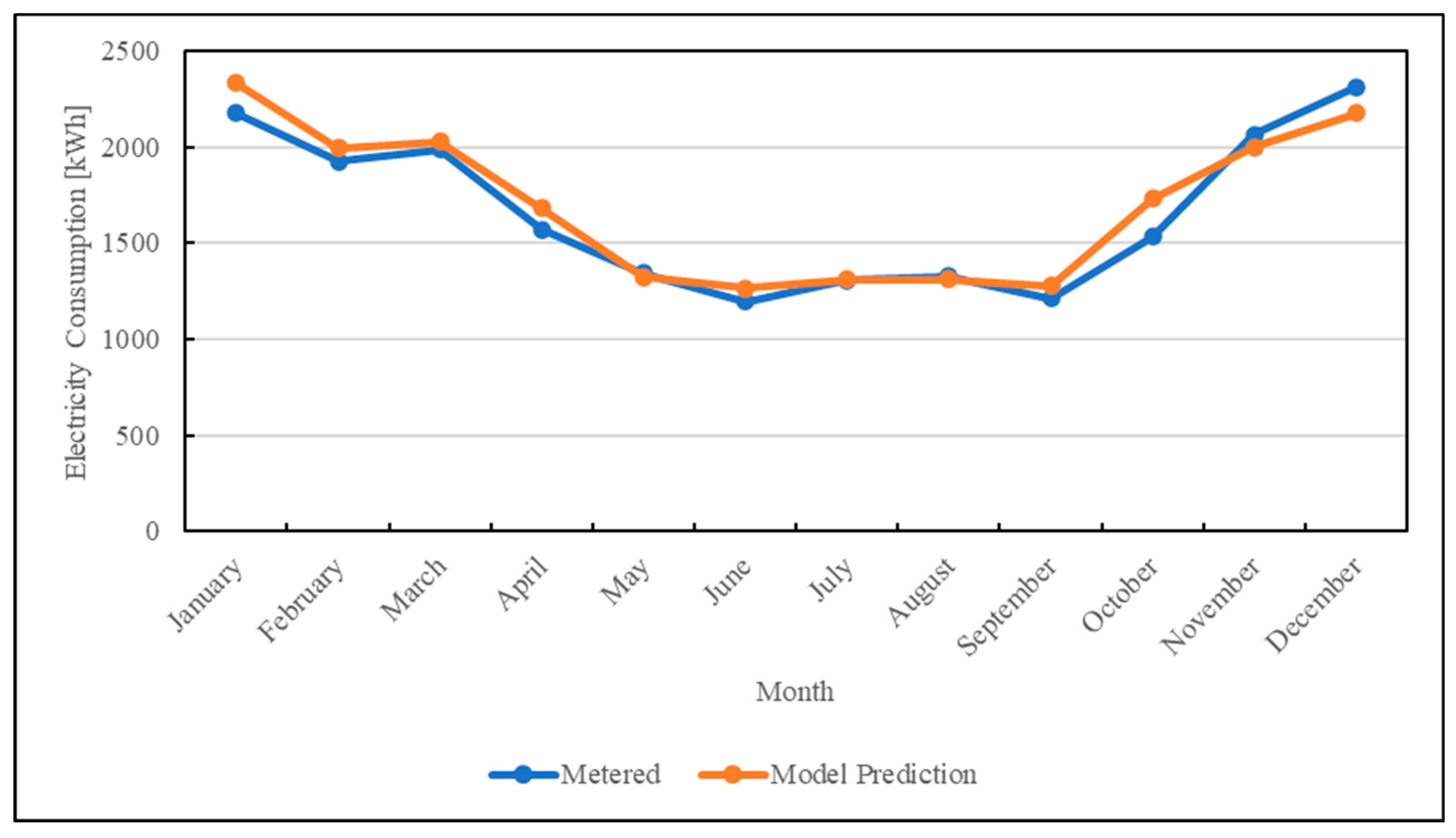
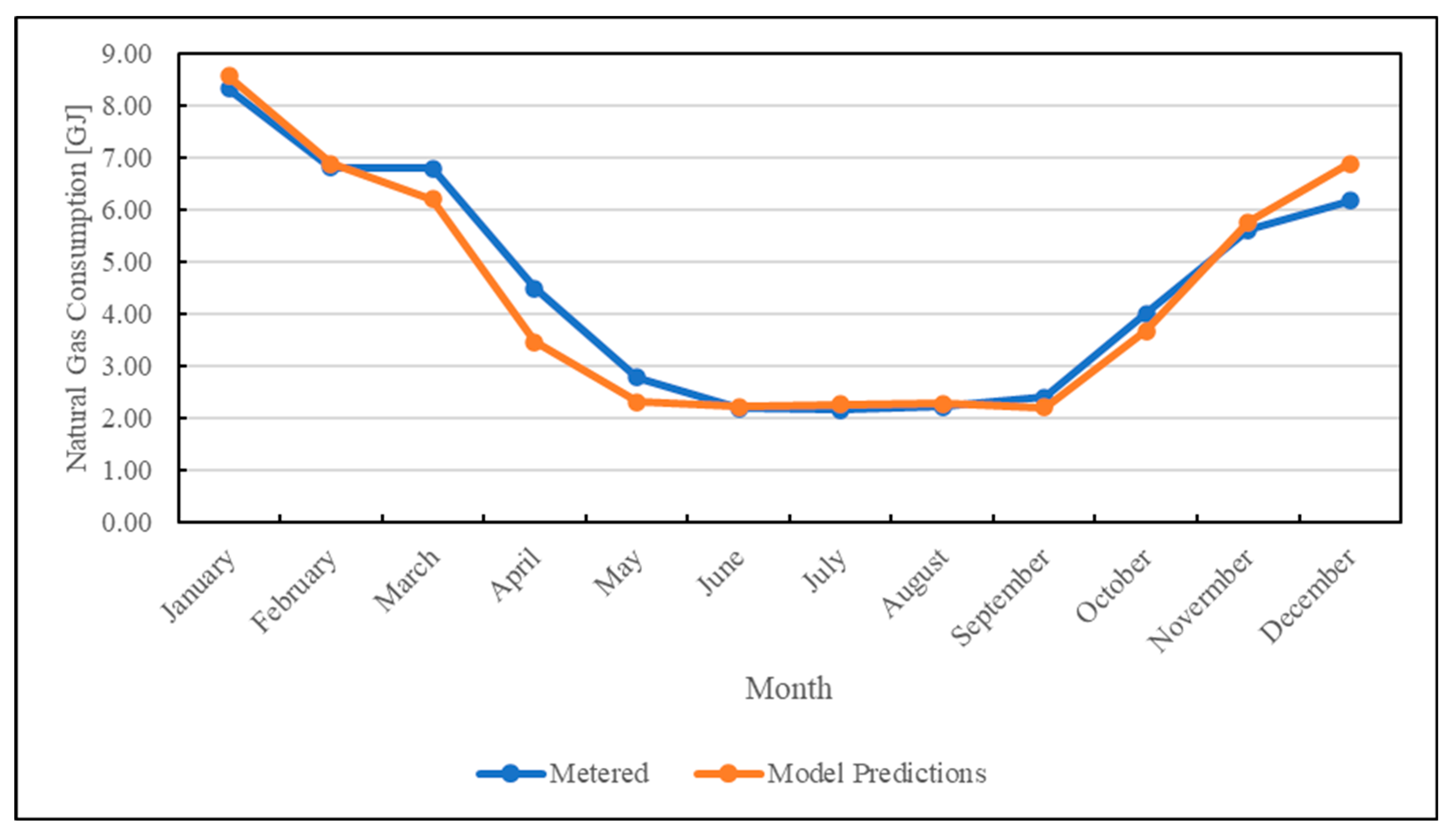
Total	75.49	56.70

present the simulated annual electricity and natural gas consumptions for the building’s main energy end-uses under both scenarios. The results indicate that the introduction of the HRV results in an annual electricity consumption of 75.49 GJ and natural gas consumption of 56.70 GJ. In contrast, without the HRV, the consumptions are 73.64 GJ for electricity and 52.70 GJ for natural gas. The increased electricity usage in the HRV scenario is primarily attributed to the operation of the HRV’s exhaust and supply air fans, which facilitates continuous ventilation by introducing fresh air into the space and exhausting indoor stale air outside the building. Figure 15 illustrates the comparison of natural gas consumption across main energy end-use between the two scenarios. As seen in the figure, the additional natural gas usage in the HRV scenario is predominantly attributed to the space heating end-use.

The increased natural gas consumption in the HRV scenario is primarily due to the additional heat loss associated with the mechanically ventilated air introduced by the HRV system. In the scenario without the HRV, the building is passively ventilated by intermittently running washroom exhaust fans, with windows assumed to remain closed during simulations. Consequently, infiltration is the sole source of outside air-induced heat loss of the building in this scenario. The infiltration-air-induced heat loss in the existing building, $Q_{inf.htg.ext}$, can be calculated using the following equation:

$$Q_{inf·htg}={\dot{m}}_{inf}\times C_p\times (T_{htg·sp}-T_o)$$

(4)

where

$Q_{inf·htg.ext}$ = infiltration-air-induced space heat loss in existing house, $\mathrm{k}\mathrm{W};$

${\dot{m}}_{inf}$ = mass flowrate of infiltrated air in existing building, $\mathrm{k}\mathrm{g}/\mathrm{s}$;

$C_p$ = specific heat capacity of air, $\mathrm{k}\mathrm{J}/\mathrm{k}\mathrm{g}·\mathrm{K}$;

$T_{htg·sp}$ = indoor heating setpoint temperature, $\mathrm{K};$

$T_o$ = outdoor dry bulb temperature, $\mathrm{K}$.

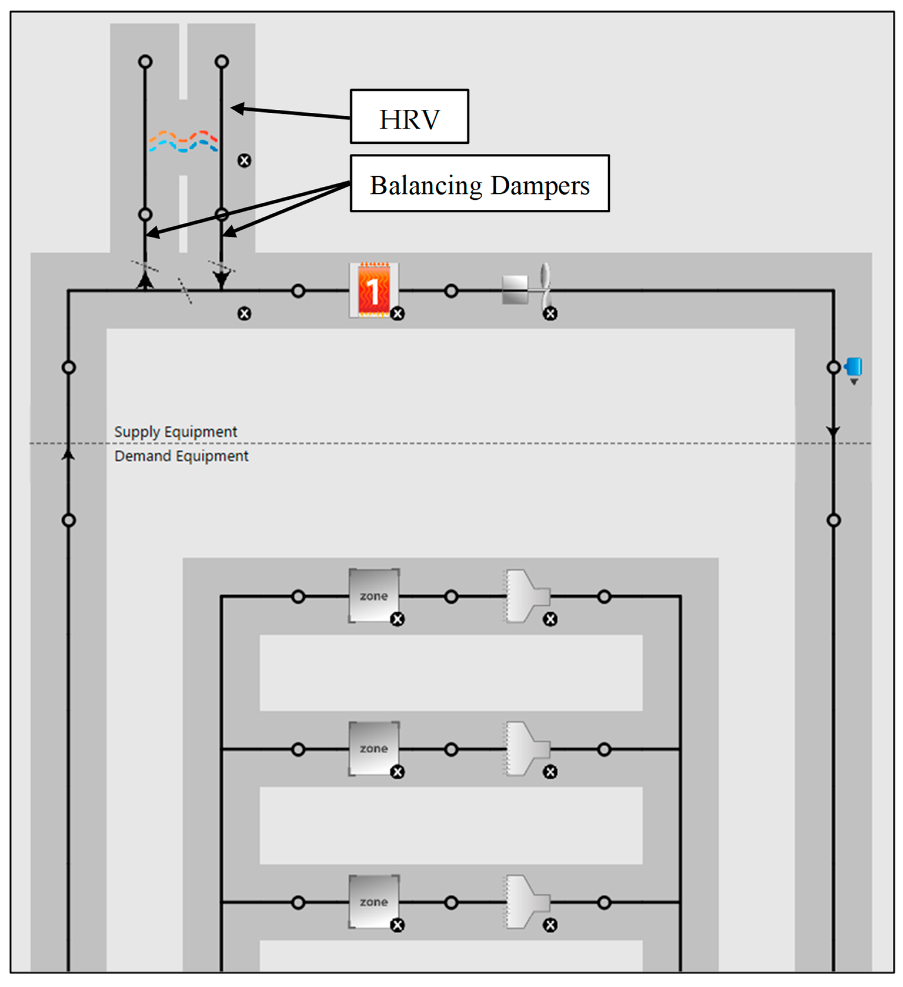
In contrast, the scenario with the HRV assumes a balanced ventilation system is added to the existing HVAC system to accommodate the deployment of the HRV. Thus, the HRV introduces outside air at a certain flowrate into the space, partially heating this air by harvesting waste the waste heat from the exhaust air stream passing through the HRV, depending on the HRV’s heat exchange effectiveness. Therefore, in the scenario with the HRV, both infiltration and mechanically ventilated air contribute the outside-air-induced building heat loss, $Q_{o.htg·hrv}$, which can be calculated as:

$$Q_{o.htg·hrv}=[{\dot{m}}_{ven·hrv}\times (1-\epsilon )+{\dot{m}}_{inf·hrv}]\times C_p\times (T_{htg·sp}-T_o)$$

(5)

where

$Q_{o.htg·hrv}$ = total outside-air-induced space heat loss after the HRV is applied, $\mathrm{k}\mathrm{W};$

${\dot{m}}_{ven·hrv}$ = rated mass flowrate of the HRV supply/exhaust fan, $\mathrm{k}\mathrm{g}/\mathrm{s}$;

$\epsilon$ = HRV heat exchange effectiveness, $fraction;$

${\dot{m}}_{inf·hrv}$ = mass flowrate of the infiltrated air in the with-HRV scenario, $\mathrm{k}\mathrm{g}/\mathrm{s}$;

$C_p$ = specific heat capacity of air, $\mathrm{k}\mathrm{J}/\mathrm{k}\mathrm{g}·\mathrm{K}$;

$T_{htg·sp}$ = indoor heating setpoint temperature, $\mathrm{K};$

$T_o$ = outdoor dry bulb temperature, $\mathrm{K}$.

In this study, the mass flowrate of infiltrated air remains the same (i.e., ${\dot{m}}_{inf}$ vs. ${\dot{m}}_{inf·hrv}$) in both scenarios. Equations (4) and (5) imply the outside air-induced heat loss in the with-HRV scenario must be greater than that in the without-HRV scenario since the heat exchange effectiveness of the HRV, $\epsilon$, is always less than unity (i.e., 100% efficiency). As a result, the space heating system in the with-HRV scenario consumes more natural gas than in the without-HRV scenario.

In order to balance the additional heat loss induced by the mechanically ventilated air passing through the HRV, the total outside air-induced space heat loss after HRV is applied, $Q_{o.htg·hrv}$, must be equal to or less than the infiltration air-induced space heat loss in the existing house, $Q_{inf·htg}$. Thus, by dividing the terms, $C_p\times (T_{htg·sp}-T_o)$ in both equations, we have:

$$\left[{\dot{m}}_{ven·hrv}\times \left(1-\epsilon \right)+{\dot{m}}_{inf·hrv}\right]={\dot{m}}_{inf}$$

(6)

Equation (6) implies that if the envelope air tightness after the deployment of the HRV can be improved to a level such that

$${\dot{m}}_{inf·hrv}<{\dot{m}}_{inf}-{\dot{m}}_{ven·hrv}\times \left(1-\epsilon \right)$$

(7)

then the total outside air-induced space heat loss in the with-HRV scenario will be smaller than that in the without-HRV scenario, resulting in reductions in building space heating energy consumption. This suggests that for an existing building without an active or balanced mechanical ventilation system in place, implementing an HRV should always be accompanied by the retrofit of building envelope systems to improve airtightness. In this study, the infiltration rate in the without-HRV scenario was modeled as 0.367 $ACH$ (i.e., ${\dot{m}}_{inf}$), while the ventilation air and the heat exchange effectiveness of the HRV in the with-HRV scenario were modeled as 0.367 $ACH$ (i.e., ${\dot{m}}_{ven·hrv}$) and 75.9% (i.e., $\epsilon )$, respectively. Thus, the infiltration rate of the building envelope after the HRV retrofit, ${\dot{m}}_{inf·hrv}$, needs to be equal to or less than 0.281 $ACH$, according to Equation (7), so that the implementation of the HRV will not lead to additional space heating energy use.

In the practice, if calculations indicate that achieving the required infiltration rate (i.e., ${\dot{m}}_{inf·hrv}$) after the HRV implementation is unrealistically low or non-existent (i.e., $\le 0$), that suggests that adding an HRV to the existing building heating system may result in increased space heating energy consumption. This scenario typically occurs in existing buildings with a relatively low infiltration rate; hence, it is essential to assess whether the building is under-ventilated by comparing the current infiltration airflow rate to the minimum ventilation airflow rate requirements specified by relevant codes and standards, such as AHRAE 62.2.

If the building does not meet these ventilation standards, the implementation of an HRV in existing HVAC system becomes essential to improve the indoor air quality. In such scenarios, when comparing space heating energy consumption between scenarios with and without an HRV, it is crucial to account for the improved indoor air quality conditions provided by the HRV. However, to avoid unnecessary over-ventilation, which can lead to increased space heating energy consumption, the HRV’s ventilation capacity should be carefully determined. Ideally, the HRV should only supply the additional outdoor airflow necessary to meet the minimum code required ventilation rate, compensating for any shortfall in the building’s natural infiltration. This approach ensures compliance with the ventilation standards while minimizing the outdoor air-induced energy usage.

If the building already meets the required ventilation standards through natural infiltration, the implementation of an HRV in existing building solely to improve the indoor air quality may not be necessary. In such cases, the building relies on passive ventilation, which is neither controllable nor preheated, potentially leading to increased space heating energy consumption. To address this, enhancing the building envelope airtightness is recommended before any retrofit with an HRV system. This approach minimizes the uncontrolled infiltration and allows the HRV to be sized appropriately to compensate for the reduced infiltration, while maintaining the desired indoor air quality levels.

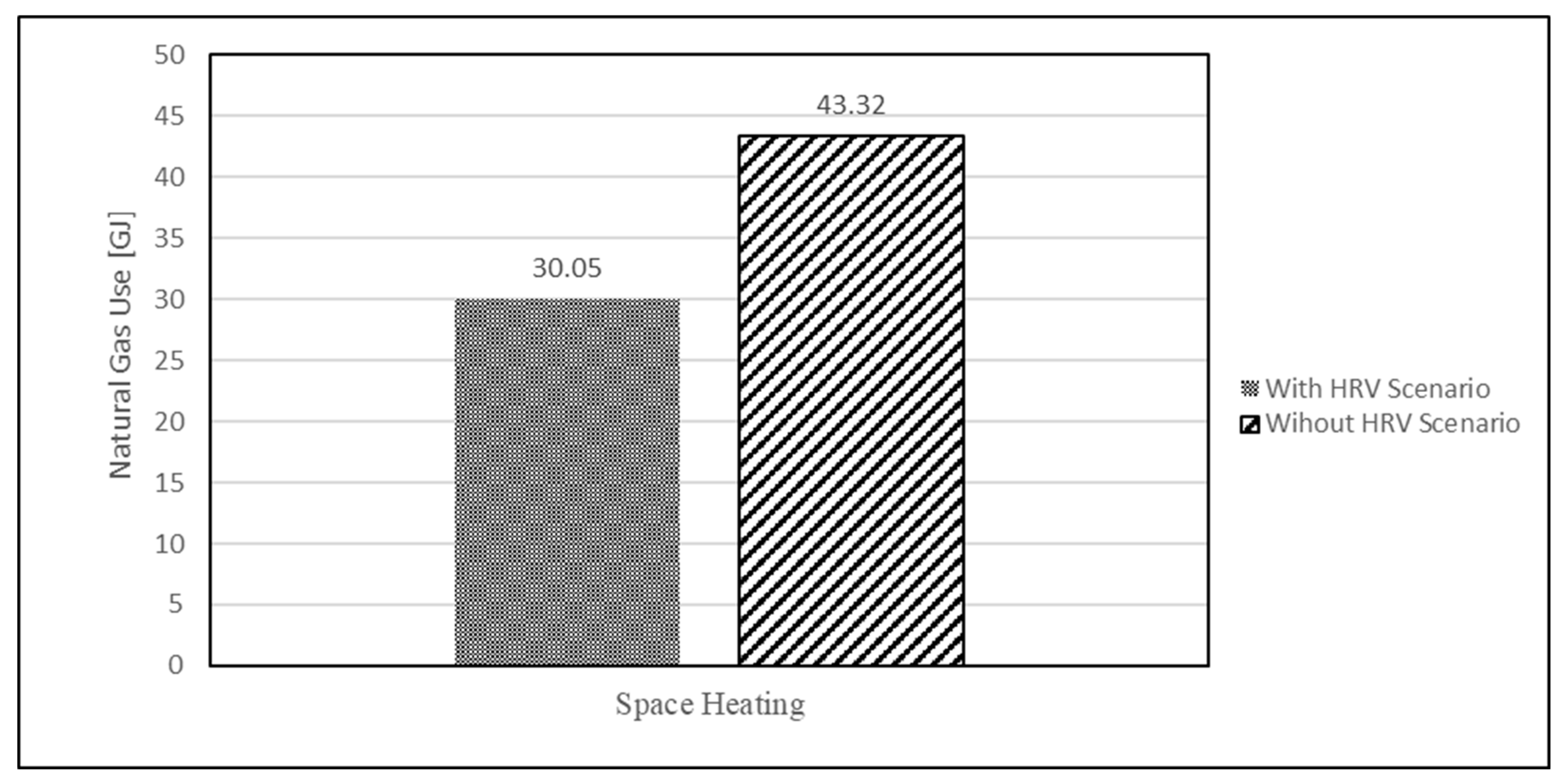
Figure 16 illustrates the comparison of the natural gas consumed by space heating systems coupled with and without the HRV under identical ventilation conditions. In this scenario, both the HRV’s ventilation air flow rate and infiltration air rate are set equally across both systems. As seen in the figure, the building space heating system equipped with an HRV consumes 30.05 GJ of natural gas, while the same system without implementing the HRV consumes 43.32 GJ. This suggests that for existing buildings with active or balanced mechanical ventilation systems in place, employing an HRV can significantly reduce space heating energy consumption.

5. Conclusions

The study investigates the feasibility of implementing an HRV in a single-family residence in Vancouver’s climate zone, utilizing a calibrated building energy model for the analysis. In this study, an OpenStudio^® model was developed and calibrated against actual monthly utility data, encompassing both electricity and natural gas consumption, to accurately represent the energy performance characteristics of the building’s existing MEP systems. A series of simulations was conducted to compare and analyze the energy consumption of space heating systems with and without the implementation of an HRV under various ventilation scenarios, specifically contrasting natural infiltration-driven passive ventilation with HRV-assisted mechanical ventilation. Key findings include:

• Impact of Implementing an HRV Without an Existing Balanced Mechanical Ventilation: Adding an HRV to an existing building without any active or balanced mechanical ventilation systems equipped may lead to an increased space heating energy consumption, compared with the existing heating system does.
• Recommendation for an Envelope Retrofit Prior to the HRV Retrofit: It is recommended to assess the building envelope’s airtightness using a blower door test before installing an HRV in buildings without active or balanced ventilation systems. Upgrading the envelope may be necessary to minimize uncontrolled infiltration and optimize the HRV sizing.
• Proper Sizing of the HRV: The HRV should be appropriately sized to compensate for any shortfall in the natural infiltration to ensure a sufficient indoor air quality while minimizing the outdoor-air-induced space heating energy usage.
• Break-even Infiltration Rate for HRV Retrofit for the Studied House: For the house in this study, achieving a break-even point of the infiltration rate of 0.281ACH is essential to ensure that implementing an HRV does not result in increased space heating energy consumption.
• Energy Savings with HRV Implementation Under Controlled Ventilation: When maintaining identical outdoor air flow rates, employing an HRV would always reduce space heating energy consumption.

6. Limitations and Future Work

In the study, the building energy model was calibrated by adjusting the values of certain input parameters. In addition to the space heating setpoint and the infiltration, values of the other parameters during the calibration were adjusted within a reasonable variation range due to the limited measurement data. Therefore, future studies could benefit from comprehensive field tests to gather more precise calibration data.

Additionally, in this work, the initial energy model of the building was calibrated against the building’s monthly aggregate electricity and natural gas consumption data; more granular calibration against the building’s main end-use energy measurements could enhance the model’s accuracy.

Lastly, the applicability of employing the HRV in the study was investigated by comparing the energy use of the space heating system with and without the HRV through the simulation. In other words, the HRV was not physically installed during the study and all the key energy performance characteristics of the HRV were input to the model based on the manufacturer provided specifications. This is because by the time of the study, the HRV has not been installed yet. In reality, the HRV’s run-time performance may be different from those published in the manual provided by the manufacturer. Therefore, in the future studies, it is necessary to conduct a field test to verify the real-world performance of the HRV.

References

1. United Nations Climate Change. The Paris Agreement. 2022. Available online: https://unfccc.int/process-and-meetings/the-paris-agreement/the-paris-agreement (accessed on 31 January 2022).
2. Government of Canada. Net-Zero Emissions by 2050. 22 January 2022. Available online: https://www.canada.ca/en/services/environment/weather/climatechange/climate-plan/net-zero-emissions-2050.html (accessed on 31 January 2022).
3. Government of Canada. Canada’s Actions to Reduce Emissions. 1 September 2020. Available online: https://www.canada.ca/en/services/environment/weather/climatechange/climate-plan/reduce-emissions.html (accessed on 21 January 2022).
4. Household Energy Consumption, by Type of Dwelling, Canada and Provinces. 1 April 2025. Available online: https://www150.statcan.gc.ca/t1/tbl1/en/tv.action?pid=2510006101 (accessed on 1 April 2025).
5. Government of Canada. Natural Resources Canada. 26 January 2022. Available online: https://oee.nrcan.gc.ca/corporate/statistics/neud/dpa/showTable.cfm?type=CP§or=res&juris=ca&rn=9&page=3 (accessed on 31 January 2022).
6. Wang, J.; Lonescu, D.; Hamer, G.; Bradley, D.; Hartman, M. Pathways to High-Performance Housing in British Columbia; Fpinnovations: Vancouver, BC, Canada, 2014. [Google Scholar]
7. Government of Canada. Energy Efficiency. 26 January 2022. Available online: https://www.nrcan.gc.ca/energy-efficiency/10832 (accessed on 31 January 2022).
8. Heat Pump Basics, 9 January 2025. Available online: https://natural-resources.canada.ca/energy-efficiency/electric-heat-pumps/heat-pump-basics#a2 (accessed on 1 April 2025).
9. Government of Canada. Variable Frequency Drives. 14 January 2025. Available online: https://natural-resources.canada.ca/energy-efficiency/energy-star/variable-frequency-drives (accessed on 1 April 2025).
10. U.S. Department of Energy. Chapter 5. In An Assessment of Energy Technologies and Research Opportunities; U.S. Department of Energy: Washington, DC, USA, 2015. [Google Scholar]
11. Burgess, J.; Bucket, N.; Camilleri, M.; Burrough, L.; Pollard, A. Papakowhai Retrofit Project—Improving the Thermal Envelope and Space Heating. In Proceedings of the SB10, Wellington, New Zealand, 26–28 May 2010. [Google Scholar]
12. FPInnovations. Guide for Designing Energy-Efficient Building Enclosuress for Wood-Frame Multi-Unit Residential Buildings in Marine to Cold Climate Zones in North America; FPInnovations: Vancouver, BC, Canada, 2013. [Google Scholar]
13. Omer, A.M. Renewable Building Energy Systems and Passive Human Comfort Solutions. Renew. Sustain. Rev. 2008, 12, 1562–1587. [Google Scholar] [CrossRef]
14. Liu, J.; Li, W.; Liu, J.; Wang, B. Efficiency of energy recovery ventilator with various weathers and its energy saving performance in a residential apartment. Energy Build. 2010, 42, 43–49. [Google Scholar] [CrossRef]
15. Zhong, K.; Chen, S.; Kang, Y.; Yuan, L. Analysis of outdoor temperature ranges for the operation of different ventilating modes in commercial buildings of China. Energy Build. 2012, 55, 174–182. [Google Scholar] [CrossRef]
16. El Fouih, Y.; Stabat, P.; Rivière, P.; Hoang, P.; Archambault, V. Adequacy of air-to-air heat recovery ventilation system applied in low energy buildings. Energy Build. 2012, 54, 29–39. [Google Scholar] [CrossRef]
17. Zhong, K.; Kang, Y. Applicability of air to air heat recovery in China. Appl. Therm. Eng. 2009, 29, 830–840. [Google Scholar] [CrossRef]
18. Li, B.; Wild, P.; Rowe, A. Performance of a heat recovery ventilator coupled with an air-to-air heat pump for residential suites in Canadian cities. J. Build. Eng. 2019, 21, 343–354. [Google Scholar] [CrossRef]
19. Lam, K.P.; Lee, S.R.; Dobbs, G.M.; Zhai, C. Simulation of the effect of an energy recovery ventilator on indoor thermal conditions and system performance. In Proceedings of the Ninth International IBPSA Conference, Montreal, QC, Canada, 15–18 August 2005. [Google Scholar]
20. Dodoo, A.; Gustavsson, L.; Sathre, R. Primary energy implications of ventilation heat recovery in residential buildings. Energy Build. 2011, 43, 1566–1572. [Google Scholar] [CrossRef]
21. Kang, Y.; Wang, Y.; Zhong, K.; Liu, J. Temperature ranges of the application of air-to-air heat recovery ventilator in supermarkets in winter, China. Energy Build. 2010, 42, 2289–2295. [Google Scholar] [CrossRef]
22. Zhou, Y.; Wu, J.; Wang, R. Performance of energy recovery ventilator with various weathers and temperature set-points. Energy Build. 2007, 39, 1202–1210. [Google Scholar] [CrossRef]
23. Barker, A.; Ramakrishnan, R. Parametric Analysis of Energy Recovery Ventilation Performance in the High-Rise Residential Sector: A Toronto Case Study; Toronto Metropolitan University: Toronto, ON, Canada, 2014. [Google Scholar]
24. Kim, S.-M.; Lee, J.-H.; Kim, S.; Moon, H.J.; Cho, J. Determining operation schedules of heat recovery ventilators for optimum energy savings in high-rise residential buildings. Energy Build. 2011, 46, 3–13. [Google Scholar] [CrossRef]
25. Roulet, C.-A.; Heidt, F.; Foradini, F.; Pibiri, M.-C. Real Heat Recovery with Air Handling Units. Energy Build. 2001, 33, 495–502. [Google Scholar] [CrossRef]
26. Homeowner Protection Office BC Housing. Heat Recovery Ventilation Guide for Houses; Homeowner Protection Office BC Housing: Vancouver, BC, Canada, 2015.
27. Zhou, Q.; Mukhopadhyaya, P. Design Versus Actual Energy Performance in Social Housing Buildings; BC Housing: Burnaby, BC, Canada, 2020. [Google Scholar]
28. Kneifel, J.; Payne, W.V.; Ullah, T.; Ng, L. Simulated Versus Measured Energy Performance of the NIST Net Zero Energy Residential Test Facility Design; National Institute of Standards and Technology: Gaithersburg, MD, USA, 2015. [Google Scholar]
29. Delfania, S.; Pasdarshahrib, H.; Karamic, M. Experimental investigation of heat recovery system for building air conditioning in hot and humid areas. Energy Build. 2012, 49, 62–68. [Google Scholar]
30. Mardiana-Idayu, A.; Riffat, S.B. An experimental study on the performance of enthalpy recovery system for building applications. Energy Build. 2011, 43, 2533–2538. [Google Scholar] [CrossRef]
31. Pekdogan, T.; Tokuç, A.; Ezan, M.A.; Başaran, T. Experimental investigation of a decentralized heat recovery ventilation system. J. Build. Eng. 2021, 35, 102009. [Google Scholar] [CrossRef]
32. Asdrubali, F.; Baldinelli, G.; Bianchi, F.; Cornicchia, M. Experimental performance analyses of a heat recovery system for mechanical ventilation in buildings. Energy Procedia 2015, 82, 465–471. [Google Scholar] [CrossRef]
33. Diao, Y.; Liang, L.; Kang, Y.; Zhao, Y.; Wang, Z.; Zhu, T. Experimental study on the heat recovery characteristic of a heat exchanger based on a flat micro-heat pipe array for the ventilation of residential buildings. Energy Build. 2017, 152, 448–457. [Google Scholar] [CrossRef]
34. Al-Zubaydi, A.Y.T.; Hong, G. Experimental investigation of counter flow heat exchangers for energy recovery ventilation in cooling mode. Int. J. Refrig. 2018, 93, 132–143. [Google Scholar] [CrossRef]
35. Jermyn, D.; Richman, R. A process for developing deep energy retrofit strategies for single-family housing typologies: Three Toronto case studies. Energy Build. 2016, 116, 522–534. [Google Scholar] [CrossRef]
36. Fleur, L.L.; Moshfegha, B.; Rohdin, P. Measured and predicted energy use and indoor climate before and after a major renovation of an apartment building in Sweden. Energy Build. 2017, 146, 98–110. [Google Scholar] [CrossRef]
37. Guglielmetti, R.; Macumber, D.; Long, N. OpenStudio: An Open Source Integrated Analysis Platform. In Proceedings of the Building Simulation 2011: 12th Conference of International Building Performance Simulation Association, Sydney, Australia, 14–16 November 2011. [Google Scholar]
38. Parker, A.; Macumber, D.; Benne, K. Building Energy Modeling with OpenStudio: A Practical Guide for Students and Professionals; Springer International Publishing: Gewerbestrasse, Switzerland, 2018.
39. ENERGY STAR Home Sealing Specification Version 1.0; ENERGY STAR: 2001. Available online: https://www.energystar.gov/ia/home_improvement/home_sealing/ES_HS_Spec_v1_0b.PDF?2075-0401#:~:text=Scope:,building%20envelope%20in%20existing%20homes (accessed on 1 April 2025).
40. U.S. Green Building Council. 13 November 2019. Available online: https://www.usgbc.org/resources/leed-v41-minimum-energy-performance-calculator (accessed on 19 April 2022).
41. Lawrence Berkeley National Laboratory Simulation Research Group. Building Energy Use and Cost Analysis Program; Lawrence Berkeley National Laboratory Simulation Research Group: Berkeley, CA, USA, 2018. [Google Scholar]
42. Canadian Commission on Building and Fire Codes National Research Council of Canada. National Energy Code of Canada for Buildings; Canadian Commission on Building and Fire Codes National Research Council of Canada: Ottawa, ON, Canada, 2017. [Google Scholar]
43. HVI Certified Products Directory. Home Ventilating Institute. 2022. Available online: https://www.hvi.org/hvi-certified-products-directory/section-iii-hrv-erv-directory-listing/ (accessed on 26 July 2022).
Figure 1. A 3D rendering of the studied house in SketchUp model. N is for the north direction.
Energies 18 01820 g001
Figure 2. Rooms on ground floor.
Energies 18 01820 g002
Figure 3. Rooms at second floor.
Energies 18 01820 g003
Figure 4. Schematic of supply air ductwork layout.
Energies 18 01820 g004
Figure 5. Heating system’s air loop logic network in OpenStudio.
Energies 18 01820 g005
Figure 6. Lighting schedule.
Energies 18 01820 g006
Figure 7. Miscellaneous load schedule.
Energies 18 01820 g007
Figure 8. Hot water usage schedule.
Energies 18 01820 g008
Figure 9. Space heating setpoint schedule.
Energies 18 01820 g009
Figure 10. Calendarized monthly electricity use of the house in 2020.
Energies 18 01820 g010
Figure 11. Calendarized monthly natural gas use of the house in 2020.
Energies 18 01820 g011
Figure 12. Air loop of the space heating system incorporating an HRV in the OpenStudio Model.
Energies 18 01820 g012
Figure 13. Comparison of monthly electricity consumption (kWh) between calendarized meter readings and model predictions following calibration.
Energies 18 01820 g013
Figure 14. Comparison of monthly natural gas consumption (GJ) between calendarized meter readings and model predictions following calibration.
Energies 18 01820 g014
Figure 15. Comparison of annual natural gas use by end-uses between with- and without-HRV scenarios.
Energies 18 01820 g015
Figure 16. Comparison of natural gas use between scenarios with and without HRV under identical ventilation conditions.
Energies 18 01820 g016