Article

A Bi-Level Capacity Optimization Method for Hybrid Energy Storage Systems Combining the IBWO and MVMD Algorithms

1
School of Intelligent Science and Engineering, Hubei Minzu University, Enshi 445000, China
2
Key Laboratory of Green Manufacturing of Super-Light Elastomer Materials of State Ethnic Affairs Commission, Hubei Minzu University, Enshi 445000, China
*
Author to whom correspondence should be addressed.
Energies 2025, 18(7), 1777; https://doi.org/10.3390/en18071777
Submission received: 25 February 2025 / Revised: 23 March 2025 / Accepted: 26 March 2025 / Published: 2 April 2025
(This article belongs to the Section A1: Smart Grids and Microgrids)

Abstract

:
With the swift evolution of renewable energy technologies, the design and optimization of microgrids have emerged as vital components for fostering energy transition and promoting sustainable development. This study presents a bi-level capacity optimization model for microgrids, integrating wind–solar generation with hybrid electric–hydrogen energy storage systems to simultaneously enhance economic efficiency and system stability. The outer layer minimizes the annual total cost through the application of an Improved Beluga Whale Optimization (IBWO) algorithm, which is enhanced by strategies including the reverse elitism strategy, horizontal and vertical crossover operations, and a whirlwind scavenging strategy to improve performance. The inner layer builds on the optimized results from the outer layer, employing a Multivariable Variational Mode Decomposition (MVMD) algorithm to regulate the power output of the energy storage system. By integrating electric–hydrogen hybrid storage technology, the inner layer effectively mitigates power fluctuations. Furthermore, this study designs a modal decomposition-based charging and discharging scheduling strategy to ensures the system’s continuous and stable operation. Simulations performed on MATLAB 2018b and CPLEX 12.8 platforms indicate that the proposed dual-layer model decreases annual total expenses by 27.5% compared to a single-layer model while keeping grid-connected power variations within 10% of the installed capacity. This research provides innovative perspectives on microgrid optimization design and offers substantial technical support for ensuring stability and economic efficiency in intricate operational settings.

1. Introduction

As global attention to sustainable development and the energy transition intensifies, microgrids are emerging as innovative solutions for energy management. By integrating renewable energy sources such as wind and solar power with energy storage systems, microgrids enable localized power generation and consumption, thereby enhancing energy efficiency while improving the reliability and flexibility of power systems [1,2]. In the operation of microgrids, capacity optimization plays a crucial role in influencing both the economic performance and the stability of the system. Consequently, the development of an effective capacity optimization model that addresses economic efficiency alongside system reliability remains a significant challenge in contemporary research.
Swarm intelligence optimization algorithms represent a class of heuristic methods inspired by the collective behaviors of animals in nature. These algorithms have been widely applied to address complex optimization problems [3,4]. Among them, Particle Swarm Optimization (PSO) has attracted considerable attention in recent years [5,6,7]. Additionally, other swarm intelligence algorithms have demonstrated outstanding capabilities in solving optimization challenges. For instance, Liu et al. introduced a multiobjective Ant Colony Optimization algorithm (ACO), which significantly improved both solution quality and computational efficiency [8]. Similarly, Fan et al. demonstrated the effectiveness of the Bat Algorithm (BA) in addressing complex optimization problems [9]. However, most existing studies primarily focus on economic efficiency as the sole objective, and the convergence accuracy still needs to be improved. They usually emphasize cost–benefit analysis while often neglecting the stability and sustainability of the system. This limitation may lead to system instability or even failure when faced with external fluctuations or unforeseen events. To address this issue, Huang et al. proposed a dual-objective optimization model that simultaneously considers economic and environmental benefits [10]. Wang et al. employed the Beluga Whale Optimization (BWO) algorithm, achieving significant reductions in system costs while enhancing stability [11]. Zhou et al. compared the BWO with other commonly used swarm intelligence optimization algorithms, such as PSO, ACO, and BA, in a microgrid system. The results demonstrated that BWO converges faster and achieves a lower optimal value, confirming its significant advantages in renewable energy system scheduling and cost reduction [12]. Although these approaches have successfully improved the economic performance and power supply reliability of microgrids [13,14], they often oversimplify the modeling of microgrids. In highly uncertain power system environments, algorithm stability and real-time scheduling capabilities require further refinement. In this context, the Improved Beluga Whale Optimization (IBWO) algorithm significantly enhances the adaptability and robustness of the optimization process. By establishing a bi-level optimization model aimed at economic efficiency and stability, the approach not only mitigates the risks associated with single-layer optimization models but also offers a practical solution for improving overall microgrid performance and addressing dynamic changes.
The intermittent nature of wind and solar energy often leads to significant power fluctuations within microgrids, resulting in degraded power quality, equipment damage, and system instability. Therefore, implementing effective measures to mitigate these fluctuations is critical for ensuring reliable microgrid operation. Modal decomposition techniques have gained substantial attention for their ability to decompose complex signals into simpler components, facilitating the identification and mitigation of key contributors to power fluctuations [15,16]. Common modal decomposition methods include Empirical Mode Decomposition (EMD), Variational Mode Decomposition (VMD), and Multivariate Variational Mode Decomposition (MVMD) [17]. While both VMD and EMD exhibit strong performance in power smoothing, their performance is highly sensitive to parameter settings, particularly the number of decomposition modes and frequency boundaries. This reliance on empirical parameter selection can lead to suboptimal optimization outcomes [18,19]. To address these limitations, Feng et al. proposed a Multiscale Variational Mode Decomposition (MVMD) method, which has demonstrated effectiveness in real-time fault detection [20]. Zhang et al. and Li et al. independently validated the advantages of MVMD in microgrid stability analysis, demonstrating its effectiveness in frequency band separation, noise reduction, and maintaining stable system power in large-scale microgrids. Compared with traditional VMD and EMD methods, MVMD exhibits superior adaptability by dynamically adjusting the number of modes to accommodate varying power fluctuation characteristics. This capability enables MVMD to provide stable power smoothing in response to changes in wind speed and solar radiation, ensuring an optimal balance between efficiency and stability. Consequently, MVMD serves as a crucial tool for enhancing microgrid stability analysis and optimizing power quality [21,22,23,24].
Furthermore, optimizing energy storage scheduling further enhances the power quality of microgrids [25]. Hybrid energy storage technology has emerged as an effective solution to address the volatility and load imbalance inherent in microgrids [26]. While individual energy storage systems, such as flywheel energy storage [27], lithium batteries [28], and supercapacitors [29], each offer distinct advantages in load response and power quality improvement, they are limited in their ability to meet rapidly fluctuating load demands. By integrating high energy density with high power responsiveness, hybrid energy storage technology significantly improves the efficiency of energy storage and release, ensuring stable frequency and voltage regulation within microgrids [30,31]. Krishnan et al. demonstrated the use of supercapacitors to compensate for the power discrepancies that traditional low-pass filters fail to address [32]. Liang et al. proposed a collaborative control method combining lithium-ion batteries and supercapacitors, which enhanced the dynamic response capabilities of microgrids [33]. However, supercapacitors, due to their relatively low energy density, are inadequate for large-scale, long-term energy storage needs. To address these limitations, Tang et al. proposed an energy management framework for photovoltaic grids based on electro-hydrogen hybrid energy storage [34]. Similarly, Liao et al. emphasized the critical role of hydrogen energy storage in capacity optimization and sensitivity analysis [35]. Studies indicate that hybrid energy storage systems, when integrated with hydrogen storage technology, are particularly effective in providing high-power support. This integration makes them well suited for large-scale, long-duration energy storage applications, especially in scenarios involving renewable energy sources with high volatility, such as wind and solar power [36,37]. In summary, in order to better highlight the advantages and limitations of different existing research methods, a brief comparative analysis is conducted in Table 1.
To balance economic efficiency and stability in microgrids, this paper proposes a bi-level capacity optimization model for a solar-wind-based electric–hydrogen hybrid energy storage system. The outer layer employs the IBWO algorithm for capacity planning, while the inner layer utilizes the MVMD algorithm to achieve power smoothing. The system is evaluated based on the curtailment rate, integrating hybrid energy storage technologies with modal decomposition-based charging and discharging strategies to ensure reliable and stable operation. Experimental results demonstrate the model’s significant advantages in optimizing the utilization of wind and solar energy resources, thereby enhancing the efficiency and stability of microgrid performance. The main contributions of this study are as follows:
(1)
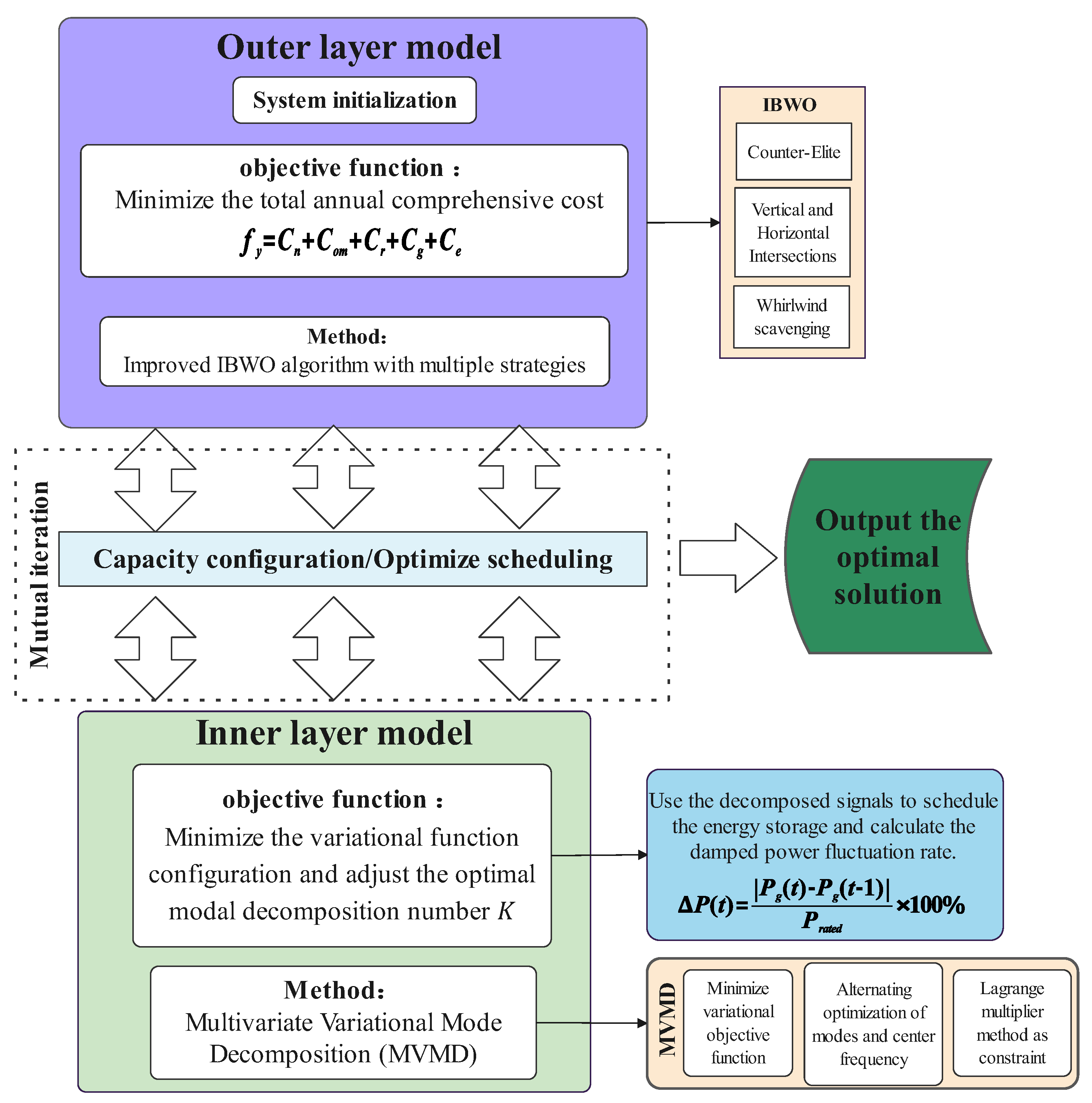
The bi-level optimization model achieves an optimal balance between the configuration of the energy storage system and the scheduling strategy through the coordinated optimization of both the inner and outer layers. This results in an operational solution that effectively balances economic considerations with stability.
(2)
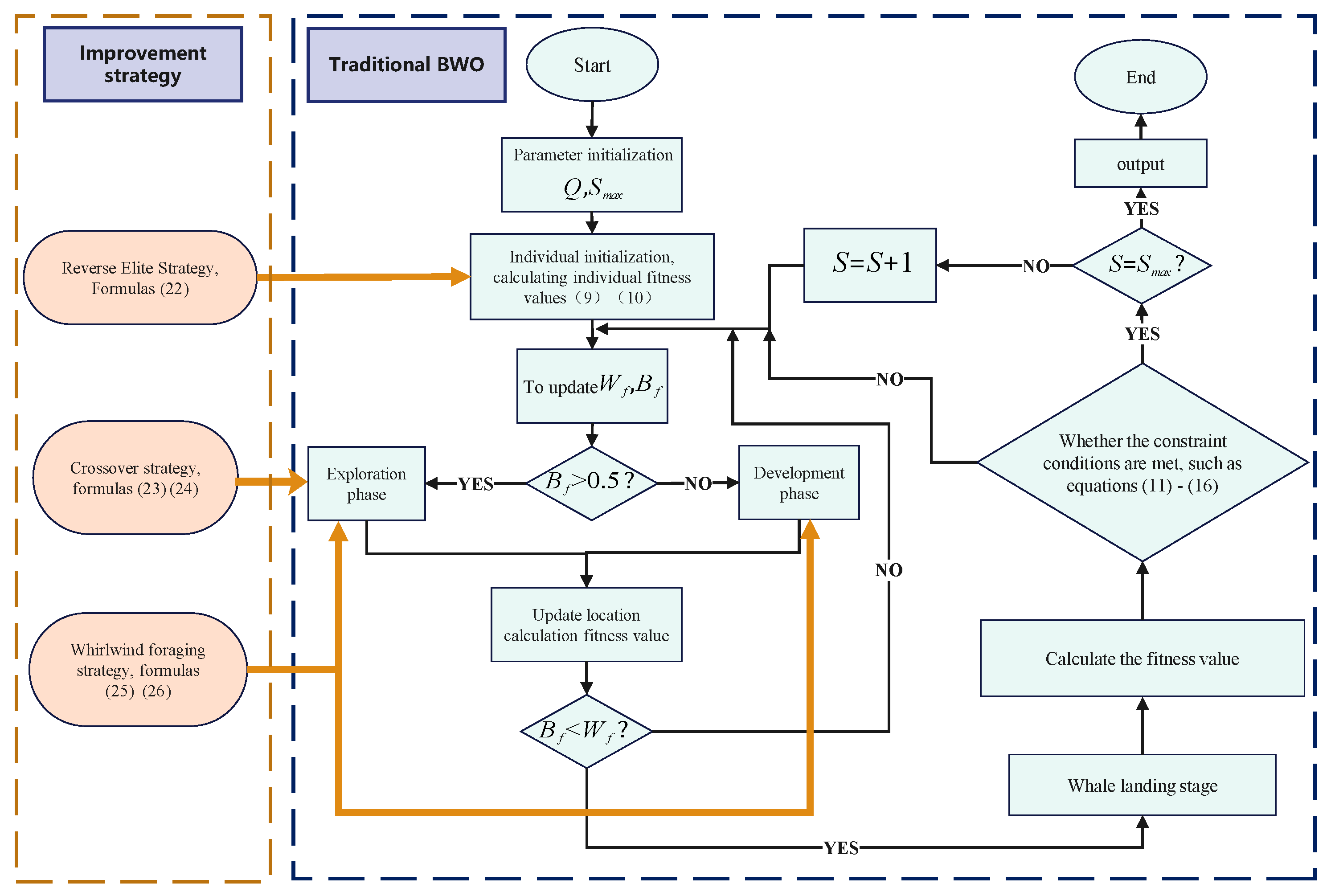
The IBWO incorporates the reverse elite strategy, vertical and horizontal crossover, and whirlwind scavenging strategy. These enhancements increase population diversity, facilitate global exploration, and mitigate the risk of local optima. Consequently, this method demonstrates improved speed and accuracy compared to three other widely used algorithms.
(3)
The electric–hydrogen hybrid storage technology is integrated with modal decomposition-based scheduling. By employing the MVMD algorithm to decompose power signals, batteries can swiftly respond to short-term load fluctuations, while the hydrogen storage offers substantial power support for large-scale, long-duration storage. This combination significantly enhances both the efficiency and the reliability of the microgrid.

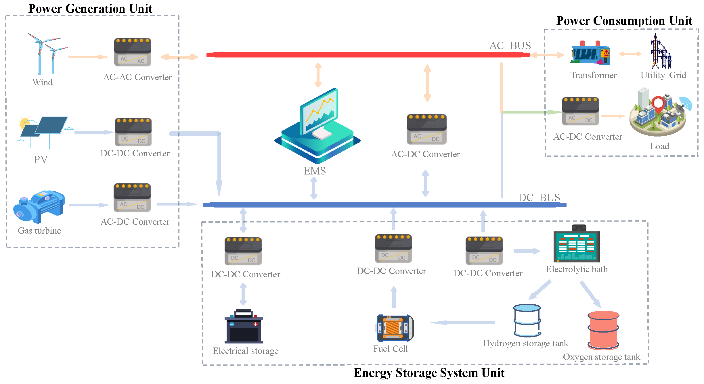
2. Wind–Solar–Hybrid Energy Storage of Microgrid Model

This paper presents a bi-level optimization model for grid-connected microgrids that incorporates electro-hydrogen hybrid energy storage technology to enhance power generation and storage efficiency. The model not only meets internal load demands and promotes energy self-circulation but also channels surplus power back into the grid, establishing an external loop that significantly enhances the overall energy efficiency of the system. The microgrid consists of a generation system, an energy storage system, loads, and an Energy Management System (EMS). The generation system incorporates photovoltaic panels, wind turbines, and gas turbines as backup power units. The energy storage system comprises batteries, hydrogen tanks, oxygen tanks, fuel cells, and an electrolytic cell. The detailed structure of the microgrid is depicted in Figure 1, with relevant parameters and their definitions provided in Table 2.

2.1. Wind Power Generation Model

The operation of a wind turbine is based on the principle of converting mechanical energy into electrical energy. The output power of a wind turbine is shown in Formula (1).
P w t ( v ) = 0 , 0 v < v c i Pr v 2 v c i 2 v r 2 v c i 2 , v c i v v r P r , v r < v v c o 0 , v c o < v

2.2. Photovoltaic System Model

The output power of a photovoltaic (PV) panel is affected by both the intensity of solar irradiance and the operating temperature of the panel, as shown in Formula (2).
P p v = f p v P S T C G G S T C 1 + P T T S T C T = T a + 30 × G 1000
In Equation (2), f p v is typically taken as 0.9; P is typically taken as −0.47%/°C.

2.3. Battery Model

The battery, which functions as a crucial energy storage and compensation module within microgrids, experiences a significant impact on its lifespan due to the depth of discharge. To promote the longevity of the battery, it is vital to avoid both overcharging and deep-discharging. The processes of charging and discharging the battery are described by Formula (3).
S O C t = 1 δ S O C t 1 + P c Δ t η c E c S O C t = 1 δ S O C t 1 P c Δ t η d E c
The battery capacity at time t is determined by the capacity at the previous time step and the charging and discharging power, as shown in Formula (4).
E b a t t = 1 δ E b a t t 1 + P c t η c P d t η d

2.4. Hydrogen Energy Storage Model

When surplus electricity is available, an electrolytic cell is employed to split water into hydrogen and oxygen for storage. The oxygen produced can potentially be sold to generate additional revenue. During periods of electricity shortages, the stored hydrogen is converted back into electricity using a fuel cell to meet the load demand. The output power of the electrolytic cell and fuel cell are shown in Formula (5).
P e l e tan k = P e l e · η e l e P F C D C = P tan k F C · η F C
The energy stored in the hydrogen storage tank at time t depends on the energy at the previous time step and the charging or discharging power, as shown in Formula (6).
E tan k t = E tan k t 1 + P e l e tan k t · Δ t P tan k F C · Δ t · η s t o r

2.5. The Model of the Microgas Turbine

The gas turbine generates electricity by consuming fuel, and its output is shown in Formula (7).
η M T t = 0.0753 P M T t 65 3 0.3095 P M T t 65 2 + 0.4174 P M T ( t ) 65 + 0.1068
During operation, the gas turbine incurs fuel costs, operation and maintenance costs, as well as pollutant treatment costs. The calculation formulas for these costs are provided in Formula (8).
C M T . O M t = K O M P M T t C M T . F t = C L H V P M T t η M T t C M T . E N t = k = 1 n C k γ m t , k P M T t

3. The Bi-Level Optimization Model for Microgrids

The bi-level model, integrated with a predictive control algorithm, effectively coordinates internal resources and external power scheduling. In the outer layer, an Improved Beluga Whale Optimization (IBWO) algorithm, which incorporates multiple strategies, is employed to optimize energy storage capacity. The inner layer, guided by the optimization results from the outer layer, utilizes the Multivariable Variational Mode Decomposition (MVMD) algorithm to regulate the power output of the storage system. Through iterative optimization across both layers, the model achieves an optimal operational solution that balances economic efficiency with system stability. The two-layer optimization model is illustrated in Figure 2, with relevant parameters and their definitions detailed in Table 3.

3.1. Outer Layer Optimization Model

3.1.1. Outer Objective Function

The outer objective function aims to minimizes the annual comprehensive cost, which encompasses the initial construction costs, operation and maintenance costs, replacement costs, power grid transaction costs, and environmental protection costs. The function is shown in Formulas (9) and (10).
f y = C n + C o m + C r + C g + C e
C n = i = 1 n N i c i n S i n a 1 + a Y i 1 + a Y i 1 C o m = i = 1 n N i c i o m S i n C r = i m N i c i r S i n r 1 + r Y i 1 C g = 0 T k b u y P b u y t d t 0 T k s e l l P s e l l t d t C e = t = 1 T k = 1 n ( C r β g r i d , r ) P b u y t + C M T . E t + C D E . E N t
In Formula (10), a is the discount rate, taken as 0.05.

3.1.2. Outer Constraints

(1) The power balance constraint.
During the operation of the system, it is necessary to always meet the power balance constraint, that is, to balance the generated power with the consumed power. The power generated by the system includes the power generated by photovoltaic, wind and gas turbines, the discharge power of batteries and fuel cells, and the power purchased and sold by the power grid. The main power consumption of the system is the load and energy storage charging power.
P w t + P P V + P B A T + P F C + P g r i d + P M T = P e l + P l o a d
(2) Power constraints on wind turbines and photovoltaic output.
0 P w t t P w t max 0 P P V t P P V max
(3) Battery charging and discharging constraints.
S O C min S O C t S O C max 0 P c t P c max 0 P d t P d max
(4) Hydrogen energy storage system constraints.
0 P e l t P e l max 0 P F C t P F C max E tan k min t E tan k t E tan k max t
(5) Output constraints of microgas turbines.
P M T min t P M T t P M T max t P M T t P M T t 1 β M T
(6) Power constraints for purchasing and selling electricity.
P b u y P g r i d max P s e l l P g r i d max

3.2. Inner Layer Optimization Model

3.2.1. Inner Objective Function

The inner objective function is the power fluctuation rate after mixed energy storage stabilization. First, calculate the power before stabilization minus the power after stabilization, and then characterize it by the ratio of its rated power. The function is expressed by Formula (17).
Δ P t = P g t P g t 1 P r a t e d × 100 %

3.2.2. Inner Constraint

(1) The power fluctuation rate constraint.
The power fluctuation constraint is that the active power fluctuation interval within one minute shall not exceed 10% of the installed capacity.
Δ P Δ P max
(2) Hydrogen energy storage and battery charging and discharging constraints.
To avoid overcharging or over-discharging energy storage systems, which could impact their lifespan, charging and discharging constraints are specified in Formulas (13) and (14) under the outer constraints.

3.3. Evaluating Indicator

The renewable energy waste rate is a critical metric for evaluating the power generation capacity and self-balancing ability of microgrids. It reflects the proportion of renewable energy that is not utilized effectively due to scheduling challenges, insufficient load, or grid access restrictions. Regular monitoring and analysis of waste rates can optimize system strategies, enhance energy storage configurations, and develop flexible grid connection policies, thereby improving economic efficiency and promoting environmental sustainability. The waste rate is calculated by Formulas (19) and (20).
σ = P a b P t o × 100 %
P t o = i = 1 n P max , i × t P a b = P t o P a c

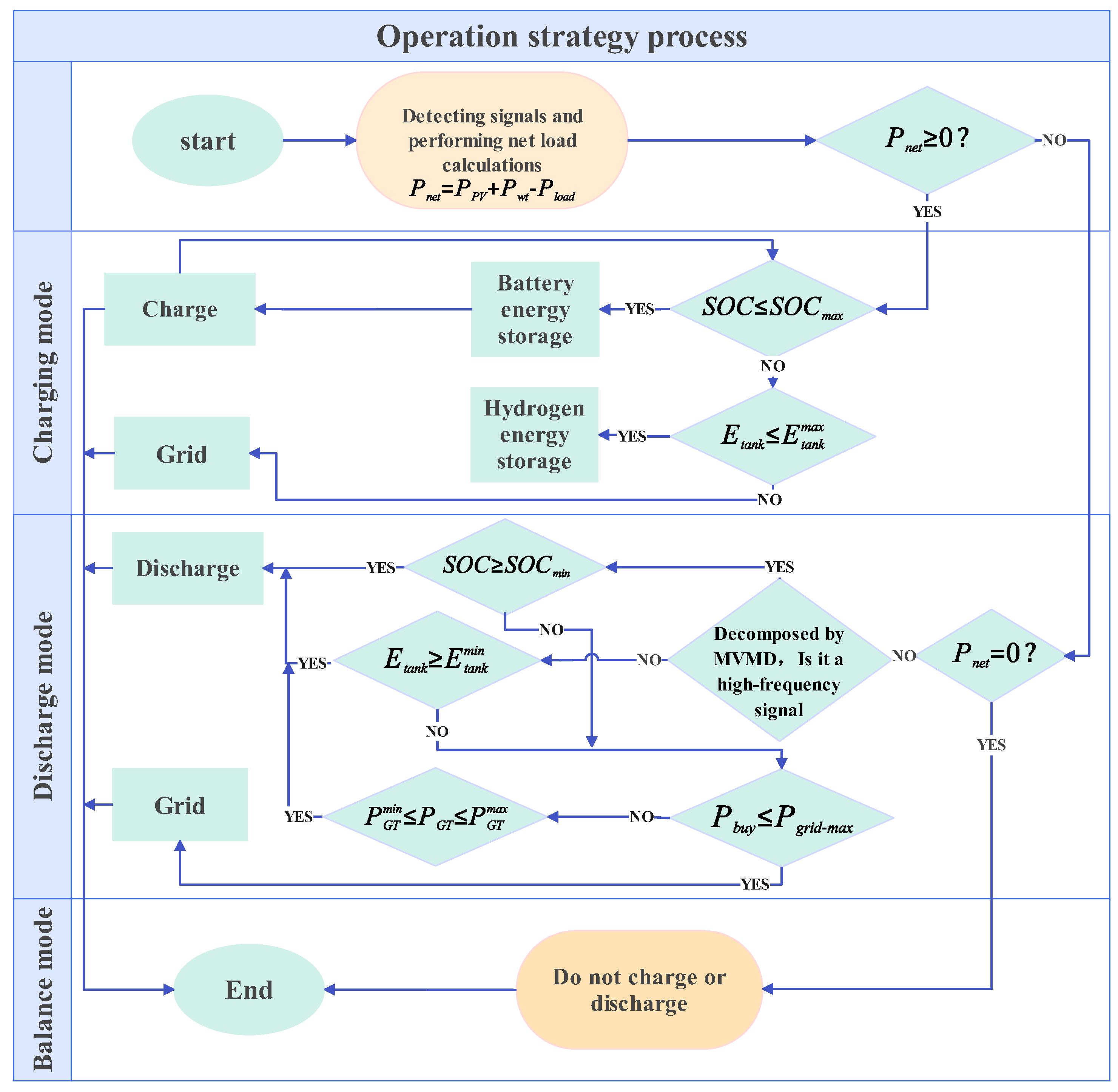
3.4. Operation Strategy

This study presents a hybrid energy storage operation strategy utilizing the Multivariable Variational Mode Decomposition (MVMD) algorithm. The MVMD algorithm effectively decomposes load demand and fluctuations in renewable energy generation, such as photovoltaic and wind power, into components of varying frequencies. During the operation of the microgrid in conjunction with the main grid, batteries are employed to mitigate high-frequency fluctuations, while hydrogen storage addresses mid- to low-frequency fluctuations. By incorporating predictive control algorithms, the charging and discharging strategies are optimized, facilitating advanced scheduling of batteries, hydrogen storage, and gas turbines to ensure optimal system performance. Net load is the difference between the power generated by photovoltaic and wind power and the power consumed by the load. The specific operational strategy is depicted in Figure 3, with the corresponding net load calculation formula provided by Formula (21).
P n e t = P P V + P w t P l o a d

4. IBWO

BWO is a heuristic algorithm inspired by the hunting behavior of beluga whales [38], which has demonstrated good performance in optimization problems. However, this algorithm is limited by premature convergence, which prevents it from fully exploring the solution space and missing potentially better solutions. To address this issue, this paper proposes a multistrategy improved BWO algorithm that integrates a reverse elitist strategy, a vertical and horizontal crossover operation, and whirlwind scavenging strategy to enhance its application effectiveness in multiobjective optimization problems.

4.1. Reverse Elite Strategy

The traditional BWO algorithm initializes the population randomly, which can lead to an uneven distribution across the solution space and negatively affect the algorithm’s performance. To mitigate this limitation, this paper introduces a reverse elitism strategy. During the initialization phase, information from elite individuals is utilized to construct the population in reverse, thereby enhancing the diversity and breadth of the search space, as in Formula (22).
X ˜ = u b + l b X X = x 1 , x 2 , , x n X ˜ = x ˜ 1 , x ˜ 2 , , x ˜ n
In Formula (22), u b is the upper limit of the interval, and l b is the lower limit of the interval.

4.2. Vertical and Horizontal Crossover Operation

To prevent the BWO algorithm from gradually converging to a local optimum during the iterative process, leading to premature convergence, a vertical and horizontal crossover strategy is introduced. This strategy enhances the global exploration capability, thereby preventing the occurrence of the “prematurity” phenomenon.

4.2.1. Horizontal Crossover Operation

The essence of horizontal crossover is that individuals learn from one another within the same dimension. Specifically, two distinct whale individuals are randomly selected to ensure that the crossover operation is not repeated. A crossover probability P h is then set to execute the crossover operation. After the crossover, the population is updated, and the best individuals are preserved through competitive evaluation between the parent and offspring generations, as shown in Formula (23).
M i , d o f s = φ 1 · F i , d + 1 φ 1 · F j , d + σ 1 · ( F i , d F j , d ) M j , d o f s = φ 2 · F j , d + 1 φ 2 · F i , d + σ 2 · ( F j , d F i , d )
In Formula (23), φ 1 and φ 2 are random numbers in the interval [0, 1], σ 1 and σ 2 are random numbers in the interval [−1, 1], F i , d and F j , d are the parent individuals in the d-th dimension, and M i , d o f s and M j , d o f s are the offspring produced by crossover in the d-th dimension.

4.2.2. Vertical Crossover Operation

The essence of vertical crossover lies in individuals learning from one another across various dimensions. By setting a crossover probability P v , the algorithm can escape local optima in dimensions where it may be stuck, thereby enhancing global search ability. After the crossover operation, both the parent and offspring engage in competition to preserve the most advantageous individuals, as shown in Formula (24).
M b e s t , d o f s = λ · F b e s t , d 1 + 1 λ · F b e s t , d 2
In Formula (24), M b e s t , d o f s is the offspring individual generated from the vertical crossover of parent individual F b e s t in dimensions d 1 and d 2 , and λ is a random number in the interval [0, 1].

4.3. Whirlwind Scavenging Strategy

The whirlwind scavenging strategy is introduced to guide individuals along a spiral trajectory toward the target, thereby accelerating the convergence process. This strategy effectively enhances the convergence rate of both local exploitation and global exploration. The corresponding calculations are shown in Formulas (25) and (26).
X i d t + 1 = x b e s t d t + r · ( x b e s t d t x i d t ) + δ · ( x b e s t d t x i d t ) , i = 1 x b e s t d t + r · x i 1 d t x i d t + δ · x b e s t d t x i d t , i = 2 , , N
δ = 2 e r 1 S max S + 1 S max · sin 2 π r 1
In Formulas (25) and (26), X i d t + 1 is the new position of the i-th beluga whale at time (t + 1), S is the number of iterations, S max is the maximum number of iterations, δ is the weighting coefficient, and r 1 is a random number in the interval [0, 1].

4.4. The Optimization Process of IBWO

The detailed optimization process of IBWO is illustrated in Figure 4. Q represents the population size, B f is the balance factor, B f = B 0 · ( 1 0.05 S / S max ) , B 0 is a random number in the interval [0, 1], and W f is the probability of whale fall, W f = 0.1 0.05 S / S max .

5. MVMD

The primary issue with the traditional VMD algorithm is the necessity to artificially specify the number of modes, represented by K. Setting k too small can lead to frequency aliasing, while setting it too large may result in spurious modes, affecting both analysis and control. Therefore, selecting the appropriate k is crucial. In this paper, an adaptive Multivariable Variational Mode Decomposition (MVMD) algorithm is proposed, which automatically adjusts the number of modes based on the characteristics of power fluctuations. This approach decomposes complex signals into multiple intrinsic mode functions, each representing a specific frequency component, ensuring optimal decomposition and meeting load demands.

5.1. Formulation of the Variational Problem

The core objective of the MVMD algorithm is to minimize the variational objective function, which contains multiple input signals and their corresponding modes.
min u k , ω k k t δ t + j π t · u k t e j ω k t 2 2 s . t . k u k t = f t u k t = A k t cos ϕ k t ω k t = ϕ k t = d ϕ k t d t
In Formula (27), u k = u 1 , u 2 , u k is the set of all modal components, ω k = ω 1 , ω 2 , , ω k is the set of all center frequencies, A k t is the amplitude of IMF, ϕ k t is the phase, and ω k t is the instantaneous frequency.

5.2. Solution of Variational Problem

In order to ensure the accuracy and stability of signal reconstruction, the Lagrange multiplier is introduced into the MVMD algorithm, and constraint conditions are introduced through the following Lagrange functions, as shown in Formula (28).
L u k , ω k , λ = α k t δ t + j π t · u k t e j ω k t 2 2 + f t k u k t 2 2 + λ t , f t k u k t
The updated modal formula of the frequency domain and center frequency are shown in Formulas (29) and (30).
u ^ k n + 1 ω = f ^ ω i k u ^ i n + 1 ω + λ ^ ω 2 1 + 2 α ω ω k 2
ω k n + 1 = 0 ω u ^ k ω 2 d ω 0 u ^ k ω 2 d ω

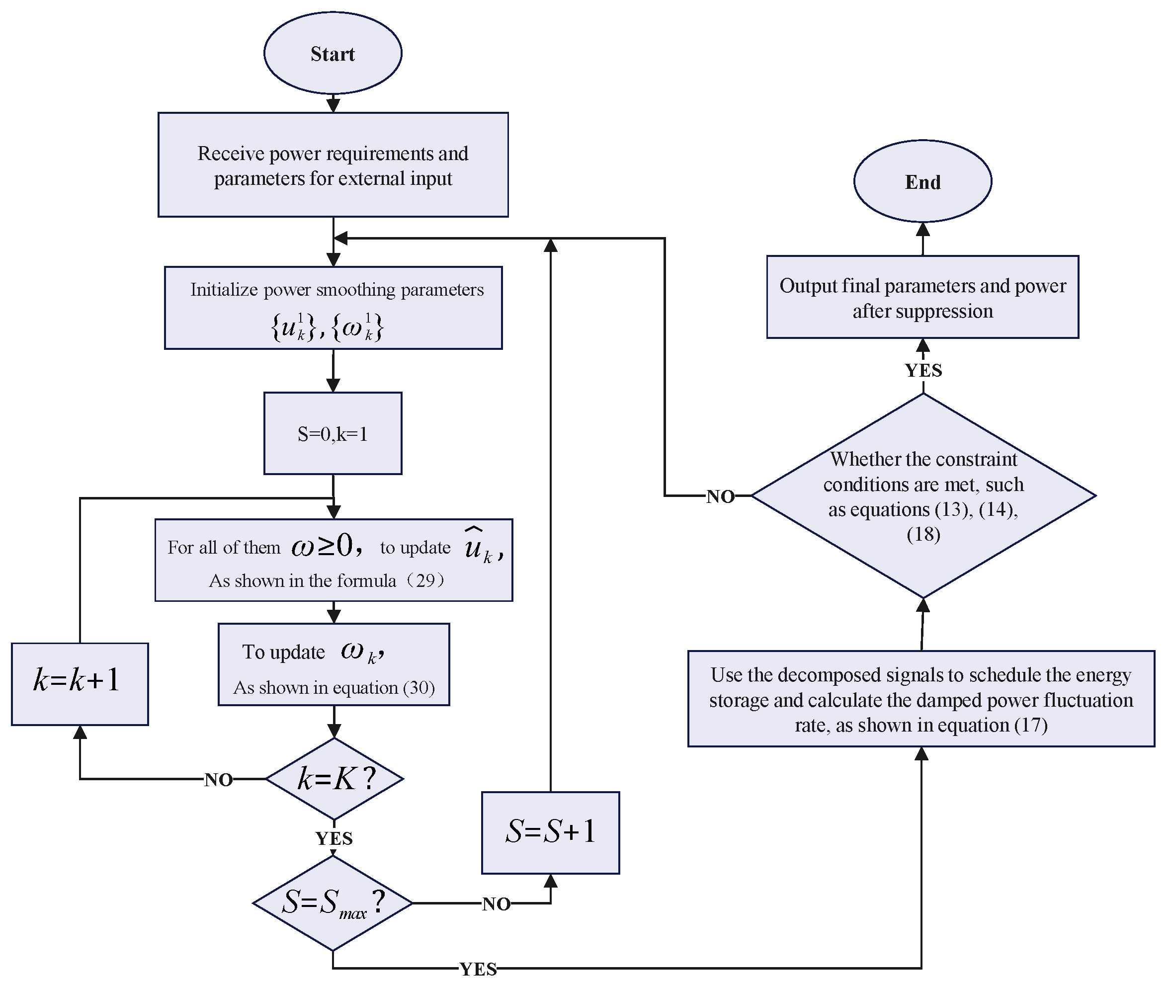
5.3. Optimization Process of MVMD

The detailed optimization process of MVMD is shown in Figure 5.

6. Example Analysis

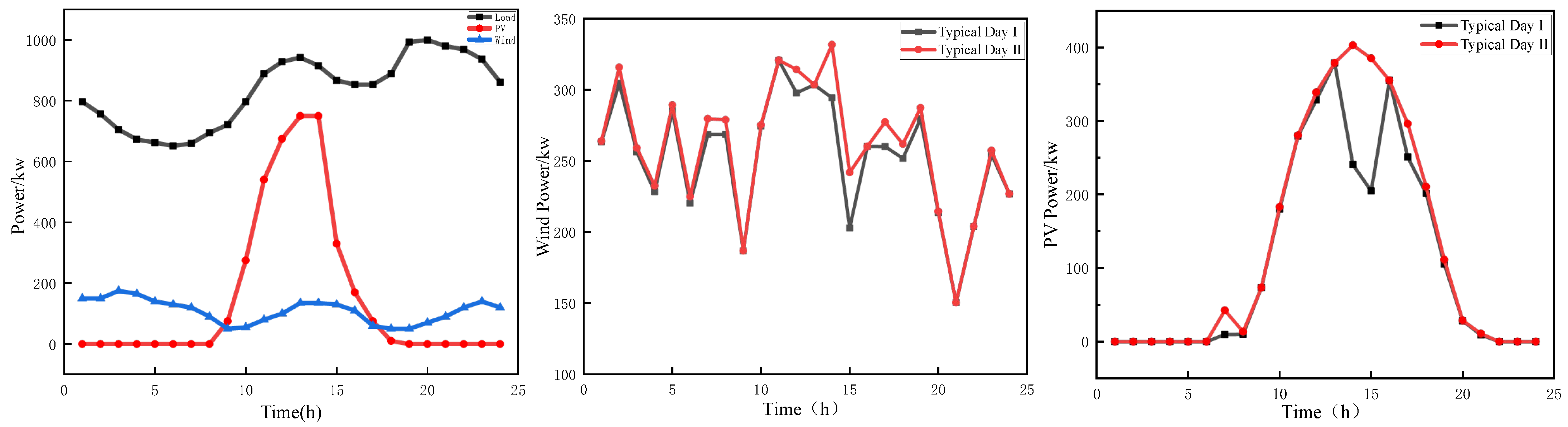
6.1. Data Preparation

Considering the obvious seasonality of power, based on historical data from Zhangbei Wind and Solar Base in China, the sampling interval of the dataset is 1 h, and the state transition process of the daily time cycle is simulated. The K-means clustering algorithm is used to cluster each day into different types of scenarios to characterize the annual power curve, as shown in Figure 6. Typical Day I is at 08:00–09:00 and 12:00–17:00, with large wind speed, and Typical Day II is at 11:00–15:00, with large light intensity. The model is calculated by MATLAB and CPLEX solvers and compared and analyzed using BWO, PSO, GWO, and IBWO, as well as VMD, EMD, and MVMD.
The operational period of the microgrid is set at 20 years. The fundamental parameter values for the energy storage equipment are presented in Table 4. The costs associated with each piece of equipment, along with their unit parameter values, are detailed in Table 5 and Table 6. Additionally, the penalty coefficients and costs for each pollutant are outlined in Table 7, while the time-of-use electricity pricing is provided in Table 8.

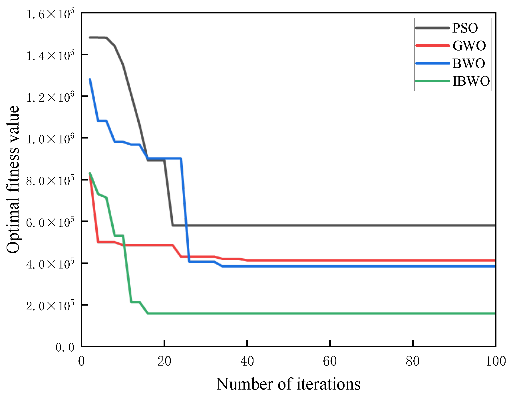
6.2. Comparison and Analysis of IBWO and Other Algorithms

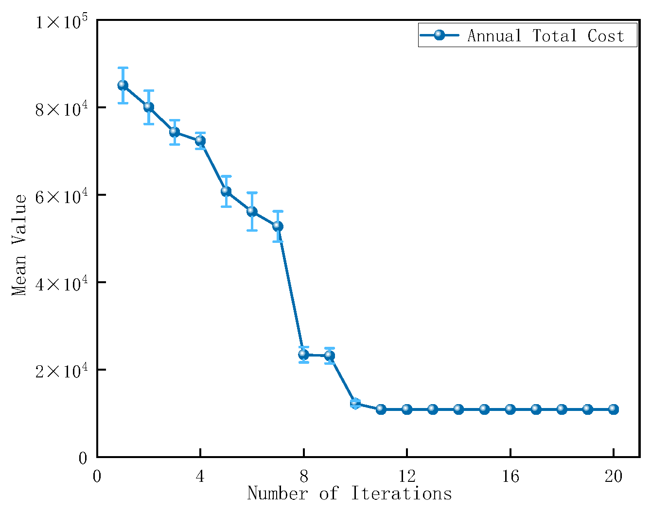
6.2.1. Verifying IBWO Algorithm Performance

From the convergence curve (Figure 7), IBWO demonstrates the fastest convergence, reaching optimal results by the 17th iteration, highlighting its strong optimization efficiency. In the economic analysis (Table 9), the IBWO algorithm effectively reduces total costs, being 21.62%, 7.56%, and 5.91% lower than PSO, GWO, and BWO, respectively. Regarding capacity configuration (Table 10), IBWO achieves higher renewable energy utilization efficiency, with the lowest curtailment rate of just 1.03%, significantly outperforming PSO, BWO, and GWO in terms of curtailment.

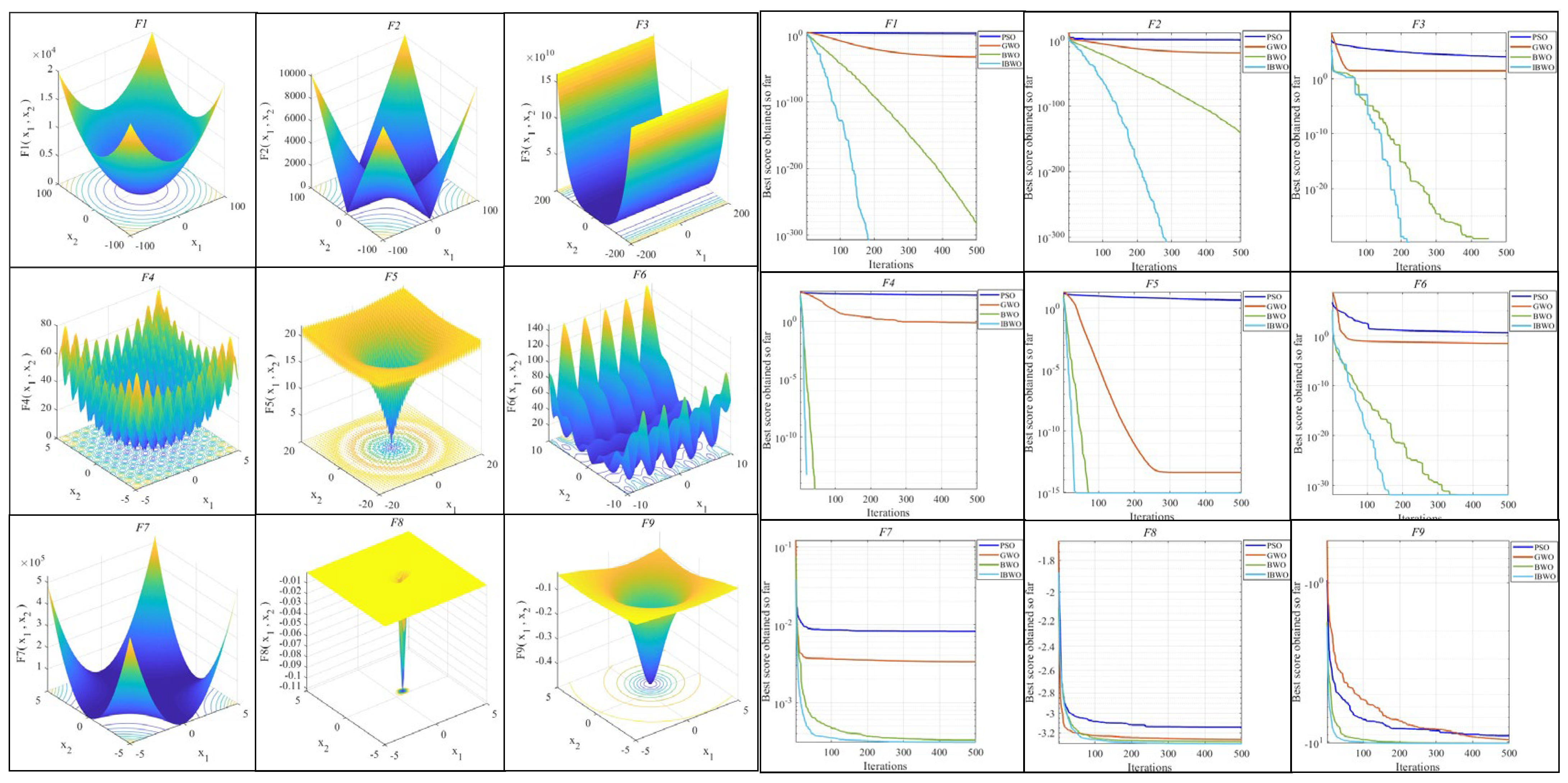
6.2.2. Comparison with Other Test Functions

This paper compares the PSO, GWO, BWO, and IBWO algorithms using nine benchmark test functions. Each algorithm is run for 20 trials, with 500 iterations per trial. The results are shown in Figure 8.
In the test of F1–F3 unimodal continuous functions, the IBWO algorithm demonstrated a rapid convergence speed and a significant reduction in fitness values, in particular, achieving lower fitness values in the early stages of iteration, which is superior to both PSO and GWO. In the tests of the F4–F6 multimodal or complex functions, the PSO performed best at F4, while the IBWO displayed a swift convergence rate at F5. In F6, the competition between IBWO and PSO was fierce, and the final fitness value of IBWO was slightly lower than PSO. For the mixed functions F7–F9, PSO exhibited greater stability in F7, while IBWO and GWO demonstrated faster convergence and BWO slower convergence. In F8, both PSO and IBWO slightly outperformed the other algorithms, while in F9, PSO and IBWO performed similarly; both could quickly converge and had low fitness.
Based on the above, it is evident that the computational complexity of the objective functions F1–F7 increases progressively, while the Improved Beluga Whale Optimization (IBWO) algorithm performs excellently in most optimization problems, particularly in terms of convergence speed and fitness. Specifically, in the more complex hybrid functions F7–F9, both convergence speed and fitness values outperform those of other functions, demonstrating the superiority of the algorithm in handling complex function computations. This also validates the effectiveness of the multistrategy improvement method in enhancing global search capabilities and convergence speed.

6.3. Comparative Analysis of MVMD Performance

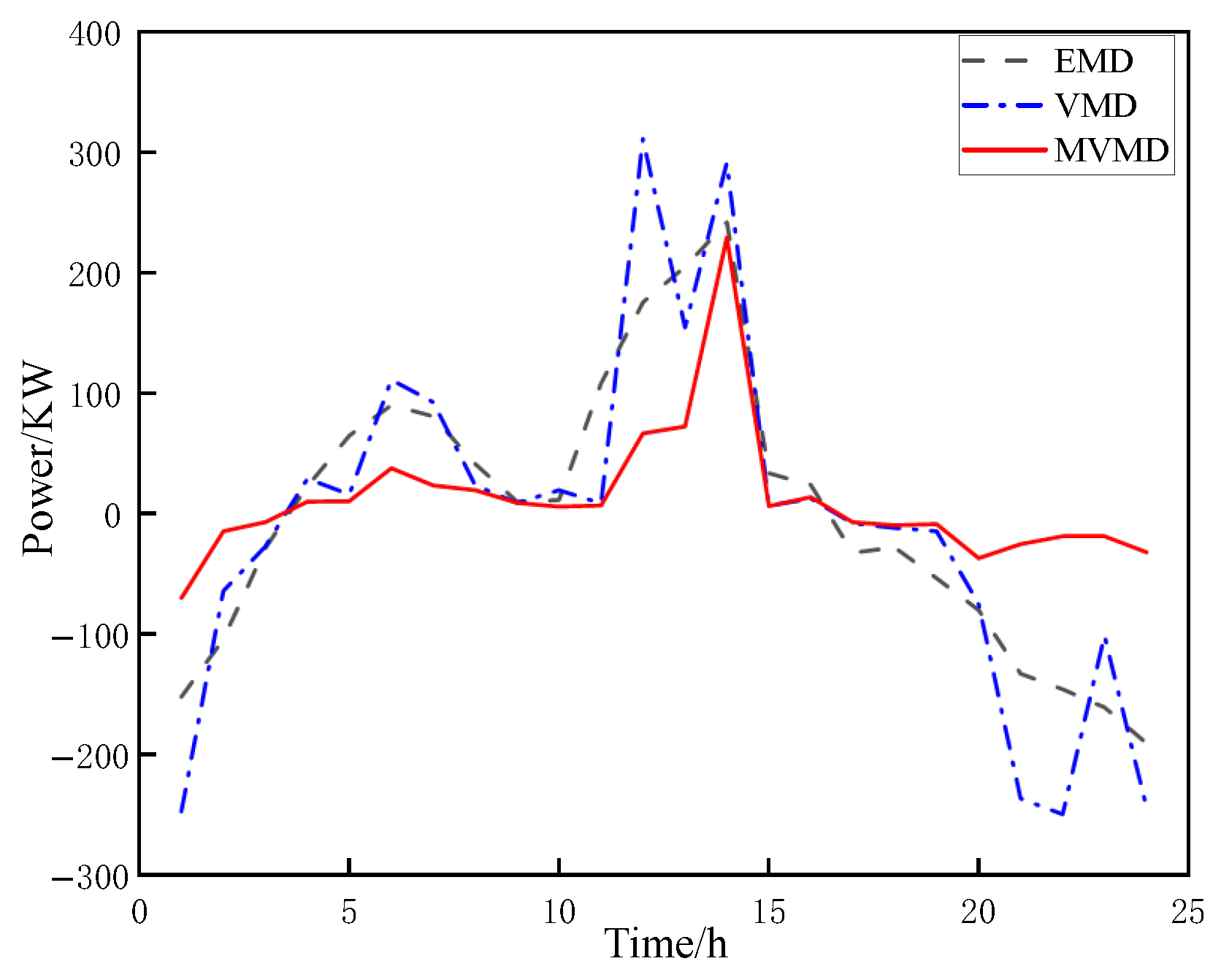
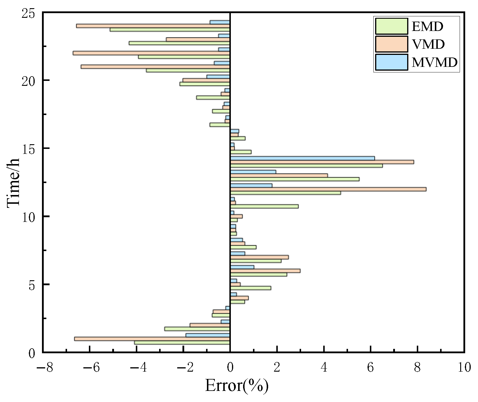
6.3.1. MVMD Compared to Other Modal Decomposition Strategies

Figure 9 illustrates that the power fluctuations following MVMD decomposition are markedly lower than those after EMD and VMD. Figure 10 displays a bar chart that compares the hourly errors between the original power and the decomposed power. The results clearly indicate that MVMD consistently achieves significantly lower decomposition errors compared to both EMD and VMD, demonstrating its superior signal decomposition performance.

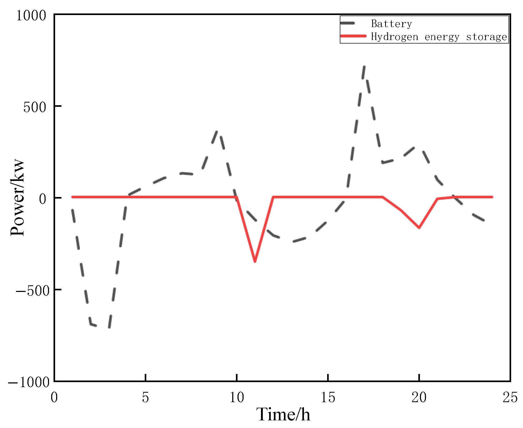
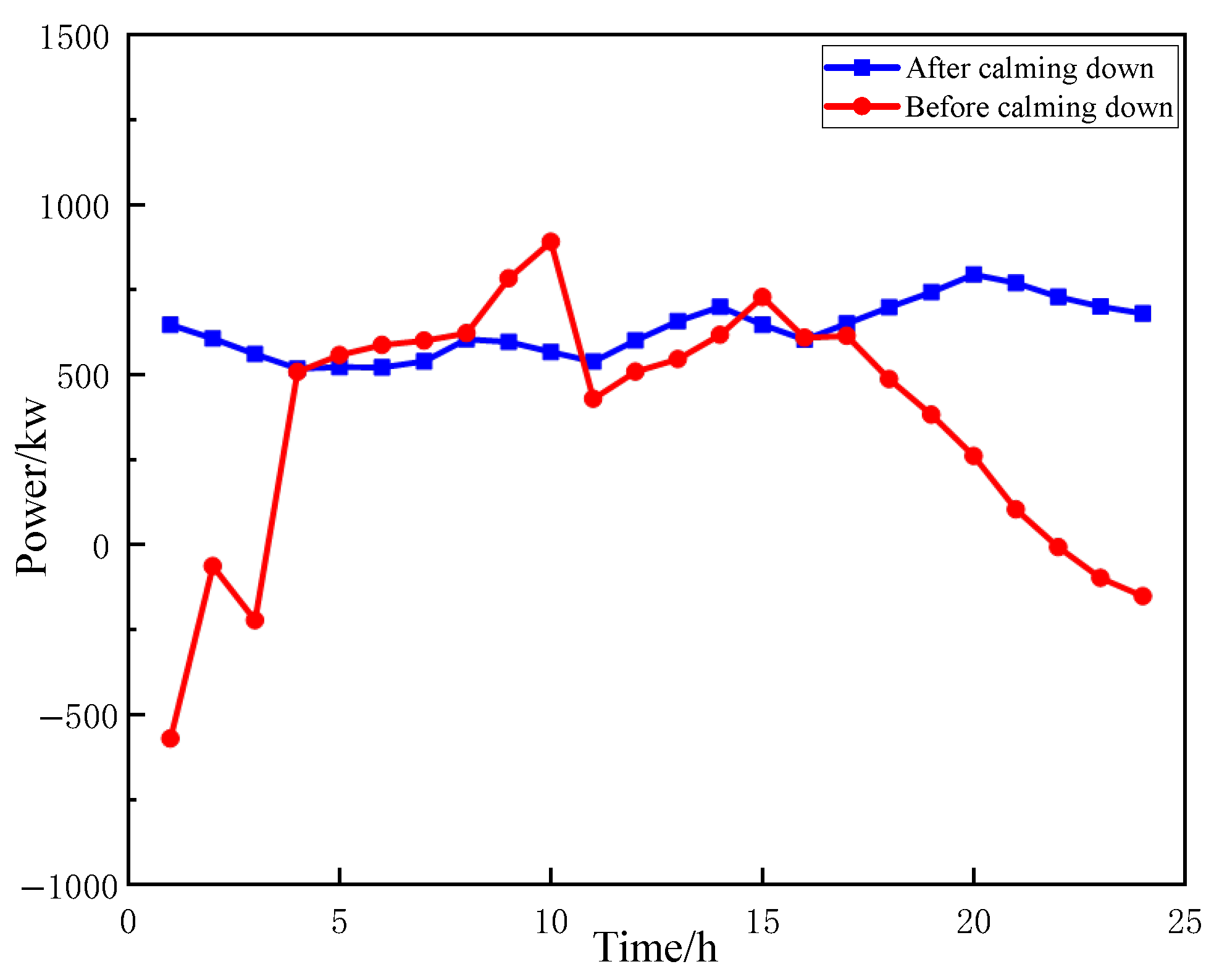
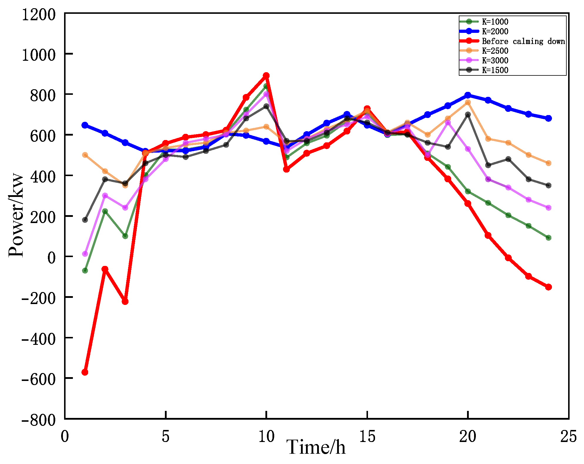
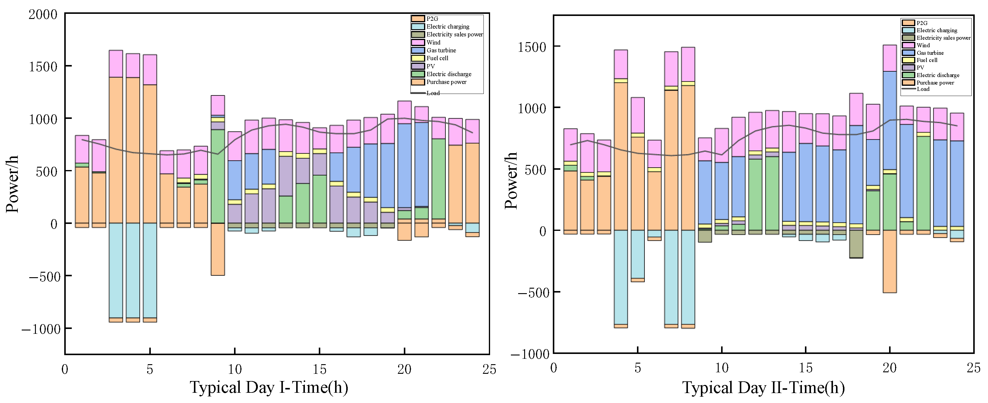
6.3.2. Analysis of Power Fluctuation Smoothing Effect and Power Allocation Results in Hybrid Energy Storage Systems

In photovoltaic–wind hybrid systems, the hybrid energy storage system is essential for compensating the disparity between generated power and grid-connected power, effectively mitigating system fluctuations. The mode decomposition results and configuration outcomes for two typical days are shown in Table 11. Figure 11 illustrates the internal power allocation within the hybrid energy storage system, while Figure 12 compares the power fluctuation levels before and after smoothing. Based on Typical Day II, the impact of different mode numbers on the system’s power fluctuation attenuation effect is investigated by varying the decomposition mode number (K). The values of K are set as 1000, 1500, 2000, 2500, and 3000, with a grid mode number of 2, as shown in Figure 13.
Based on the power generation scenarios of two typical days (Table 11), the MVMD algorithm adaptively determines the number of decomposition modes and grid-connected modes, effectively addressing the issues of over-decomposition or under-decomposition that arise from the subjective mode selection in traditional VMD algorithms.
As illustrated in Figure 11, the battery, characterized by its higher energy density, operates at a lower frequency, with extended charge and discharge durations. In contrast, the hydrogen storage system, recognized for its higher response density, functions at a higher frequency, demonstrating quicker charging and discharging transitions. The power distribution strategy aligns with the charging and discharging characteristics of both the battery and hydrogen storage.
Figure 12 presents a comparison of power fluctuations before and after smoothing. After MVMD decomposition, the grid-connected power curve is significantly smoother, with the maximum power fluctuation decreased to 7.63%, thus meeting grid requirements. This approach effectively captures the overall generation trend of photovoltaic and wind power. Furthermore, the energy storage system absorbs energy during power surges and releases energy during power drops, demonstrating its effectiveness in peak shaving and smoothing power fluctuations.
Figure 13 shows the influence of different modal numbers on the smoothing effect. When the number of modes (K) is set to 2000, the curve exhibits the best performance, indicating an effective attenuation of power fluctuations. If the number of modes is set too low (K = 1000 or K = 1500), the system may fail to adequately decompose the primary characteristics of power fluctuations, resulting in an inability to suppress certain critical fluctuation patterns. Consequently, significant power oscillations may persist, adversely affecting the optimization performance of the energy storage system. On the other hand, if the number of modes is set too high (K = 2500 or K = 3000), the system may undergo excessive decomposition, leading to increased computational complexity. Additionally, some insignificant high-frequency noise components may be mistakenly extracted, introducing unnecessary fluctuations and ultimately reducing the overall effectiveness of power fluctuation suppression.

6.4. Multiscenario Comparison

In various application scenarios, this study utilizes the IBWO algorithm and MVMD algorithm for model computations. It presents configuration schemes for different scenarios (Table 12), capacity configuration results (Table 13), and cost configuration results (Table 14). The single-layer model is solved using the IBWO algorithm. In the dual-layer model, the outer layer employs the IBWO algorithm for capacity configuration, while the inner layer uses the MVMD algorithm for power scheduling.
Scenario 1: Single-Level Optimization Model.
Scenario 2: Bi-Level Optimization Model with Battery Energy Storage.
Scenario 3: Bi-Level Optimization Model with Hydrogen Energy Storage.
Scenario 4: Single-Level Model with Electro-Hydrogen Hybrid Energy Storage.
Scenario 5: Bi-Level Model with Electro-Hydrogen Hybrid Energy Storage.
A comparative analysis of the results across the five scenarios reveals that compared to the single-level hybrid energy storage model, the bi-level model achieves a substantial 27.5% reduction in system costs. Additionally, it significantly decreases energy curtailment, effectively alleviating the pressure on power generation during periods of insufficient wind and solar energy. These findings highlight the bi-level model’s superiority in minimizing configuration costs while enhancing energy utilization efficiency.

6.5. Results and Optimal Capacity Analysis

To visually display the configuration results of the system, a stacked bar chart can be used for visualization. As shown in Figure 14, the power generated by the system (such as wind power and photovoltaic power generation) is represented by positive values, while the power consumed by the system (such as the power load of the base station) is represented by negative values. By reasonably configuring wind power, photovoltaic, and energy storage capacity, the system can dynamically balance energy supply and consumption at different time periods, effectively reduce overall energy consumption, and optimize economy. The results are shown in Table 15.
Table 15 and Figure 14 present the capacity configuration results for various typical days. In comparison to Typical Day I, there is a significant increase in photovoltaic and wind power generation on Typical Day II, which leads to a greater allocation of hydrogen energy storage. This highlights the system’s adaptive strategy of increasing hydrogen storage capacity during periods of abundant wind and solar resources to efficiently store and utilize surplus electricity. Conversely, when wind and solar resources are limited, the system adopts a differentiated response mechanism: batteries are utilized for rapid response to high-frequency, short-term demands, while hydrogen storage caters to low-frequency, long-duration requirements. This approach effectively mitigates power fluctuations caused by insufficient wind and solar generation during high-load demand periods. The model demonstrates how the microgrid dynamically adjusts the configuration of energy storage and generation systems based on power fluctuations under varying wind and solar resource conditions. This ensures both the stability of the power supply and the economic efficiency of the system.
Figure 15 shows the error situation of the optimization results. At the early stages of iteration, the number of iterations is insufficient, leading to noticeable fluctuations in the data, indicating that the model has not yet converged. As the number of iterations increases, the error gradually decreases, suggesting an improvement in data stability and a progressive convergence of the results. In the final stage, the error bars nearly disappear, signifying that the model or experiment has reached a stable state.

6.6. Sensitivity Testing

With technological advancements and increased productivity, the utilization of distributed generation has risen, while energy storage costs continue to decline. As a result, conducting a sensitivity analysis on key system parameters has become an essential method for evaluating the system’s response to changes in external conditions. Assuming that climate conditions and load demand remain constant, this analysis investigates the impact of variations in energy storage costs on system configuration and operational strategies, as illustrated in Table 16.
Table 16 presents the sensitivity analysis of energy storage cost on the system. As the cost of energy storage devices continues to decrease, the allocation of hydrogen storage capacity significantly increases, while the rate of growth in the system’s total cost decelerates. This trend not only creates potential for system expansion during the initial phases of development but also improves the efficiency of renewable energy utilization and enhances the microgrid’s stability in handling seasonal fluctuations. Given the ongoing advancements in low-carbon development and technology, the future prospects for hydrogen storage appear highly promising.

7. Conclusions

This paper presents a solar–wind-based electro-hydrogen hybrid energy storage bi-level capacity optimization model designed to balance economic efficiency and stability within microgrids, with the abandonment rate serving as an evaluation metric. The outer layer employs a multistrategy Improved Beluga Whale Optimization (IBWO) algorithm for energy storage capacity planning, achieving cost reductions of 21.62%, 7.56%, and 5.91% compared to PSO, GWO, and BWO, respectively. The inner layer utilizes an MVMD algorithm for power output scheduling. Compared to traditional VMD and EMD algorithms, the MVMD algorithm significantly reduces power fluctuations and hourly errors, smoothing maximum power fluctuations to 7.63% and demonstrating excellent performance in peak shaving and fluctuation mitigation. Overall, the dual-layer optimization model reduces the annual comprehensive cost by 27.5% compared to the single-layer optimization model. It dynamically adjusts the energy storage and generation system configurations based on varying solar and wind resources, significantly enhancing the economic efficiency and stability of microgrid power supply. However, this study primarily focuses on optimizing wind and photovoltaic power scheduling based on historical data without fully accounting for the stochastic impacts of extreme weather, climate change, and other uncertainties. Additionally, the integration of market mechanisms remains insufficient, as it does not thoroughly consider the competitive electricity market environment and the influence of ancillary service markets on energy storage optimization strategies.
In the future, incorporating electricity market mechanisms into scheduling strategies, along with the integration of more accurate probabilistic forecasting models or reinforcement learning techniques, could enhance the model’s adaptability to complex and dynamic environments. Additionally, regulatory authorities can establish more detailed operational standards for energy storage systems and promote the development of standardized data-sharing platforms. This would facilitate the coordinated optimization among renewable energy generation enterprises, energy storage operators, and grid companies, thereby improving the overall accuracy of system dispatch and enhancing its resilience to risks.

Author Contributions

Q.X.: writing—review and editing, writing—original draft, formal analysis, data curation, conceptualization. S.L.: writing—review and editing, data curation, formal analysis. D.Q.: methodology. Y.L. (Yang Long): data curation. Q.L.: conceptualization. X.Y.: conceptualization. Y.L. (Yunxiang Li): conceptualization. K.Q.: funding acquisition. All authors have read and agreed to the published version of the manuscript.

Funding

This work was supported by the National Natural Science Foundation of China [grant numbers 62365009] and Hubei Provincial Department of Education Youth and Middle-Aged Talent Project [grant number T2021013].

Data Availability Statement

Data will be made available on request.

Conflicts of Interest

The authors declare that they have no known competing financial interests or personal relationships that could have appeared to influence the work reported in this paper.

References

  1. Gan, C.K.; Tan, Y.C.; Wong, K.H. Microgrid and its applications: A review. J. Clean. Prod. 2018, 186, 773–783. [Google Scholar]
  2. Mohsin, N.; Jha, S.K. Optimal design of microgrids with hybrid energy storage systems. Energies 2019, 12, 2708. [Google Scholar]
  3. Liang, Y.; Chen, W.; Zhang, Y. A survey on swarm intelligence algorithms. J. Comput. Sci. 2019, 30, 239–249. [Google Scholar] [CrossRef]
  4. Chen, Y.; Zhao, X.; Yuan, J. Swarm Intelligence Algorithms for Portfolio Optimization Problems: Overview and Recent Advances. Mob. Inf. Syst. 2022, 2022, 4241049. [Google Scholar] [CrossRef]
  5. Feng, Z.; Liu, H.; Zhang, Y. An adaptive particle swarm optimization algorithm based on chaotic mapping. Appl. Sci. 2020, 10, 5637. [Google Scholar] [CrossRef]
  6. Zhou, Y.; Yang, J.; Guo, C. Application of improved particle swarm optimization in power system optimization. Energy Rep. 2021, 7, 251–258. [Google Scholar] [CrossRef]
  7. Li, X.; Zhang, J.; He, Y.; Zhang, Y.; Liu, Y.; Yan, K. Multi-objective optimization scheduling of microgrids based on improved particle swarm optimization algorithm. Electr. Power Sci. Eng. 2021, 37, 1–10. [Google Scholar]
  8. Liu, C.; Sun, Z. Green flexible production and intelligent factory building structure design based on improved ant colony algorithm. Therm. Sci. Eng. Prog. 2024, 53, 102753. [Google Scholar] [CrossRef]
  9. Fan, H.; Wu, H.; Li, S.; Han, S.; Ren, J.; Huang, S.; Zou, H. Optimal Scheduling Method of Combined Wind–Photovoltaic–Pumped Storage System Based on Improved Bat Algorithm. Processes 2025, 13, 101. [Google Scholar] [CrossRef]
  10. Huang, Z.; Bei, L.; Wang, B.; Xu, L. Capacity optimization configuration for a park-level hybrid energy storage system based on an improved cuckoo algorithm. Processes 2024, 12, 718. [Google Scholar] [CrossRef]
  11. Wang, S.; Zhang, L. White whale optimization algorithm for optimal sizing of energy storage systems in microgrids. Renew. Energy 2020, 148, 1347–1357. [Google Scholar]
  12. Zhou, X.; Li, J. Application of white whale optimization algorithm in renewable energy systems. Renew. Energy 2021, 45, 57–69. [Google Scholar]
  13. Zhao, N.; Zhang, L.; Li, D.; Huang, W.; Xie, W.; Yang, Y. Capacity optimization configuration method for wind-solar-hydrogen-storage microgrids based on improved honey badger algorithm. J. Electr. Eng. 2025, 20, 338–351. [Google Scholar]
  14. Liao, X.; Lei, R.; Ouyang, S.; Huang, W. Capacity Optimization Allocation of Multi-Energy-Coupled Integrated Energy System Based on Energy Storage Priority Strategy. Energies 2024, 17, 5261. [Google Scholar] [CrossRef]
  15. Liu, Y.J.; Wang, J.F.; Liu, K.S. Dynamic modal analysis for power fluctuation in microgrid systems. Energy Rep. 2020, 5, 567–573. [Google Scholar]
  16. Farhangi, H.R. Control strategies for energy management in microgrids using modal decomposition. Renew. Energy 2021, 163, 511–520. [Google Scholar]
  17. Zhang, Y.; Li, M.; Wang, L. A comprehensive review of modal decomposition techniques: Emd, vmd, and their applications. IEEE Access 2020, 8, 175054–175075. [Google Scholar]
  18. Lei, S.; He, Y.; Zhang, J.; Deng, K. Optimal configuration of hybrid energy storage capacity in a microgrid based on variational mode decomposition. Energies 2023, 16, 4307. [Google Scholar] [CrossRef]
  19. Liu, H.; Zhang, W.; Chen, J. Power oscillation damping using empirical mode decomposition and adaptive control. IEEE Trans. Power Syst. 2021, 36, 1534–1543. [Google Scholar]
  20. Feng, C.; Wang, Y.; Zhang, J. Multiscale variational mode decomposition for fault detection in microgrids. IEEE Access 2020, 8, 129425–129436. [Google Scholar]
  21. Zhang, X.; Liu, Q.; Wang, Y. Application of multiscale variational mode decomposition in microgrid stability analysis. Renew. Energy 2021, 167, 227–237. [Google Scholar]
  22. Li, X.; Zhang, H. Application of mvmd in power smoothing of microgrids with renewable energy integration. IEEE Trans. Sustain. Energy 2021, 12, 1590–1599. [Google Scholar]
  23. Zhang, Y.; Chen, L.; Wang, J. Comparison and improvement of mvmd and vmd for power smoothing in microgrids. Electr. Power Syst. Res. 2020, 189, 106742. [Google Scholar]
  24. Liu, Y.; Zhao, Q. Case study of mvmd in power output stabilization for photovoltaic integrated microgrids. J. Renew. Sustain. Energy 2023, 15, 043001. [Google Scholar]
  25. El-Sharkawy, M.M.; Shakib, A.S. Modal decomposition for energy storage optimization in microgrids. J. Energy Storage 2022, 48, 103501. [Google Scholar]
  26. Liu, Y.; Zhang, X.; Li, T. Energy storage systems and their applications in microgrids: A review. Renew. Sustain. Energy Rev. 2020, 121, 109738. [Google Scholar]
  27. Zhou, Y.; Liu, F. The role of flywheel energy storage in microgrid operations: A review. Renew. Sustain. Energy Rev. 2019, 109, 109–120. [Google Scholar]
  28. Yang, Y.; Zhang, X.; Chen, J. Performance analysis of lithium-ion batteries in microgrids: A case study. J. Energy Storage 2020, 28, 101198. [Google Scholar]
  29. Gao, H.; Zhang, Z. Optimal sizing and control of supercapacitors in microgrid applications. IEEE Trans. Power Electron. 2022, 37, 1394–1403. [Google Scholar]
  30. Sutikno, T.; Arsadiando, W.; Wangsupaphol, A.; Yudhana, A.; Facta, M. A review of recent advances on hybrid energy storage system for solar photovoltaics power generation. IEEE Access 2022, 10, 42346–42359. [Google Scholar]
  31. Zheng, Y.; Wang, J.; Zhou, L. Energy management strategies for hybrid energy storage systems in microgrids: A comprehensive review. Renew. Sustain. Energy Rev. 2019, 107, 189–205. [Google Scholar]
  32. Krishan, O.; Suhag, S. A novel control strategy for a hybrid energy storage system in a grid-independent hybrid renewable energy system. Int. Trans. Electr. Energy Syst. 2020, 30, e12262. [Google Scholar] [CrossRef]
  33. Jiang, S.; Wang, Q.; Zhang, Y. Coordinated control strategy of hybrid energy storage system for microgrids. IEEE Trans. Power Syst. 2020, 35, 1002–1013. [Google Scholar]
  34. Tang, Y.; Xun, Q.; Liserre, M.; Yang, H. Energy management of electric-hydrogen hybrid energy storage systems in photovoltaic microgrids. Int. J. Hydrogen Energy 2024, 80, 1–10. [Google Scholar]
  35. Li, J.; Xiao, Y.; Lu, S. Optimal configuration of multi microgrid electric hydrogen hybrid energy storage capacity based on distributed robustness. J. Energy Storage 2024, 76, 109762. [Google Scholar] [CrossRef]
  36. Liu, S.; Wu, J.; Xu, Y. A review of hybrid energy storage systems in microgrid applications. Appl. Energy 2020, 261, 114364. [Google Scholar]
  37. Liu, Y.; Chen, G. Optimization of hybrid energy storage systems combining battery and hydrogen storage for renewable energy applications. Appl. Energy 2021, 283, 116369. [Google Scholar]
  38. Zhong, C.; Li, G.; Meng, Z. Beluga whale optimization: A novel nature-inspired metaheuristic algorithm. Knowl.-Based Syst. 2022, 251, 109215. [Google Scholar]
Figure 1. Microgrid model structure diagram.
Energies 18 01777 g001
Figure 2. Bi-level optimization model diagram.
Energies 18 01777 g002
Figure 3. Flowchart of microgrid operation strategy.
Energies 18 01777 g003
Figure 4. Program flowchart of the IBWO algorithm.
Energies 18 01777 g004
Figure 5. Flowchart of MVMD algorithm program.
Energies 18 01777 g005
Figure 6. Extracted photovoltaic, wind power, load power data, and power data of two typical days.
Energies 18 01777 g006
Figure 7. Optimal results of PSO, GWO, BWO, and IBWO.
Energies 18 01777 g007
Figure 8. Optimal results of other test functions and PSO, GWO, BWO, and IBWO.
Energies 18 01777 g008
Figure 9. Comparison of EMD, VMD, and MVMD.
Energies 18 01777 g009
Figure 10. Comparison of EMD, VMD, and MVMD errors.
Energies 18 01777 g010
Figure 11. Internal power allocation of the hybrid energy storage system.
Energies 18 01777 g011
Figure 12. Changes in grid-connected power fluctuation rate before and after smoothing.
Energies 18 01777 g012
Figure 13. The influence of different modal numbers on the smoothing effect.
Energies 18 01777 g013
Figure 14. Capacity configuration results for Typical Day I and Typical Day II.
Energies 18 01777 g014
Figure 15. Error analysis of optimization results.
Energies 18 01777 g015
Table 1. Comparison of existing methods.
TypeMethodAdvantageLimitationReferences
AlgorithmPSOFast convergence speed and strong adaptabilityLocal convergence, limited accuracy[5,6,7]
ACOSlightly stronger global searchSlow convergence speed[8]
BASlightly stronger global searchLocal convergence, slow convergence speed[9]
BWOStrong global exploration ability and fast convergence speedNeed to finely adjust parameters[11,12]
IBWOSuperior stability and convergence speed, suitable for high uncertainty systemsMore complex calculations-
Mode
decomposition
EMDHigh decomposition accuracyNeed to set the number of modes reasonably[18]
VMDHigh precision, capable of processing complex signalsReasonably set the number of modes[19]
MVMDProcessing multidimensional signals with high accuracy and adaptive adjustment of modal numbersThe model complexity is higher and the calculation is more complex[20,21,22,23,24]
ModelSingle levelSimple and fast calculationSingle scope[5,9]
Bi-levelTaking into account multiple objectives, the output solution is more applicableMore complex calculations[10,11]
Table 2. Relevant parameters of the microgrid and their meanings.
ParameterMeaningParameterMeaning
vReal-time wind speed v c i Rated cut-in speed of wind turbine
v c o Rated cut-out speed of wind turbine η e l e Efficiency of electrolytic cell
v r Rated speed of wind turbine P F C D C Fuel cell output power
f p v Power derating coefficient P tan k F C Hydrogen power input to the fuel cell
P S T C Rated power of photovoltaic panel η F C Fuel cell conversion efficiency
G S T C Solar irradiance intensity η s t o r Hydrogen storage efficiency
T a Ambient temperature E tan k t Hydrogen storage tank energy
P Power temperature coefficient P M T t Real power output of gas turbine
GActual irradiance η M T t Operational efficiency of gas turbine
δ Self-discharge rate of the battery C M T . F t Fuel costs of diesel generators
P c Charging power of the battery T S T C Temperature of the solar panel
P d Discharge power of the battery γ m t , k Emission of k-type pollutants produced
E C Rated capacity of the battery S O C t State of charge of the battery
η c Charging efficiency of the battery Δ t Adjacent time intervals
η d Discharge efficiency of the battery E b a t t Battery capacity
TTemperature of the photovoltaic panel surface P M T t Electricity generation of diesel generators
K M T . O M Operation and maintenance cost coefficient of diesel generators C M T . O M t Operation and maintenance costs of diesel generators
P e l e Input electrical power of the electrolytic cell C M T . E N t Pollutant emission control costs of diesel generators
Table 3. Key parameters and their definitions.
ParameterMeaningParameterMeaning
C n Initial construction cost k b u y The unit price of electricity sold
C r Replacement cost k s e l l The unit price of electricity purchased
C g Grid transaction cost P b u y The power purchased
C e Environmental protection cost P s e l l The power sold
C o m Annual operation and maintenance cost N i The number of distributed power sources
β g r i d , r The emissions of pollutant type r C G . E The cost of pollutant treatment
c i r Replacement cost coefficient P g r i d Trading power with the power grid
S O C min Minimum value of battery capacity P M T Gas turbine output power
S O C max Maximum capacity of battery P e l Charging power of electrolytic cell
P c max Maximum charging power of battery P l o a d Load demand power
P d max Maximum discharge power of battery P w t max Maximum output power of the fan
P M T min Minimum output power of gas turbine P w t The output power of the wind turbine
P M T max Maximum output power of gas turbine P F C The discharging power of the fuel cell
P P V max Maximum output power of photovoltaics P P V The output power of the photovoltaic panel
S i n The rated capacity of the i-th energy source P e l max Maximum charging power of electrolytic cell
Y i The life cycle of the i-th energy source P F C max Maximum discharge power of fuel cells
P g ( t ) Grid-connected power value after stabilization P g r i d max Power limit for trading with the power grid
nTypes of distributed power sources P a b Abandoned renewable energy generation
mThe types of distributed energy resources requiring replacement C r The cost coefficient for treating pollutant type r
E tan k max t Upper limit of capacity for hydrogen storage tank P r a t e d Rated installed capacity of power generation system
E tan k min t Lower limit of capacity for hydrogen storage tank P t o Total electricity generation from renewable energy sources
C i n The investment cost coefficient of the i-th energy source P B A T The charging and discharging power of the battery
C i o m The annual operation and maintenance cost coefficient of the i-th energy source P max , i Rated power generation of the i-th energy device
Δ P max Maximum power fluctuation allowed by the system P a c Actual utilization of renewable energy generation
Table 4. Basic parameters.
ParameterValueParameterValue
η e l e 0.95 S O C min 0.1
η F C 0.95 S O C max 0.9
η s t o r 0.95 Y b a t 0.95
Y e l 20 δ 0.01
Y F C 20 η c 0.95
η d 0.95
Table 5. Unit parameters.
ParameterWTPVGas TurbineGrid
Upper power limit (kw)80050010001500
Power lower limit (kw)0001500
Upper limit of climbing power (kw/min)--4001000
Table 6. Equipment cost.
Type of ProjectConstruction
Cost
(CNY/k)
Operation and
Maintenance
Cost
(CNY/kW·year)
Disposal
Cost
(CNY/k)
Service
Life/Year
WT12,00058954020
PV320015014420
Electrolytic tank6360236286.210
Fuel cell300013213520
Hydrogen storage unit3500170157.520
Oxygen storage device320012014420
Gas turbine15007067.520
Table 7. Pollutant emission coefficient and cost.
Pollutant TypeTreatment Cost
/(CNY)/kg
Pollutant Emission Coefficient
WTPVGas TurbineGrid
C O 2 0.02300724889
S O 2 6000.00361.8
N O x 8000.21.6
Table 8. Price of electricity by time period.
ClassificationPeriod of TimeElectricity Price
/(CNY/kWh)
Electricity Sales
/(CNY/kWh)
Peak time period10:00–11:00, 18:00–22:000.93200.72
Ordinary time period08:00–09:00, 12:00–17:000.62130.53
Valley time period01:00–07:00, 23:00–24:000.31070.28
Table 9. Cost of PSO, GWO, BWO, and IBWO.
AlgorithmCost of
Electricity
Purchase
and Sales
Energy
Storage
Cost
Gas
Purchase
Cost
Environmental
Cost
Income
from
Oxygen
Sales
Energy
Abandonment
Value
Total Cost
IBWO2213.5911016880.0816394482.360625917.46131814678105410,869.49468
PSO2273.1326268270.4055434348.431902958.82786974532254513,863.79794
BWO2068.6589425640.4792274633.4319021078.5259264406253711,552.096
GWO2184.592316510.6596134272.663356901.31438634235212511,759.22967
Table 10. Capacity configuration of PSO, GWO, BWO, and IBWO.
AlgorithmP2GFuel CellElectric
Energy
Storage
Hydrogen
Energy
Storage
Gas
Turbine
P2GDiscard
Rate
IBWO80039.81576152718.234571193.051515248001031.03%
PSO90043.02271848589.473684288.804297038002672.67%
BWO120043.02271848459.7164407108.98910418002762.76%
GWO10001118.0022341096.20901164.07920161202792.79%
Table 11. Mode numbers and configuration results for different typical days.
Typical DayDecomposition
Mode Number
Grid-Connected
Mode Number
BatteryHydrogen
Energy
Storage
Total
Cost
Typical Day I150017501808753
Typical Day II20002718936880
Table 12. Configuration schemes for different scenarios.
ScenarioBatteryHydrogen Energy StorageSingle-LevelBi-Level
1
2
3
4
5
Table 13. Scheme configuration results under different scenarios.
ScenarioPVWindP2GFuel CellElectric
Energy
Storage
Hydrogen
Energy
Storage
Gas Turbine
175017500000
275017500120000
37501750003000
475017585050752.1102785
575017580039.81576718.234693.05152750
Table 14. Scheme configuration costs under different scenarios.
ScenarioCost of
Electricity
Purchase
and Sales
Energy
Storage
Cost
Gas
Purchase
Cost
Environmental
Cost
Income
from
Oxygen
Sales
Energy
Abandonment
Value
Total
Cost
120,761.063410805215680201532,396.06341
211,863.4648111,161.1504612560184231,168.56974
36779.1227479498.8135023963.33444677178519,372.26984
43873.7844278084.0964896.2963.334439851161.50814,993.92274
52213.5911016880.0824482.361917.46134678105410,869.49468
Table 15. Typical daily results analysis.
Typical DayPVWindP2GFuel CellElectric
Energy
Storage
Hydrogen
Energy
Storage
Gas
Turbine
Day I40.2978334.6501120032.6456765.2968297.6342800
Day II378.9116320.6967120044.5213902.8892595.1159800
Table 16. Sensitivity analysis of energy storage cost on the system.
Cost Reduction
Coefficient of Energy
Storage Equipment
Electric
Energy
Storage
Hydrogen
Energy
Storage
Hybrid Energy
Storage Cost
Total Cost
5%728.6739068107.00924258744.08688210,652.10479
10%677.8947368102.12494168134.73684213,586.52198
15%812.3125.33746989747.611,321.05408
20%832.6075188.69108189991.2911,524.04507
25%836.7705375190.577992710,041.2464511,662.33361
30%840.9543902223.210,091.4526811,559.70508
Disclaimer/Publisher’s Note: The statements, opinions and data contained in all publications are solely those of the individual author(s) and contributor(s) and not of MDPI and/or the editor(s). MDPI and/or the editor(s) disclaim responsibility for any injury to people or property resulting from any ideas, methods, instructions or products referred to in the content.

