
Implementing a Hybrid Quantum Neural Network for Wind Speed Forecasting: Insights from Quantum Simulator Experiences


Abstract
1. Introduction
1.1. Classification of Existing Works in Wind Speed/Power Forecasting
1.2. Applications of Quantum Computing in Power and Energy Engineering
1.3. Quantum Computer, Quantum/Digital Annealer, and Quantum Simulator
1.4. Insights and Contributions of This Work
- (a)
- Examination of the architectural parameters of the QNN using the Quantum Approximate Optimization Algorithm (QAOA) embedding layer, such as the number of qubits and wires, to enhance accuracy and overcome barren plateaus.
- (b)
- Evaluation of the model’s performance on different computing hardware facilities, including NVIDIA GPU cuDNN, GPU-only, and CPU, to demonstrate the applicability of modern quantum simulators.
- (c)
- Comparison of the performance of the QAOA-based QNN with other quantum embedding and layer circuits, highlighting the advantages of the QAOA-based QNN approach.
- (d)
- Comparison of the performance of different quantum simulation platforms, such as PennyLane and Torchquantum.
2. Background of Quantum Neural Networks
2.1. Qubits and Ansatz
2.2. Variational Quantum Eigensolver (VQE)
2.3. Quantum Approximate Optimization Algorithm (QAOA)
- (a)
- Creating a PQC called the Mixing Circuit, which transforms the initial state into a list of candidate solutions. The parameters of this circuit are part of the objective function to be optimized.
- (b)
- Creating a PQC called the Phase Circuit, which adjusts the circuit’s parameters to increase the expected value of the objective function at each iteration.
3. Methodology
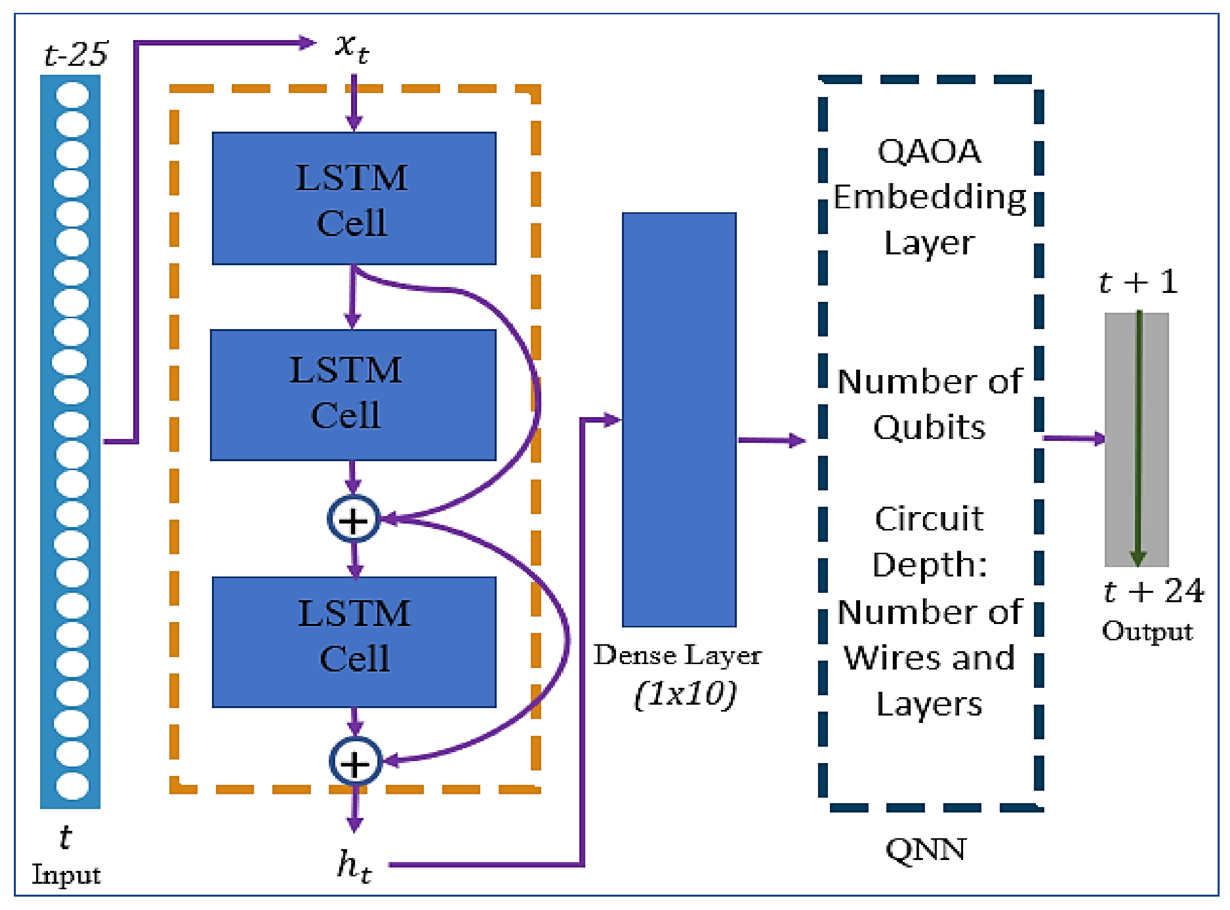
3.1. Residual LSTM
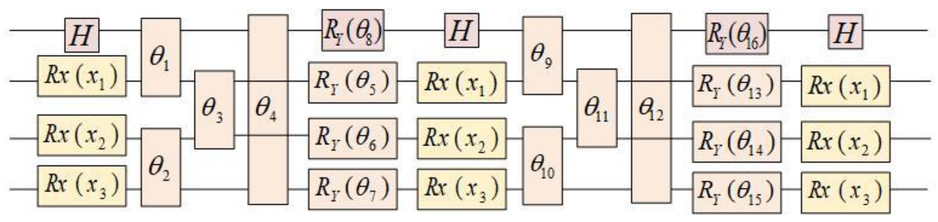
3.2. Quantum Neural Network (QNN)
3.3. Implementation of QNN
3.4. Quantum Simulator
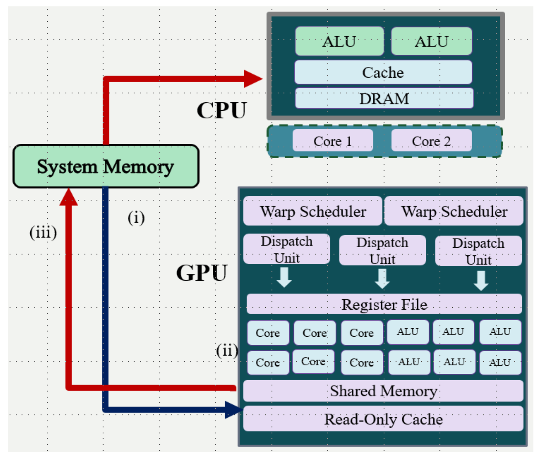
3.5. Compute Unified Device Architecture (CUDA)
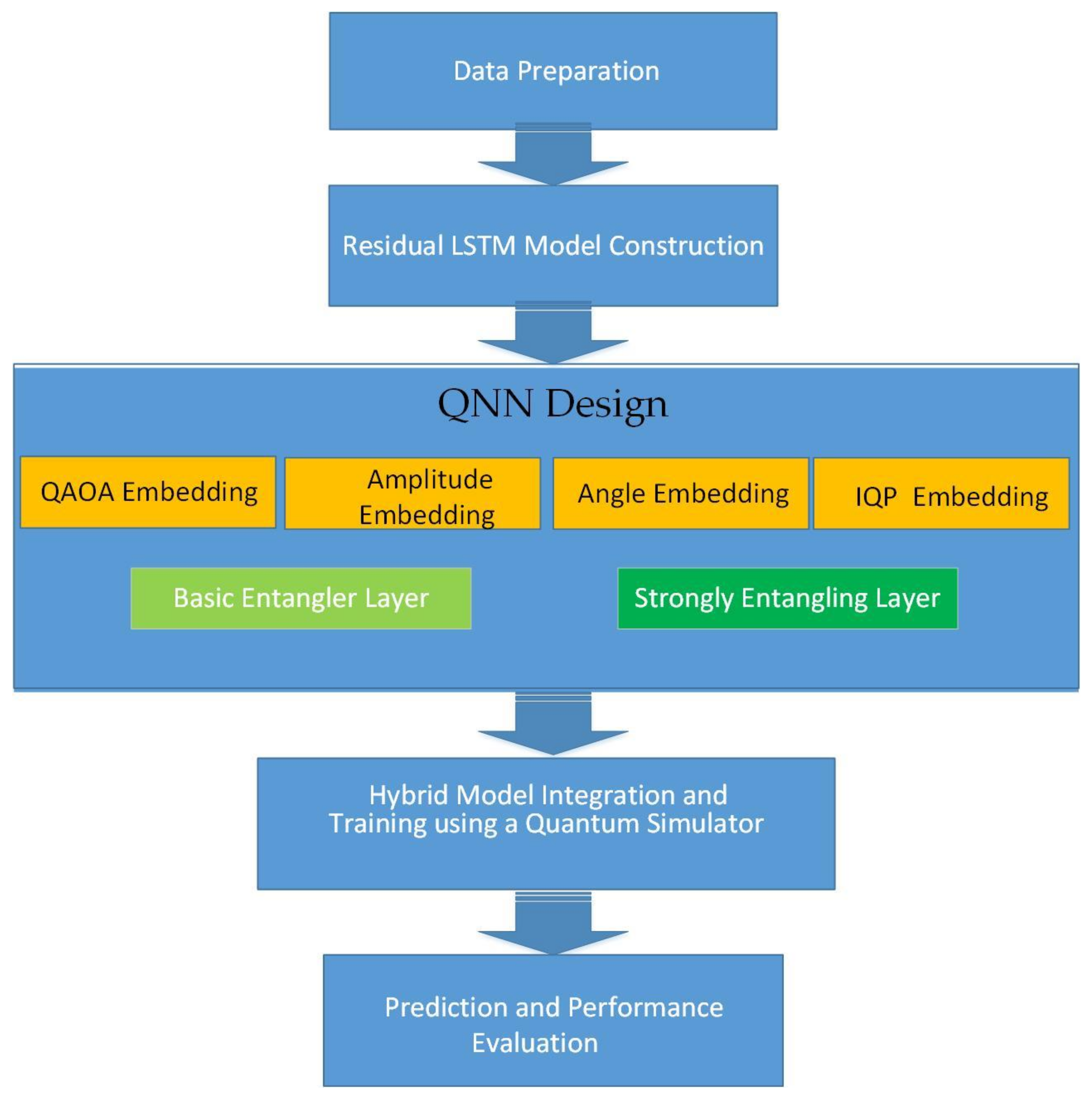
3.6. Solution Steps for Proposed Methodology
- Step 1: Data Preparation
- Step 2: Residual LSTM Model Construction
- Step 3: Quantum Neural Network (QNN) Design
- Step 4: Hybrid Model Integration and Training using a Quantum Simulator
- Step 5: Prediction and Performance Evaluation
4. Results
4.1. Comparative Studies of Runtime
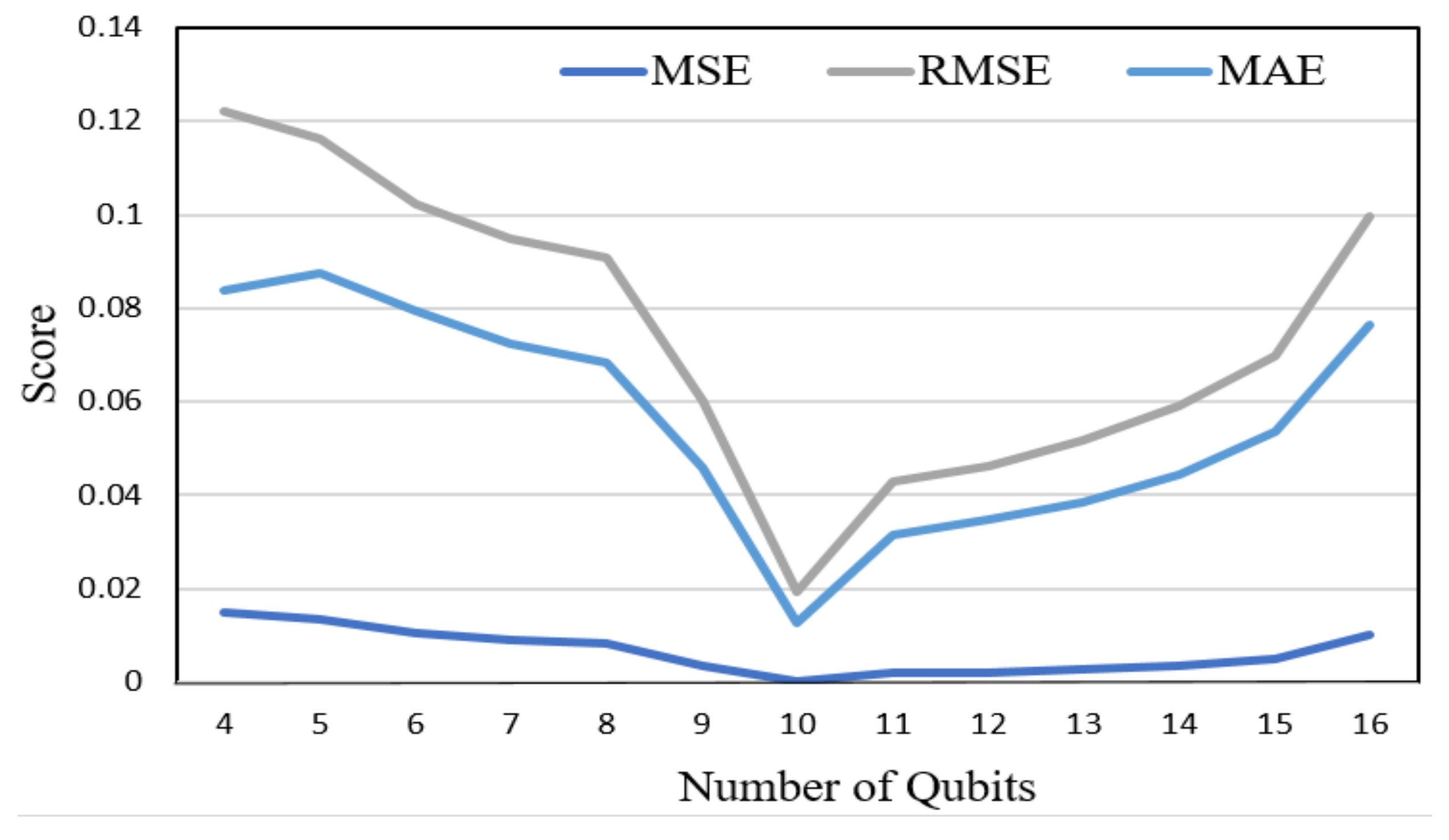
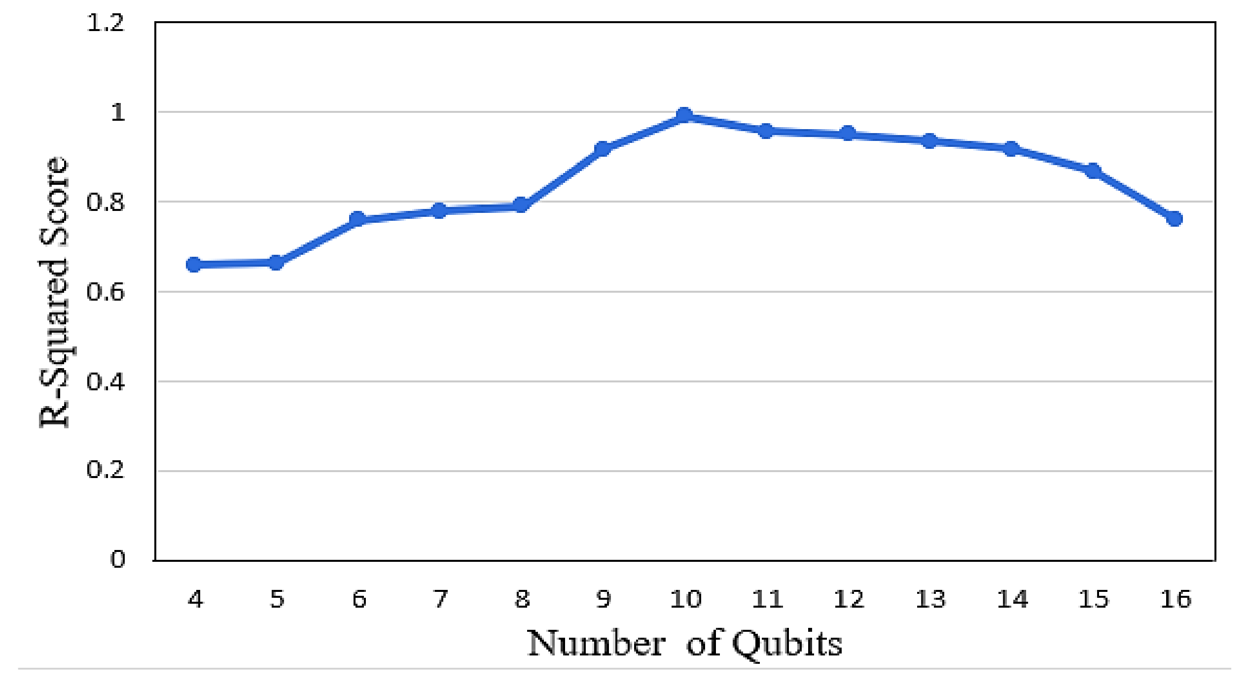
4.2. Comparative Studies of Accuracy
4.3. Comparative Studies of Accuracy with Other QNN and Traditional Methods
4.4. Comparative Studies of Accuracy and Runtime Using Different Quantum Simulators
5. Conclusions
- (a)
- Hybrid quantum algorithms, such as QAOA, offer the combined benefits of classical and quantum algorithms, resulting in significantly improved forecasting accuracy.
- (b)
- QNNs based on the QAOA layer provide more accurate predictions due to the gradient computation support for both features and weights, facilitating better optimization.
- (c)
- The selection of the appropriate number of wires and qubits in the QNN layer is crucial, as it can lead to favorable evaluation metrics and reduced training time.
- (d)
- Quantum simulators utilizing CUDA-based GPUs serve as a suitable hardware platform for studying quantum algorithms, especially in cases where general-purpose quantum computers are not widely available. The training time required by CUDA-based GPUs is found to be the shortest, followed by GPUs, and then CPUs.
Author Contributions
Funding
Data Availability Statement
Conflicts of Interest
Appendix A
- Expectation Value in QAOA
- 2.
- Parameter-Shift Rule for QAOA Gradient
Appendix B
References
- Zhao, Z.; Luo, X.; Xie, J.; Gong, S.; Guo, J.; Ni, Q. Decentralized grid-forming control strategy and dynamic characteristics analysis of high-penetration wind power microgrids. IEEE Trans. Sustain. Energy 2022, 13, 2211–2225. [Google Scholar] [CrossRef]
- Akhtar, I.; Kirmani, S.; Jameel, M. Reliability assessment of power system considering the impact of renewable energy sources integration into grid with advanced intelligent strategies. IEEE Access 2021, 9, 32485–32497. [Google Scholar] [CrossRef]
- Ali, S.W.; Sadiq, M.; Terriche, Y.; Ahmad, S.; Naqvi, R.; Quang, L.; Hoang, N.; Mutarraf, M.U. Offshore wind farm-grid integration: A review on infrastructure, challenges, and grid solutions. IEEE Access 2021, 9, 102811–102827. [Google Scholar] [CrossRef]
- Yousuf, M.U.; Al-Bahadly, I.; Avci, E. Current perspective on the accuracy of deterministic wind speed and power forecasting. IEEE Access 2019, 7, 159547–159564. [Google Scholar] [CrossRef]
- Lipu, M.S.H.; Miah, M.S.; Hannan, M.A.; Hussain, A.; Sarker, M.R.; Ayob, A. Artificial intelligence based hybrid forecasting approaches for wind power generation: Progress, challenges and prospects. IEEE Access 2021, 9, 102460–102489. [Google Scholar] [CrossRef]
- Chen, Y.; Hu, X.; Zhang, L. A review of ultra-short-term forecasting of wind power based on data decomposition-forecasting technology combination model. Energy Rep. 2022, 8, 14200–14219. [Google Scholar] [CrossRef]
- Qian, Z.; Pei, Y.; Zareipour, H.; Chen, N. A review and discussion of decomposition-based hybrid models for wind energy forecasting applications. Appl. Energy 2019, 235, 939–953. [Google Scholar] [CrossRef]
- Vikash, K.S.; Rajesh, K.; Ameena, S.A.; Sujil, A.; Ehsan, H.F. Learning based short term wind speed forecasting models for smart grid applications: An extensive review and case study. Electr. Power Syst. Res. 2023, 222, 109502. [Google Scholar] [CrossRef]
- Liu, H.; Chen, C.; Lv, X.; Wu, X.; Liu, M. Deterministic wind energy forecasting: A review of intelligent predictors and auxiliary methods. Energy Convers. Manag. 2019, 195, 328–345. [Google Scholar] [CrossRef]
- Wang, Y.; Zou, R.; Liu, F.; Zhang, L.; Liu, Q. A review of wind speed and wind power forecasting with deep neural networks. Appl. Energy 2021, 304, 117766. [Google Scholar] [CrossRef]
- Daley, A.J.; Bloch, I.; Kokail, C.; Flannigan, S.; Pearson, N.; Troyer, M.; Zoller, P. Practical quantum advantage in quantum simulation. Nature 2022, 607, 667–676. [Google Scholar] [CrossRef] [PubMed]
- Ajagekar, A.; You, F. Quantum computing for energy systems optimization: Challenges and opportunities. Energy 2019, 179, 76–89. [Google Scholar] [CrossRef]
- Deng, Z.; Wang, X.; Dong, B. Quantum computing for future real-time building HVAC controls. Appl. Energy 2023, 334, 120621. [Google Scholar] [CrossRef]
- Ajagekar, A.; You, F. Quantum computing based hybrid deep learning for fault diagnosis in electrical power systems. Appl. Energy 2021, 303, 117628. [Google Scholar] [CrossRef]
- Zhou, Y.; Zhang, P. Noise-resilient quantum machine learning for stability assessment of power systems. IEEE Trans. Power Syst. 2023, 38, 475–487. [Google Scholar] [CrossRef]
- Feng, F.; Zhang, P.; Bragin, M.A.; Zhou, Y. Novel resolution of unit commitment problems through quantum surrogate Lagrangian relaxation. IEEE Trans. Power Syst. 2023, 38, 2460–2471. [Google Scholar] [CrossRef]
- Nikmehr, N.; Zhang, P.; Bragin, M.A. Quantum distributed unit commitment: An application in microgrids. IEEE Trans. Power Syst. 2022, 37, 3592–3603. [Google Scholar] [CrossRef]
- Feng, F.; Zhou, Y.; Zhang, P. Quantum power flow. IEEE Trans. Power Syst. 2021, 36, 3810–3812. [Google Scholar] [CrossRef]
- Nikmehr, N.; Zhang, P. Quantum-inspired power system reliability assessment. IEEE Trans. Power Syst. 2023, 38, 3476–3490. [Google Scholar] [CrossRef]
- Hong, Y.Y.; Santos, J.B.D. Day-ahead spatiotemporal wind speed forecasting based on a hybrid model of quantum and residual long short-term memory optimized by particle swarm algorithm. IEEE Syst. J. 2023, 17, 6081–6092. [Google Scholar] [CrossRef]
- Ajagekar, A.; You, F. Quantum computing and quantum artificial intelligence for renewable and sustainable energy: A emerging prospect towards climate neutrality. Renew. Sustain. Energy Rev. 2022, 165, 112493. [Google Scholar] [CrossRef]
- Kusyk, J.; Saeed, S.M.; Uyar, M.U. Survey on quantum circuit compilation for noisy intermediate-scale quantum computers: Artificial intelligence to heuristics. IEEE Trans. Quantum 2021, 2, 2501616. [Google Scholar] [CrossRef]
- Ji, X.; Wang, B.; Hu, F.; Wang, C.; Zhang, H. New advanced computing architecture for cryptography design and analysis by D-Wave quantum annealer. Tsinghua Sci. Technol. 2022, 27, 751–759. [Google Scholar] [CrossRef]
- Maruo, A.; Soeda, T.; Igarashi, H. Topology optimization of electromagnetic devices using digital annealer. IEEE Trans. Magn. 2022, 58, 7001504. [Google Scholar] [CrossRef]
- Available online: https://docs.pennylane.ai/en/stable/development/guide/documentation.html (accessed on 13 October 2022).
- Willsch, D.; Willsch, M.; Jin, F.; Michielsen, K.; Raedt, H.D. GPU-accelerated simulations of quantum annealing and the quantum approximate optimization algorithm. Comput. Phys. Commun. 2022, 278, 108411. [Google Scholar] [CrossRef]
- Zhou, L.; Wang, S.T.; Choi, S.; Pichler, H.; Lukin, M.D. Quantum approximate optimization algorithm: Performance, mechanism, and implementation on near-term devices. Phys. Rev. X 2022, 10, 021067. [Google Scholar] [CrossRef]
- Tilly, J.; Chen, H.; Cao, S.; Picozzi, D.; Setia, K.; Li, Y.; Grant, E.; Wossnig, L.; Rungger, I.; Booth, G.H.; et al. The variational quantum eigensolver: A review of methods and best practices. Phys. Rep. 2022, 986, 1–128. [Google Scholar] [CrossRef]
- Choi, J.; Kim, J. A tutorial on quantum approximate optimization algorithm (QAOA): Fundamentals and applications. In Proceedings of the 2019 International Conference on Information and Communication Technology Convergence, Jeju, Republic of Korea, 16–18 October 2019. [Google Scholar] [CrossRef]
- Available online: https://docs.pennylane.ai/en/stable/code/api/pennylane.QAOAEmbedding.html (accessed on 20 October 2022).
- Kim, J.; El-Khamy, M.; Lee, J. Residual LSTM: Design of a deep recurrent architecture for distant speech recognition. arXiv 2017, arXiv:1701.03360. [Google Scholar] [CrossRef]
- Incudini, M.; Grossi, M.; Mandarino, A.; Vallecorsa, S.; Pierro, A.D.; Windridge, D. The quantum path kernel: A generalized quantum neural tangent kernel for deep quantum machine learning. arXiv 2022, arXiv:2212.11826. [Google Scholar] [CrossRef]
- Available online: https://pennylane.ai/devices/lightning-qubit (accessed on 20 October 2022).
- Nikolic, G.S.; Dimitrijevic, B.R.; Nikolic, T.R.; Stojcev, M.K. A survey of three types of processing units: CPU, GPU and TPU. In Proceedings of the 57th International Scientific Conference on Information, Communication and Energy Systems and Technologies (ICEST), Ohrid, North Macedonia, 16–18 June 2022. [Google Scholar] [CrossRef]
- Dehal, R.S.; Munjal, C.; Ansari, A.A.; Kushwaha, A.S. GPU Computing Revolution: CUDA. In Proceedings of the IEEE 2018 International Conference on Advances in Computing, Communication Control and Networking, Greater Noida, India, 12–13 October 2018. [Google Scholar] [CrossRef]
- A Review of CUDA, MapReduce, and Pthreads Parallel Computing Models. Available online: https://www.researchgate.net/publication/267667400_A_Review_of_CUDA_MapReduce_and_Pthreads_Parallel_Computing_Models (accessed on 20 October 2022).
- Wang, H.; Liang, Z.; Gu, J.; Li, Z.; Ding, Y.; Jiang, W.; Shi, Y.; Pan, D.Z.; Chong, F.T.; Han, S. TorchQuantum case study for robust quantum circuits (invited paper). In Proceedings of the 2022 IEEE/ACM International Conference on Computer Aided Design (ICCAD), San Diego, CA, USA, 29 October 2022. [Google Scholar]


| Template | Aim | Main Feature |
|---|---|---|
| QAOA Embedding | To train the features that will allow for the computation of feature value gradients. | With regard to the arguments for the features and the weights, it enables gradient computations. It uses a multilayer, trainable quantum circuit that is modeled after the QAOA ansatz. |
| Amplitude Embedding | To embed features into the n qubits’ amplitude vector. | Features are automatically padded to dimension when padding is set to a real or complex value. While utilizing the template, the feature parameter is not differentiable, and PennyLane is unable to compute gradients with respect to the features. |
| Angle Embedding | To encode N features into n qubits’ rotation angles, where N > n. | Depending on the specific rotation parameter, the rotations can be implemented using Rx, Ry, or Rz gates. |
| IQP (Instantaneous Quantum Polynomial) Embedding | To construct a layer influenced by the diagonal gates of an IQP circuit to encode the features into qubits. | It entails non-trivial classical processing of the features and is composed of a block of Hadamards preceded by a block of gates that are diagonal in the computational basis. Specifically, IQP refers to a class of quantum circuits that consist only of commuting gates and are applied simultaneously. |
| Basic Entangler Layer | To construct a layer of single-qubit rotations with a single parameter upon every qubit, coupled by a closed chain of CNOT gates. | By employing only two wires, it adheres to the custom of dropping the entanglement between the final and first qubits so that the entangler is not repeated on the same wires. |
| Strongly Entangling Layer | To construct a layer influenced by the circuit-centric classifier architecture, including single qubit rotations and entanglers | The wires are affected chronologically by the 2-qubit gates, whose type is determined by the imprimitive argument. This template will not employ any imprimitive gates when used on a single qubit. |
| QNN | MSE | R2 Score | RMSE | MAE |
|---|---|---|---|---|
| a | 0.0051 | 0.8942 | 0.0714 | 0.0531 |
| b | 0.0027 | 0.9338 | 0.0523 | 0.0384 |
| c | 0.0032 | 0.9274 | 0.0566 | 0.0407 |
| d | 0.0029 | 0.9439 | 0.0544 | 0.0404 |
| e | 0.0049 | 0.9063 | 0.0701 | 0.0684 |
| f | 0.0044 | 0.9115 | 0.0663 | 0.0613 |
| g | 0.0003 | 0.9917 | 0.0191 | 0.0126 |
| h | 0.0007 | 0.9761 | 0.0281 | 0.0258 |
| QNN | Training Time (hrs:mins:secs) | Testing Time (hrs:mins:secs) | No. of Iterations |
|---|---|---|---|
| a | 01:07:32 | 00:00:01.0011 | 79 |
| b | 01:11:19 | 00:00:01.3762 | 82 |
| c | 01:17:29 | 00:00:01.7436 | 74 |
| d | 01:15:34 | 00:00:00.9479 | 81 |
| e | 04:40:12 | 00:00:01.1362 | 48 |
| f | 04:33:01 | 00:00:01.5641 | 45 |
| g | 00:47:16 | 00:00:05.2311 | 84 |
| h | 00:05:23 | 00:00:00.9372 | 62 |
| Simulator | MSE | R2 Score | RMSE | MAE |
|---|---|---|---|---|
| PennyLane | 0.0003 | 0.9917 | 0.0191 | 0.0126 |
| TorchQuantum | 0.0005 | 0.9785 | 0.0224 | 0.0163 |
| Simulator | Training Time (hrs:mins:secs) | Testing Time (hrs:mins:secs) | No. of Iterations |
| PennyLane | 00:47:16 | 00:00:05.2311 | 84 |
| TorchQuantum | 00:56:21 | 00:00:05.4266 | 87 |
| Feature | PennyLane | TorchQuantum |
|---|---|---|
| Quantum Circuit Representation | Abstract and hardware-agnostic, supports various quantum backends | Integrated with PyTorch’s v2.6 tensor-based framework |
| Hardware Integration | Extensive hardware support (e.g., IBM Q and Rigetti) | Primarily focused on simulators, but extendable to hardware |
| Gradient Calculation | Parameter-shift rule, automatic differentiation | Built-in PyTorch autograd, parameter-shift rule |
| Optimization | Supports hybrid quantum–classical optimization, advanced optimizers | Uses PyTorch’s classical optimizers for hybrid models |
| Customization | Highly customizable quantum optimization strategies | Relies on PyTorch optimizers, less customization for quantum optimization |
Disclaimer/Publisher’s Note: The statements, opinions and data contained in all publications are solely those of the individual author(s) and contributor(s) and not of MDPI and/or the editor(s). MDPI and/or the editor(s) disclaim responsibility for any injury to people or property resulting from any ideas, methods, instructions or products referred to in the content. |
© 2025 by the authors. Licensee MDPI, Basel, Switzerland. This article is an open access article distributed under the terms and conditions of the Creative Commons Attribution (CC BY) license (https://creativecommons.org/licenses/by/4.0/).
Share and Cite
Hong, Y.-Y.; Santos, J.B.D. Implementing a Hybrid Quantum Neural Network for Wind Speed Forecasting: Insights from Quantum Simulator Experiences. Energies 2025, 18, 1771. https://doi.org/10.3390/en18071771
Hong Y-Y, Santos JBD. Implementing a Hybrid Quantum Neural Network for Wind Speed Forecasting: Insights from Quantum Simulator Experiences. Energies. 2025; 18(7):1771. https://doi.org/10.3390/en18071771
Chicago/Turabian StyleHong, Ying-Yi, and Jay Bhie D. Santos. 2025. "Implementing a Hybrid Quantum Neural Network for Wind Speed Forecasting: Insights from Quantum Simulator Experiences" Energies 18, no. 7: 1771. https://doi.org/10.3390/en18071771
APA StyleHong, Y.-Y., & Santos, J. B. D. (2025). Implementing a Hybrid Quantum Neural Network for Wind Speed Forecasting: Insights from Quantum Simulator Experiences. Energies, 18(7), 1771. https://doi.org/10.3390/en18071771