Electrochemical–Thermal Model of a Lithium-Ion Battery

Abstract

Lithium-ion batteries are a promising type of energy storage for renewable energy applications owing to their high energy density. Extensive research has therefore been carried out, utilizing both experimental and computational methods to aid in a deeper understanding of these types of batteries. This research work presents an electrochemical–thermal computational model for lithium-ion battery cells that analyzes electrical behavior, chemical behavior and thermal behavior. This computational model is developed by implementing a finite volume solution of a set of partial differential equations that describe this behavior in the anode, separator and cathode. These differential equations are mass conservation, charge conservation and energy conversion. In addition, the Butler Volmer equation is used to describe the exchange of lithium ions between the solid electrodes and the electrolyte and empirical relationships are used to describe the equilibrium electrical potentials. The results obtained by the developed MATLAB program are validated against those published in the literature. On top of the comparisons, a number of additional results are generated using the developed computational tool such as profiles of the lithium-ion concentrations, profiles of the voltage and profiles of the temperature across the battery. In addition, the voltage output and temperature as a function of time for specified current flows are given. The effect of including a temperature simulating routine in the battery model is assessed. This work contributes toward the advancement of renewable and clean energy by providing a tool and results that can be used to better understand battery energy storage.

1. Introduction

The advent of electric vehicles has been a significant milestone towards achieving sustainable transportation, with lithium-ion batteries at the heart of this revolution. Lithium-ion batteries are superior compared to other battery types due to their high energy density, faster charging and higher durability. Lithium-ion batteries are diverse and can be classified according to the cathode elements used. Common battery chemistries are lithium cobalt oxide (LiCoO₂), lithium iron phosphate (LiFePO₄), lithium nickel manganese cobalt oxide (NMC) and lithium nickel cobalt aluminum oxide (NCA). These chemistries have different battery performance characteristics like the thermal stability, cycle life, energy density, etc. It is important to note that all lithium-ion batteries exhibit the same working principle irrespective of the battery chemistry used.

Battery modeling is advantageous over the experimental approach since it provides insight into the battery performance across a wide range of parameters without the need for costly experimental procedures. This research develops and utilizes an electrochemical–thermal model to provide an understanding of batteries’ electrical, chemical and thermal characteristics. A detailed model that uses differential equations based on conservation laws is used in this work because the goal is to derive a fundamental understanding of battery behavior.

Types of Battery Modeling

Many types or levels of models can be used to simulate battery operation. Generally, techniques for modeling battery cell behavior can be broadly classified into three categories: equivalent circuit models, electrochemical models and neural network models.

The neural network model comprises multiple layers of code (neurons) that allow the network to learn linear and non-linear relationships between the input and output vectors of the battery operation. Gong et al. [1] implemented a neural network model by the application of deep learning and statistical analysis methods to historical usage data of the battery. This model is advantageous for its fast training speed, but does not easily adapt to more complex and dynamic battery operating conditions.

Equivalent circuit models are simple models that utilize basic circuit elements, like resistors, capacitors and voltage sources, to approximate battery operation. This modeling technique is commonly used in battery management systems to determine critical cell parameters. Equivalent circuit models can be implemented with different approaches, each with a varying complexity. One of the simplest equivalent circuit models is the OCV (open-circuit voltage) model which simply represents a battery cell as an ideal voltage source whose voltage is independent of the current drawn or the cell’s previous state. Various OCV modeling approaches are discussed in Pillai et al. [2]. This simplistic model does not have a high degree of accuracy since the terminal voltage of a real battery cell is dependent on both the load current and recent usage. The OCV model, however, provides a quick and easy battery cell representation. A slightly more complex equivalent circuit model is the state of charge model. This model is described in Tran et al. [3] and improves on the OCV approach by accounting for the fact that the open-circuit voltage of a cell is not constant, but varies with its SOC (state of charge), varying from approximately 0% for a fully discharged cell to 100% for a fully charged cell. In the state of charge model, the current usage needs to be tracked by integrating the current draw or input as a function of time. An equivalent circuit model that accounts for nonequilibrium voltage behavior is the equivalent series resistance model, as discussed in Angelis et al. [4]. In this model, a resistance is placed in series with a controlled voltage source. The equivalent series resistance model accounts for the cell terminal voltage dropping below its open-circuit voltage when discharging to a load while, conversely, increasing above the open-circuit voltage when it is being charged. Other equivalent circuit models are the Warburg impendence model, the hysteresis voltage model and diffusion voltage approaches, which are discussed in Abaspour et al. [5]. All these equivalent circuit models fall short of predicting the cell behavior over the long term and generally do not account for the detailed, internal physics of battery behavior.

The key fundamental basis for the development of electrochemical models was laid out by Newman et al. [6]. Electrochemical models are preferred for fundamental studies due to their accurate description and representation of the internal processes and physics occurring in the battery. The electrochemical model proposed by Doyle et al. [7], P2D (pseudo two-dimensional model), uses coupled partial differential equations describing charge and mass transport as well as the Butler–Volmer equation to describe the electrochemical reaction kinetics. Doyle’s modeling work can be looked at as a benchmark for electrochemical modeling. To reduce the complexity and computational times of the P2D model, various simplifications have been suggested, for example, the single-particle model (SPM) by Moura et al. [8]. Ma et al. [9] developed the electrode average model (EAM) that utilizes the finite difference method to solve the lithium-ion diffusion equation. The incorporation of the parabolic approximation into the P2D model, whereby parameters like the concentration in a spherical particle are approximated with a parabolic profile, has also been studied as an approach to lithium-ion battery modeling, as demonstrated by Santhanagopalan et al. [10]. Essentially, this work adopts the electrochemical model presented by Doyle et al. [7] and attaches to it a thermal model. More precisely the model developed in this work comes from Borakhadikar [11], who developed an electrochemical battery model based on the earlier work of Smith et al. [12].

The primary objective of this work is to extend the electrochemical model of Borakhadikar [11] to include thermal effects. The second objective is to benchmark this model against the published results of Smith and Wang [13]. The third objective is to present a large number of results on lithium-ion battery behavior.

The second objective stated above is met by improving the comparisons between the voltage outputs from the model developed here to the results of Smith and Wang [13]. In this work, dynamic operating cases, situations where the load current is changing at a relatively fast pace, are simulated. In particular, discharging–charging cycles that are in the order of seconds, operating the C-rate of the battery many times, are simulated. It is understood that this mode of battery operation has been researched in the past, for example, Białoń et al. [14] studied the response of LFP cell voltage to a rectangular current pulse using a model-based design (MDB). Rotas et al. [15] also developed a second-order equivalent circuit model (ECM), integrated into an entire electric vehicle model using the Modelica modeling language. Using the velocity profiles from the federal test procedure FTP-75 driving cycle, the developed model was then executed to provide insights into vehicle energy consumption, the remaining battery SOC and battery thermal characteristics.

The first objective mentioned above is to add a thermal model to the MATLAB code so that the temperature of the battery as a function of position and time can be determined and fed back into the electrochemical model. Once again, it is recognized that several heat transfer, heat generation and reduced-order thermal models have been developed to describe cell thermal behavior in the past. Katrašnik et al. [16] described, in detail, a set of equations for the heat generation terms inside a battery cell and their variation with time for specific load conditions. Reduced-order models to estimate the battery cell temperature have also been proposed for onboard battery applications. For example, Kim et al. [17] developed a reduced-order model to estimate battery thermal properties using volume averaging of the temperature gradient. Li et al. [18] developed a model to simultaneously describe these thermal and electric properties. Chiew et al. [19] developed a three-dimensional model to demonstrate battery thermal properties during discharge.

2. Model Implementation

2.1. Battery Chemistry

A lithium-ion battery comprises four major parts: a negative electrode made of a lithium metal oxide; a positive electrode, commonly made of graphite; an electrolyte, often made of a lithium salt like lithium hexafluorophosphate (LiFP₆); and a separator made of a porous polymer membrane to physically separate the electrodes so that short circuits are avoided. The negative electrode, separator and positive electrode are shown in Figure 1 along with a numerical grid and control volumes. The separator in the battery cell acts as an ion conductor and electron insulator, such that only lithium ions flow between the electrodes. The negative electrode is the anode during a discharge process and the cathode during a charging process. Likewise, the positive electrode is the cathode during battery discharge and the anode when the battery is being charged. The definition of the cathode and anode depends on the direction of the current flow, while the terms negative and positive always remain tied to the same electrode. Current collectors are connected to the electrodes to conduct electrons efficiently to and from the battery.

Discharging a lithium-ion battery is a process by which the chemical energy stored in the battery is converted into electrical energy. A load is connected across the battery terminals such that electrons and lithium ions flow from the negative electrode towards the positive electrode through the external circuit and electrolyte, respectively. This flow of electrons is what constitutes the current flow, which conventionally flows opposite to the direction that the electrons move. The corresponding chemical equations for the half-cell reactions during discharge are oxidation at the negative electrode and reduction at the positive electrode. These half reactions can be written as

$$L{i}_{y}C\to C+yL{i}^{+}+y{e}^{-}$$

(1)

for the negative electrode and

$$L{i}_{1-y}X{O}_z+yL{i}^{+}+y{e}^{-}\to LiX{O}_z$$

(2)

for the positive electrode.

During the charging process, an external power source is connected across the electrodes of the battery, applying a voltage higher than the battery’s terminal voltage. This process constitutes a reversal of polarity such that reduction occurs at the positive electrode while oxidation occurs at the negative electrode. Lithium ions flow from the positive electrode to the negative electrode through the electrolyte, accompanied by electron movement through the external circuit from the positive electrode to the negative electrode. The lithium-ions intercalate and are stored in the graphite layered structure at the negative electrode. This process is what accounts for the chemical energy stored in a battery. The corresponding equations for the half-cell reactions are oxidation at the positive electrode

$$LiX{O}_z \to L{i}_{1-y}X{O}_z+yL{i}^{+}+y{e}^{-}$$

(3)

and reduction at the negative electrode

$$C+y{Li}^{+}+y{e}^{-}\to L{i}_{y}C.$$

(4)

2.2. Electrochemical–Thermal Mathematical Model

The partial differential equations, boundary conditions and associated equations, as applied to the computational domain shown in Figure 1, are given in

Table 1. Relevant equations and boundary conditions.

Governing Equations	Boundary Conditions
Charge Conservation in Negative Electrode
${\displaystyle \frac{\partial }{\partial x}}\left({\sigma }_{eff}{\displaystyle \frac{\partial {\varphi }_s}{\partial x}}\right)=j_{Li}$ where ${\sigma }_{eff}={\epsilon }_s\sigma$	$-{\sigma }_{eff}{\left.{\displaystyle \frac{\partial {\varphi }_s}{\partial x}}\right|}_{x=0}={\displaystyle \frac{I_a}{A}}$ ${\left.{\displaystyle \frac{\partial {\varphi }_s}{\partial x}}\right|}_{x=L_n}=0$
Charge Conservation in Positive Electrode
${\displaystyle \frac{\partial }{\partial x}}\left({\sigma }_{eff}{\displaystyle \frac{\partial {\varphi }_s}{\partial x}}\right)=j_{Li}$	${\left.{\displaystyle \frac{\partial {\varphi }_s}{\partial x}}\right|}_{x=L_n+L_s}=0$ ${\sigma }_{eff}{\left.{\displaystyle \frac{\partial {\varphi }_s}{\partial x}}\right|}_{x=L}={\displaystyle \frac{I_a}{A}}$
Charge Conservation in Electrolyte for Entire Battery
${\displaystyle \frac{\partial }{\partial x}}\left(K_{eff}\left.{\displaystyle \frac{\partial {\varphi }_e}{\partial x}}\right)+\right.{\displaystyle \frac{\partial }{\partial x}}\left(K_d\left.{\displaystyle \frac{\partial \left(ln{C}_e\right)}{\partial x}}\right)=-j_{Li}\right.$ where $K_d={\displaystyle \frac{2RT{K}_{eff}}{F}}\left(1+\left.{\displaystyle \frac{dlnf}{dln{C}_e}}\right)\left(t_{+}^0-\left.1\right)\right.\right.$ $K_{eff}={\epsilon }_e^{p}k$ $\kappa =15.8e^{-4}{C}_e\mathrm{e}\mathrm{x}\mathrm{p}\left(0.85{\left({\displaystyle \frac{C_e}{1000}}\right)}^{1.4}\right)$ for [13] or $\begin{array}{c}k=4.1253\times {10}^{-4}+5.007C_e\times {10}^{-3}-4.7212C_e^2\times {10}^{-3}+\\ 1.5094C_e^3\times {10}^{-3}-1.6018C_e^4\times {10}^{-4} \end{array}$ for [20]	${\left.{\displaystyle \frac{\partial {\varphi }_e}{\partial x}}\right|}_{x=0}=0$ ${\left.{\displaystyle \frac{\partial {\varphi }_e}{\partial x}}\right|}_{x=L}=0$
Mass Conservation in Solid Spherical Particles in Negative and Positive Electrodes
${\displaystyle \frac{\partial C_s}{\partial t}}=D_s{\displaystyle \frac{1}{r^2}}{\displaystyle \frac{\partial }{\partial r}}\left(r^2{\displaystyle \frac{\partial C_s}{\partial r}}\right)$	${\left.{\displaystyle \frac{\partial C_s}{\partial r}}\right|}_{r=0}=0$ $-D_S{\left.{\displaystyle \frac{\partial C_s}{\partial r}}\right|}_{r=R_s}={\displaystyle \frac{j_{Li} }{F{a}_s}}$
Mass Conservation in Electrolyte for Entire Battery
${\epsilon }_e{\displaystyle \frac{\partial C_e}{\partial t}}={\displaystyle \frac{\partial }{\partial x}}\left(D_{eff}{\displaystyle \frac{\partial C_e}{\partial x}}\right)+{\displaystyle \frac{1-t_{+}^0}{F}}{j}_{Li}$ where $D_{eff}={\epsilon }_e^p{D}_e.$	${\left.{\displaystyle \frac{\partial C_e}{\partial x}}\right|}_{x=0}=0$ ${\left.{\displaystyle \frac{\partial C_e}{\partial x}}\right|}_{x=L}=0$
Energy Conservation in the Entire Battery
$\rho C_p{\displaystyle \frac{\partial T}{\partial t}}={\displaystyle \frac{\partial }{\partial x}}\left(k_{th}{\displaystyle \frac{\partial T}{\partial x}}\right)+q$ where $q=q_{irrev}+q_{rev}$ $q_{rev}=j_{Li}\left(\eta -U+T{\displaystyle \frac{dU}{dT}}\right)$ $q_{Irrev }={\sigma }_{eff}{\displaystyle \frac{\partial {\varphi }_s}{\partial x}}{\displaystyle \frac{\partial {\varphi }_s}{\partial x}}+K_{eff}{\displaystyle \frac{\partial {\varphi }_e}{\partial x}}{\displaystyle \frac{\partial {\varphi }_e}{\partial x}}+K_d{\displaystyle \frac{\partial ln{C}_e}{\partial x}}{\displaystyle \frac{\partial {\varphi }_e}{\partial x}}$	$k_{th}{\left.{\displaystyle \frac{\partial T}{\partial x}}\right|}_{x=0}=h\left(T_{x=0}-T_{\infty }\right)$ $k_{th}{\left.{\displaystyle \frac{\partial T}{\partial x}}\right|}_{x=L}=h\left(T_{\infty }-T_{x=L}\right)$
Equilibrium Potentials for Smith and Wang’s [13] Comparisons
Negative Electrode$U_{-}=8.0029+5.0647xx-12.578x{x}^{{\displaystyle \frac{1}{2}}}-{\displaystyle \frac{0.00086322}{xx}}+\left(2.1765e-5\right){xx}^{{\displaystyle \frac{3}{2}}}-0.46016exp\left[15(0.06-xx)\right]-0.55364exp \left[-2.4326(xx-0.92)\right]$ Positive Electrode $U_{+}=85.681{yy}^6-357.7{yy}^5+613.89{yy}^4-555.65{yy}^3+281.06{yy}^2-76.648yy-0.30987exp\left(5.657{yy}^{115}\right)+13.1983$ where $xx={\displaystyle \frac{C_{s-}}{C_{smax-}}}$ $yy={\displaystyle \frac{C_{s+}}{C_{smax+}}}$
Equilibrium Potentials for Gu and Wang’s [20] Comparisons
Negative Electrode $\begin{array}{c}{U}_{-}=4.19829+0.0565661\tanh \left(-14.5546yy+8.60942\right)\\ -0.0275479\left[{\displaystyle \frac{1}{{\left(0.998432-yy\right)}^{0.492465}}}-1.90111\right]\\ -0.157123exp\left(-0.04738{yy}^8\right)+0.810239exp\left[-40\left(yy-0.133875\right)\right]\end{array}$ Positive Electrode $U_{+}=-0.16+1.3exp\left(-3.0xx\right)+10.0exp\left(-2000.0xx\right)$
Bultler–Volmer Equation
$j_{Li}=a_s{i}_0\left[exp\left({\displaystyle \frac{{\alpha }_{a}F\left(\eta -R_{SEI}\frac{j_{Li}}{a_s}\right)}{RT}}\right)-exp\left({\displaystyle \frac{-{\alpha }_{c}F}{RT}}\left(\eta -R_{SEI}{\displaystyle \frac{j_{Li}}{a_s}}\right)\right)\right]$ where $a_s={\displaystyle \frac{3{\epsilon }_s}{R_s}}$ $i_0=k_0{C}_e^{{\alpha }_a}{\left(C_{smax}-C_{s,surface}\right)}^{{\alpha }_a}{C}_{s,surface}^{{\alpha }_c}$ $\eta ={\varphi }_s-{\varphi }_e-U-I_a{R}_{SEI}$
Cell Voltage, Sate of Charge and Depth of Discharge
$V_{cell}={\left.{\varphi }_s\right]}_{x=L}-{\left.{\varphi }_s\right]}_{x=0}-I_a{\displaystyle \frac{R_f}{A}}$ $SOC={\displaystyle \frac{\mathrm{A}\mathrm{m}\mathrm{p}\mathrm{e}\mathrm{r}\mathrm{e} \mathrm{H}\mathrm{o}\mathrm{u}\mathrm{r}\mathrm{s} \mathrm{L}\mathrm{e}\mathrm{f}\mathrm{t} \mathrm{i}\mathrm{n} \mathrm{B}\mathrm{a}\mathrm{t}\mathrm{t}\mathrm{e}\mathrm{r}\mathrm{y}}{\mathrm{F}\mathrm{u}\mathrm{l}\mathrm{l}\mathrm{y} \mathrm{C}\mathrm{h}\mathrm{a}\mathrm{r}\mathrm{g}\mathrm{e}\mathrm{d} \mathrm{A}\mathrm{m}\mathrm{p}\mathrm{e}\mathrm{r}\mathrm{e} \mathrm{H}\mathrm{o}\mathrm{u}\mathrm{r} \mathrm{C}\mathrm{a}\mathrm{p}\mathrm{a}\mathrm{c}\mathrm{i}\mathrm{t}\mathrm{y}}}$ $DOC=1-SOC$
Temperature-Dependent Property Relationship
${\Phi =\Phi }_{ref}exp\left[{\displaystyle \frac{E_{act,\Phi }}{R}}\left({\displaystyle \frac{1}{T_{ref}}}-{\displaystyle \frac{1}{T}}\right)\right]$

. These equations are the same ones used by Smith and Wang [13] and Gu and Wang [20]. A solution of these equations using an analytical approach would be impossible and, therefore, numerical methods that make use of the finite volume technique as outlined in Patankar [21] are utilized and implemented in a computer algorithm using MATLAB R2024b.

The symbols used in all these equations can be found in the nomenclature located at the end of this paper. It should be noted that the ${\displaystyle \frac{dlnf}{dln{C}_e}}$ term in the charge conservation in electrolyte equations, the $R_{SEI}$ term in the overpotential equation and the $R_f$ term in the cell voltage equation are all taken as zero in this work. It is difficult to obtain accurate values for these parameters.

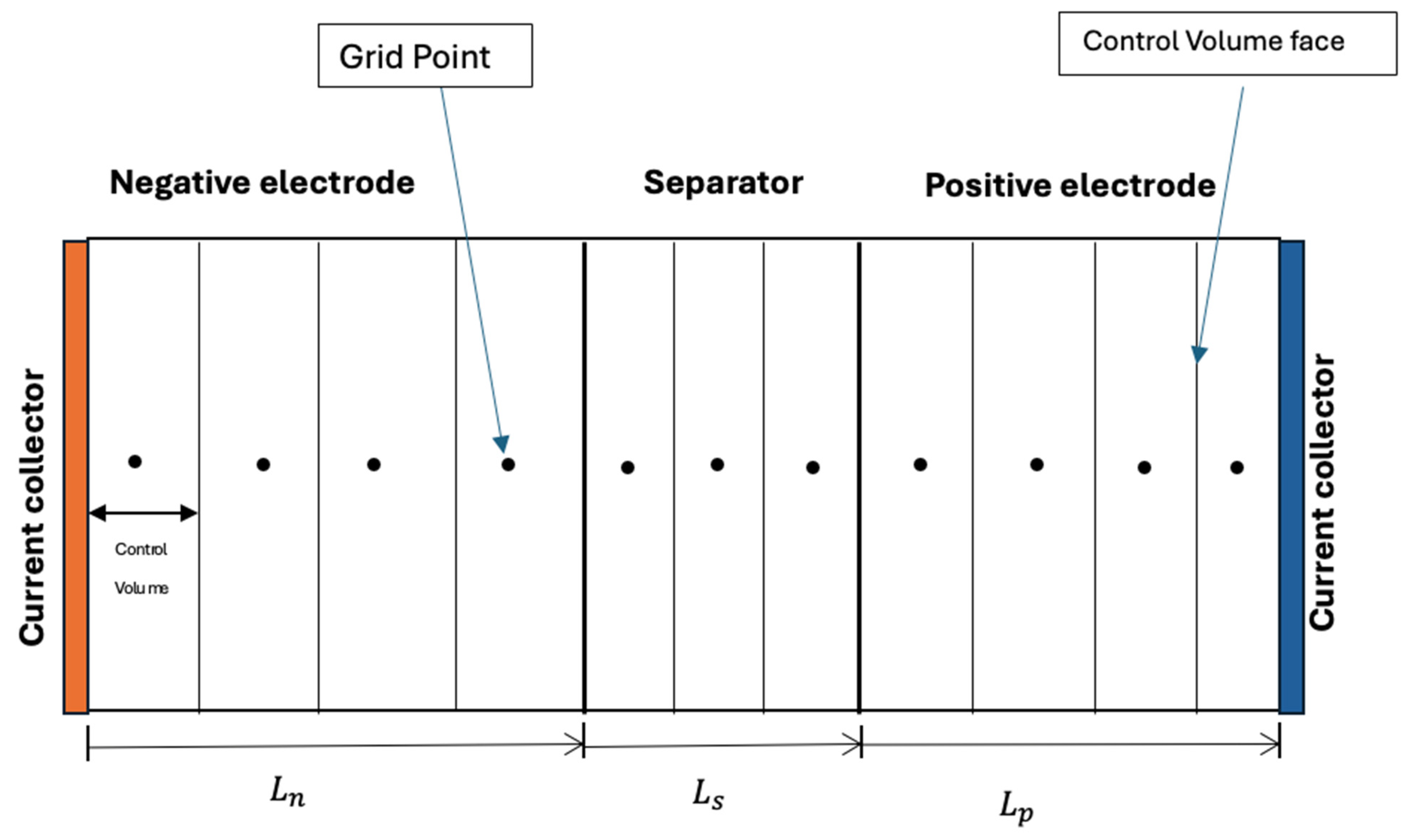
2.3. Computer Algorithm

The flowchart in Figure 2 presents the sequential steps that the developed MATLAB computer program utilizes to solve the set of PDEs that describe the electrochemical–thermal behavior of a lithium-ion battery. There are many operations that must be performed to implement the mathematical model presented in Table 1.

First, the cell parameters, as laid out in

Table 2. Program inputs from Gu and Wang [20].

Parameter	Unit	Negative Electrode	Separator	Positive Electrode
Geometry
Thickness	μm	128	76	190
Plate area	${\mathbf{c}\mathbf{m}}^2$	24		24
Router	μm	12.5		8.5
Material Properties
ρ	g/cm3	2.5	1.2	1.5
Kth	W/cm·K	0.05	0.01	0.05
CP	J/g·K	0.7	0.7	0.7
σ	S/cm	1	0	0.038
Diffusion Properties
Ds	${\mathbf{c}\mathbf{m}}^2/\mathbf{s}$	$3.9\times {10}^{-10}$		$1.0\times {10}^{-9}$
De	${\mathbf{c}\mathbf{m}}^2/\mathbf{s}$	$7.5\times {10}^{-7}$
Concentrations
Csmax	mol/cm3	0.02639		0.02286
${\mathit{C}}_{\mathit{e}}^{\mathit{o}}$	mol/cm3	$2\times {10}^{-3}$
Volume fractions
εe		0.357	0.724	0.444
εp		0.146	0.276	0.186
εf		0.026	0	0.073
εs		0.471		0.297
Activation energy
${\mathit{E}}_{\mathit{a}\mathit{c}\mathit{t},{\mathit{i}}_{\mathit{o}}}$	kJ/mol	30		30
${\mathit{E}}_{\mathit{a}\mathit{c}\mathit{t},{\mathit{D}}_{\mathit{s}}}$	kJ/mol	4		20
${\mathit{E}}_{\mathit{a}\mathit{c}\mathit{t},{\mathit{D}}_{\mathit{e}}}$	kJ/mol		10
${\mathit{E}}_{\mathit{a}\mathit{c}\mathit{t},\mathit{k}}$	kJ/mol		20
Constants
F	C/mol	96,485
R	J/Kmol	8.314
Others
αa, αc		0.5		0.5
i0	$\mathbf{A}/{\mathbf{c}\mathbf{m}}^2$	$0.11\times {10}^{-3}$		$0.08\times {10}^{-3}$
${\mathit{t}}_{+}^0$		0.363
p		1.5
h	$\mathbf{W}/{\mathbf{c}\mathbf{m}}^2\mathbf{K}$	0 (adiabatic), 1 or 2
${\mathit{T}}_{\mathit{\infty }}$	K	25

, are input into the program. These parameters are obtained from Gu and Wang [4] for a negative electrode made up of Li_xC₆, a positive electrode made up of Li_yMn₂O₄ and a porous polymer separator. The electrolyte is a solution of lithium salt in a non-aqueous solvent. Some input variables are the starting conditions such as the initial SOC, number of control volumes, convective heat transfer coefficient, etc. The input variables specify the starting conditions and the operating conditions of the battery. After all the required inputs are read into the MATLAB program, an initialization process is carried out. For the most part, initialization is performed on array quantities and quantities that require simple calculations. So that the developed program can vary the current as a function of time, a time current subroutine has been written. This subroutine sets the current or current variations for charge or discharge conditions as a function of time. The last operation that is completed before entering the time loop is to set up the discretization geometry. This is carried out in the geometry subroutine which determines such things as grid spacing, control volume sizes, control volume face locations and many more geometric quantities associated with the discretized grid.

There are two major loops in the program: one is the time loop and the other is a while loop. The time loop steps through the operation time of the battery. The amount of time simulated can be set by the operator. Essentially, every time step requires a separate simulation for the battery cell behavior. Just inside the time loop is the while loop. The while loop performs the iterations required to converge all of the equations being solved. The electrochemistry–thermal model presented in Table 1 results in a set of nonlinear, coupled differential equations. This can only be solved by mimicking the nonlinear equations with linear equations that use guesses on the quantities that make the equations nonlinear. Thus, an iterative solution is required. The quantities that require a tri-diagonal matrix algorithm (TDMA) solver are identified in Figure 2.

As shown in the flow chart, several quantities need to be calculated for each iteration of the while loop. The equations for these quantities are continually solved using updated guesses for their values until all equations reach a point where the guessed values for all the dependent variables no longer change. Convergence is taken to better than or equal to 10⁻⁴ of a fractional change or in the case of some parameters, an absolute change within the units of the quantity being converged.

After the convergence of the while loop quantities, the program drops out of the while loop and moves to the next time step. The same procedure for the new time step is performed until all time steps have been calculated. After completing computations for the input time period, the program produces some battery performance quantities and a number of interesting plots.

3. Results

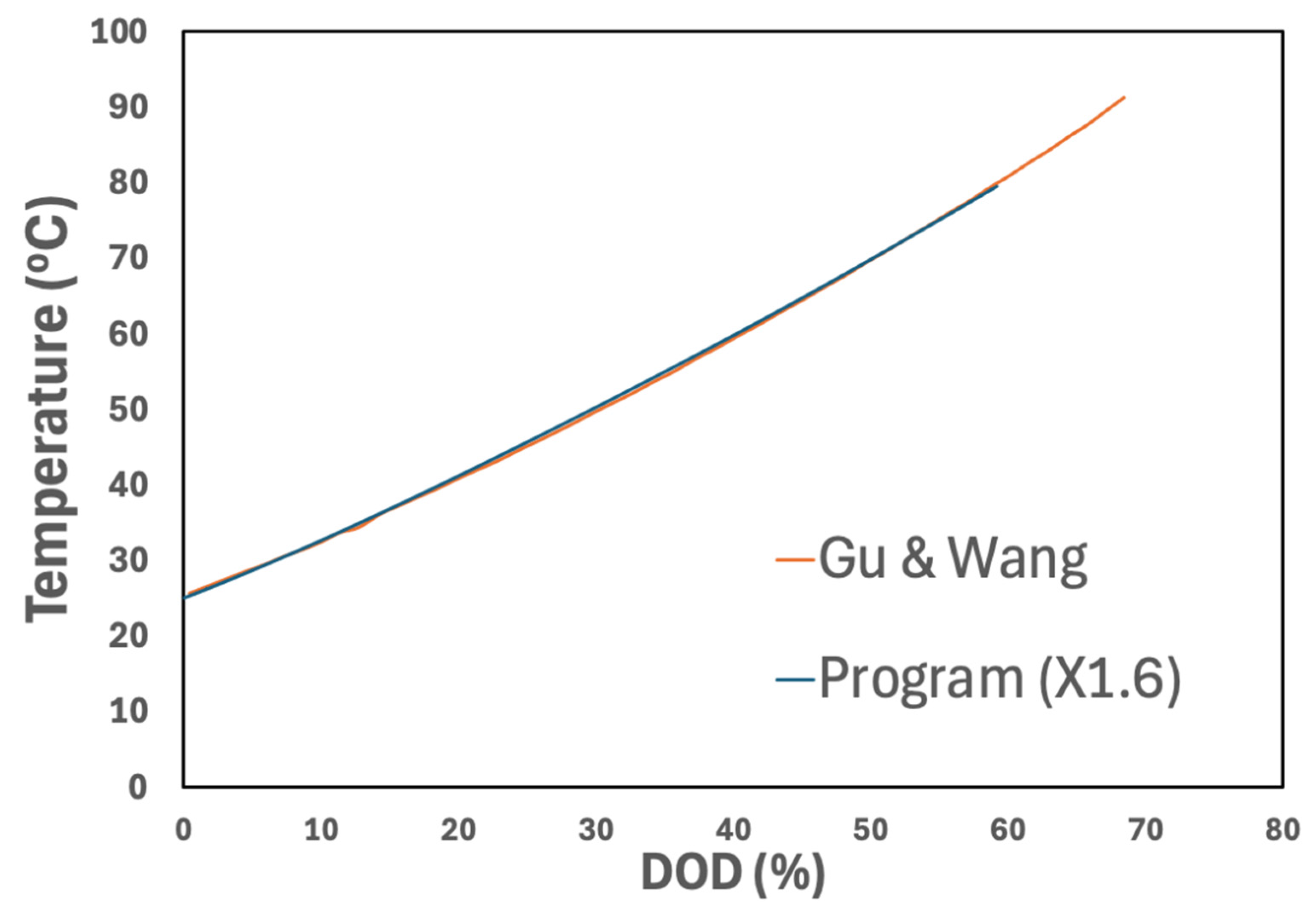
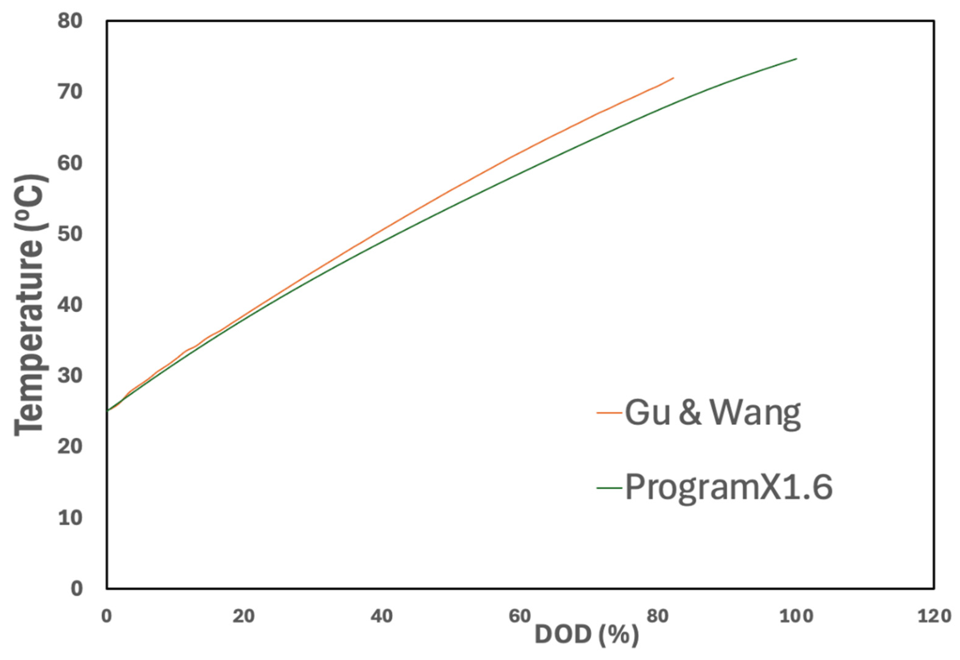
3.1. Electrochemical Model Verification

Two comparisons are presented in this section. First, the comparisons for a static current load for discharging, charging and the equilibrium and second, comparisons for a dynamic current load that cycles between discharging, rest and charging. The second case mimics that required for a HEV (hybrid electric vehicle) and can be referred to as a pulsed operation. For both comparisons, the required input quantities come from Table 2 of Smith and Wang’s [13] paper, except the positive electrode thickness. The reader should note that this table is not repeated in this paper. For the results presented in Section 3.2 and Section 3.3 of this paper, the input quantities of Gu and Wang [20] are used, which are presented in Table 2 of this paper. Smith and Wang’s battery cell is much bigger than that of Gu and Wang. The electrode area of Smith and Wang’s battery cell is 1.0452 m², while that of Gu and Wang is 0.0024 m². The application of Smith and Wang’s battery cells is in HEVs, while that for Gu and Wang, it appears to be electronic devices.

Smith and Wang [13] give a positive electrode thickness of 3.64 × 10⁻⁵ m in their paper. In this work, a positive electrode thickness of 4.354 × 10⁻⁵ m is used. Many attempts were made to match Smith and Wang’s results using their published positive electrode thickness, but the results always showed a battery cell lacking capacity. Finally, a hand calculation was made for the capacity of each electrode using the equations

$${ Q}_{-}{=\epsilon }_{sn}{L}_{n}A{C}_{smax-}\left(∆xx\right)F$$

(5)

and

$$Q_{+}={\epsilon }_{sp}{L}_{p}A{C}_{smax+}\left(∆yy\right)F.$$

(6)

Equation (5) provides the charge-carrying capacity of the negative electrode, ${ Q}_{-}$, and Equation (6) provides the charge-carrying capacity of the positive electrode, $Q_{+}$. These two quantities are expressed in coulombs, or equivalently amp-hours if you divide by 3600 s/h, and represent an upper limit on the amount of charge (the length of time a given current flow can be maintained) that can be delivered by the battery. The quantities $∆xx$ and $∆yy$ are the rated maximum fractional changes that can occur in the concentrations of the lithium particles, as given by

$$∆xx={xx}_{100\%}-{xx}_{0\%}$$

(7)

and

$$∆yy={yy}_{0\%}-{yy}_{100\%},$$

(8)

where the subscript of 100% is the fractional concentration of lithium particles in the active particles at 100% SOC and the subscript of 0% is the fractional concentration at a 0% SOC. The symbol $xx$ is for the negative electrode and the symbol $yy$ is for the positive electrode. The negative electrode gives up lithium particles and thus decreases in concentration and the positive electrode absorbs lithium particles and thus is increasing in concentration as the battery is discharging.

Applying Equations (5) and (6) to the electrode thicknesses reported by Smith and Wang [13] results in a negative electrode charge-carrying capacity of 7.19 A·h and positive electrode charge-carrying capacity of 6.02 A·h. The capacity of the battery being simulated was reported by Smith and Wang to be 7.2 A·h. Thus, the positive electrode has too low of a charge-carrying capacity and limits the overall capacity of the battery to 6.02 A·h. This is the reason why the simulations performed earlier in this work were running out of charge before those presented by Smith and Wang. This is also the reason why Borakhadikar [11] was not obtaining good comparisons to the results of Smith et al. [12] which used the same thickness as Smith and Wang [13]. Borakhadikar changed the thickness of both electrodes and the separator based on values he found in other papers, thus obtaining reasonable comparisons. Based on calculations using Equations (7) and (8), it looks like only the thickness of the positive electrode should be changed from a value of 3.64 × 10⁻⁵ m to 4.35 × 10⁻⁵ m. This is what is carried out for the results presented in this section.

Figure 3 shows the comparison of the static current load results from this work to those from Smith and Wang [13] while discharging the battery at 1 C, for charging the battery at 1 C and for equilibrium conditions (OCV) as a function of the capacity of charge left in the battery. This is the way Smith and Wang present their results and the same is carried out here. The solid lines in Figure 3 are from the work of Smith and Wang and the dashed lines of the same color are from this work using the increased positive electrode thickness of 4.35 × 10⁻⁵ m. It is observed that good comparisons are obtained in all three cases: discharging, charging and equilibrium. The equilibrium results are solely based on the equilibrium potentials. The lower set of curves, the battery discharging at a constant rate, shows very good comparisons, except for some small deviations at low battery capacities, which are less than 1 A·h. These deviations are small, but noticeable. It is in this region that calculations become more difficult to converge and are more dependent on input conditions matching. The top set of curves are for charging the battery. The results from this work are slightly above those of Smith and Wang. More than likely, this is due to small differences in the region where the battery capacity is less than 1 A·h. This region shows small deviations in the discharge curve and it is believed that this carries over to the charging curve. Since the charging calculations are performed from 0% capacity to 100% capacity, the errors incurred in the lower capacity are carried through all capacities. The discharge curve is computed from the full-capacity side of the plot to the low-capacity side and thus the errors at the lower capacities do not show up until the end of the simulation.

The next comparisons made between the results of Smith and Wang [13] and those from this work are for the pulsed operation of a lithium-ion cell. The same input values, as used for the static current comparisons shown in Figure 3, are used here. The difference is that the current loads applied to the battery cell are dynamic and change quickly as a function of time. The current load profile is shown in Figure 4. This current curve can be referred to as a Hybrid Pulse Power Characterization (HPPC) curve. The HPPC current curve shown in Figure 4 is one of the current loads used to determine the dynamic power capability of batteries for the FreedomCar project (see Sun and Kainz [22]). The HPPC test curves shown in Figure 4 consist of short-duration discharge and charging pulses separated by relaxation periods and start with some short, fraction-of-a-second pulses. This HPPC procedure shown in Figure 4 starts with a 0.1 s, 55 A current discharge–charge pulse; a constant 30 A, 18 s discharge; followed by an open-circuit relaxation (no current) for 32 s; then a 0.1 s, 55 A current discharge–charge pulse; followed by a 22.5 A charge for 10 s; and finally, open-circuit relaxation. This operation lasts for 65 s and helps to evaluate the dynamic power capabilities of a lithium-ion cell by looking at the voltage response of the battery to the pulsed current loads. The high-rate 0.1 s pulses were for testing the battery’s high-frequency resistance.

The voltage responses to the input current loads shown in Figure 4 are given in Figure 5. These results are obtained and plotted for various initial SOC conditions: 30%, 40%, 50%, 60% and 70% of the initial SOC nominal values. The actual SOCs used were 41.7%, 50%, 58.3%, 66.6% and 75%, respectively. The nominal values are for the nominal cell capacity of 6 A·h and the actual values used in the calculations correspond to the actual cell capacity of 7.2 A·h. To calculate these results, a film resistance, $R_f$, of 20 ohm-cm² was inserted into the cell potential equation shown in Table 1. This film resistance was used to account for the effects of both the SEI layer resistance and film resistance.

Just like Figure 3, Figure 5 shows the results from Smith and Wang [13] as solid lines and the results from this work as dashed lines of the same color. As would be expected, the initial voltage is highest for the highest initial SOC of 70% and lowest for the lowest initial SOC of 30%. The voltage dip observed in Figure 5 just after the first second, which is followed by a subsequent voltage rise, corresponds to the initial high-rate pulse in Figure 4. This is followed by 18 s of steady voltage decay, as observed in Figure 5, due to the uniform 30 A current draw, as shown in Figure 4. Open-circuit relaxation results in a slightly rising voltage behavior for all initial SOCs because of the battery coming to an equilibrium condition at its current SOC. A 0.1 s, high-rate pulse then follows, which results in a sudden voltage dip and rise. The negative uniform current observed in Figure 4 indicates battery charging which corresponds to the steady voltage rise observed in Figure 5. Finally, open-circuit relaxation follows which causes the battery to settle towards the equilibrium, hence the voltage drops to a steady value for the different SOC plots.

Comparisons to the results of Smith and Wang [13], shown in Figure 5, are good but show some deviations during the discharge and charging phases. The voltage comparisons for the open-circuit relaxation regions show better agreement between the two sets of results than the discharging and charging phases of the current profile. It is further observed that an initial SOC of 70% shows the least deviation between the cell voltages predicted by this work and the voltage behavior calculated by Smith and Wang for the discharging phase of the current profile. For the charging phase of the current profile, the 30% and 40% initial SOC cases have the best comparisons. It is not understood why there are better comparisons of the results in certain regions and poorer comparisons of the results in other regions; however, deviations in results can carry over from one time to a later time. That is to say, the cell voltage is a function of the history of the cell not just the present time.

The magnitude of the differences between results from this work and those from Smith and Wang [13] is generally less than 20 millivolts and more often in the order of just a few millivolts. For peak-to-trough voltage changes of about 3.9 volts to 3.3 volts, this would mean that the maximum deviation between the sets of results is about 3%. This is considered good. Better comparisons are obtained for the static current cases than the dynamic current cases.

Rapidly changing current conditions put more stress on a battery model than a slow charging and discharging process where the load current does not change. Borakhadikar [11] had good comparisons to Smith et al. [12] for static discharge–charging conditions, but to obtain these good comparisons, the size of the electrodes had to be changed from what was specified in Smith et al. [12]. In this work, it was discovered that the size of the negative electrode as reported by Smith et al. [12] and Smith and Wang [13] cannot be correct and what Borakhadikar carried out was justified. However, only one electrode thickness needed to be changed, as opposed to changing both thicknesses as Borakhadikar [11] did. Additionally, the separator thickness did not need to be changed.

3.2. Electrochemical–Thermal Model Results

In this section, the results that include the effects of temperature are presented. Temperatures within the battery cell are obtained with the thermal model presented in Table 1. In this section, two types of results are discussed: decoupled and coupled. The decoupled results take the cell material properties to be independent of temperature. This means the electrochemical cell behavior is only dependent on temperature through the transfer current given by the Butler–Volmer equation. On the other hand, the coupled model considers the temperature dependence of material properties like diffusion, conductivity and the exchange current density, as well as through the transfer current. Of course, the coupled model provides more physically realistic results, but the decoupled model allows the reader to gage the material property temperature effects on different results. All the results in this section use the 0.0024 m² surface area cell from Gu and Wang [20], whose input quantities are given in Table 2.

3.2.1. Cell Voltages

Figure 6 shows the cell voltage variation as a function of DOD for a 3 C operating condition using adiabatic boundary conditions ($h$ = 0 W/m²-K). Three curves are shown on this graph. The highest curve is the coupled simulation results and the lowest curve is the decoupled simulation result from this work. Curves generated with the MATLAB computer program developed in this work are labeled Program in the plots. In between these two curves lie the results from the coupled analysis of Gu and Wang [20]. The results of Gu and Wang lie close to the coupled results of this work. Other than the differences in the location where the battery cell is no longer able to deliver 3 C current, the comparisons are reasonable. Gu and Wang’s results show a battery that is unable to deliver 3 C of current at 80% DOD, while the coupled results from this work make it out past 100% DOD. The uncoupled results of this work indicate that the battery is unable to meet the 3 C current demand at a 60% DOD. These differences may be because of the way Gu and Wang perform their thermal modeling and the way that this work performs its thermal modeling. More will be said about this in the next subsection. Also demonstrated by the graph in Figure 6 are the differences between coupled and uncoupled simulations. The coupled results provide higher cell voltages at higher DOD values. This occurs because of the way temperature affects the magnitude of the material properties of the battery. This is a significant effect in both the cell voltage magnitude and the total amount of charge delivered by the battery. These results point to the need to incorporate the temperature dependence of battery material properties since this significantly affects the accuracy of results.

3.2.2. Cell Temperatures

The results in Figure 7 demonstrate a comparison of this work’s temperature results with the temperature results of Gu and Wang [20] for a 3 C current load in the discharge mode for adiabatic boundary conditions ($h$= 0 W/m²-K). The temperatures shown in this plot are averaged over all locations in the cell at a given time or a given DOD. Both coupled and uncoupled curves from this work and from Gu and Wang are on this graph. It is interesting that the uncoupled simulations show higher temperature values than the coupled simulation results. These differences increase as the cell discharges. Essentially, heat builds up in the cell as the battery continues to provide current to the load. This means that results are dependent upon the history of the battery operation. For the results here, the battery starts fully charged and runs until it is fully discharged. Another interesting observation is that the uncoupled results are concave upwards while the coupled results are concave downwards. Thus, the rate of the temperature increase is slowing for the coupled simulations and increasing for the uncoupled simulations.

While the temperature behavior with DOD, as shown in Figure 7 from this work, has similar trends and shapes as the results from Gu and Wang [20], the magnitudes are not well correlated. This holds true for both the uncoupled results and the coupled results. This is likely because of the difference in the thermal modeling approaches used in this work and those used in Gu and Wang. Gu and Wang used a lumped heat source model in their analysis, where the source term in the energy equation is taken to be the same value across the entire cell. This is a crude approximation in that the source term is a function of the transfer current which can change significantly from one location in the cell to another. In this work the source term is calculated at every control volume based on the cell quantities present at that location. This can easily be completed because the MATLAB computer program developed here uses a finite volume discretization technique such that the battery geometry is divided into small control volumes where each control volume can have different source terms based on different conditions. The lumped model used by Gu and Wang is computationally less costly than the discretized approach used in this work, but the varying heat generation source used here is understood to be a more accurate representation of the electrochemical–thermal behavior of the cell.

Details on how Gu and Wang [20] determined a lumped source term for the battery cell are not given; however, Gu and Wang do provide some thermal source term results as a function of DOD. If the thermal source terms calculated in this work are volume averaged over the entire cell, it appears that this work’s average source term needs to be multiplied by approximately 1.6 to equal those of Gu and Wang. When this is carried out for the uncoupled simulations, the results shown in Figure 8 are obtained. The results from this work compare excellently to those of Gu and Wang. When this same volume of the averaged source term multiplied by 1.6 is used to compare to the coupled temperature profiles shown in Figure 9, good comparisons are still seen, but not as good as for the uncoupled results in Figure 8. It is easy to understand the differences in the temperature results from this work and those of Gu and Wang shown in Figure 7. Since our model is more detailed than that of Gu and Wang and considers these values to vary spatially within the battery, the lumped model presented in Gu and Wang understandably returns a different temperature profile owing to the different handling of the heat generation terms.

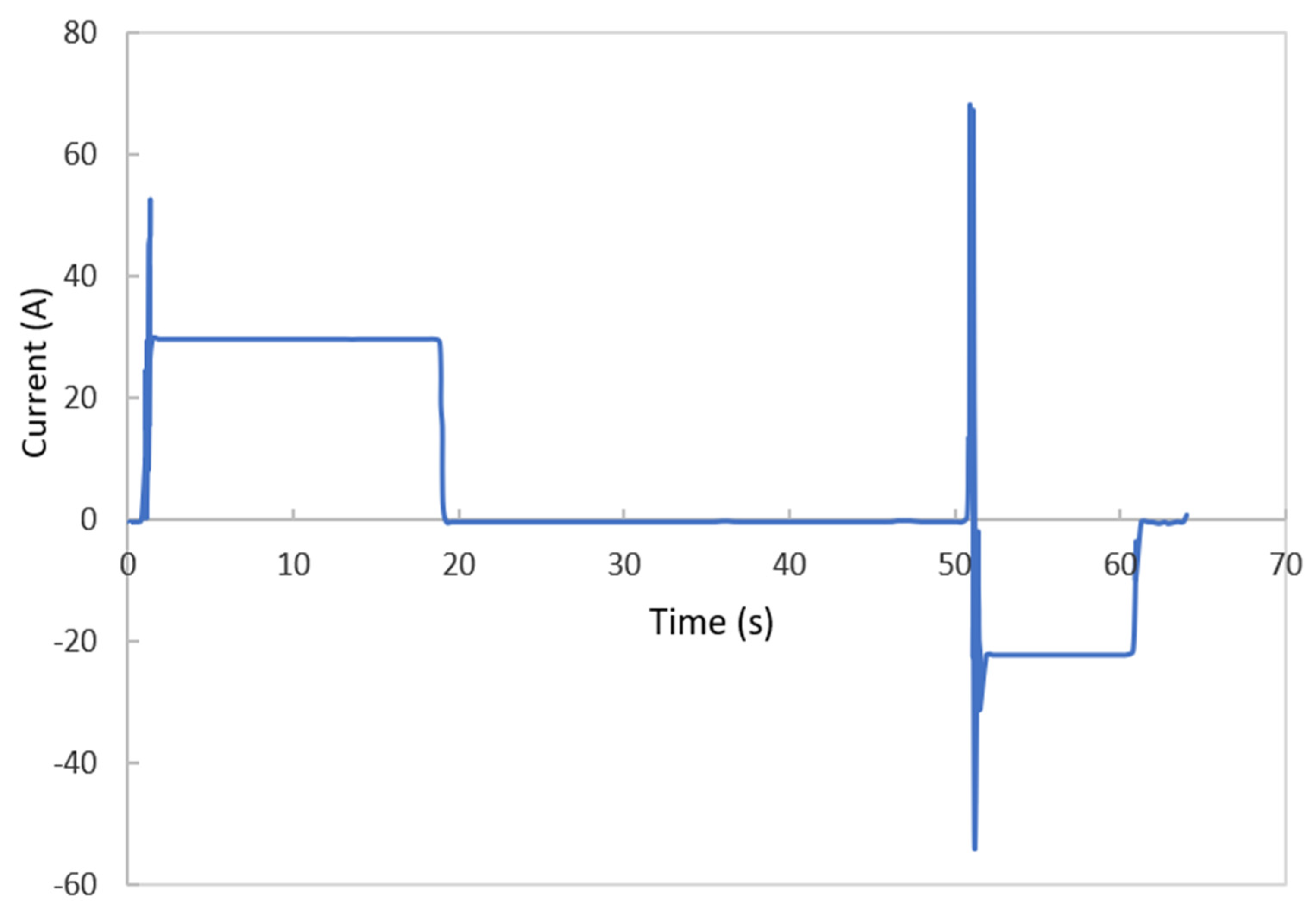
3.2.3. Effect of Current Load

Current flowing through the internal resistance of a battery results in joule heating, as well as other types of thermal loads. Higher currents result in higher joule heating values which cause higher temperatures. Figure 10 shows that cell temperatures increase faster with increased current loads. At current loadings of 10 C, the temperatures increase extremely fast. This indicates that care should be taken when running batteries at high current loadings.

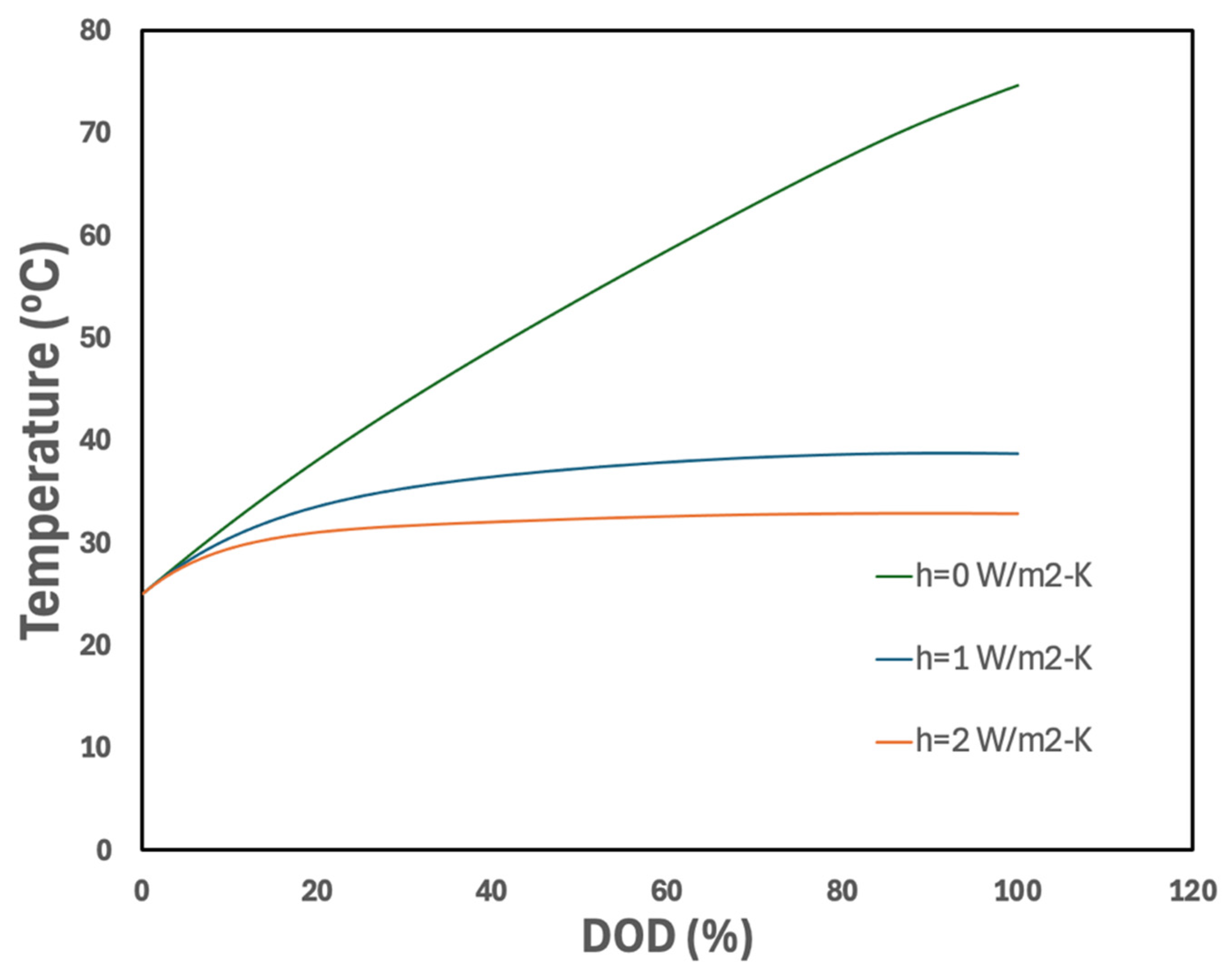
3.2.4. Effect of Boundary Heat Transfer Coefficient

The temperature results discussed thus far assumed adiabatic boundaries for which the convective heat transfer coefficient is zero. Other heat transfer coefficient values that produce higher cooling rates are compared to the adiabatic case for a 3 C discharge rate, as shown in Figure 11. The variation of temperature for a constant discharge rate of 3 C is illustrated for convective heat transfer coefficients of 0, 1 and 2 W/m²-K. It is shown that higher values of a convective heat transfer coefficient result in a lower rate of increase in the battery internal temperature. Such results are critical for thermal runaway studies and the design of battery thermal management systems.

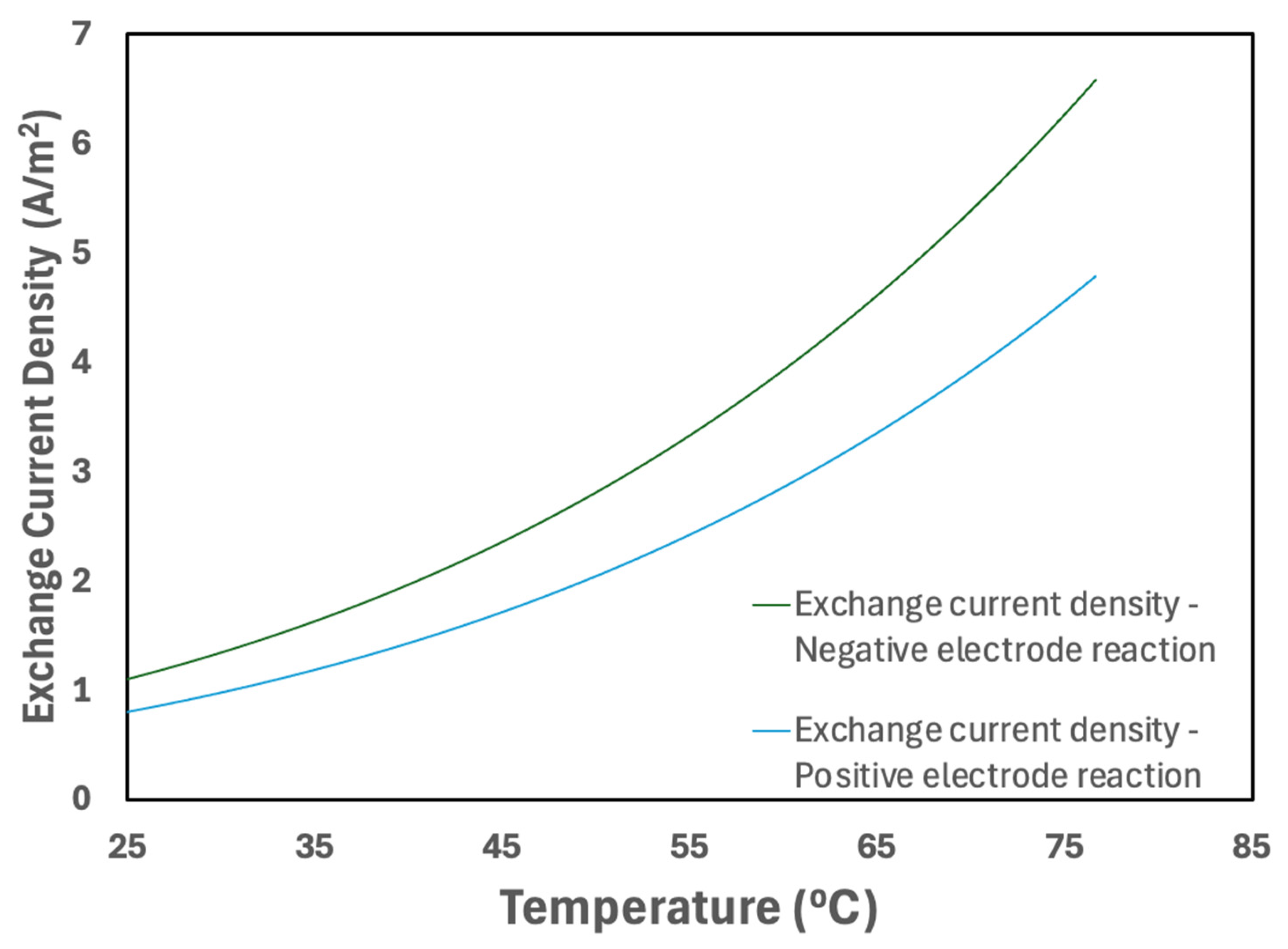
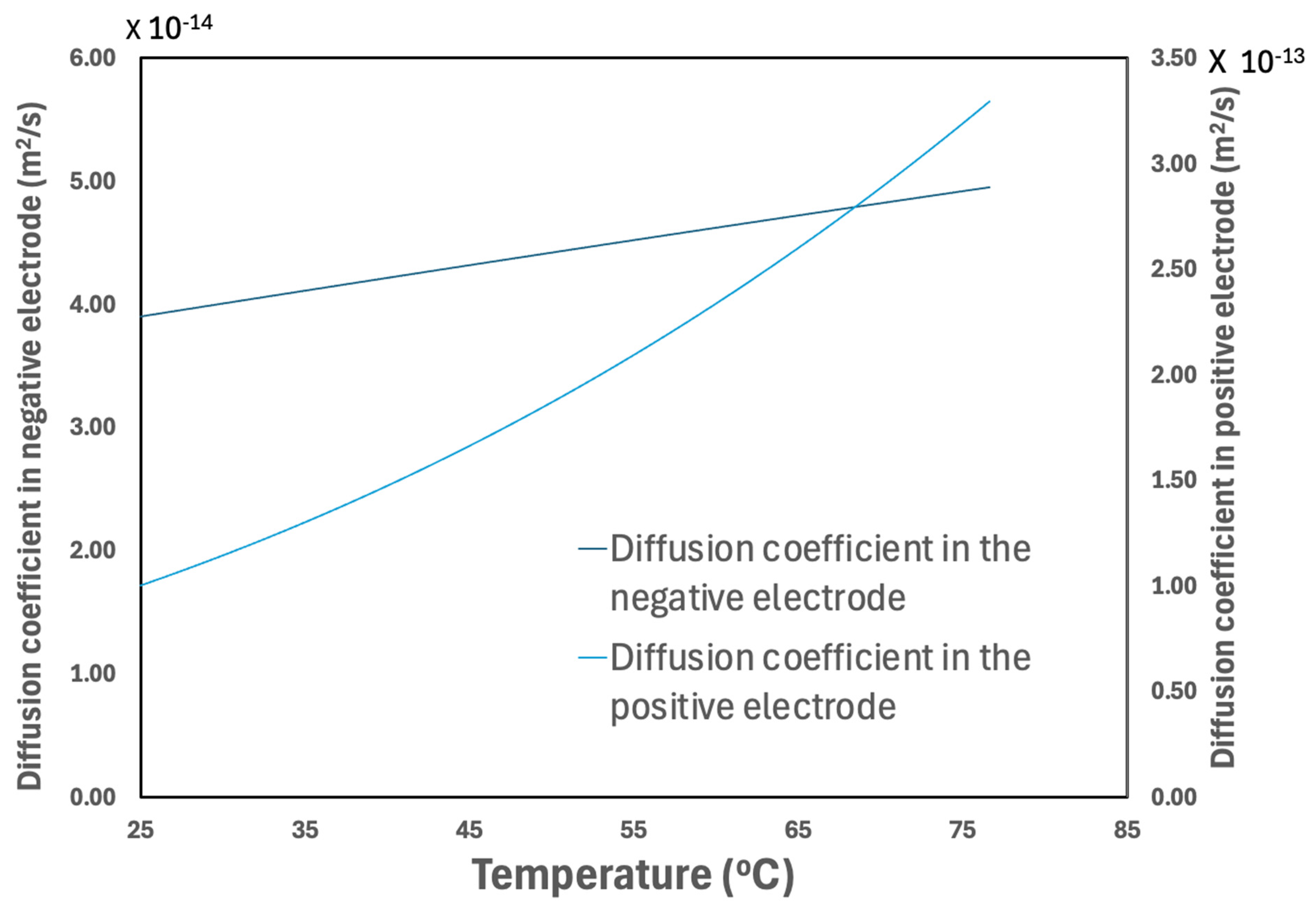
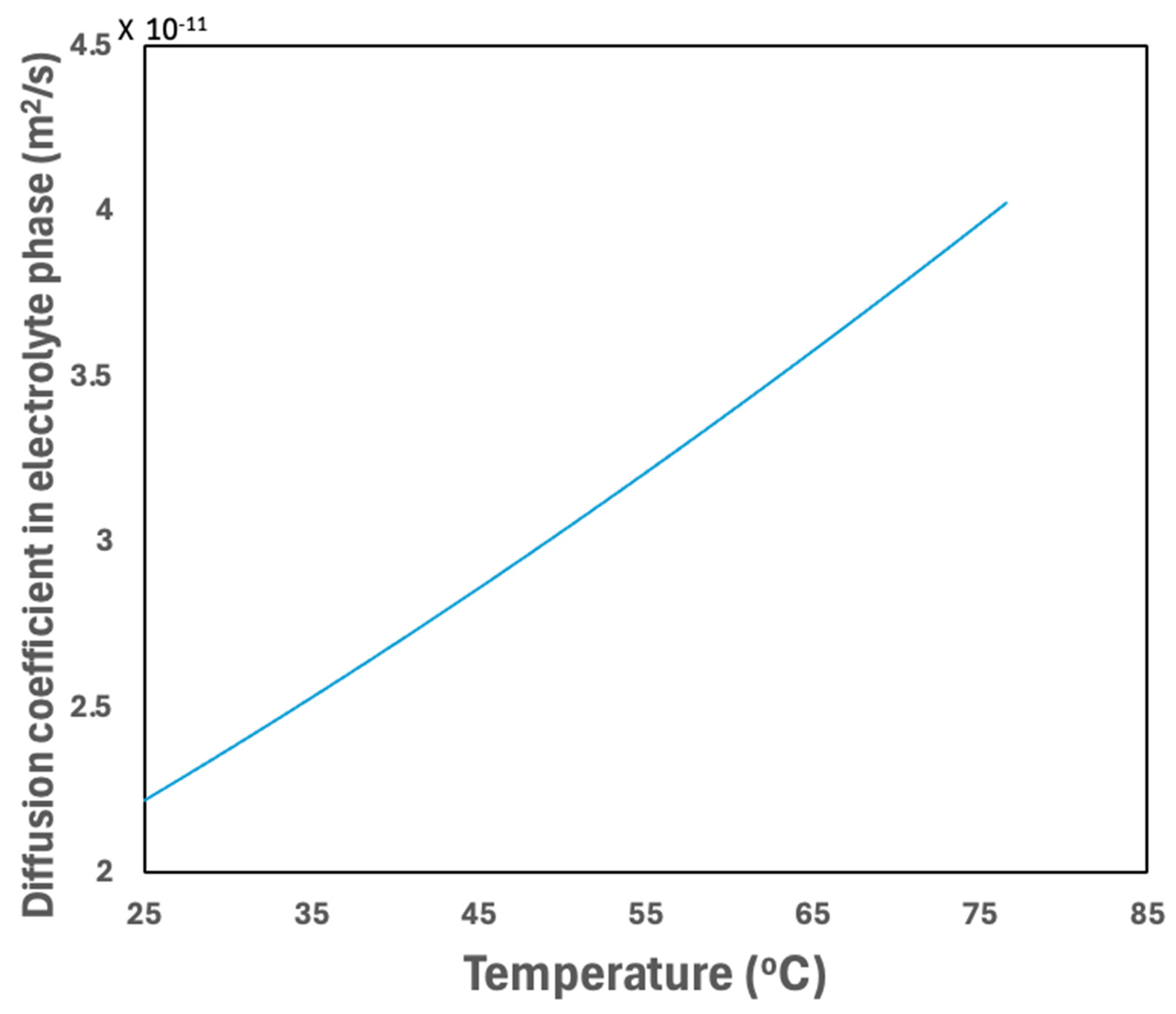
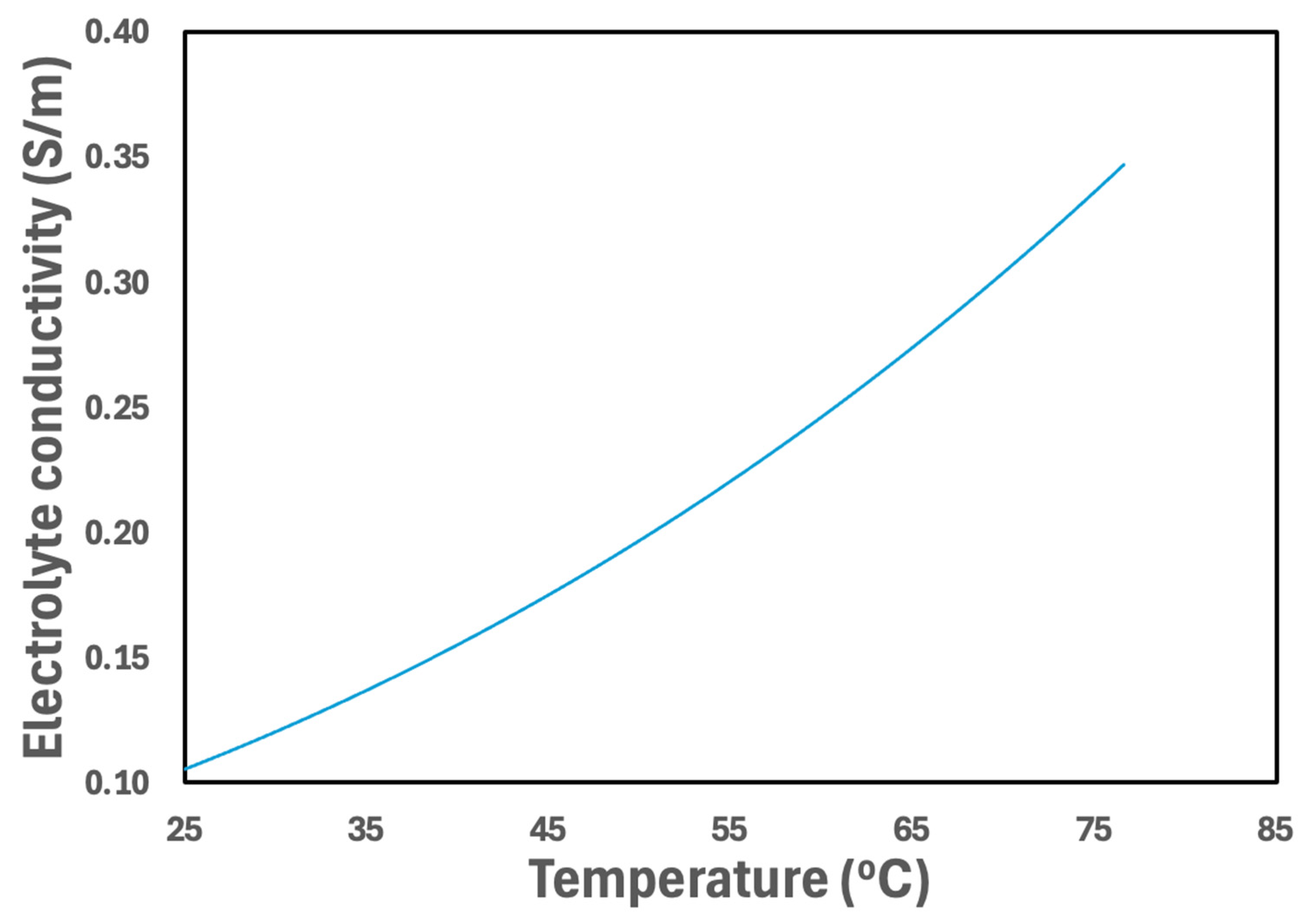
3.2.5. Temperature Effect on Material Properties

Since there is a significant difference in the coupled and uncoupled results shown above, it is beneficial to consider the change of material properties with the temperature. The specific parameters for which temperature dependence has been considered below are the exchange current density, diffusion coefficients in solid and electrolyte phases, as well as ionic conductivity. The adjustment of these values through the Arrhenius’ equation for property changes with temperature (see Table 1) yields the temperature dependencies shown in Figure 12, Figure 13, Figure 14 and Figure 15. Temperature ranges run from 25 °C to 75 °C. The stated material property values shown in Table 2 are at a reference temperature of 25 °C. This is a reasonable temperature range given the temperature plots shown in prior subsections. Over this temperature range, the presented properties change by a factor of two to six.

Given the property value changes shown in Figure 12, Figure 13, Figure 14 and Figure 15, it is reasonable that we see significant differences in the coupled and decoupled results shown in Figure 6 and Figure 7. The coupled results seem to produce higher cell voltages and lower temperatures. Higher cell voltages and lower temperatures can result from an increase in the material properties presented in Figure 12, Figure 13, Figure 14 and Figure 15. Increasing diffusion coefficients and increasing electrical conductivities should reduce irreversible losses in the battery, increasing the cell voltage and decreasing the cell temperatures obtained with the coupled simulation compared to the uncoupled simulation. The uncoupled simulation uses property values at 25 °C, while the coupled simulation uses the 25 °C properties at the start, but quickly replaces the 25 °C properties with higher temperature properties which are significantly larger.

3.3. Spatial Results

The purpose of the results presented in this section is to let the reader know how different dependent variables vary across the electrodes and separator, that is, how they vary with the location in the battery cell or how they vary with the radial position in the spherical particles. This includes the temperature, lithium particle concentrations at the surface of the active particles, lithium particle concentrations in the active particles, lithium particle concentrations in the electrolyte and overpotentials. All of these quantities are evaluated for a battery cell discharging current of 3 C. The boundary conditions at the side of the cell are adiabatic, that is, $h$ = 0 W/m²-K. Spatial curves are shown at a number of DODs where the computation starts from the fully charged condition. Since the condition of the battery at any DOD is a function of where it starts, different results would be obtained if the current discharge were started at a DOD different than 0%. All the results shown start at a DOD of 0%.

3.3.1. Temperature

Figure 16 shows the temperature profiles throughout the cell. The interesting aspect of these results is the temperature which is essentially the same value at all locations in the cell at a given time. Essentially, time is represented by a DOD in this plot. The temperatures increase with time because the net energy is being converted from chemical energy to thermal energy and the thermal energy has nowhere to go, it can only build up in the cell. Even if thermal energy were allowed to escape from the sides of the cell by setting the convective heat transfer coefficient to a small, nonzero value, the temperature profiles would still be flat. The reason for this is the small thicknesses of the electrodes and the separator, that is an overall cell thickness of 394 μm. This small thickness makes the thermal resistance to heat flow inside the cell much less than the thermal resistance to heat flow from the sides of the cell to the surroundings by convection.

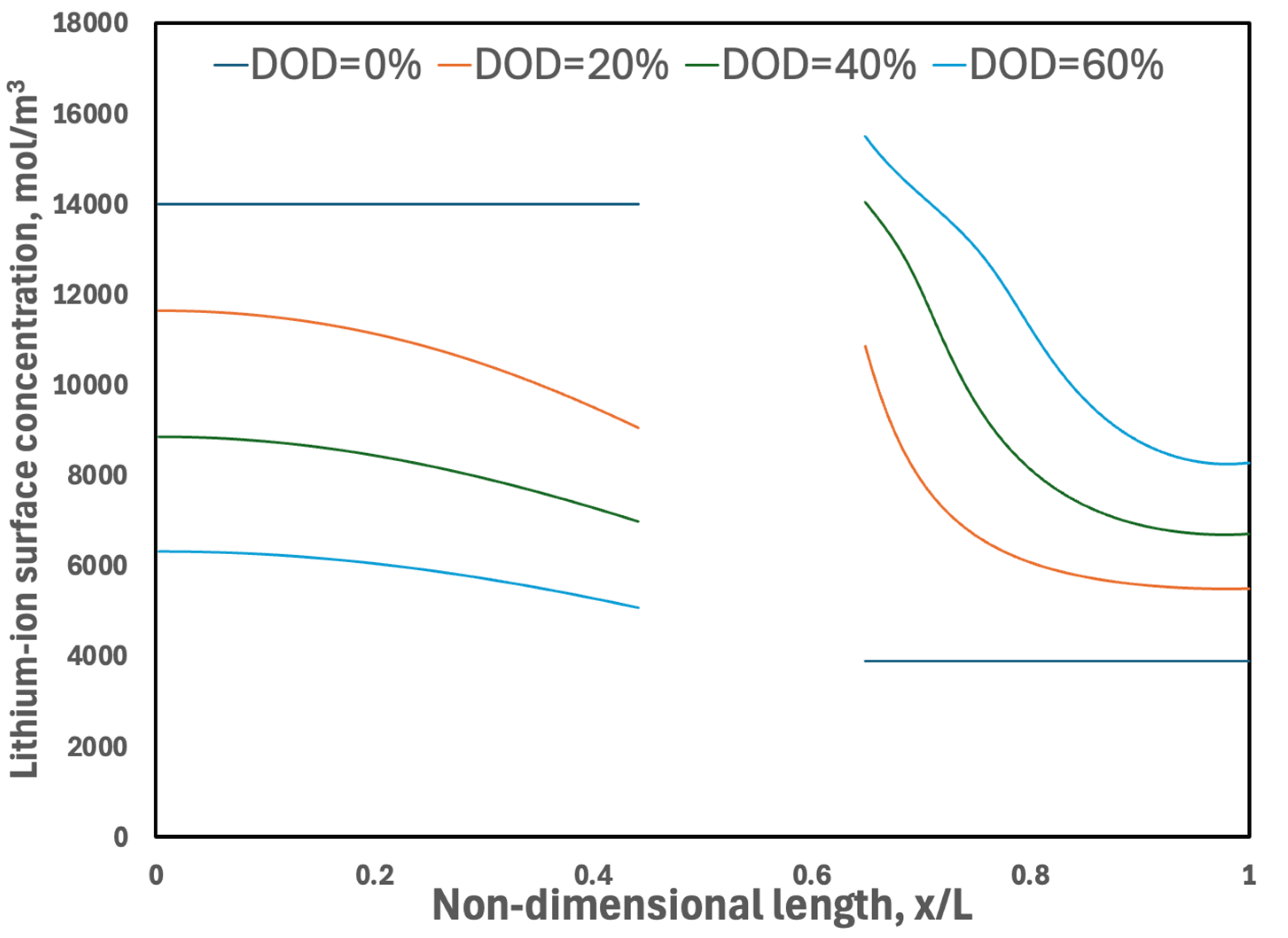
3.3.2. Surface Concentration

The lithium particle concentrations at the surface of the spherical particles as a function of the x-location in the cell are given in Figure 17. This figure shows this for both the negative electrode and the positive electrode. Of course, there are no active particles in the separator and thus there are no surface concentration values here. It is first observed in this figure that the slopes of these lithium particle concentrations are negative, that is, they slope downwards from the left to the right. This has to be the case because lithium ions need to flow from the negative electrode on the left to the positive electrode on the right when the battery is discharging. When the battery is charging, these slopes will become positive. An interesting feature of the slopes is that the curves are steeper in the positive electrode than the negative electrode. More than likely, this is due to the lower active particle volume fractions and thicker electrode on the positive side of the battery. It is also noticed that the lithium-ion surface concentrations in the negative electrode decrease with the increasing depth of discharge. Similarly, the concentration of lithium ions at the surfaces of the spherical particles in the positive electrode increase during discharge due to the intercalation of lithium ions flowing from the negative electrode through the electrolyte. As observed in Figure 17, the surface concentration for increasing DOD values tends towards the maximum concentration stated in the program inputs in Table 2.

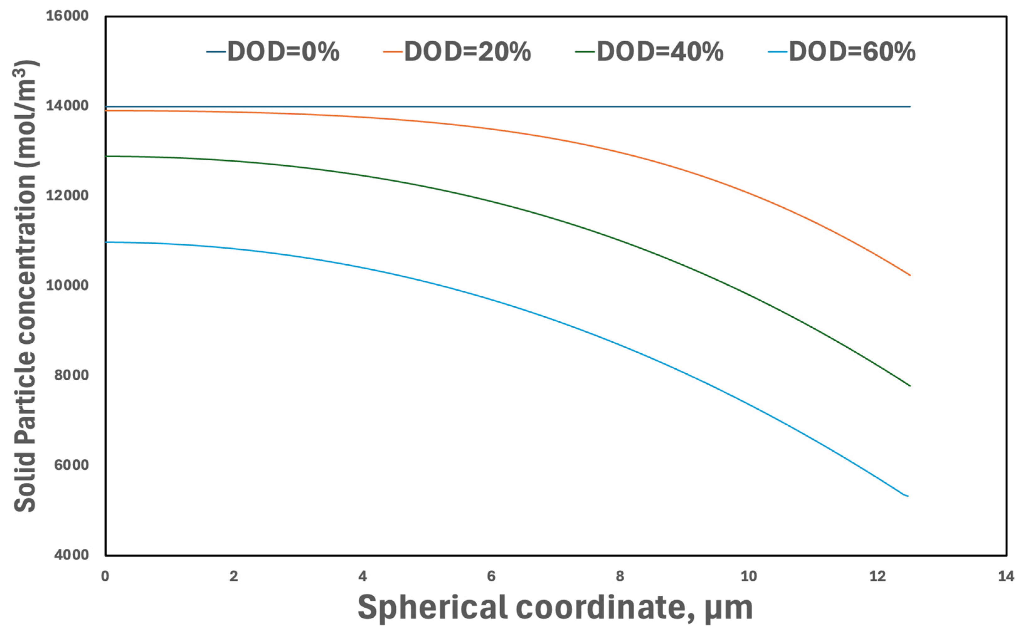
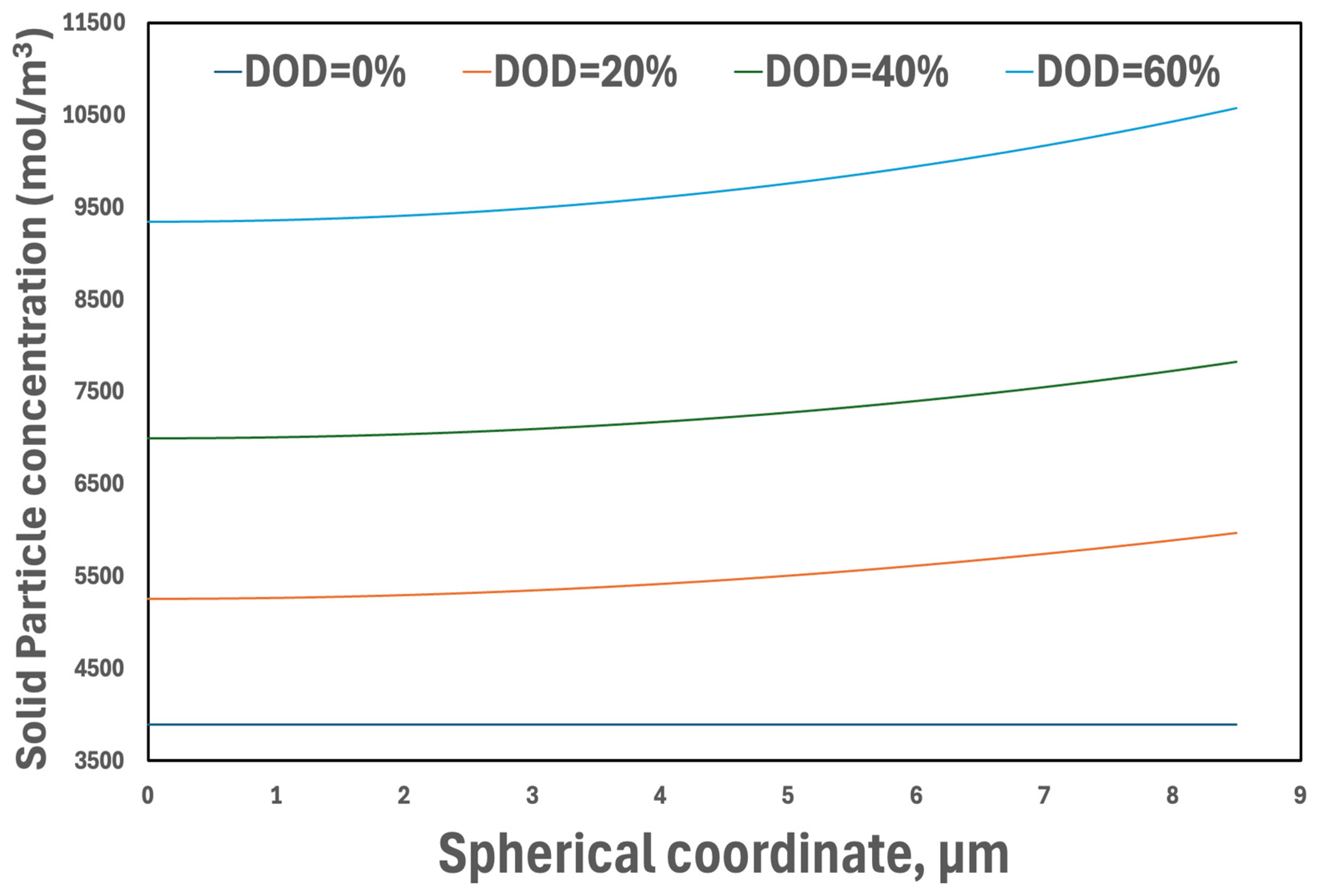
3.3.3. Concentrations in Active Particles

Just like the work of Doyle et al. [7], a pseudo two-dimensional model (P2D) is used in the simulation of this work, which assumes a geometry comprised of both a Cartesian coordinate system and spherical coordinate system. Figure 18 and Figure 19 illustrate the concentration of lithium ions in the spherical particles in the negative and positive electrodes, respectively, at one$x$-location for each electrode. The $x$-location is at the center of each of the electrodes.

Both Figure 18 and Figure 19 show a uniform distribution of lithium particle concentrations at the start of the discharge process. As expected, the lithium-ion concentration decreases with increasing values of DOD at the negative electrode due to the deintercalation of lithium ions during discharge. Similarly, Figure 19 shows an increasing lithium-ion concentration in the spherical particles during discharge, due to intercalation of lithium ions. The spherical-particle lithium concentrations are at a minimum at the center and increase to maximum values at the surface of the active particles for the positive electrode and the negative electrode has a maximum at the center with a decreasing trend towards the surface of the active particles. This allows lithium ions to flow out of the active particles in the negative electrode and into the active particles in the positive electrode.

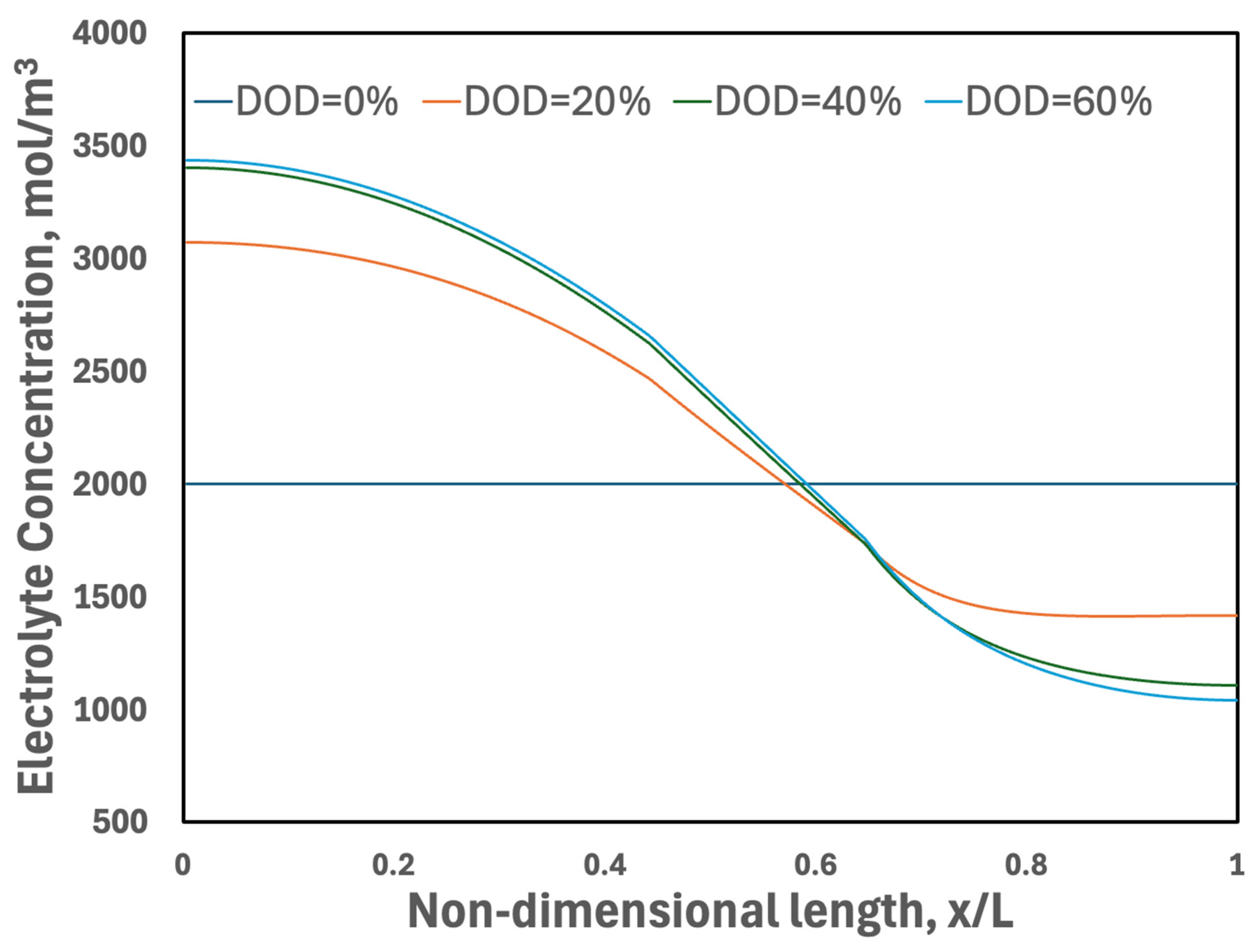
3.3.4. Electrolyte Concentration

It is observed in Figure 20 that the electrolyte concentration in the battery is uniform at an initial DOD of 0%. As the DOD increases from 0%, the lithium-ion concentration in the electrolyte in the negative electrode increases due to the deintercalation of ions from the active particles into the electrolyte. A drop in the lithium-ion concentration in the electrolyte located in the positive electrode is observed in Figure 20. This results from the intercalation of ions from the electrolyte into the active particles. Overall, the concentration gradients are observed to increase with the increasing depth of discharge of the battery.

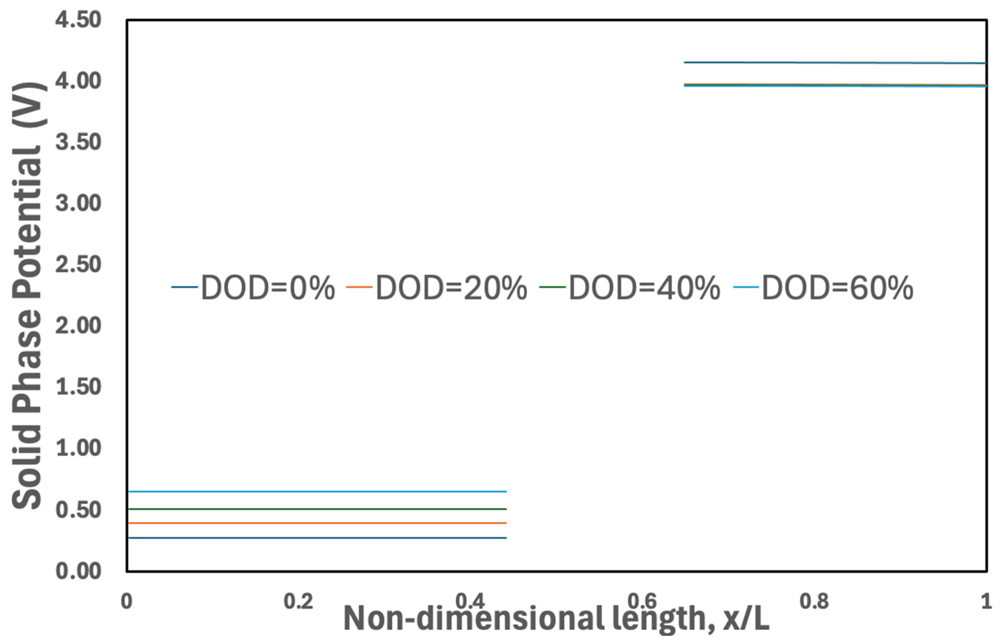
3.3.5. Solid-Phase Potential

Figure 21 demonstrates the variation of potential in both positive and negative electrodes for different DOD values at a discharge rate of 3 C. Initially, at a DOD = 0%, the potential of the negative electrode is nearly 0 V due to the high concentration of lithium ions present there. With an increasing DOD, as more lithium ions are removed, the negative electrode potential increases. The decreasing potential in the positive electrode with an increasing DOD value is brought about due to increasing lithium-ion concentrations. The decreasing lithium-ion surface concentrations in the negative electrode and the increasing lithium-ion surface concentrations in the positive electrode can be seen in Figure 17. A big difference in the electrical potential plots in Figure 21 and the surface lithium particle concentrations in Figure 17 is the slope of the curves. The electric potentials are flat while the surface concentration plots have significant slopes to them. Flat electrical potentials in the electrodes are driven by high electrical conductivities, relative to the electrode thickness. The surface particle concentrations adjust to provide flat electric potential profiles and thus have much larger changes.

3.3.6. Overpotential

The overpotential is the voltage difference between the active particle and the electrolyte that surrounds it. Overpotentials are needed to drive lithium ions out or into the active particles. A positive overpotential is used to drive lithium ions out of the active particles in the negative electrode and a negative overpotential is used to drive ions into the active particles in the positive electrodes. At times, depending on surface lithium-ion concentrations along the electrode, the overpotentials at some locations in the electrode can be the opposite of what is expected. The electrode overpotential can be the sum of three different components: activation overpotential, ohmic overpotential and concentration overpotential. Ohmic overpotentials arise due to a flow resistance of ions from the active particles to the surrounding electrolyte, activation overpotential is due to reaction activation energy and concentration overpotential is due to the difference in the ion concentration at an electrode–electrolyte interface. Therefore, the overpotential represents losses in the battery caused by transport and kinetic limitations.

In Figure 22, the overpotential is observed to decrease with an increasing DOD at the negative electrode, while increasing with increasing DOD values at the positive electrode. This happens to aid the transfer of lithium particles between the electrolyte and the active particles as the concentrations change. The higher overpotential value observed at the electrode–electrolyte interface for a DOD value of 0% arises due to the high lithium-ion concentration gradient between the electrode and electrolyte at the start of the discharging process. The overpotential changes as the DOD increases because the concentration gradient between the active particles and the electrolyte changes with DOD.

4. Conclusions

This work presented a comprehensive electrochemical–thermal model for simulating the operating behavior of a lithium-ion battery, designed to capture the interaction between electrical, chemical and thermal effects for both dynamic and static current operating conditions. A coupled set of partial differential equations are solved with the aid of a finite volume numerical technique implemented in a MATLAB computer code. Particle concentrations, electrical potentials and temperature profiles as a function of time and position within the negative electrode, the separator and the positive electrode are outputs of the computer model. The model presented in this research work built upon the work of Borakhadikar [11] by making some adjustments to the electrochemical model and adding a thermal model to the MATLAB computer code. At this point the code can couple thermal considerations of the battery behavior with electrochemical considerations.

The results obtained with the electrochemical–thermal model presented here were validated against those of Smith and Wang [13] and Gu and Wang [20]. Comparisons of the electrochemical results for static current inputs in the discharge and charging modes were excellent. For dynamic current inputs of a pulsed nature that are typical of a hybrid electrical vehicle application, the comparisons were good. In general, the static and dynamic electrochemical results from this work were within about 3% of the results presented by Smith and Wang. To achieve these comparisons, a correction was made to the negative electrode thickness of Smith and Wang, who stated a negative electrode thickness that did not correlate with their stated ampere hour capacity of the battery. Before making this change, results from this work showed battery voltages falling off sooner than those of Smith and Wang. The thermal model of this work was validated against the results published by Gu and Wang. The observed difference in the results produced by this work and those produced by Gu and Wang was largely because Gu and Wang used a lumped modeling approach, whereas a spatially distributed approach was used in this work, as described in Section 3. A distributed approach is more physically realistic. When this work used thermal source terms like those published by Gu and Wang, the comparisons were good. These comparisons validate all of the thermal model except the source term portion and also show the effect of using a distributed source term model compared to a lumped source term model.

A few aspects of the thermal behavior of a lithium-ion battery cell were studied. First, the effect of temperature-dependent properties was considered. Including temperature-dependent properties, instead of keeping them constant at their 25 °C value, had significant effects on the battery voltage and the operation temperature of the battery. Using temperature-dependent properties increased cell voltages and reduced operating temperatures over all DODs. Thus, an improved performance occurs because of the improved material properties in the battery with temperature increases. Plots showing how some of the material properties important to lithium-ion battery operation increase with temperature were presented.

For one operating current of 3 C, for a small battery cell, the spatial profiles of the temperature, lithium particle concentrations at the surface of the active particles, lithium particle concentrations in the active particles, lithium particle concentrations in the electrolyte and overpotentials were presented. It is interesting that the temperature profile across a battery cell is essentially uniform at any given time of operation. The temperature increases as current is continually released from the battery, but does so with a uniform profile across the negative electrode, the separator and the positive electrode. The lithium-ion concentrations in the cell set up to deliver the load current, that is, the concentrations within the active particles, the active particle surface concentrations within the metal electrodes and the concentrations in the electrolyte. The overpotentials adjust to make this happen.

References

1. Gong, Q.; Wang, P.; Cheng, Z. A novel deep neural network model for estimating the state of charge of lithium-ion battery. J. Energy Storage 2022, 54, 105308. [Google Scholar] [CrossRef]
2. Pillai, P.; Sundaresan, S.; Kumar, P.; Pattipati, K.R.; Balasingam, B. Open-Circuit Voltage Models for Battery Management Systems: A Review. Energies 2022, 15, 6803. [Google Scholar] [CrossRef]
3. Tran, M.K.; Mathew, M.; Janhunen, S.; Panchal, S.; Raahemifar, K.; Fraser, R.; Fowler, M. A comprehensive equivalent circuit model for lithium-ion batteries, incorporating the effects of state of health, state of charge, and temperature on model parameters. J. Energy Storage 2021, 43, 103252. [Google Scholar]
4. De Angelis, A.; Carbone, P.; Santoni, F.; Vitelli, M.; Ruscitti, L. On the Usage of Battery Equivalent Series Resistance for Shuntless Coulomb Counting and SOC Estimation. Batteries 2023, 9, 286. [Google Scholar] [CrossRef]
5. Abaspour, M.; Pattipati, K.R.; Shahrrava, B.; Balasingam, B. Robust Approach to Battery Equivalent-Circuit-Model Parameter Extraction Using Electrochemical Impedance Spectroscopy. Energies 2022, 15, 9251. [Google Scholar] [CrossRef]
6. Newman, J.; Tobias, C.W. Theoretical Analysis of Current Distribution in Porous Electrodes. J. Electrochem. Soc. 1962, 109, 1183–1191. [Google Scholar]
7. Doyle, M.; Fuller, T.F.; Newman, J. Modeling of Galvanostatic Charge and Discharge of the Lithium/Polymer/Insertion Cell. J. Electrochem. Soc. 1993, 140, 1526–1533. [Google Scholar] [CrossRef]
8. Moura, S.J.; Argomedo, F.B.; Klein, R.; Mirtabatabaei, A.; Krstic, M. Battery State Estimation for a Single Particle Model With Electrolyte Dynamics. IEEE Trans. Control Syst. Technol. 2017, 25, 453–468. [Google Scholar] [CrossRef]
9. Ma, Y.; Yin, M.; Ying, Z.; Chen, H. Establishment and simulation of an electrode averaged model for a lithium-ion battery based on kinetic reactions. RSC Adv. 2016, 6, 25435–25443. [Google Scholar] [CrossRef]
10. Santhanagopalan, S.; Guo, Q.; Ramadass, P.; White, R.E. Review of models for predicting the cycling performance of lithium ion batteries. J. Power Sources 2006, 156, 620–628. [Google Scholar]
11. Borakhadikar, A.S. One Dimensional Computer Modeling of a Lithium-Ion Battery. Master’s Thesis, Department of Mechanical and Materials Engineering, Wright State University, Dayton, OH, USA, 2017. Available online: http://rave.ohiolink.edu/etdc/view?acc_num=wright1496056104287962 (accessed on 6 January 2022).
12. Smith, K.A.; Rahn, C.D.; Wang, C.-Y. Control oriented 1D electrochemical model of lithium ion battery. Energy Convers. Manag. 2007, 48, 2565–2578. [Google Scholar] [CrossRef]
13. Smith, K.; Wang, C.Y. Solid-state diffusion limitations on pulse operation of a lithium-ion cell for hybrid electric vehicles. J. Power Sources 2006, 165, 678–686. [Google Scholar] [CrossRef]
14. Białoń, T.; Niestrój, R.; Skarka, W.; Korski, W. HPPC Test Methodology Using LFP Battery Cell Identification Tests as an Example. Energies 2023, 16, 6239. [Google Scholar] [CrossRef]
15. Rotas, R.; Iliadis, P.; Nikolopoulos, N.; Rakopoulos, D.; Tomboulides, A. Dynamic Battery Modeling for Electric Vehicle Applications. Batteries 2024, 10, 188. [Google Scholar] [CrossRef]
16. Katrašnik, T.; Mele, I.; Zelič, K. Multi-scale modelling of Lithium-ion batteries: From transport phenomena to the outbreak of thermal runaway. Energy Convers. Manag. 2021, 236, 114036. [Google Scholar] [CrossRef]
17. Kim, Y.; Mohan, S.; Siegel, J.B.; Stefanopoulou, A.G.; Ding, Y. The Estimation of Temperature Distribution in Cylindrical Battery Cells Under Unknown Cooling Conditions. IEEE Trans. Control Syst. Technol. 2014, 22, 2277–2286. [Google Scholar]
18. Li, Y.; Wei, Z.; Xiong, B.; Vilathgamuwa, D.M. Adaptive Ensemble-Based Electrochemical-Thermal Degradation State Estimation of Lithium-Ion Batteries. IEEE Trans. Ind. Electron. 2022, 69, 6984–6996. [Google Scholar]
19. Chiew, J.; Chin, C.S.; Toh, W.D.; Zhang, C. A pseudo three-dimensional electrochemical-thermal model of a cylindrical LiFePO4/graphite battery. Appl. Therm. Eng. 2018, 147, 106. [Google Scholar] [CrossRef]
20. Gu, W.B.; Wang, C.Y. Thermal and electrochemical coupled modeling of a lithium-ion cell. J. Power Sources 2000, 99, 25–37. [Google Scholar]
21. Patankar, S.V. Numerical Heat Transfer and Fluid Flow; Hemisphere: New York, NY, USA, 1980. [Google Scholar]
22. Sun, J.; Kainz, J. Optimization of hybrid pulse power characterization profile for equivalent circuit model parameter identification of Li-ion battery based on Taguchi method. J. Energy Storage 2023, 70, 108034. [Google Scholar] [CrossRef]
Figure 1. Computational domain showing the volume discretization using the finite volume method.
Energies 18 01764 g001
Figure 2. Flow chart detailing program execution steps.
Energies 18 01764 g002
Figure 3. Comparisons of cell voltages from the results of Smith and Wang [13] and the results from the computer program developed as part of this work for a static current load of 1 C.
Energies 18 01764 g003
Figure 4. Charge–discharge current pulses for HPPC current profile.
Energies 18 01764 g004
Figure 5. Validation of program voltage response versus Smith and Wang [13] for a dynamic current profile.
Energies 18 01764 g005
Figure 6. Coupled and decoupled cell voltage comparisons with Gu and Wang [20], of 3 C discharge and h = 0 W/m2-K to the coupled results of Gu and Wang [20].
Energies 18 01764 g006
Figure 7. Decoupled and coupled cell temperature comparisons with Gu and Wang [20], for a 3 C discharge and h = 0 W/m2-K.
Energies 18 01764 g007
Figure 8. Comparison of the adjusted decoupled cell temperature results from this work for a 3 C discharge and h = 0 W/m2-K to the decoupled results of Gu and Wang [20].
Energies 18 01764 g008
Figure 9. Comparison of the adjusted coupled cell temperature results from this work for a 3 C discharge and h = 0 W/m2-K to the coupled results of Gu and Wang [20].
Energies 18 01764 g009
Figure 10. Effect of C-rates on battery cell average temperatures for h = 0 W/m2-K.
Energies 18 01764 g010
Figure 11. Effect of boundary heat transfer coefficient on battery cell temperatures for a discharge current load of 3 C.
Energies 18 01764 g011
Figure 12. Exchange current density variation with temperature.
Energies 18 01764 g012
Figure 13. Change in diffusivity in the active particles at the positive and negative electrodes with temperature.
Energies 18 01764 g013
Figure 14. Change in diffusivity of the electrolyte phase with temperature.
Energies 18 01764 g014
Figure 15. Change in electrolyte conductivity with temperature.
Energies 18 01764 g015
Figure 16. Cell temperatures for different DOD values, for a 3 C discharge rate and h = 0 W/m2-K.
Energies 18 01764 g016
Figure 17. Solid-phase surface concentration of lithium ions for different DOD values, for a 3 C discharge rate and h = 0 W/m2-K.
Energies 18 01764 g017
Figure 18. Concentration of lithium particles in the active spherical particles located in the middle of the negative electrode for different DOD values, for a 3 C discharge rate and h = 0 W/m2-K.
Energies 18 01764 g018
Figure 19. Lithium particle concentration in the active spherical particles located in the middle of the positive electrode for different DOD values, for a 3 C discharge rate and h = 0 W/m2-K.
Energies 18 01764 g019
Figure 20. Electrolyte lithium-ion concentration for different DOD values, for a 3 C discharge rate and h = 0 W/m2-K.
Energies 18 01764 g020
Figure 21. Solid potential across electrodes for different DOD values, for a 3 C discharge rate and h = 0 W/m2-K.
Energies 18 01764 g021
Figure 22. Overpotentials in electrodes for different DOD values, for a 3 C discharge rate and h = 0 W/m2-K.
Energies 18 01764 g022