PEMFC Semi-Empirical Model Improvement by Reconstructing Concentration Loss

Abstract

The performance of proton exchange membrane fuel cells (PEMFCs) is greatly affected by their operating parameters, especially at high current densities. An advanced concentration loss model is proposed to improve a semi-empirical model describing PEMFC polarization, with the aim of accurate prediction at the whole current density interval from low to high levels. Experiments are designed to verify the improved semi-empirical model. Model comparison shows that the improved semi-empirical model has a better prediction accuracy and generalization ability than others. The effects of operating parameters and structural parameters on PEMFC performance are analyzed. The results indicate that a relatively high operating temperature, pressure, and gas diffusion layer (GDL) porosity can increase PEMFC performance. The influence of relative humidity and PEM thickness on PEMFC performance is different at low and high current densities. A relatively high humidity can improve PEMFC performance at a low current density, but PEMFC performance will be reduced if the relative humidity is too high at a high current density. A thinner PEM thickness can improve PEMFC performance at a low current density, but PEMFC performance does not necessarily improve with a decreasing PEM thickness at a high current density. Overall, the improved semi-empirical model realizes an accurate analysis of PEMFC performance from a low to high current density.

1. Introduction

The scarcity of fossil fuels and environmental pollution have accelerated the exploration of new energy sources. Fuel cells have attracted the attention of researchers due to their simple structure and low pollution [1,2,3]. Among different types of fuel cells, PEMFCs have been widely recognized as the most effective power generation device for the future, benefiting from advantages such as a low operating temperature, high power density, and flexible size [4,5,6].

Improving power density is vital for the development of fuel cell vehicles (FCVs). According to state-of-the-art FCV products and worldwide fuel cell programs, the working current density and cell voltage is expected to increase to 3–4 A cm⁻² and 0.7–0.8 V in the next decade, respectively [7]. However, concentration loss becomes a major factor reducing PEMFC performance at a high current density, which is contrary to the future goal of maintaining a high output voltage at a high working current density. Therefore, much work has been conducted to reduce concentration loss and improve PEMFC performance at a high current density, such as modifications of catalyst material [8,9,10], the optimization of the flow field [11,12,13], and the structure improvement of the membrane electrode assembly (MEA) [14,15,16]. Besides improvements in material and structure, appropriate operating parameters are also essential for PEMFCs to maintain a stable performance at high current densities. Therefore, a good understanding and accurate modeling of PEMFC behavior at a high current density are necessary to guide the optimization of operating parameters. Up until now, the modeling of concentration loss has received the attention from researchers, and some models have been proposed. O’hayre et al. [17] constructed a concentration loss mechanism model by considering the mass transfer loss of reactants in the flow channel and GDL. Abdin et al. [18] proposed a concentration loss model by emphatically considering the transport of anode and cathode gas and the across-membrane transport of water. The model emulated experimental data well, especially at a high current density. Hasegawa et al. [19] formulated a fuel cell polarization model by constructing a new mass transport model. The model was validated and verified with experimental data collected from the commercial fuel cell system of a second-generation Miral. Strong agreements were confirmed between the experimental data and the simulation results.

Based on the above references, it can be found that existing models can describe fuel cell performance at a high current density. However, water phase changes and the effect of liquid water on GDL porosity, which have been proven to have a great influence on fuel cell performance under a large current density, were ignored in the above concentration loss modeling processes [20,21,22]. Due to the lack of descriptions of important physical phenomena, the above concentration loss models cannot fully capture the influence of physical parameters on PEMFC performance, which is unfavorable for guiding PEMFCs to work at high current densities. In this paper, an advanced concentration loss model is proposed, then the semi-empirical model describing PEMFC polarization is further developed. This model is distinguished from other PEMFC models by the following. (i) Physically meaningful parameters are kept in the model, so the model can be used to estimate the values of physical parameters that are difficult to obtain directly through experiments. (ii) Calculation methods for the same parameters in different structures are introduced, so the model can be widely used in PEMFCs with different component structures. (iii) Multiple physical phenomena are considered during the modeling, including the convection and diffusion transport of reactant gas, the phase changes and across-membrane transport of water, and dynamic changes in GDL porosity. The correctness and generalization ability of the semi-empirical model are verified by an orthogonal experiment. Based on the model, the influence of operating parameters and component structural parameters on PEMFC performance is explored, and applications in optimizing operating parameters and solving physical coefficients are prospected. Such research will facilitate a deeper understanding of PEMFC working mechanisms and lay a foundation for the optimization of operating parameters under a high current density in the future.

2. Model Development

The semi-empirical model has been developed based on the following simplified assumptions, without losing essential contributions to the cell performance.

(1)

The PEMFC operates under a steady-state condition, and any transient phenomena are not included in this model.

(2)

The anode, cathode, and membrane are at the same temperature.

(3)

In the PEMFC, oxygen reduction is dominant because it is much slower than hydrogen oxidation. Therefore, the activation loss and concentration loss of the anode are ignored in the modeling.

(4)

The reactants are pure hydrogen and air, which are regarded as ideal gases.

(5)

The GDLs, catalyst layers, and membrane are treated as isotropic porous media.

(6)

The PEM is not electrically conductive and is impermeable to neutral reactant gases, so internal currents and fuel crossover losses are not considered.

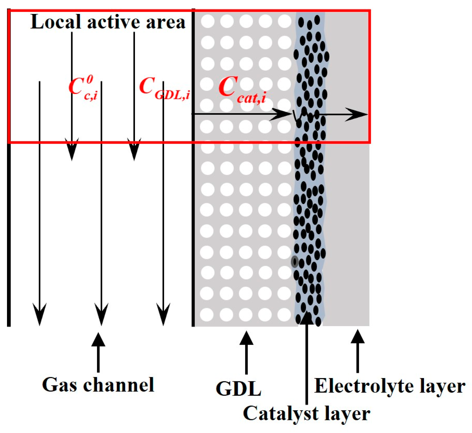
2.1. Concentration Loss

Concentration loss occurs when the reactants in the electrochemical reaction form a concentration gradient. The concentration gradient is caused by two basic transport obstacles. Firstly, the reactant gas is hindered by the GDL when it diffuses from the flow channel to the catalyst surface. Secondly, the water produced from the reaction can occupy the pores of GDL and then obstruct the reactant gas transport. Therefore, revealing the gas transport and water transport processes is the key to reconstructing the concentration loss model.

2.1.1. Gas Transport

As shown in Figure 1, the cathode reactant gas in each local active area reaches the catalyst layer through convection transport in the flow channel and diffusion transport in the GDL when the PEMFC operates steadily. This process can be expressed by convection transport and the Fick diffusion law as follows [23]:

$$J=A_i{h}_{\mathrm{m},i}\left(C_{\mathrm{c},i}^0-C_{\mathrm{GDL},i}\right)$$

(1)

$$J=A_i{D}_{ij,i}^{\mathrm{eff}}{\displaystyle \frac{C_{\mathrm{GDL},i}-C_{\mathrm{cat},i}}{L_{\mathrm{GDL}}}}$$

(2)

The current is generated when the reactants on the catalyst surface participate in electrochemical reactions. This process can be expressed by the Faraday law, as follows [17]:

$$i={\displaystyle \frac{nFJ}{A_i}}$$

(3)

A dynamic balance state is reached between the gas transport in the components and gas consumption in the catalyst layer. The current generated in each local active area can be calculated by combining Equations (1)–(3), as follows:

$$i=nF{\displaystyle \frac{C_{\mathrm{c},i}^0-C_{\mathrm{cat},i}}{\frac{1}{h_{\mathrm{m},i}}+\frac{L_{\mathrm{GDL}}}{D_{ij,i}^{\mathrm{eff}}}}}$$

(4)

For each reaction area below the flow channel, a limiting current density ($i_{\mathrm{L}}$) occurs when the current density becomes so large that the reactant concentration on the catalyst surface falls to zero. For single cell, the limiting current density ($i_{\mathrm{L}}$) can be calculated by the average of the sum of the local limiting current densities ($i_{\mathrm{L}}$), as follows:

$$i_{\mathrm{L}}={\displaystyle \frac{{\displaystyle \sum _{i=1}^N{i}_{\mathrm{L},i}}}{N}}={\displaystyle \frac{{\displaystyle \sum _{i=1}^N\left(nF\frac{C_{\mathrm{c},i}^0}{\frac{1}{h_{\mathrm{m},i}}+\frac{L_{\mathrm{GDL}}}{D_{ij,i}^{\mathrm{eff}}}}\right)}}{N}}=nF{\displaystyle \frac{C_{\mathrm{c}}^0}{\frac{1}{h_{\mathrm{m}}}+\frac{L_{\mathrm{GDL}}}{D_{ij}^{\mathrm{eff}}}}}$$

(5)

where $J$ is the mass transfer rate (mol s⁻¹); $A_i$ is the local active area of MEA (cm²); $C_{\mathrm{c},i}^0$, $C_{\mathrm{GDL},i}$, and $C_{\mathrm{cat},i}$ are the concentrations of the reactant at the local cathode channel, GDL surface, and catalyst surface, respectively (mol cm⁻³); $C_{\mathrm{c}}^0$ is the average concentration of reactant in the flow channel; $h_{\mathrm{m},i}$ and $h_{\mathrm{m}}$ are the local and global convection mass transfer coefficients, respectively (cm s⁻¹); $L_{\mathrm{GDL}}$ is the thickness of the GDL (cm); $D_{ij,i}^{\mathrm{eff}}$ and $D_{ij}^{\mathrm{eff}}$ are the local and global effective diffusion coefficients for the GDL (cm² s⁻¹); $i$ is the current density (A cm⁻²); n is the number of electrons consumed in the reaction (n = 4); and $F$ is the Faraday constant (F = 96,485 C mol⁻¹).

$C_{\mathrm{c}}^0$ can be calculated by the following [11]:

$$C_{\mathrm{c}}^0={\displaystyle \frac{\left(P_{\mathrm{c},\mathrm{in}}-R{H}_{\mathrm{c},\mathrm{in}}{P}_{\mathrm{sat}\left({\mathrm{T}}_{\mathrm{c},\mathrm{in}}\right)}\right)\times \mathrm{101,325}\times r_{{\mathrm{O}}_2,\mathrm{in}}}{R\times T_{\mathrm{c},\mathrm{in}}\times \mathrm{1,000,000}}}$$

(6)

where $P_{\mathrm{c},\mathrm{in}}$ is the gas pressure at the cathode inlet (atm); $r_{{\mathrm{O}}_2,\mathrm{in}}$ is the volume fraction of oxygen at the cathode inlet; $R{H}_{\mathrm{c},\mathrm{in}}$ is the gas humidity of the cathode inlet; $R$ is the ideal gas constant (8.314 J mol⁻¹ K⁻¹ or 8.314 m³ Pa mol⁻¹ K⁻¹); $T_{\mathrm{c},\mathrm{in}}$ is the gas temperature of the cathode inlet (K); and $P_{\mathrm{sat}\left({\mathrm{T}}_{\mathrm{c},\mathrm{in}}\right)}$ is the saturation pressure of the water at the cathode inlet (atm). $P_{\mathrm{sat}}$ can be calculated as follows [23]:

$$\log \left(P_{\mathrm{sat}}\right)=2.95\times {10}^{-2}\left(T-273.15\right)-9.19\times {10}^{-5}{\left(T-273.15\right)}^2+1.44\times {10}^{-7}{\left(T-273.15\right)}^3-2.18$$

(7)

Through the above modeling, the gas transport in the local area below the flow channel is extended to the whole flow field. In this study, $h_{\mathrm{m}}$ represents the mass transfer ability of the entire flow field. The value of $h_{\mathrm{m}}$ is dependent upon the wall condition, the channel geometry, and the physical properties of the input gas [17,23]. $h_{\mathrm{m}}$ is determined by the Sherwood number ($Sh$), as follows:

$$h_{\mathrm{m}}=Sh{\displaystyle \frac{D_{ij}}{d}}$$

(8)

where $D_{ij}$ is the effective binary diffusion coefficient for species i and j (cm² s⁻¹) and $d$ is the characteristic length of flow channel. For equal section channels, $d$ is calculated by four times the ratio of the section area to the channel circumference, and for non-equal section channels, $d$ is calculated by the ratio of the volume to the channel surface area.

Many studies have found that Sherwood numbers are related to Schmidt numbers ($Sc$) and Reynolds numbers ($Re$) [24,25]. By summarizing previous studies, the relationship between them can be generally expressed as follows:

$$Sh=a{\left(Sc\right)}^b{\left(Re\right)}^c$$

(9)

where a, b, and c are constants, which can be obtained by experiments.

The following equations were used to calculate $Sc$ and $Re$ [17,26,27,28]:

$$Sc={\displaystyle \frac{{\mu }_{\mathrm{mix}}}{\rho D_{ij}}}$$

(10)

$$Re={\displaystyle \frac{du\rho }{{\mu }_{\mathrm{mix}}}}$$

(11)

$${\mu }_{\mathrm{mix}}={\displaystyle \sum _{i=1}^N\frac{x_i{\mu }_i}{{\displaystyle {\sum }_{j=1}^N{x}_j{\Phi }_{ij}}}}$$

(12)

$${\mu }_i={\mu }_{i,0}\left({\displaystyle \frac{T_0+C}{T_{\mathrm{c},\mathrm{in}}+C}}\right){\left({\displaystyle \frac{T_{\mathrm{c},\mathrm{in}}}{T_0}}\right)}^{1.5}$$

(13)

$${\Phi }_{ij}={\displaystyle \frac{1}{\sqrt{8}}}{\left(1+{\displaystyle \frac{M_i}{M_j}}\right)}^{-0.5}{\left(1+{\left({\displaystyle \frac{{\mu }_i}{{\mu }_j}}\right)}^{0.5}{\left({\displaystyle \frac{M_i}{M_j}}\right)}^{0.25}\right)}^2$$

(14)

$$\rho ={\displaystyle \frac{101.325\times \left(\left(P_{\mathrm{c},\mathrm{in}}-P_{\mathrm{sat}\left({\mathrm{T}}_{\mathrm{c},\mathrm{in}}\right)}\right)M_{\mathrm{air}}+P_{\mathrm{sat}\left({\mathrm{T}}_{\mathrm{c},\mathrm{in}}\right)}{M}_{{\mathrm{H}}_2\mathrm{O}}\right)}{R\times 1000\times T_{\mathrm{c},\mathrm{in}}}}$$

(15)

$$u={\displaystyle \frac{Z_{\mathrm{air},\mathrm{in}}}{N_{\mathrm{cell}}{N}_{\mathrm{ch}}{A}_{\mathrm{ch}}}}$$

(16)

$$Z_{\mathrm{air},\mathrm{in}}={\displaystyle \frac{I}{4F}}{\displaystyle \frac{S_{{\mathrm{O}}_2}}{r_{{\mathrm{O}}_2,\mathrm{in}}}}{\displaystyle \frac{R{T}_{\mathrm{c},\mathrm{in}}}{P_{\mathrm{c},\mathrm{in}}-R{H}_{\mathrm{c},\mathrm{in}}{P}_{\mathrm{sat}\left({\mathrm{T}}_{\mathrm{c},\mathrm{in}}\right)}}}{N}_{\mathrm{cell}}\times {10}^6$$

(17)

where ${\mu }_{\mathrm{mix}}$, $\rho$, and $u$ are the viscosity (g cm⁻¹ s⁻¹), density (g cm⁻³), and flow rate (cm s⁻¹) of the mixed gas, respectively; ${\mu }_i$ is the gas viscosity of species i; and ${\mu }_{\mathrm{i},0}$ is the corresponding viscosity of species i at the reference temperature $T_0$, which can be found in

Table 1. The viscosity of different substances [17].

Gas	${\mathit{\mu }}_{\mathit{i},0}\left(10^{-5}\mathbf{g}/\mathbf{c}\mathbf{m}\cdot \mathbf{s}\right)$	${\mathit{T}}_0\left(\mathbf{K}\right)$	C
Air	17.16	273	111
N2	16.63	273	107
O2	19.19	273	139
H2	8.411	273	47
H2O	11.2	350	1064

. ${\Phi }_{ij}$ is the dimensionless number; $M_{\mathrm{air}}$ and $M_{{\mathrm{H}}_2\mathrm{O}}$ are the molar masses of air and water (g mol⁻¹); $N_{\mathrm{cell}}$ is the number of single cells in the stack; $N_{\mathrm{ch}}$ is the number of parallel flow channels in each single cell; $A_{\mathrm{ch}}$ is the cross-sectional area of flow channels (cm²); $Z_{\mathrm{air},\mathrm{in}}$ is the total flow at the PEMFC cathode inlet (cm³ s⁻¹); $I$ is the current (A); and $S_{{\mathrm{O}}_2}$ is the stoichiometric ratio of oxygen;

$D_{ij}^{\mathrm{eff}}$ in Equation (5) is related to $D_{ij}$ in Equation (8). $D_{ij}$ and $D_{ij}^{\mathrm{eff}}$ can be calculated as follows [29]:

$$D_{ij}=D_{ij,0}{\displaystyle \frac{P_0}{P_{\mathrm{c},\mathrm{in}}}}{\left({\displaystyle \frac{T_{\mathrm{c},\mathrm{in}}}{T_0}}\right)}^{1.5}$$

(18)

$$D_{ij}^{\mathrm{eff}}=D_{ij}{\epsilon }^{1.5}$$

(19)

where $D_{ij,0}$ is the binary diffusion coefficient for substances i and j at the reference temperature $T_0$ and reference pressure $P_0$ and the values of different species are shown in

Table 2. The binary diffusion coefficients for different substances at 1 standard atmosphere [23].

Substance i	Substance j	${\mathit{T}}_0\left(\mathbf{K}\right)$	${\mathit{D}}_{\mathit{i}\mathit{j},0}\left(\mathbf{c}{\mathbf{m}}^2/\mathbf{s}\right)$
H2	H2O	298	$0.63\times {10}^{-4}$
O2	H2O	298	$0.24\times {10}^{-4}$
O2	N2	273	$0.18$
N2	H2O	298	$0.26\times {10}^{-4}$

. $\epsilon$ is the effective porosity of GDL, which is greatly affected by the liquid water and can be calculated by the following [20,30]:

$$\epsilon ={\epsilon }_0\left(1-{\displaystyle \frac{y_{\mathrm{l}}}{y_{\mathrm{GDL}}}}\right)$$

(20)

where ${\epsilon }_0$ is the initial porosity, $y_{\mathrm{l}}$ is the volume of liquid water in the GDL (L), and $y_{\mathrm{GDL}}$ is the volume of pores in the GDL (L).

In actual calculations, $y_{\mathrm{l}}$ is difficult to estimate. Therefore, Equation (20) is changed as follows to facilitate the calculation:

$$\epsilon ={\epsilon }_0\left(1-{\displaystyle \frac{y_{\mathrm{l}}}{y_{\mathrm{GDL}}}}\right)={\epsilon }_0\left(1-{\displaystyle \frac{\frac{y_{\mathrm{l}} \times M_{{\mathrm{H}}_2\mathrm{O}}}{t \times 22.4}}{\frac{y_{\mathrm{GDL}} \times M_{{\mathrm{H}}_2\mathrm{O}}}{t \times 22.4}}}\right)={\epsilon }_0\left(1-{\displaystyle \frac{Y_{\mathrm{l}}}{Y_{\mathrm{GDL}}}}\right)$$

(21)

where t is time (s); $Y_{\mathrm{GDL}}$ is the flow of liquid water corresponding to complete flooding (g s⁻¹); and $Y_{\mathrm{l}}$ is the flow of liquid water in the membrane corresponding to the water balance (g s⁻¹), which can be calculated from the water transport inside the PEMFC.

2.1.2. Water Transport

Figure 2 describes the water transport inside the PEMFC. The following equation was used to express the water transport relationship [18,23]:

$$Y_{\mathrm{c},\mathrm{out}}=Y_{\mathrm{c},\mathrm{in}}+Y_{\mathrm{c},\mathrm{gen}}+\left(Y_{\mathrm{c},\mathrm{ed}}-Y_{\mathrm{c},\mathrm{bd}}-Y_{\mathrm{c},\mathrm{hp}}-Y_{\mathrm{c},\mathrm{te}}\right)$$

(22)

where $Y_{\mathrm{c},\mathrm{out}}$ is the flow of water discharged from the cathode outlet (g s⁻¹); $Y_{\mathrm{c},\mathrm{in}}$ is the amount of water injected into the cathode with the fuel (g s⁻¹); $Y_{\mathrm{c},\mathrm{gen}}$ is the amount of water produced by the chemical reaction (g s⁻¹); $Y_{\mathrm{c},\mathrm{ed}}$ is the mass flow rate due to electro-osmotic drag (g s⁻¹); $Y_{\mathrm{c},\mathrm{bd}}$ is the back diffusion (g s⁻¹); $Y_{\mathrm{c},\mathrm{hp}}$ is the hydraulic permeation due to pressure difference (g s⁻¹); and $Y_{\mathrm{c},\mathrm{te}}$ is the thermos-osmosis due to temperature difference (g s⁻¹).

The relationship between $Y_{\mathrm{c},\mathrm{ed}}$, $Y_{\mathrm{c},\mathrm{bd}}$, $Y_{\mathrm{c},\mathrm{hp}}$, and $Y_{\mathrm{c},\mathrm{te}}$ represents the net water transported across the membrane, The following equations were used to calculate $Y_{\mathrm{c},\mathrm{in}}$, $Y_{\mathrm{c},\mathrm{ed}}$, $Y_{\mathrm{c},\mathrm{gen}}$, and $Y_{\mathrm{c},\mathrm{bd}}$ [18,23,27,28,31,32,33,34,35]:

$$Y_{\mathrm{c},\mathrm{in}}={\displaystyle \frac{S_{{\mathrm{O}}_2}}{r_{{\mathrm{O}}_2}}}{\displaystyle \frac{M_{{\mathrm{H}}_2\mathrm{O}}}{4F}}{\displaystyle \frac{R{H}_{\mathrm{c},\mathrm{in}}{P}_{\mathrm{sat}\left({\mathrm{T}}_{\mathrm{c},\mathrm{in}}\right)}}{P_{\mathrm{c},\mathrm{in}}-R{H}_{\mathrm{c},\mathrm{in}}{P}_{\mathrm{sat}\left({\mathrm{T}}_{\mathrm{c},\mathrm{in}}\right)}}}I$$

(23)

$$Y_{\mathrm{c},\mathrm{gen}}={\displaystyle \frac{M_{{\mathrm{H}}_2\mathrm{O}}}{2F}}I$$

(24)

$$Y_{\mathrm{c},\mathrm{ed}}=\left(0.0029{{\lambda }_{\mathrm{mem}}}^2+0.05{\lambda }_{\mathrm{mem}}-3.4\times {10}^{-19}\right){\displaystyle \frac{M_{{\mathrm{H}}_2\mathrm{O}}}{F}}I$$

(25)

$$Y_{\mathrm{c},\mathrm{bd}}=A{D}_{\mathrm{W}}{M}_{{\mathrm{H}}_2\mathrm{O}}{\displaystyle \frac{\left(C_{{\mathrm{H}}_2\mathrm{O},\mathrm{mem}}^{\mathrm{c}}-C_{{\mathrm{H}}_2\mathrm{O},\mathrm{mem}}^{\mathrm{a}}\right)}{L_{\mathrm{mem}}}}$$

(26)

$$D_{\mathrm{W}}=D_{\lambda }\exp \left(2416\left({\displaystyle \frac{1}{303}}-{\displaystyle \frac{1}{T}}\right)\right)$$

(27)

$$D_{\lambda }=\left\{\begin{array}{cc}{10}^{-6}& ,{\lambda }_{\mathrm{mem}}<2\\ {10}^{-6}\left(1+2\left({\lambda }_{\mathrm{mem}}-2\right)\right)& ,2\le {\lambda }_{\mathrm{mem}}\le 3\\ {10}^{-6}\left(3-1.67\left({\lambda }_{\mathrm{mem}}-3\right)\right)& ,3\le {\lambda }_{\mathrm{mem}}\le 4.5\\ 1.25\times {10}^{-6}& ,{\lambda }_{\mathrm{mem}}\ge 4.5\end{array}\right.$$

(28)

$$C_{{\mathrm{H}}_2\mathrm{O},\mathrm{mem}}^{\mathrm{c}}={\displaystyle \frac{{\rho }_{\mathrm{mem},\mathrm{dry}}}{M_{\mathrm{mem},\mathrm{dry}}}}{\lambda }_{\mathrm{c},\mathrm{in}}$$

(29)

$$C_{{\mathrm{H}}_2\mathrm{O},\mathrm{mem}}^{\mathrm{a}}={\displaystyle \frac{{\rho }_{\mathrm{mem},\mathrm{dry}}}{M_{\mathrm{mem},\mathrm{dry}}}}{\lambda }_{\mathrm{a},\mathrm{in}}$$

(30)

where $D_{\mathrm{W}}$ is the diffusion coefficient of water in the membrane (cm² s⁻¹); T is the cell temperature (K); $C_{{\mathrm{H}}_2\mathrm{O},\mathrm{mem}}^{\mathrm{c}}$ and $C_{{\mathrm{H}}_2\mathrm{O},\mathrm{mem}}^{\mathrm{a}}$ are the water concentrations at the cathode and anode sides of the membrane (mol cm⁻³); $L_{\mathrm{mem}}$ is the thickness of the membrane (cm); ${\rho }_{\mathrm{mem},\mathrm{dry}}$ is the density of the PEM when dry (g cm⁻³); $M_{\mathrm{mem},\mathrm{dry}}$ is the equivalent weight of the PEM when dry (g mol⁻¹); ${\lambda }_{\mathrm{mem}}$, ${\lambda }_{\mathrm{a},\mathrm{in}}$ and ${\lambda }_{c,in}$ are the water contents of the membrane, anode and cathode, respectively. The water content ${\lambda }_i$ is determined by the relative humidity $R{H}_i$ (subscript $i$ is either a, in-anode inlet, c, in-cathode inlet, or mem, membrane) [27].

$$\left\{\begin{array}{cc}{\lambda }_i=0.043+17.81R{H}_i-39.85R{H}_i^2+36R{H}_i^3\hfill & \hfill \mathrm{for} 0<R{H}_i\le 1\\ {\lambda }_i=14+1.4\left(R{H}_i-1\right)\hfill & \hfill \mathrm{for} 1<R{H}_i\le 3\end{array}\right.$$

(31)

where $R{H}_{\mathrm{mem}}$ is the humidity of the PEM, which is calculated from the average value of the humidity of the cathode and anode gases, as follows:

$$R{H}_{\mathrm{mem}}={\displaystyle \frac{R{H}_{\mathrm{a},\mathrm{in}}+R{H}_{\mathrm{c},\mathrm{in}}}{2}}$$

(32)

$Y_{\mathrm{c},\mathrm{hp}}$ is considered in the modeling because a proper pressure difference between the anode and cathode will improve PEMFC performance [36]. $Y_{\mathrm{c},\mathrm{te}}$ is not included in the analysis because this effect is obscured by the electro-osmotic drag and back diffusion. The mass flow rate of water due to hydraulic permeation can be calculated by the Darcy law, as follows:

$$Y_{\mathrm{c},\mathrm{hp}}={\displaystyle \frac{A{\rho }_{{\mathrm{H}}_2\mathrm{O}}{K}_{\mathrm{MEA}}}{{\mu }_{{\mathrm{H}}_2\mathrm{O}}}}{\displaystyle \frac{\left(P_{\mathrm{c},\mathrm{in}}-P_{\mathrm{a},\mathrm{in}}\right)\times \mathrm{1,013,250}}{L_{\mathrm{MEA}}}}$$

(33)

where ${\rho }_{{\mathrm{H}}_2\mathrm{O}}$ is the density of the water (g cm⁻³), $K_{\mathrm{MEA}}$ is the permeability of the MEA (cm²), and $L_{\mathrm{MEA}}$ is the thickness of the MEA (cm).

The water at the cathode outlet calculated according to Equation (22) represents water vapor. When the water vapor inside the fuel cell reaches the saturation state, it will condense in the form of liquid water. When liquid water is discharged from the cathode outlet, it means that liquid water has existed in the GDL already. The above relationship can be expressed as follows:

$$\left\{\begin{array}{cc}{Y}_{\mathrm{l}}=Y_{\mathrm{c},\mathrm{out}}-Y_{\mathrm{c},\mathrm{out},\mathrm{v}}& ,Y_{\mathrm{c},\mathrm{out}}>Y_{\mathrm{c},\mathrm{out},\mathrm{v}}\\ Y_{\mathrm{l}}=0& ,Y_{\mathrm{c},\mathrm{out}}\le Y_{\mathrm{c},\mathrm{out},\mathrm{v}}\end{array}\right.$$

(34)

where $Y_{\mathrm{c},\mathrm{out},\mathrm{v}}$ is the saturated water vapor flow at the cathode outlet. It can be expressed as follows [23]:

$$Y_{\mathrm{c},\mathrm{out},\mathrm{v}}={\displaystyle \frac{S_{{\mathrm{O}}_2}-r_{{\mathrm{O}}_2}}{r_{{\mathrm{O}}_2}}}{\displaystyle \frac{M_{{\mathrm{H}}_2\mathrm{O}}}{4F}}{\displaystyle \frac{P_{\mathrm{sat}\left({\mathrm{T}}_{\mathrm{c},\mathrm{out}}\right)}}{P_{\mathrm{c},\mathrm{out}}-P_{\mathrm{sat}\left({\mathrm{T}}_{\mathrm{c},\mathrm{out}}\right)}}}I$$

(35)

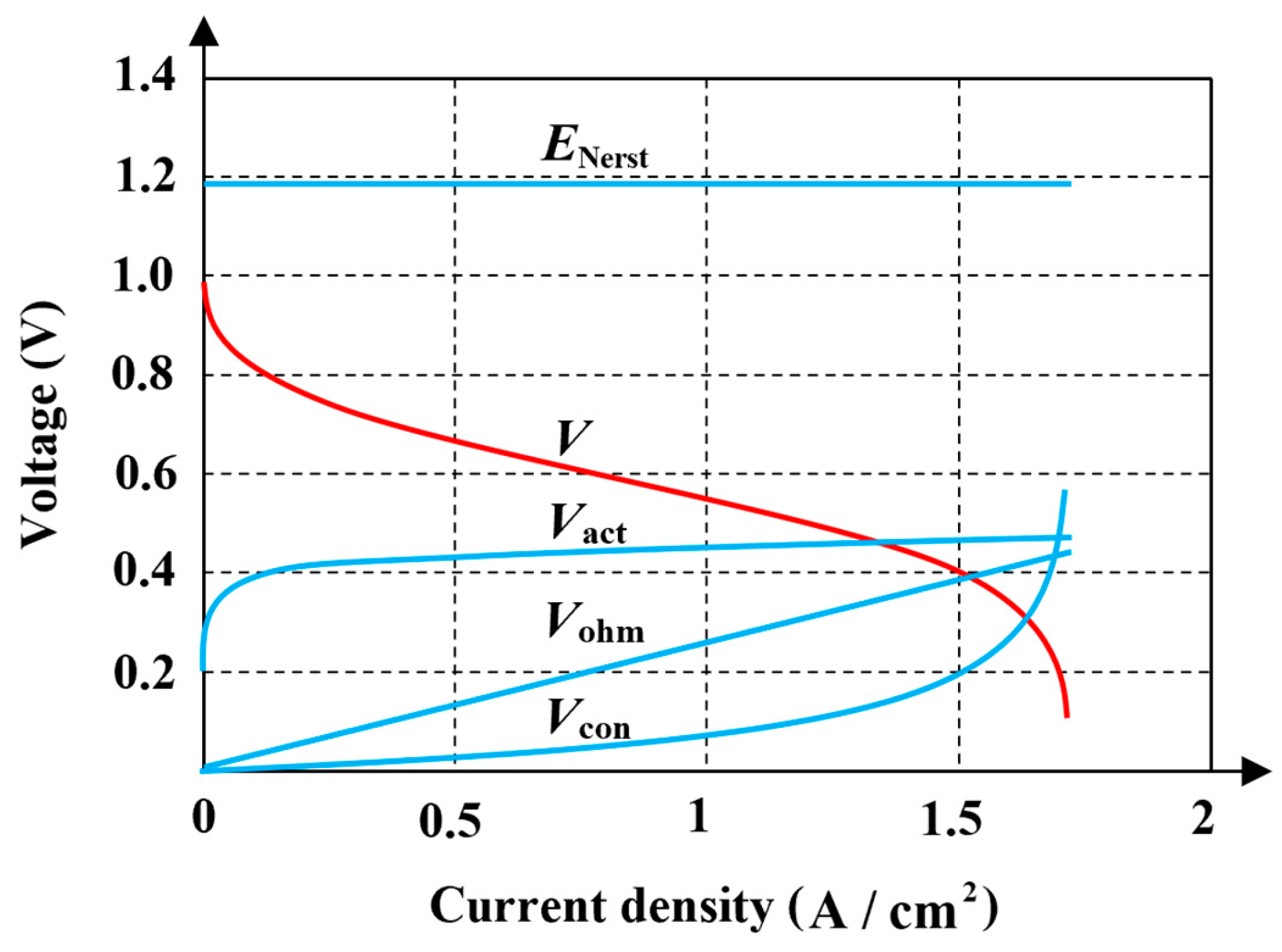
2.2. Semi-Empirical Model

The semi-empirical model in this research was developed based on the electrochemical reactions inside a PEMFC. As shown in Figure 3, the effect of electrochemical reactions on PEMFC performance can be graphically represented by the polarization curve. The cell voltage losses are composed of activation loss ($V_{\mathrm{act}}$), ohmic loss ($V_{\mathrm{ohm}}$), and concentration loss ($V_{\mathrm{con}}$).

The following equations were used to calculate the output voltage of a single PEMFC [18,23,28]:

$$V=E_{\mathrm{Nerst}}-V_{\mathrm{act}}-V_{\mathrm{ohm}}-V_{\mathrm{con}}$$

(36)

$$E_{\mathrm{Nerst}}=1.229-0.85\times {10}^{-3}\left(T-298.15\right)+4.308\times {10}^{-5}T\ln \left(P_{{\mathrm{H}}_2}\sqrt{P_{{\mathrm{O}}_2}}\right)$$

(37)

$$V_{\mathrm{act}}={\displaystyle \frac{RT}{{\alpha }_{c}F}}\ln \left({\displaystyle \frac{i}{i_{0,\mathrm{c}}}}\right)$$

(38)

$$V_{\mathrm{ohm}}=I{R}_{\mathrm{mem}}$$

(39)

$$V_{\mathrm{con}}={\displaystyle \frac{RT}{nF}}\left(1+{\displaystyle \frac{1}{{\alpha }_{\mathrm{c}}}}\right)\ln \left({\displaystyle \frac{i_{\mathrm{L}}}{i_{\mathrm{L}}-i}}\right)$$

(40)

where $P_{{\mathrm{H}}_2}$ and $P_{{\mathrm{O}}_2}$ are the partial pressures of hydrogen and oxygen, respectively (atm); ${\alpha }_{\mathrm{c}}$ is the charge transfer coefficient of the cathode; $i_{0,\mathrm{c}}$ is the exchange current density of the cathode gases (A cm⁻²); and $R_{\mathrm{mem}}$ is the membrane resistance ($\mathsf{\Omega }$).

$P_{{\mathrm{H}}_2}$, $P_{{\mathrm{O}}_2}$, $i_{0,\mathrm{c}}$, and $R_{\mathrm{ion}}$ can be calculated with the following equations, respectively [23,28,37]:

$$P_{{\mathrm{H}}_2}={\displaystyle \frac{R{H}_{\mathrm{a},\mathrm{in}}{P}_{\mathrm{sat}\left({\mathrm{T}}_{\mathrm{a},\mathrm{in}}\right)}}{2}}\left({\displaystyle \frac{P_{\mathrm{a},\mathrm{in}}}{R{H}_{\mathrm{a},\mathrm{in}}{P}_{\mathrm{sat}\left({\mathrm{T}}_{\mathrm{a},\mathrm{in}}\right)}\cdot \exp \left(\frac{R{L}_{\mathrm{GDL}}i}{4.13 \times {10}^{-6}F{T}^{1.334}}\right)}}-1\right)$$

(41)

$$P_{{\mathrm{O}}_2}=\left(P_{\mathrm{c},\mathrm{in}}-R{H}_{\mathrm{c},\mathrm{in}}{P}_{\mathrm{sat}\left({\mathrm{T}}_{\mathrm{c},\mathrm{in}}\right)}\right)\left(1-0.79\exp \left({\displaystyle \frac{R{L}_{\mathrm{GDL}}i}{2.539\times {10}^{-5}F{T}^{0.823}}}\right)\right)$$

(42)

$$i_{0,\mathrm{c}}=i_{0,\mathrm{c}}^{\mathrm{ref}}{\gamma }_{\mathrm{M}}{\left({\displaystyle \frac{P_{{\mathrm{O}}_2}}{P_r^{\mathrm{ref}}}}\right)}^{\gamma }\exp \left[-{\displaystyle \frac{\Delta G_{\mathrm{c}}}{RT}}\left(1-{\displaystyle \frac{T}{T_{\mathrm{ref}}}}\right)\right]$$

(43)

$$R_{\mathrm{mem}}={\displaystyle \frac{L_{\mathrm{mem}}}{{\sigma }_{\mathrm{mem}}A}}$$

(44)

where $i_{0,\mathrm{c}}^{\mathrm{ref}}$ is the reference exchange current density per unit catalyst surface area (A cm⁻²); $P_{\mathrm{r}}^{\mathrm{ref}}$ is the reference pressure (atm, $P_{\mathrm{r}}^{\mathrm{ref}}=1 \mathrm{atm}$); $\gamma$ is the pressure coefficient (0.5 to 1.0); $\Delta G_{\mathrm{c}}$ is the activation energy (66 kJ mol⁻¹ for O₂ reduction on Pt); $T_{\mathrm{ref}}$ is the reference temperature (298.15 K); ${\gamma }_{\mathrm{M}}$ is the electrode roughness, meaning the catalyst surface area (cm²) per unit electrode geometric area (cm²); and ${\sigma }_{\mathrm{mem}}$ is the conductivity of the membrane $\left({\mathsf{\Omega }}^{-1} \mathrm{c}{\mathrm{m}}^{-1}\right)$, which can be calculated with the following equation [38,39]:

$${\sigma }_{\mathrm{mem}}=\left(0.005139{\lambda }_{\mathrm{mem}}-0.00326\right)\exp \left[1268\left({\displaystyle \frac{1}{T_{\mathrm{ref}}}}-{\displaystyle \frac{1}{T}}\right)\right]$$

(45)

where $T_{\mathrm{ref}}$ is the reference temperature (303 K).

The semi-empirical model is completed by reconstructing the concentration loss. Many important physical phenomena are considered in the reconstruction process, which improve the accuracy and interpretability of the model. Integrating Equations (5), (8), (9), (18)–(21), (36)–(40), (43), and (44), the semi-empirical model can be calculated as follows:

$$\begin{array}{cc}\hfill V& =1.229-0.85\times {10}^{-3}\left(T-298.15\right)+4.308\times {10}^{-5}T\ln \left(P_{{\mathrm{H}}_2}\sqrt{P_{{\mathrm{O}}_2}}\right)\hfill \\ & -{\displaystyle \frac{RT}{{\alpha }_{\mathrm{c}}F}}\ln \left({\displaystyle \frac{i}{\left(i_{0,\mathrm{c}}^{\mathrm{ref}}{\gamma }_{\mathrm{M}}{\left(\frac{P_{{\mathrm{O}}_2}}{P_{\mathrm{r}}^{\mathrm{ref}}}\right)}^{\gamma }\exp \left[-\frac{\Delta G_{\mathrm{c}}}{RT}\left(1-\frac{T}{T_{\mathrm{ref}}}\right)\right]\right)}}\right)\hfill \\ & -{\displaystyle \frac{I{L}_{\mathrm{mem}}}{\left(\left(0.005139{\lambda }_{\mathrm{mem}}-0.00326\right)\exp \left[1268\left(\frac{1}{T_{\mathrm{ref}}}-\frac{1}{T}\right)\right]\right)A}}\hfill \\ & -{\displaystyle \frac{RT}{nF}}\left(1+{\displaystyle \frac{1}{{\alpha }_{\mathrm{c}}}}\right)\ln \left({\displaystyle \frac{{\displaystyle \frac{nF{D}_{ij,0}\frac{P_0}{P_{\mathrm{c},\mathrm{in}}}{\left(\frac{T}{T_0}\right)}^{1.5}{C}_c^0}{\frac{d}{a{\left(Sc\right)}^b{\left(Re\right)}^c}+\frac{L_{\mathrm{GDL}}}{{\left({\epsilon }_0\left(1-\frac{Y_{\mathrm{l}}}{Y_{\mathrm{GDL}}}\right)\right)}^{1.5}}}}}{{\displaystyle \frac{nF{D}_{ij,0}\frac{P_0}{P_{\mathrm{c},\mathrm{in}}}{\left(\frac{T}{T_0}\right)}^{1.5}{C}_c^0}{\frac{d}{a{\left(Sc\right)}^b{\left(Re\right)}^c}+\frac{L_{\mathrm{GDL}}}{{\left({\epsilon }_0\left(1-\frac{Y_{\mathrm{l}}}{Y_{\mathrm{GDL}}}\right)\right)}^{1.5}}}}-i}}\right)\hfill \end{array}$$

(46)

Some parameters in the PEMFC semi-empirical model are difficult to directly be measured. These parameters will be obtained in Section 3 by experimental and numerical fitting techniques. These parameters include the cathode charge transfer coefficients (${\alpha }_{\mathrm{c}}$), the reference exchange current density ($i_{0,\mathrm{c}}^{\mathrm{ref}}$), the roughness factor (${\gamma }_{\mathrm{M}}$), the water amount corresponding to complete flooding ($Y_{\mathrm{GDL}}$), the coefficients a, b, and c, and the permeability of the MEA ($K_{\mathrm{MEA}}$).

2.3. Model Characteristic

Four important tasks considered in the concentration loss model make the semi-empirical model describe PEMFC polarization accurately. These tasks include the following: (i) $h_{\mathrm{m}}$ and $D_{ij}^{\mathrm{eff}}$ are used to represent the mass transfer capability of flow field and GDL, respectively, and the concentration loss of the PEMFC with different component structures can be obtained by calculating $h_{\mathrm{m}}$ and $D_{ij}^{\mathrm{eff}}$; (ii) the change in liquid water on the GDL porosity is considered, and the effective GDL porosity can be easily calculated by the water balance inside the PEMFC; (iii) water transport across the MEA caused by a different pressure between the cathode and the anode is considered, which is over-assumed and ignored by most models; and (iv) the generation of liquid water inside the PEMFC is considered, and a condition representing water changes from gas to liquid is given. The above characteristics and corresponding equations are shown in

Table 3. Characteristics and corresponding equations in the concentration loss model.

Characteristics	Equation
Gas transport considering flow field and GDL structure	$h_{\mathrm{m}}=a{\left(Sc\right)}^b{\left(Re\right)}^c{\displaystyle \frac{D_{ij}}{d}}$ $D_{ij}^{\mathrm{eff}}=D_{ij,0}{\displaystyle \frac{P_0}{P_{\mathrm{c},\mathrm{in}}}}{\left({\displaystyle \frac{T_{\mathrm{c},\mathrm{in}}}{T_0}}\right)}^{1.5}{\epsilon }^{1.5}$
Dynamic change in GDL porosity	$\epsilon ={\epsilon }_0\left(1-{\displaystyle \frac{Y_{\mathrm{l}}}{Y_{\mathrm{GDL}}}}\right)$
Hydraulic permeation	$Y_{\mathrm{c},\mathrm{hp}}={\displaystyle \frac{A{\rho }_{{\mathrm{H}}_2\mathrm{O}}{K}_{\mathrm{MEA}}}{{\mu }_{{\mathrm{H}}_2\mathrm{O}}}}{\displaystyle \frac{\left(P_{\mathrm{c},\mathrm{in}}-P_{\mathrm{a},\mathrm{in}}\right)\times \mathrm{1,013,250}}{L_{\mathrm{MEA}}}}$
Phase change of the water	$\left\{\begin{array}{cc}{Y}_{\mathrm{l}}=Y_{\mathrm{c},\mathrm{out}}-Y_{\mathrm{c},\mathrm{out},\mathrm{v}}& ,Y_{\mathrm{c},\mathrm{out}}>Y_{\mathrm{c},\mathrm{out},\mathrm{v}}\\ Y_{\mathrm{l}}=0& ,Y_{\mathrm{c},\mathrm{out}}\le Y_{\mathrm{c},\mathrm{out},\mathrm{v}}\end{array}\right.$

.

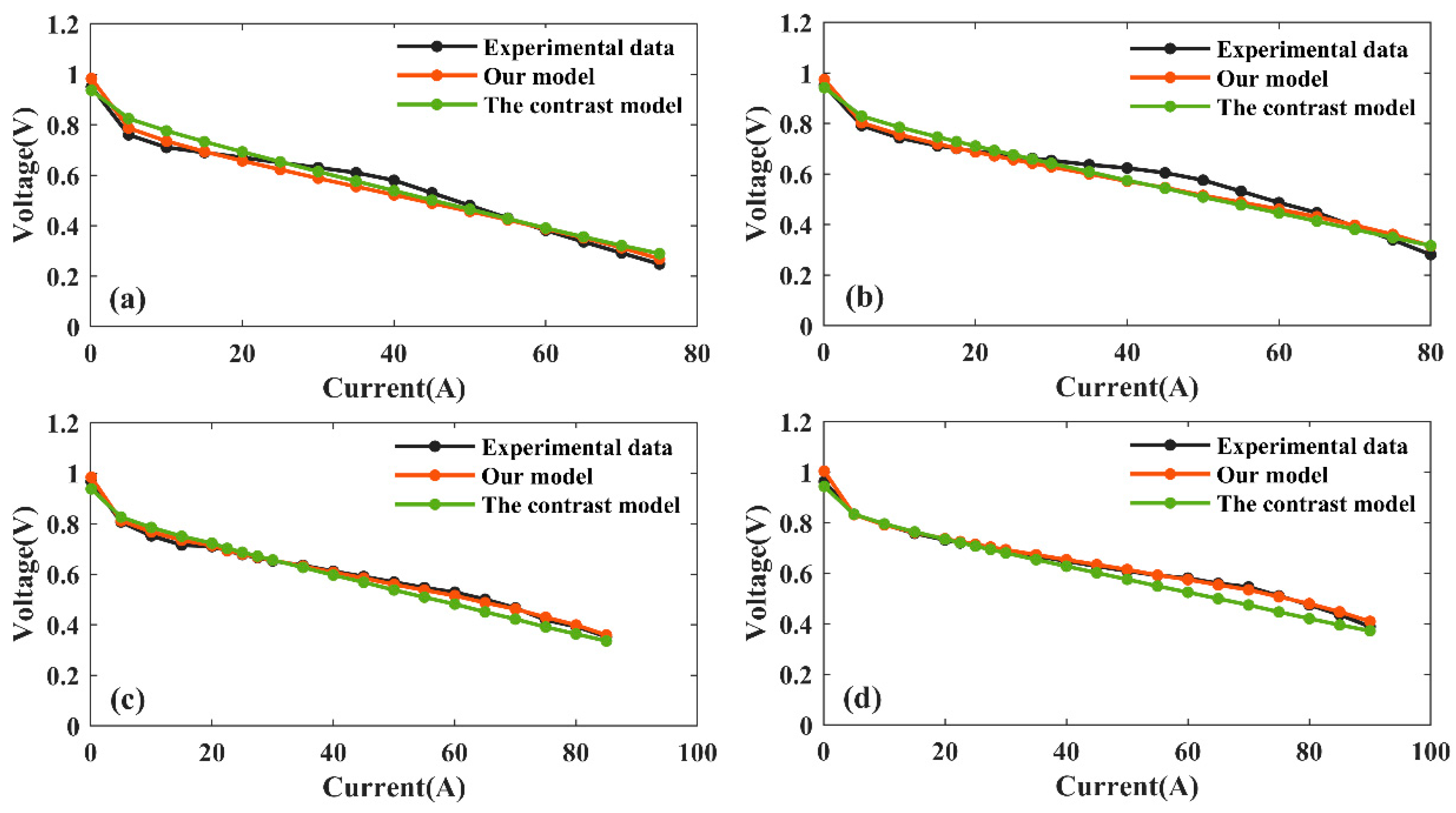
3. Experimental Verification

This study was developed based on the integration of modeling, experimental validation, and analysis techniques. Experiments are designed to verify the correctness and generalization of the model.

3.1. Experimental Platform

As shown in Figure 4a, the platform used in this experiment is the PEMFC test station G60 produced by Greenlight Company. The software EmeraldTM 3.4.3.42 installed on G60 is used to control the operating parameters, measure the current density, and draw the polarization curve. A single PEMFC with an active surface area of $5\times 5 {\mathrm{cm}}^2$ was used for all experiments. The plate adopts a serpentine channel, and the width and height of the channel are 1 mm (Figure 4b). The MEA is manufactured by Gatechn New Energy, with a NafionTM 117 series membrane, 0.2 mg cm⁻² (Pt/Ru) anode catalyst loading, and 0.4 mg cm⁻² (Pt/C) catalyst loading. The GDL is made of carbon fiber cloth, and the porosity is 0.7. The PEM thickness is $15 \mathsf{\mu }\mathrm{m}$.

3.2. Experimental Design and Data Collection

PEMFC performance is mainly affected by temperature, pressure, and humidity. This experiment uses four factors, including fuel cell temperature, anode backpressure, cathode backpressure, and humidity (the same for cathode and anode), as experimental variables. The levels of each factor are determined by selecting some typical values, as shown in

Table 4. Experimental factors and levels.

Factor	Level
	1	2	3
T: Temperature (K)	323	333	343
Pa,out: Anode backpressure (Kpa)	0	20	40
Pc,out: Cathode backpressure (Kpa)	0	20	40
RH: Humidity (%)	30	40	50

. An orthogonal table with four factors and three levels formed is shown in

Table 5. Nine test cases for the experiment.

Test No	Levels				Test No	Levels				Test No	Levels
	T	Pa,out	Pc,out	RH		T	Pa,out	Pc,out	RH		T	Pa,out	Pc,out	RH
1	1	1	1	1	4	2	2	3	1	7	3	3	2	1
2	1	2	2	2	5	2	3	1	2	8	3	1	3	2
3	1	3	3	3	6	2	1	2	3	9	3	2	1	3

.

The experiment is implemented under constant flow mode. The flow rates of the cathode and anode are maintained at 3 L/min and 1.5 L/min, respectively. The PEMFC runs for 2 min after each loading to ensure that a steady state is reached.

3.3. Model Verification

The fixed parameters and fitted parameters representing PEMFC characteristics need to be determined in the model. Fixed parameters are easy to be measured, and their values are given in

Table 6. The fixed parameters.

Parameter	Value	Parameter	Value	Parameter	Value
N	1	${\epsilon }_0$	0.7	$M_{{\mathrm{H}}_2\mathrm{O}}$	18 g/mol
A	25 cm2	d	0.1 cm	$M_{{\mathrm{O}}_2}$	32 g/mol
$L_{\mathrm{mem}}$	0.0015 cm	$L_{\mathrm{MEA}}$	0.0515 cm	$M_{{\mathrm{N}}_2}$	28 g/mol
$L_{\mathrm{GDL}}$	0.025 cm	$N_{\mathrm{ch}}$	29	$M_{{\mathrm{H}}_2}$	2 g/mol
${\rho }_{{\mathrm{H}}_2\mathrm{O}}$	1 g/cm3	$r_{{\mathrm{O}}_2}$	21%	$M_{\mathrm{air}}$	28 g/mol
${\rho }_{\mathrm{mem},\mathrm{dry}}$	1.98 g/cm3	R	8.314 J/mol	$M_{\mathrm{mem},\mathrm{dry}}$	1100 g/mol

. Fitted parameters cannot be reliably measured and need to be estimated by a numerical fitting technique, which have been mentioned in Section 2.2.

In this study, data from six tests were used as training tests to obtain fitted parameters, and data from three tests were retained to validate the semi-empirical model and verify its accuracy. It is worth noting that, to avoid inadequate training, the above six tests were obtained by randomly selecting two tests from test groups 1–3, 4–6, and 7–9, respectively.

According to the above data classification rules, Tests No. 2, 3, 4, 6, 7, and 8 were selected to form a training set for calculating fitted parameters. The remaining Tests No. 1, 5, and 9 formed a validation set to verify the correctness of the model.

To further verify the prediction accuracy of this developed model, the classical semi-empirical model proposed by O’hayre [17], which is widely used in performance prediction [40,41,42] and operation control [43,44,45], was selected as the contrast model. The model can be expressed as follows:

$$V=E_{\mathrm{Nerst}}-V_{\mathrm{act}}-V_{\mathrm{ohm}}-V_{\mathrm{con}}$$

(47)

where $E_{\mathrm{Nerst}}$, $V_{\mathrm{act}}$, and $V_{\mathrm{ohm}}$ are calculated by Equations (35)–(37), respectively. $V_{\mathrm{con}}$ is calculated by the following:

$$V_{\mathrm{con}}=B\ln \left({\displaystyle \frac{i_{\mathrm{L}}}{i_{\mathrm{L}}-i}}\right)$$

(48)

$$i_{\mathrm{L}}=nF{D}_{ij}^{\mathrm{eff}}{\displaystyle \frac{C_{\mathrm{c}}^0}{L_{\mathrm{GDL}}}}$$

(49)

where B is the fitted coefficient and $D_{ij}^{\mathrm{eff}}$ is calculated by Equation (19). Since the contrast model does not consider the dynamic change in GDL porosity, $\epsilon$ is a fixed value of 0.7 in calculation. $C_{\mathrm{c}}^0$ is calculated by Equation (6).

The fitted parameter values and reported values of our model and the contrast model are shown in

Table 7. The fitted parameters.

Parameter	Value in Our Model	Value in Contrast Model	Reported Value
${\alpha }_{\mathrm{c}}$	0.186	0.336	0–2 [46,47]
$i_{0,\mathrm{c}}^{\mathrm{ref}}$	5.3 × 10−8	6.23 × 10−10	5.38 × 10−6 [48], 1 × 10−10 [49]
${\gamma }_{\mathrm{M}}$	42	9	2.7 [50], 111 [51], 446 [52]
$Y_{\mathrm{GDL}}$	0.108	/	0.054 [53]
a	0.0196	/	0.025 [54], 0.044 [24], 0.021 [24]
b	0.23	/	0.144 [55], 0.33 [24], 0.33 [54]
c	0.386	/	−0.207 [55], 0.875 [24], 0.466 [54]
$K_{\mathrm{MEA}}$	6.5 × 10−21	/	1.8 × 10−14 [56], 5 × 10−16 [57]
B	/	0.928	5 × 10−4–1 [58]

. Figure 5a–c show the experimental and predicted data for the validation set.

The comparison of parameters between our study and other research indicates that the charge transfer coefficient (${\alpha }_{\mathrm{c}}$), reference exchange current density ($i_{0,\mathrm{c}}^{\mathrm{ref}}$), roughness factor (${\gamma }_{\mathrm{M}}$), and coefficients b and c are all within the reported value range. Therefore, the calculated values of the above fitted parameters are reasonable. The water amount corresponding to complete flooding ($Y_{\mathrm{GDL}}$) in our study is higher than that in previous studies. However, the GDL porosity is only 0.3 in the report [53], which is lower than the 0.7 porosity in our study, so the fitted parameter $Y_{\mathrm{GDL}}$ is acceptable. Although the fitted parameter a is not within the reported range, it has the same order of magnitude as the reported values. The permeability of the PEM is reported as 1.8 × 10⁻¹⁴ cm² [56] and 5 × 10⁻¹⁶ cm² [57], but the permeability of the MEA in our study is fitted as 6.5 × 10⁻²¹ cm², which is lower than the reported values. However, the GDL on both sides of the PEM can hinder hydraulic permeation, which results in an MEA permeability lower than that of the PEM. Thus, the MEA permeability in our study is reasonable. For the contrast model, the fitted parameters ${\alpha }_{\mathrm{c}}$, $i_{0,\mathrm{c}}^{\mathrm{ref}}$, ${\gamma }_{\mathrm{M}}$, and B are all within the reported value range.

Generalization refers to the ability of the model to describe new data. To verify the generalization ability of our model and the contrast model, a new experiment was designed as a testing set.

Table 8. The level of operating parameters for the testing set.

Parameter	T	${\mathit{P}}_{\mathbf{a},\mathbf{out}}$	${\mathit{P}}_{\mathbf{c},\mathbf{out}}$	RH
Value	353	60	60	60

shows the levels of operating parameters for the testing set, which are outside the range of parameters shown in Table 4. Figure 5d shows the experimental and predicted data for the testing set. The predicted data are obtained by using the real-time operating parameters recorded under experimental conditions in Table 8 as inputs to our model and the contrast model.

Figure 5 shows a comparison between the experimental data and the model prediction data. It is obvious that the error between the model and the experimental data in Figure 5a,b is significantly higher than that in Figure 5c,d. This relatively high model error is primarily attributed to the intrinsic instability of PEMFC operation at a lower temperature. At low temperatures of 50 °C and 60 °C, the proton exchange membrane exhibits insufficient hydration due to a reduced water absorption capacity [59], leading to a non-uniform ionic conductivity. Moreover, air cooling is used to dissipate PEMFC heat in the experiment. Maintaining the PEMFC at low temperatures of 50 °C and 60 °C under a high current density is highly challenging due to increased heat generation. The vigorous heat transfer process causes an uneven temperature distribution within the cell. The semi-empirical model based on a deterministic mass transfer mechanism cannot capture the stochastic voltage fluctuations caused by intrinsic instability.

In this research, root mean squared error (RMSE), mean absolute error (MAE), and maximum absolute error (${\delta }_{\max }$) are used to evaluate the accuracy of the model. The RMSE is calculated as follows:

$$RMSE=\sqrt{{\displaystyle \frac{{\displaystyle {\sum }_{i=1}^n{\left(E_i-{\widehat{E}}_i\right)}^2}}{n}}}$$

(50)

where $E_{\mathrm{i}}$ is the predicted cell voltage using the semi-empirical model, ${\widehat{E}}_i$ is the measured cell voltage from experiment, and n is the number of experimental data.

The MAE is defined by the following:

$$MAE={\displaystyle \frac{1}{n}}{\displaystyle \sum _{i=1}^n{\delta }_i=}{\displaystyle \frac{1}{n}}{\displaystyle \sum _{i=1}^n\left|E_i-{\overline{E}}_i\right|}$$

(51)

where ${\delta }_i$ is the absolute error for the ith data point.

The maximum absolute error is calculated as follows:

$${\delta }_{\max }=\max \left\{{\delta }_1,{\delta }_2,{\delta }_3,\dots ,{\delta }_{\mathrm{n}}\right\}$$

(52)

A comparison of the above three indicators among the validation and testing sets is shown in

Table 9. Indicator calculation of our model and contrast model.

The Set of Experimental Data	Model	$\mathit{n}$	$\mathit{R}\mathit{M}\mathit{S}\mathit{E}\left(\mathbf{V}\right)$	$\mathit{M}\mathit{A}\mathit{E}\left(\mathbf{V}\right)$	${\mathit{\delta }}_{\mathbf{max}}\left(\mathbf{V}\right)$
Validation set	Our model	56	0.025	0.019	0.061
	Contrast model		0.032	0.027	0.067
Testing set	Our model	21	0.012	0.007	0.04
	Contrast model		0.035	0.026	0.071

. In the verification set, the RMSE, MAE, and ${\delta }_{\max }$ of our model are 0.025 V, 0.019 V, and 0.061 V, respectively, which are lower than the indicators of the contrast model. This proves that our model has a better predictive ability than the contrast model. In the testing set, the RMSE, MAE, and ${\delta }_{\max }$ of our model are 0.012 V, 0.007 V, and 0.04 V, respectively, which are also lower than calculated results of the contrast model. This indicates that our model has a better generalization ability than the contrast model. In summary, the generally good fit to the experimental data for the validation and testing sets confirms that the effects of operating parameters are well-modeled in this study.

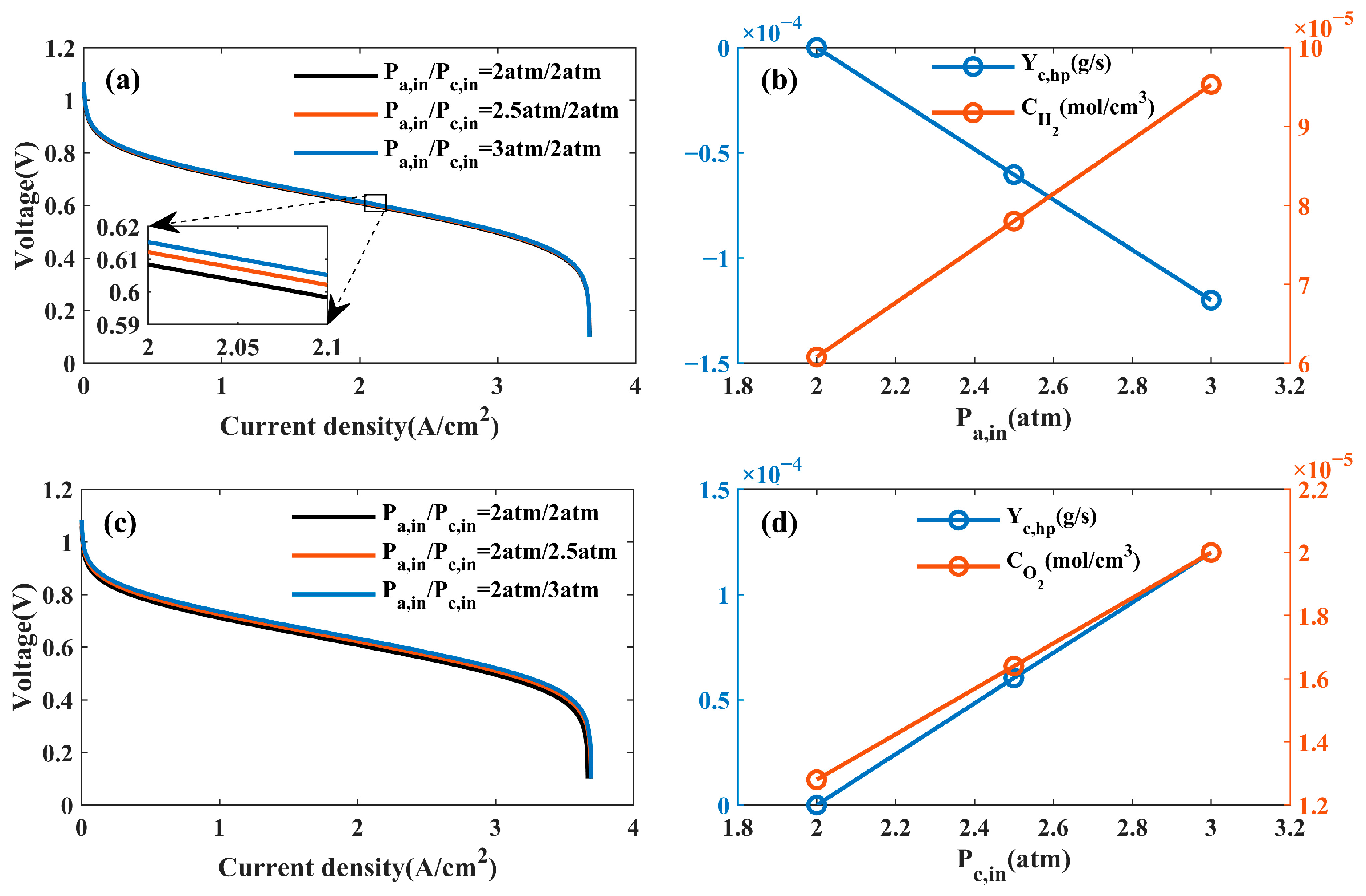
4. Applications of the Semi-Empirical Model

4.1. Analysis of the Effects of Operating Parameters on PEMFC Performance

The semi-empirical model is used to reveal the mechanism behind the effects of temperature and pressure on PEMFC performance. Moreover, the complex influence mechanism of anode and cathode humidity on PEMFC performance is discussed in detail.

4.1.1. Effects of Pressure

The effects of the anode and cathode inlet gas pressure on the PEMFC performance are shown in Figure 6a–c, respectively. As illustrated, an increasing anode and cathode gas pressure can improve PEMFC performance. This is because increasing the gas pressure improves the concentrations of the reactants (as shown at the red lines of Figure 6b–d). The comparison of Figure 6a–c also indicates that, compared with increasing the anode gas pressure, increasing the cathode gas pressure can significantly improve PEMFC performance. This can be attributed to the hydrogen protons passing through the PEM from the anode to the cathode, a reaction that requires the assistance of water molecules diffusing from the cathode side. However, an increase in the anode gas pressure reduces the diffusion of water molecules (as shown at the blue line of Figure 6b), while an increase in cathode pressure enhances the diffusion of water molecules (as shown at the blue line of Figure 6d). As a result, PEMFC performance is significantly improved by increasing the cathode pressure compared with increasing the anode pressure.

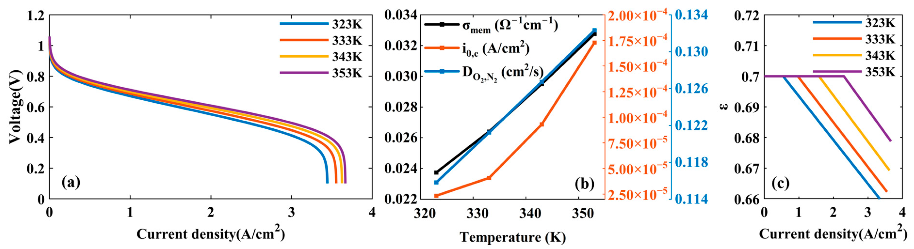
4.1.2. Effects of Temperature

The effects of an operating temperature ranging from 323 K to 353 K on PEMFC performance are shown in Figure 7. PEMFC performance is improved for the whole current density with cell temperature increases from 323 K to 353 K. A relatively high temperature reinforces the catalyst activity and thermal motion of the reactant gas molecules and charge carriers, which, in turn, increase the exchange current density ($i_{0,\mathrm{c}}$), the effective binary diffusion coefficient ($D_{{\mathrm{O}}_2\text{-}{\mathrm{N}}_2}$), and the membrane conductivity (${\sigma }_{\mathrm{mem}}$) (as shown in the Figure 7b). As a result, the chemical reaction is easier to carry out and PEMFC performance improves. Meanwhile, as shown in Figure 7c, the effective porosity increases as the cell temperature increases from 323 K to 353 K, because a high temperature keeps the water as gas and alleviates the cathode flooding.

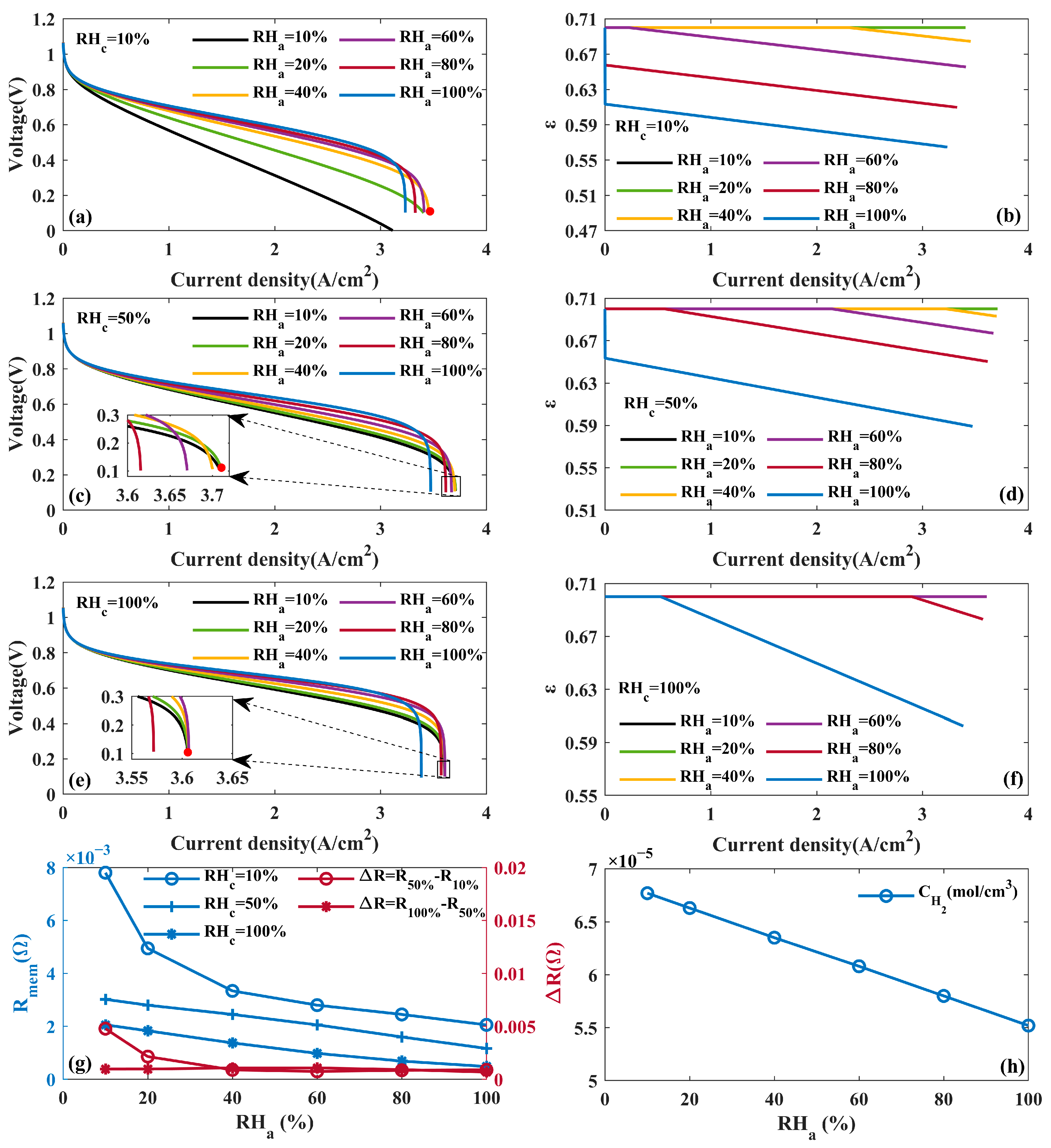
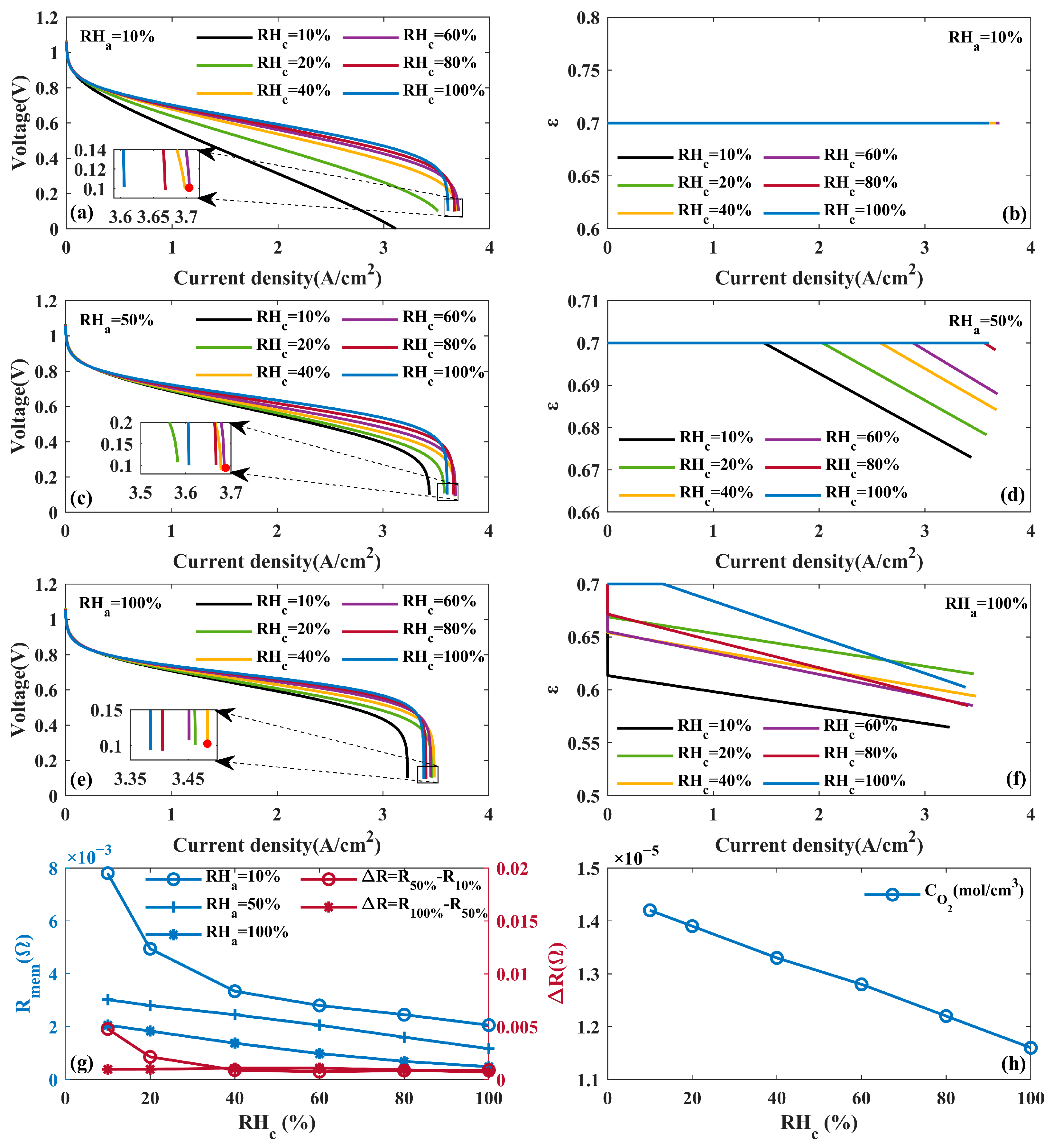
4.1.3. Effects of Humidity

Polarization curves for different reactant humidity levels of the anode and cathode are shown in Figure 8 and Figure 9. At a low current density, increasing the anode or cathode humidity leads to an improvement in the fuel cell performance. The reason for this phenomenon is that a relatively high anode or cathode humidity can improve the water content of the membrane and reduce resistance (as shown at the blue lines of Figure 8g and Figure 9g). It also can be found that, when the air or hydrogen humidity increases from 10% to 50%, PEMFC performance is significantly improved. However, when the reactant is fully humidified (RH_c = 100% or RH_a = 100%), PEMFC performance is not significantly improved compared with the medium humidity level (RH_c = 50% or RH_a = 50%). These results suggest that the membrane has already reached a good hydrating condition under the medium humidity level. Thus, a higher level cannot significantly promote hydration and reduce membrane resistance (as shown at the red lines of Figure 8g and Figure 9g, ${\mathrm{R}}_i$ and $\Delta \mathrm{R}$ in the legend represent the resistance at the corresponding humidity and the resistance changes at two different humidities respectively, and the subscript i is 10%, 50%, or 100%).

At a high current density, as the cathode humidity increases from 10% to 50% and then to 100%, the anode humidity corresponding the maximum limiting current density (red point) changes from 40% to 20% and then to 10% by comparing Figure 8a,c,e. This indicates that the maximum limiting current density can be reached at a lower anode humidity as the cathode humidity increases from 10% to 50% and then to 100%. At a low anode humidity (RH_a = 10% or RH_a = 20%), the GDL porosity remains at 0.7 and the PEM resistance decreases with an increase in cathode humidity, indicating that the maximum limiting current density is obtained due to the PEM resistance decrease rather than the change in GDL porosity. Meanwhile, as shown in Figure 8h, the hydrogen concentration increases as the anode humidity decreases. The comparison of Figure 9a,c,e shows that, as the anode humidity increases from 10% to 50% and then to 100%, the cathode humidity corresponding the maximum limiting current density changes from 60% to 40%. This indicates that the maximum limiting current density can be reached at a lower cathode humidity as the anode humidity increases from 10% to 50% and then to 100%. The relatively high anode humidity increases the water content of the anode and limits back diffusion from the cathode to the anode, which aggravates the cathode flooding. However, the cathode flooding alleviates (as shown at the yellow and purple lines of Figure 9b,d,f) and oxygen concentration increases (as shown in Figure 9h) as the cathode humidity decreases. As a result, cathode mass transport is promoted and the maximum limiting current density is reached at a lower cathode humidity.

4.2. Analysis of the Effects of Structural Parameters on PEMFC Performance

In long-term work, changes in physical parameters such as GDL porosity and PEM thickness will affect PEMFC performance. These parameters are also important physical factors related to PEMFC performance degradation.

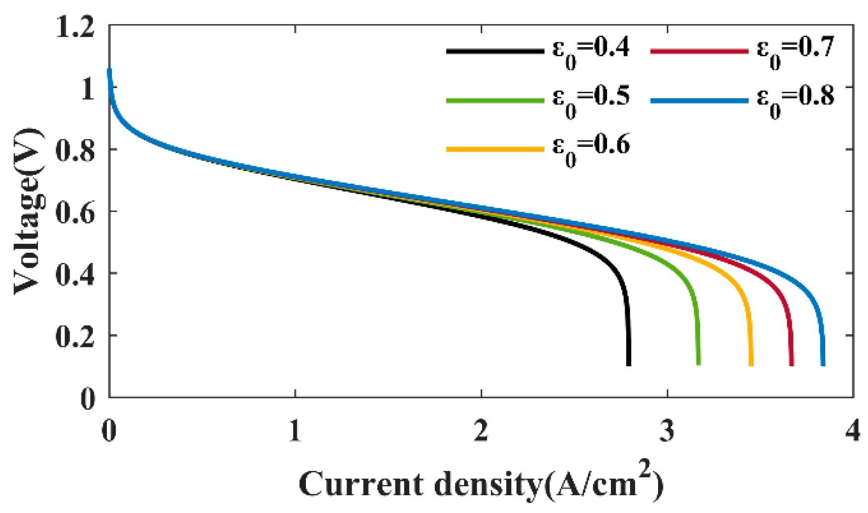
4.2.1. Effects of GDL Porosity

PEMFC performance is influenced by the GDL porosity, and the results are presented in Figure 10. Porosity mainly affects concentration loss, and PEMFC performance improves as GDL porosity increases. A higher porosity reduces cathode flooding at a high current density, which, in turn, improves the gas diffusion and increases the gas concentration on the catalyst surface. As a result, the PEMFC performance is enhanced. However, excessively high GDL porosity will reduce solid support, so material and structural innovations are imperative to develop GDLs exhibiting both high porosity and mechanical robustness.

4.2.2. Effects of PEM Thickness

Polarization curves of different PEM thickness are shown in Figure 11. It is obvious that, as the membrane thickness increases, PEMFC performance decreases at a low current density. This is mainly due to the membrane resistance increasing as the membrane thickness increases (as shown at the green line of Figure 11i), which will cause a more serious ohmic loss. At a high current density, it can be found that the cell performance is strongly related to the gas humidity of the cathode and anode rather than the pressure. When the anode humidity is higher than the cathode humidity, the limiting current density increases with an increase in PEM thickness. The thicker PEM eases water transport from the anode to the cathode by back diffusion, which alleviates the reduction in the cathode GDL effective porosity (as shown at the line of Figure 11b or Figure 11d) and the limitation of oxygen transport. As a result, the limiting current density increases. When the anode humidity is lower than the cathode humidity, it is observed that the limiting current density decreases with an increase in PEM thickness. This opposite result to the case of $R{H}_{\mathrm{a}}>R{H}_{\mathrm{c}}$ is because the thicker PEM obstructs the water transport from the cathode to the anode by back diffusion, which leads to a lower cathode GDL effective porosity (as shown at the line of Figure 11f or Figure 11h) and more serious oxygen transport limitations.

4.3. Optimization of Operating Parameters

A semi-empirical model involving temperature, humidity, and pressure is presented and validated in this study. Meanwhile, the structural parameters of many important components are introduced in the modeling process, including the thickness and porosity of GDL, the active area of the catalyst, and the thickness of the PEM. Therefore, if the degradation law of components with time can be determined, the model can be used to describe the PEMFC output performance in long-term operation. The mathematical model is simply described as follows:

$$V_{\mathrm{cell}}=f\left(T,P_{\mathrm{a},\mathrm{in}},P_{\mathrm{c},\mathrm{in}},P_{\mathrm{a},\mathrm{out}},P_{\mathrm{c},\mathrm{out}},R{H}_{\mathrm{a},\mathrm{in}},R{H}_{\mathrm{c},\mathrm{in}},L_{\mathrm{mem}}\left(t\right),A\left(t\right),{\epsilon }_0\left(t\right),i\right)$$

(53)

The semi-empirical model can accurately capture the effects of operating parameters on PEMFC performance in the whole current density range. Therefore, it can be used to optimize the operating parameters of PEMFC devices steadily working at a high current density. The optimization objective and constraints can be expressed as follows:

$$\begin{array}{l}opt {\displaystyle \frac{V_{\mathrm{cell}}-V_{\mathrm{set}}}{V_{\mathrm{set}}}}\le \omega \\ s. t.\left\{\begin{array}{c}P\in \left(a,b\right)\\ T\in \left(c,d\right)\\ RH\in \left(e,f\right)\end{array}\right.\end{array}$$

(54)

where V_set is the target voltage; $\omega$ is the relative error; P is the gas pressure; T is the temperature; RH is the humidity; a, c, and e are the lower bounds of the parameter range; and b, d, and f are the upper bounds of the parameter range.

4.4. Solution of Physical Coefficients

Five important physical meaningful coefficients are introduced in the process of building the semi-empirical model, including the cathode charge transfer coefficients (${\alpha }_{\mathrm{c}}$), the exchange current density in the reference state ($i_{0,\mathrm{c}}^{\mathrm{ref}}$), the roughness factor (${\gamma }_{\mathrm{M}}$), the water amount corresponding to complete flooding ($Y_{\mathrm{GDL}}$), and the MEA permeability ($K_{\mathrm{MEA}}$). These physical coefficients can be obtained by optimizing the experimental design and solution algorithms. The optimization objective and constraints can be described as follows:

$$\begin{array}{l}opt W_{\mathrm{pre}}-W_{\exp }\le \sigma \\ s. t.\left\{\begin{array}{c}\begin{array}{c}{\alpha }_{\mathrm{c}}\in \left(a,b\right)\\ i_{0,\mathrm{c}}^{\mathrm{ref}}\in (c,d)\end{array}\\ \begin{array}{c}{\gamma }_{\mathrm{M}}\in \left(e,f\right)\\ Y_{\mathrm{GDL}}\in \left(g,h\right)\\ K_{\mathrm{MEA}}\in \left(i,j\right)\end{array}\end{array}\right.\end{array}$$

(55)

where $W_{\mathrm{pre}}$ is the predicted value; $W_{\exp }$ is the experimental value; $\sigma$ is the absolute error; a, c, e, g, and i are the lower bounds of the parameter range; and b, d, f, h, and j are the upper bounds of the parameter range.

5. Conclusions

A semi-empirical model of a PEMFC was developed by reconstructing concentration loss in this study. The effects of the operating parameters, structural parameters, and possible applications of the semi-empirical model were discussed. The characteristics and limitations of this study are summarized as follows:

(1)

Important physical phenomena including reactant transport, water transport, and phase changes are considered in the modeling process to improve the accuracy and interpretability of the semi-empirical model. The model can be used to describe PEMFC polarization with different sizes and flow field structures, because the coefficients $h_{\mathrm{m}}$ and $D_{ij}^{\mathrm{eff}}$, representing the flow field and GDL mass transfer capacity, are quantified in detail.

(2)

An orthogonal experiment was designed with temperature, humidity, anode back pressure, and cathode back pressure as experimental variables. Its higher prediction accuracy and generalization ability than the contrast model indicate that the influence of operating parameters on PEMFC performance is well-modeled in this study.

(3)

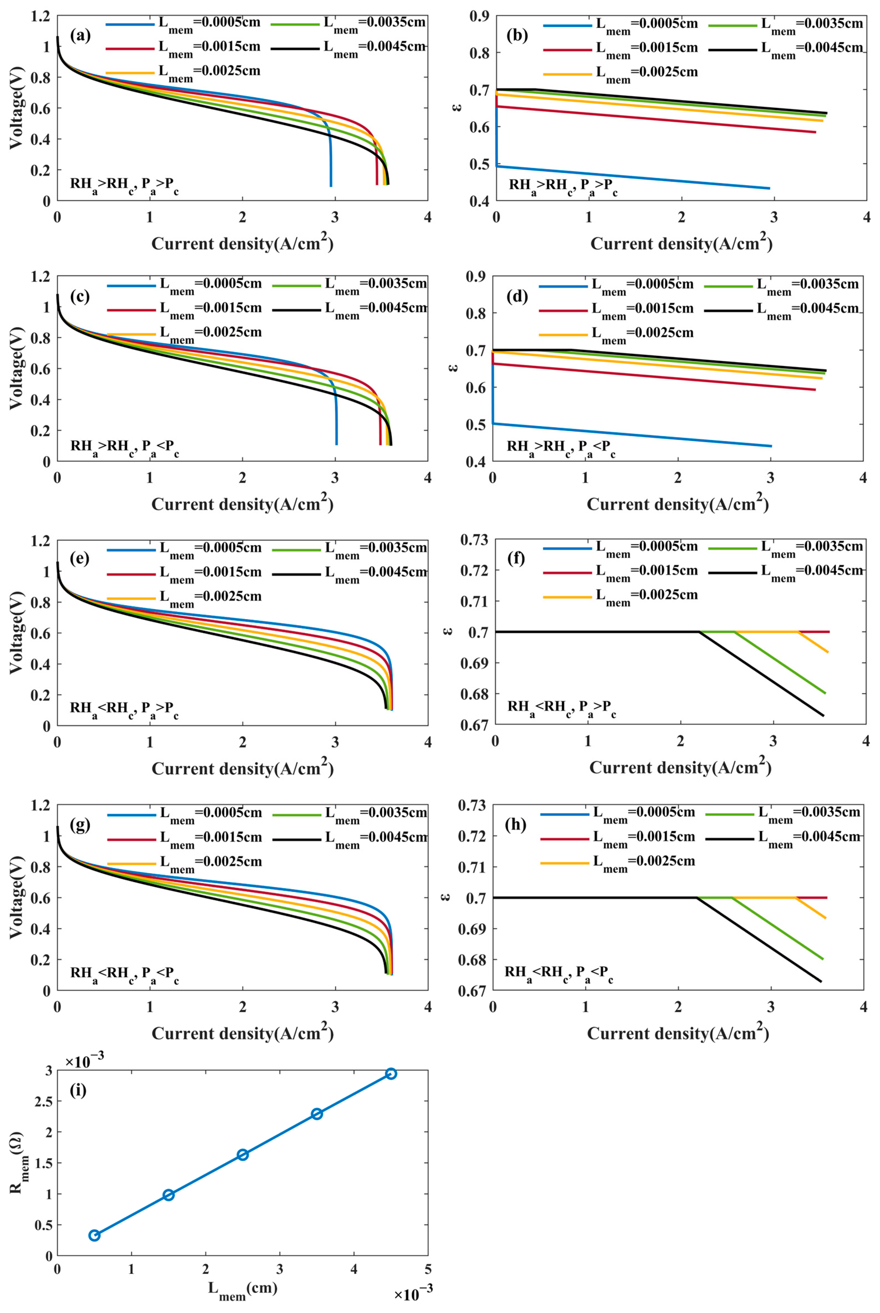
The effects of the operating parameters and physical parameters on PEMFC performance were analyzed. It was found that a relatively high operating temperature, pressure, relative humidity, GDL porosity, and lower PEM thickness can increase PEMFC performance at a low current density. PEMFC performance will decrease if the relative humidity is too high at a high current density. Moreover, the effect of the PEM thickness on PEMFC performance is closely related to the anode and cathode humidity at a high current density. Specifically, PEMFC performance increases with an increasing PEM thickness when $R{H}_{\mathrm{a}}>R{H}_{\mathrm{c}}$, and PEMFC performance decreases with an increasing PEM thickness when $R{H}_{\mathrm{a}}<R{H}_{\mathrm{c}}$.

(4)

The application of the semi-empirical model to predict PEMFC performance considering component degradation in long-term operation was discussed. The optimization of operating parameters for a PEMFC working at a high current density and the solution of important physical coefficients were also prospected.

(5)

The independent impact of “water–gas coupled transport” was isolated in reconstructing concentration loss. This simplification inevitably introduced limitations, such as an inability to describe PEMFC degradation and applicability verification for different flow fields. In the future, we intend to address these limitations by supplementing the degradation model and multiple flow field models on the basis of the current model framework.

References

1. Jung, E.S.; Kim, H.; Kwon, S.; Oh, T.H. Fuel cell system with sodium borohydride hydrogen generator for small unmanned aerial vehicles. Int. J. Green Energy 2018, 15, 385–392. [Google Scholar] [CrossRef]
2. Zhang, G.; Qu, Z.; Wang, N.; Wang, Y. Spatial distribution characteristics in segmented PEM fuel cells: Three-dimensional full-morphology simulation. Electrochim. Acta 2024, 484, 144061. [Google Scholar] [CrossRef]
3. Huo, W.; Fan, L.; Xu, Y.; Benbouzid, M.; Xu, W.; Gao, F.; Li, W.; Shan, N.; Xie, B.; Huang, H. Digitally-assisted structure design of a large-size proton exchange membrane fuel cell. Energy Environ. Sci. 2025, 18, 631–644. [Google Scholar] [CrossRef]
4. Wang, Y.; Diaz, D.F.R.; Chen, K.S.; Wang, Z.; Adroher, X.C. Materials, technological status, and fundamentals of PEM fuel cells–a review. Mater. Today 2020, 32, 178–203. [Google Scholar] [CrossRef]
5. Wang, Y.; Seo, B.; Wang, B.; Zamel, N.; Jiao, K.; Adroher, X.C. Fundamentals, materials, and machine learning of polymer electrolyte membrane fuel cell technology. Energy AI 2020, 1, 100014. [Google Scholar] [CrossRef]
6. Zine, Y.; Benmouna, A.; Becherif, M.; Hissel, D. Towards maximum efficiency of an open-cathode PEM fuel cell system: A comparative experimental demonstration. Int. J. Hydrogen Energy 2024, 86, 72–85. [Google Scholar] [CrossRef]
7. Jiao, K.; Xuan, J.; Du, Q.; Bao, Z.; Xie, B.; Wang, B.; Zhao, Y.; Fan, L.; Wang, H.; Hou, Z. Designing the next generation of proton-exchange membrane fuel cells. Nature 2021, 595, 361–369. [Google Scholar] [CrossRef]
8. Stoll, J.; Zhao, N.; Yuan, X.-Z.; Girard, F.; Kjeang, E.; Shi, Z. Impacts of cathode catalyst layer defects on performance and durability in PEM fuel cells. J. Power Sources 2023, 583, 233565. [Google Scholar] [CrossRef]
9. Dou, S.; Hao, L.; Wang, Q.; Liu, H. Effects of agglomerate structure and operating humidity on the catalyst layer performance of PEM fuel cells. Appl. Energy 2024, 355, 122211. [Google Scholar] [CrossRef]
10. Soltani, M.; Amin, H.M.; Cebe, A.; Ayata, S.; Baltruschat, H. Metal-supported perovskite as an efficient bifunctional electrocatalyst for oxygen reduction and evolution: Substrate effect. J. Electrochem. Soc. 2021, 168, 034504. [Google Scholar] [CrossRef]
11. Zhou, Y.; Chen, B.; Meng, K.; Zhou, H.; Chen, W.; Zhang, N.; Deng, Q.; Yang, G.; Tu, Z. Optimal design of a cathode flow field for performance enhancement of PEM fuel cell. Appl. Energy 2023, 343, 121226. [Google Scholar] [CrossRef]
12. Liu, M.; Fan, W.; Lu, G. Study on mass transfer enhancement of locally improved structures and the application in serpentine and parallel flow fields of PEM fuel cells. Int. J. Hydrogen Energy 2023, 48, 19248–19261. [Google Scholar] [CrossRef]
13. Choi, J.; Park, Y.; Park, J.; Kim, C.; Heo, S.; Kim, S.-D.; Ju, H. Innovative flow field design strategies for performance optimization in polymer electrolyte membrane fuel cells. Appl. Energy 2025, 377, 124551. [Google Scholar] [CrossRef]
14. Wang, Y.; Zhang, P.; Gao, Y.; He, W.; Zhao, Y.; Wang, X. Optimal design of cathode gas diffusion layer with arrayed grooves for performance enhancement of a PEM fuel cell. Renew. Energy 2022, 199, 697–709. [Google Scholar] [CrossRef]
15. Lee, F.; Ismail, M.; Zhang, K.; Ingham, D.; Aldakheel, F.; Hughes, K.; Ma, L.; El-Kharouf, A.; Pourkashanian, M. Optimisation and characterisation of graphene-based microporous layers for polymer electrolyte membrane fuel cells. Int. J. Hydrogen Energy 2024, 51, 1311–1325. [Google Scholar] [CrossRef]
16. Yoon, K.R.; Lee, K.A.; Jo, S.; Yook, S.H.; Lee, K.Y.; Kim, I.D.; Kim, J.Y. Mussel-Inspired Polydopamine-Treated Reinforced Composite Membranes with Self-Supported CeOx Radical Scavengers for Highly Stable PEM Fuel Cells. Adv. Funct. Mater. 2019, 29, 1806929. [Google Scholar] [CrossRef]
17. O’hayre, R.; Cha, S.-W.; Colella, W.; Prinz, F.B. Fuel Cell Fundamentals; John Wiley & Sons: Hoboken, NJ, USA, 2016. [Google Scholar]
18. Abdin, Z.; Webb, C.; Gray, E.M. PEM fuel cell model and simulation in Matlab–Simulink based on physical parameters. Energy 2016, 116, 1131–1144. [Google Scholar] [CrossRef]
19. Hasegawa, S.; Kimata, M.; Ikogi, Y.; Kageyama, M.; Kawase, M.; Kim, S. Modeling of fuel cell stack for high-speed computation and implementation to integrated system model. ECS Trans. 2021, 104, 3. [Google Scholar] [CrossRef]
20. Jang, J.-H.; Yan, W.-M.; Shih, C.-C. Effects of the gas diffusion-layer parameters on cell performance of PEM fuel cells. J. Power Sources 2006, 161, 323–332. [Google Scholar] [CrossRef]
21. Xia, L.; Ni, M.; He, Q.; Xu, Q.; Cheng, C. Optimization of gas diffusion layer in high temperature PEMFC with the focuses on thickness and porosity. Appl. Energy 2021, 300, 117357. [Google Scholar] [CrossRef]
22. Carcadea, E.; Varlam, M.; Ismail, M.; Ingham, D.B.; Marinoiu, A.; Raceanu, M.; Jianu, C.; Patularu, L.; Ion-Ebrasu, D. PEM fuel cell performance improvement through numerical optimization of the parameters of the porous layers. Int. J. Hydrogen Energy 2020, 45, 7968–7980. [Google Scholar] [CrossRef]
23. Spiegel, C. PEM Fuel Cell Modeling and Simulation Using MATLAB; Elsevier: Amsterdam, The Netherlands, 2011. [Google Scholar]
24. Isaacson, M.; Sonin, A.A. Sherwood number and friction factor correlations for electrodialysis systems, with application to process optimization. Ind. Eng. Chem. Process Des. Dev. 1976, 15, 313–321. [Google Scholar]
25. Ding, Y.; Fu, X.; Xu, L.; Li, J.; Ouyang, M.; Wu, H. Scaling analysis of diffusion–reaction process in proton exchange membrane fuel cell with the second Damköhler number. Chem. Eng. J. 2023, 465, 143011. [Google Scholar] [CrossRef]
26. Wang, C.-T.; Chen, Y.-M.; Tang, R.C.O.; Garg, A.; Ong, H.-C.; Yang, Y.-C. Dominated flow parameters applied in a recirculation microbial fuel cell. Process Biochem. 2020, 99, 236–245. [Google Scholar] [CrossRef]
27. Pukrushpan, J.T. Modeling and Control of Fuel Cell Systems and Fuel Processors; University of Michigan: Ann Arbor, MI, USA, 2003. [Google Scholar]
28. Barbir, F. PEM Fuel Cells: Theory and Practice; Academic Press: Waltham, MA, USA, 2005. [Google Scholar] [CrossRef]
29. Wu, H.-W.; Shih, G.-J.; Chen, Y.-B. Effect of operational parameters on transport and performance of a PEM fuel cell with the best protrusive gas diffusion layer arrangement. Appl. Energy 2018, 220, 47–58. [Google Scholar] [CrossRef]
30. Zamel, N.; Li, X. Effective transport properties for polymer electrolyte membrane fuel cells–with a focus on the gas diffusion layer. Prog. Energy Combust. Sci. 2013, 39, 111–146. [Google Scholar] [CrossRef]
31. del Real, A.J.; Arce, A.; Bordons, C. Development and experimental validation of a PEM fuel cell dynamic model. J. Power Sources 2007, 173, 310–324. [Google Scholar] [CrossRef]
32. Deng, H.; Wang, D.; Xie, X.; Zhou, Y.; Yin, Y.; Du, Q.; Jiao, K. Modeling of hydrogen alkaline membrane fuel cell with interfacial effect and water management optimization. Renew. Energy 2016, 91, 166–177. [Google Scholar] [CrossRef]
33. Chen, X.; Xu, J.; Liu, Q.; Chen, Y.; Wang, X.; Li, W.; Ding, Y.; Wan, Z. Active disturbance rejection control strategy applied to cathode humidity control in PEMFC system. Energy Convers. Manag. 2020, 224, 113389. [Google Scholar] [CrossRef]
34. Ziogou, C.; Voutetakis, S.; Papadopoulou, S.; Georgiadis, M.C. Modeling, simulation and experimental validation of a PEM fuel cell system. Comput. Chem. Eng. 2011, 35, 1886–1900. [Google Scholar] [CrossRef]
35. Ferrara, A.; Polverino, P.; Pianese, C. Analytical calculation of electrolyte water content of a Proton Exchange Membrane Fuel Cell for on-board modelling applications. J. Power Sources 2018, 390, 197–207. [Google Scholar] [CrossRef]
36. Ding, Q.; Zhu, K.-Q.; Yang, C.; Chen, X.; Wan, Z.-M.; Wang, X.-D. Performance investigation of proton exchange membrane fuel cells with curved membrane electrode assemblies caused by pressure differences between cathode and anode. Int. J. Hydrogen Energy 2021, 46, 37393–37405. [Google Scholar] [CrossRef]
37. Amphlett, J.C.; Baumert, R.M.; Mann, R.F.; Peppley, B.A.; Roberge, P.R.; Harris, T.J. Performance modeling of the Ballard Mark IV solid polymer electrolyte fuel cell: I. Mechanistic model development. J. Electrochem. Soc. 1995, 142, 1. [Google Scholar] [CrossRef]
38. Springer, T.E.; Zawodzinski, T.; Gottesfeld, S. Polymer electrolyte fuel cell model. J. Electrochem. Soc. 1991, 138, 2334. [Google Scholar] [CrossRef]
39. Nguyen, T.V.; White, R.E. A water and heat management model for proton-exchange-membrane fuel cells. J. Electrochem. Soc. 1993, 140, 2178. [Google Scholar] [CrossRef]
40. Gouda, E.A.; Kotb, M.F.; El-Fergany, A.A. Jellyfish search algorithm for extracting unknown parameters of PEM fuel cell models: Steady-state performance and analysis. Energy 2021, 221, 119836. [Google Scholar] [CrossRef]
41. Ashraf, H.; Elkholy, M.M.; Abdellatif, S.O.; El-Fergany, A.A. Accurate emulation of steady-state and dynamic performances of PEM fuel cells using simplified models. Sci. Rep. 2023, 13, 19532. [Google Scholar] [CrossRef]
42. Chavan, S.L.; Talange, D.B. Modeling and performance evaluation of PEM fuel cell by controlling its input parameters. Energy 2017, 138, 437–445. [Google Scholar] [CrossRef]
43. Ou, K.; Yuan, W.-W.; Choi, M.; Yang, S.; Kim, Y.-B. Performance increase for an open-cathode PEM fuel cell with humidity and temperature control. Int. J. Hydrogen Energy 2017, 42, 29852–29862. [Google Scholar] [CrossRef]
44. Yakut, Y.B. A new control algorithm for increasing efficiency of PEM fuel cells–Based boost converter using PI controller with PSO method. Int. J. Hydrogen Energy 2024, 75, 1–11. [Google Scholar] [CrossRef]
45. Yin, X.; Wang, X.; Wang, L.; Qin, B.; Liu, H.; Jia, L.; Cai, W. Cooperative control of air and fuel feeding for PEM fuel cell with ejector-driven recirculation. Appl. Therm. Eng. 2021, 199, 117590. [Google Scholar] [CrossRef]
46. Newman, J.S. Electrochemical Systems, 4th ed.; John Wiley & Sons: Hoboken, NJ, USA, 1991. [Google Scholar]
47. Zhu, H.; Kee, R.J. A general mathematical model for analyzing the performance of fuel-cell membrane-electrode assemblies. J. Power Sources 2003, 117, 61–74. [Google Scholar] [CrossRef]
48. Kim, J.; Kim, M.; Kang, T.; Sohn, Y.J.; Song, T.; Choi, K.H. Degradation modeling and operational optimization for improving the lifetime of high-temperature PEM (proton exchange membrane) fuel cells. Energy 2014, 66, 41–49. [Google Scholar] [CrossRef]
49. Wang, B.; Wu, K.; Xi, F.; Xuan, J.; Xie, X.; Wang, X.; Jiao, K. Numerical analysis of operating conditions effects on PEMFC with anode recirculation. Energy 2019, 173, 844–856. [Google Scholar] [CrossRef]
50. Parthasarathy, A.; Srinivasan, S.; Appleby, A.J.; Martin, C.R. Electrode kinetics of oxygen reduction at carbon-supported and unsupported platinum microcrystallite/Nafion® interfaces. J. Electroanal. Chem. 1992, 339, 101–121. [Google Scholar] [CrossRef]
51. Watt-Smith, M.J.; Friedrich, J.M.; Rigby, S.P.; Ralph, T.R.; Walsh, F.C. Determination of the electrochemically active surface area of Pt/C PEM fuel cell electrodes using different adsorbates. J. Phys. D Appl. Phys. 2008, 41, 174004. [Google Scholar] [CrossRef]
52. Xie, Z.; Navessin, T.; Shi, K.; Chow, R.; Wang, Q.P.; Song, D.T.; Andreaus, B.; Eikerling, M.; Liu, Z.S.; Holdcroft, S. Functionally graded cathode catalyst layers for polymer electrolyte fuel cells—II. Experimental study of the effect of Nafion distribution. J. Electrochem. Soc. 2005, 152, A1171. [Google Scholar] [CrossRef]
53. Maggio, G.; Recupero, V.; Pino, L. Modeling polymer electrolyte fuel cells: An innovative approach. J. Power Sources 2001, 101, 275–286. [Google Scholar] [CrossRef]
54. El-Genk, M.S.; Toumier, J.M.P. Sherwood number correlation for nuclear graphite gasification at high temperature. Prog. Nucl. Energy 2013, 62, 26–36. [Google Scholar] [CrossRef]
55. Kim, H.; Kim, J.; Kim, D.; Kim, G.H.; Kwon, O.; Cha, H.; Choi, H.; Yoo, H.; Park, T. Mass diffusion characteristics on performance of polymer electrolyte membrane fuel cells with serpentine channels of different width. Int. J. Heat Mass Transf. 2022, 183, 122106. [Google Scholar] [CrossRef]
56. Bernardi, D.M.; Verbrugge, M.W. A Mathematical Model of the Solid-Polymer-Electrolyte Fuel Cell. J. Electrochem. Soc. 1992, 139, 2477. [Google Scholar] [CrossRef]
57. Chen, Q.; Wang, Y.; Yang, F.; Xu, H. Two-dimensional multi-physics modeling of porous transport layer in polymer electrolyte membrane electrolyzer for water splitting. Int. J. Hydrogen Energy 2020, 45, 32984–32994. [Google Scholar] [CrossRef]
58. Zhou, H.; Wu, X.; Li, Y.; Fan, Z.; Chen, W.; Mao, J.; Deng, P.; Wik, T. Model optimization of a high-power commercial PEMFC system via an improved grey wolf optimization method. Fuel 2024, 357, 129589. [Google Scholar] [CrossRef]
59. Majsztrik, P.W.; Satterfield, M.B.; Bocarsly, A.B.; Benziger, J.B. Water sorption, desorption and transport in Nafion membranes. J. Membr. Sci. 2007, 301, 93–106. [Google Scholar] [CrossRef]
Figure 1. Convection and diffusion transport of reactant gas in PEMFC.
Energies 18 01754 g001
Figure 2. Water transport in PEMFC.
Energies 18 01754 g002
Figure 3. The output voltage and voltage loss of fuel cell.
Energies 18 01754 g003
Figure 4. Single fuel cell testing. ((a) G60 test station; (b) Serpentine channel used for test).
Energies 18 01754 g004
Figure 5. The comparison between experimental data and predicted data. ((a) Test No. 1 within validation set; (b) Test No. 5 within validation set; (c) Test No. 9 within validation set; and (d) Testing set).
Energies 18 01754 g005
Figure 6. Effects of pressure on PEMFC performance. ((a) Voltage variation with anode inlet gas pressure; (b) Variation of hydrogen concentration and water molecules diffusion with anode pressure; (c) Voltage variation with cathode inlet gas pressure; (d) Variation of oxygen concentration and water molecules diffusion with cathode pressure. Other operating parameter settings in simulation: P c , out = 1.5   atm ,   R H a , in = R H c , in = 60 % ,   T = 353   K ).
Energies 18 01754 g006
Figure 7. Effects of temperature on PEMFC performance. ((a) Voltage variation with temperature; (b) Variation of membrane conductivity, exchange current density and effective binary diffusion coefficient with temperature; (c) Effective porosity variation with temperature. Other operating parameter settings in simulation: P c , out = 1.5   atm ,   P c , in = P a , in = 2   atm ,   R H a , in = R H c , in = 60 % ).
Energies 18 01754 g007
Figure 8. Effects of anode humidity on PEMFC performance. ((a) Voltage variation with anode humidity under fixed 10%RH cathode humidity; (b) Effective porosity variation with anode humidity under fixed 10%RH cathode humidity; (c) Voltage variation with anode humidity under fixed 50%RH cathode humidity; (d) Effective porosity variation with anode humidity under fixed 50%RH cathode humidity; (e) Voltage variation with anode humidity under fixed 100%RH cathode humidity; (f) Effective porosity variation with anode humidity under fixed 100%RH cathode humidity; (g) Variation of membrane resistance and resistance changes with anode humidity; (h) Variation of hydrogen concentration with anode humidity. Other operating parameter settings in simulation: P c , out = 1.5   atm ,   P c , in = P a , in = 2   atm ,   T = 353   K ).
Energies 18 01754 g008
Figure 9. Effects of cathode humidity on PEMFC performance. ((a) Voltage variation with cathode humidity under fixed 10%RH anode humidity; (b) Effective porosity variation with cathode humidity under fixed 10%RH anode humidity; (c) Voltage variation with cathode humidity under fixed 50%RH anode humidity; (d) Effective porosity variation with cathode humidity under fixed 50%RH anode humidity; (e) Voltage variation with cathode humidity under fixed 100%RH anode humidity; (f) Effective porosity variation with cathode humidity under fixed 100%RH anode humidity; (g) Variation of membrane resistance and resistance changes with cathode humidity; (h) Variation of oxygen concentration with cathode humidity. Other operating parameter settings in simulation: P c , out = 1.5   atm ,   P c , in = P a , in = 2   atm ,   T = 353   K ).
Energies 18 01754 g009
Figure 10. Effects of GDL porosity on PEMFC performance. (Other operating parameter settings: P c , out = 1.5   atm ,   P c , in = P a , in = 2   atm ,   R H a = R H c = 60 % ,   T = 353   K ).
Energies 18 01754 g010
Figure 11. Effects of membrane thickness on PEMFC performance. ((a) Voltage variation with PEM thickness when R H a > R H c and P a > P c ; (b) Effective porosity variation with PEM thickness when R H a > R H c and P a > P c ; (c) Voltage variation with PEM thickness when R H a > R H c and P a < P c ; (d) Effective porosity variation with PEM thickness when R H a > R H c and P a < P c ; (e) Voltage variation with PEM thickness when R H a < R H c and P a > P c ; (f) Effective porosity variation with PEM thickness when R H a < R H c and P a > P c ; (g) Voltage variation with PEM thickness when R H a < R H c and P a < P c ; (h) Effective porosity variation with PEM thickness when R H a < R H c and P a < P c ; (i) Variation of membrane resistance with PEM thickness. Other operating parameter settings in simulation: (a) Pc,out = 1.5 atm, Pa,in = 3 atm, Pc,in = 2 atm, RHa = 100%, RHc = 60%, T = 353 K; (b) Pc,out = 1.5 atm, Pa,in = 2 atm, Pc,in = 3 atm, RHa = 100%, RHc = 60%, T = 353 K; (c) Pc,out = 1.5 atm, Pa,in = 3 atm, Pc,in = 2 atm, RHa = 60%, RHc = 100%, T = 353 K; and (d) Pc,out = 1.5 atm, Pa,in = 2 atm, Pc,in = 3 atm, RHa = 60%, RHc = 100%, T = 353 K).
Energies 18 01754 g011