Nonparametric Probabilistic Prediction of Ultra-Short-Term Wind Power Based on MultiFusion–ChronoNet–AMC

Abstract

Accurate forecasting is crucial for enhancing the flexibility and controllability of power grids. Traditional forecasting methods mainly focus on modeling based on a single data source, which leads to an inability to fully capture the underlying relationships in wind power data. In addition, current models often lack dynamic adaptability to data characteristics, resulting in lower prediction accuracy and reliability under different time periods or weather conditions. To address the aforementioned issues, an ultra-short-term hybrid probabilistic prediction model based on MultiFusion, ChronoNet, and adaptive Monte Carlo (AMC) is proposed in this paper. By combining multi-source data fusion and a multiple-gated structure, the nonlinear characteristics and uncertainties of wind power under various input conditions are effectively captured by this model. Additionally, the AMC method is applied in this paper to provide comprehensive, accurate, and flexible ultra-short-term probabilistic predictions. Ultimately, experiments are conducted on multiple datasets, and the results show that the proposed model not only improves the accuracy of deterministic prediction but also enhances the reliability of probabilistic prediction intervals.

1. Introduction

With the acceleration of global energy transformation, wind power has gained widespread application [1,2]. However, despite the significant environmental benefits of wind power, its variable characteristics threaten the dependability of electrical grids. Therefore, accurately predicting fluctuations in wind power, especially for ultra-short-term forecasts, has become a key research topic to improve the efficiency of grid dispatching [3,4].

Deterministic and probabilistic forecasting are the predominant approaches in wind power prediction. Deterministic prediction models are used for numerical prediction, typically by combining historical data with meteorological models [5,6]. A method for short-term wind power prediction based on causal regularization combined with an extreme learning machine (ELM) was proposed in [7], where the ELM was modeled as a structural causal model, and causal regularization terms were introduced to improve the generalization ability of the model. The convolutional neural network (CNN)–long short-term memory (LSTM)–attention mechanism model was proposed in [8], where supervisory control and data acquisition were used to predict offshore wind turbine power. Time-step parameterization and sensor sensitivity analysis were incorporated to improve offshore wind power forecasting and offer assistance for wind turbine operation and maintenance. A low-carbon economic dispatch strategy was introduced in [9], which utilized a gated recurrent unit (GRU). Subsequently, a thermal–electric integrated demand response model was established to adjust the thermal–electric demand ratio, further lowering carbon emissions and expenses in the system.

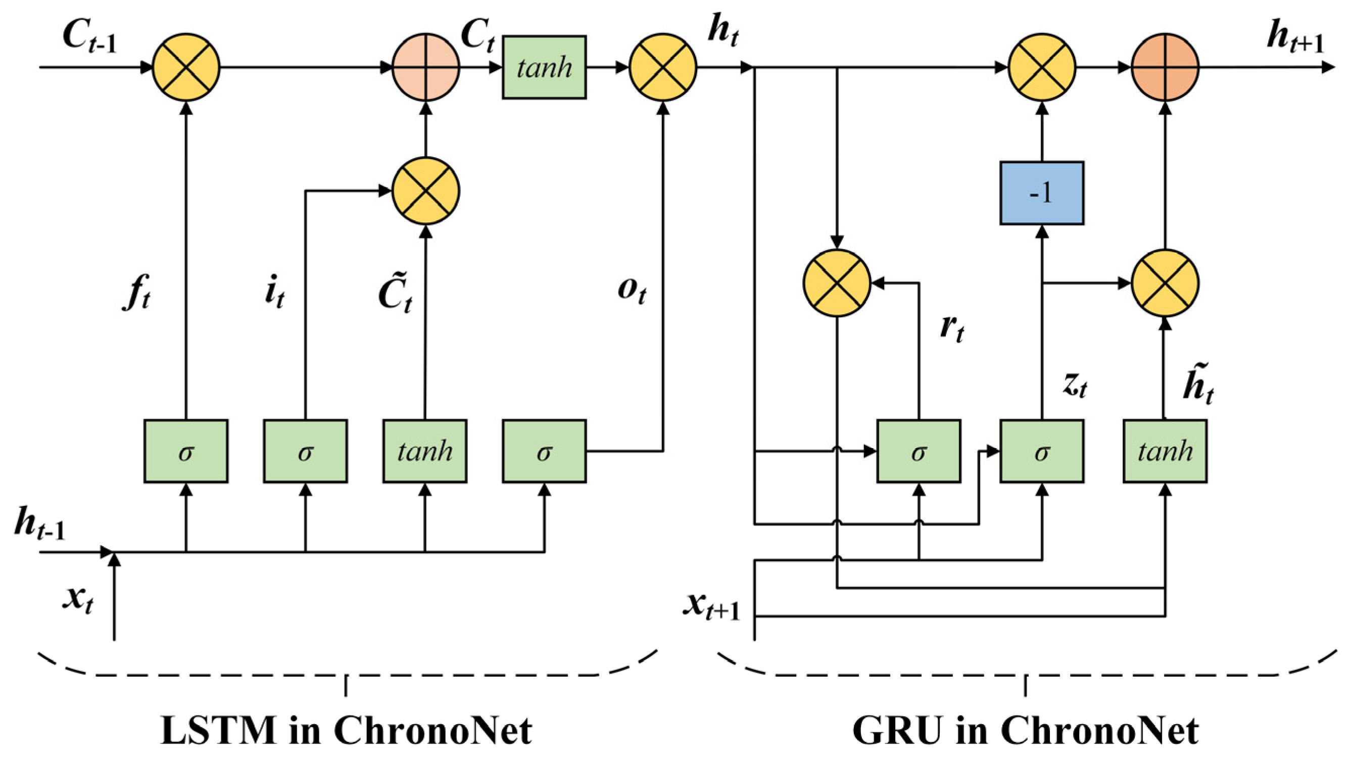
Although existing models have improved prediction accuracy, there are still some limitations in capturing long-term dependencies in certain cases [10]. For example, while LSTM and GRUs are powerful, these methods still face issues like gradient problems and insufficient adaptability when the time steps are very long due to their fixed gating mechanisms [8,9]. The multiple-gated structure and adaptive mechanism were adopted by ChronoNet, which can better capture dynamic dependencies in complex time series and gradually optimize the prediction process based on different features of the data. This not only helps improve model stability but also avoids the modeling difficulties of traditional models on complex data.

Deterministic forecasting methods can provide a single predicted power value, but they fail to accurately reflect the uncertainty of wind power [11]. In contrast, probabilistic forecasting provides a probability distribution, thus offering more comprehensive decision support [12,13]. Modeling error roughness is addressed in [14] by combining historical wind power features, deep belief network feature extraction, and particle swarm optimization algorithms to analyze error time dependence and achieve error correction in ultra-short-term conditional probabilistic wind power prediction models. A multi-output deep neural network was designed in [15], where all quantile estimates were output in a single training process, simplifying the structural complexity of traditional quantile regression (QR) models. The marginal probability density function of a wind farm was generated in [16] using kernel density estimation (KDE), where the KDE bandwidth was optimized, and the golden section search algorithm was employed to reliably predict the power generation for the following day using only three months of historical data. A probabilistic forecasting model was proposed in [17], where the time series was divided into intervals based on error information, and Bootstrap was used to estimate error confidence intervals, overcoming the randomness and instability of seasonal load data by using the interval prediction method.

Among various probabilistic forecasting methods, the Monte Carlo (MC) method can estimate more accurate probabilistic distributions by randomly simulating a large number of samples [18]. A model based on NWP wind speed and MC method was presented in [19], where hierarchical clustering and empirical distribution fitting were used to forecast power fluctuation intervals, and the reliability of the method was verified. It is important to emphasize that the implementation of MC is based on a static model, which means assuming that the relationship between variables is fixed. However, in practical applications, meteorological conditions, environmental factors, and other variables exhibit significant dynamic changes, making the MC method insufficient to adapt to the probability distribution of forecasting errors. To improve efficiency and accuracy, an AMC method is introduced in this paper, which dynamically adjusts the sampling strategy based on the current simulation results to optimize the sample distribution.

Wind power variations are shaped by not just weather conditions, but also by elements like seasonal shifts, terrain, and past power generation data [20]. In reference [21], various environmental factors were integrated, and the features with the highest correlation coefficients were input into the model, validating the effectiveness of the model. The day-ahead joint forecasting method was proposed in [22] by extracting key meteorological factors and integrating deep learning models. However, although existing studies focus on the correlation between wind power features, they typically rely on a single data source, and the analysis methods are inflexible, unable to effectively adapt to the characteristics of different data [23]. Therefore, a Multfusion method, integrating multiple data sources, can overcome the limitations of traditional data.

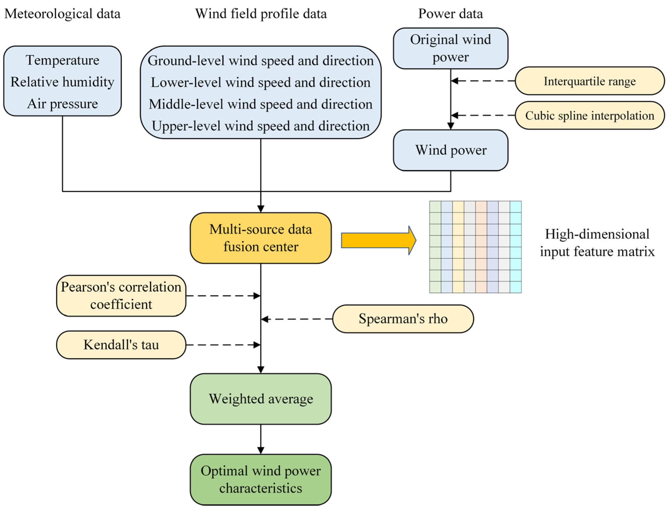
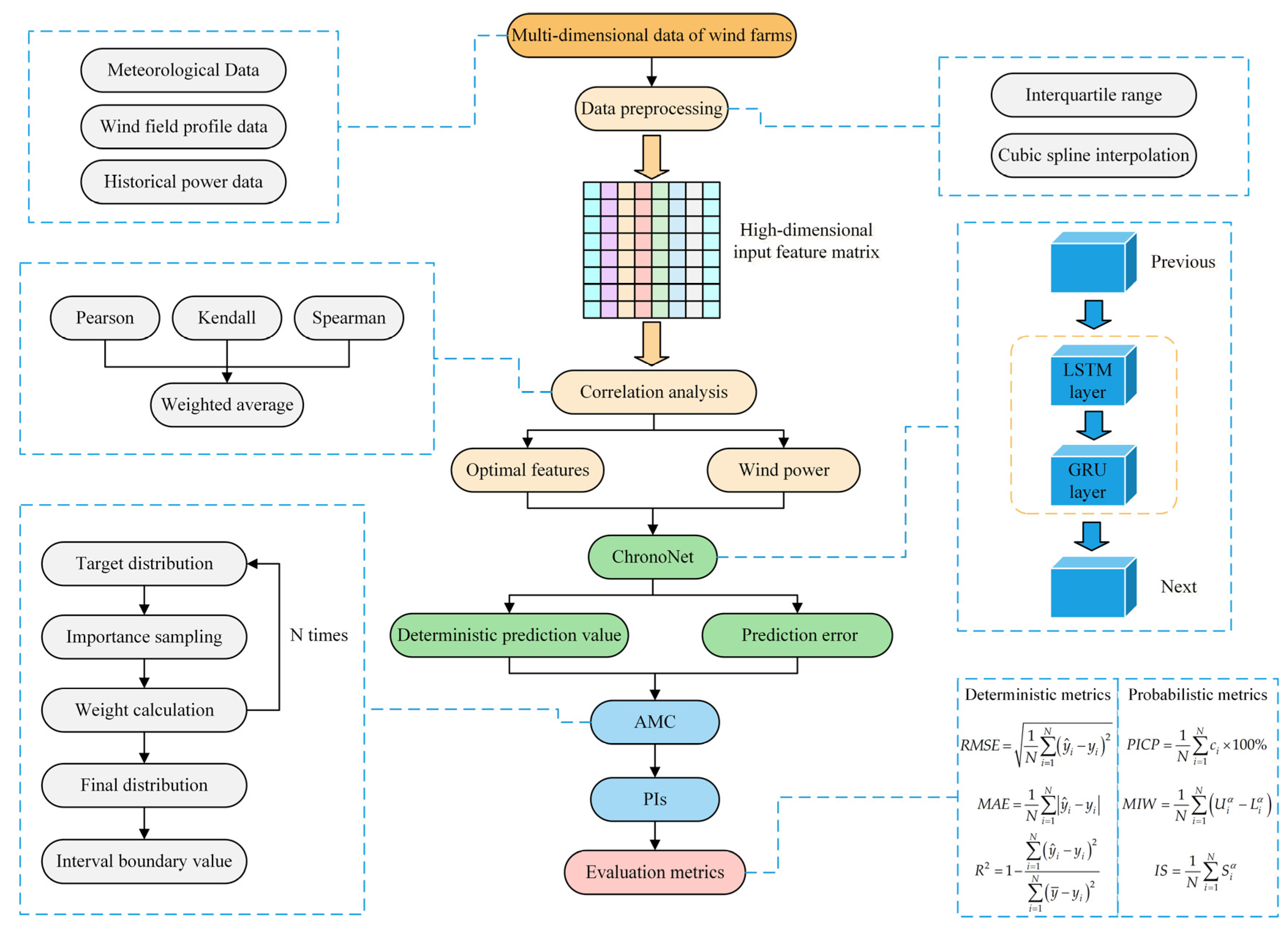
In view of the above issues, a MultiFusion–ChronoNet–AMC-based wind power probabilistic hybrid forecasting model is presented. Firstly, the combination of interquartile range (IQR), cubic spline, and correlation analysis are used to achieve MultiFusion, enhancing the integrity and correlation of the data. Subsequently, through the concatenation of LSTM and GRUs, the ChronoNet multiple-gated network is constructed to obtain deterministic prediction values. Finally, the AMC method is employed to generate adaptive prediction intervals (PIs) under different confidence levels, quantifying the volatility range of wind power. Compared with traditional forecasting models, the main contributions of this paper are as follows:

(1)

MultiFusion is studied to effectively integrate data from different sources through data preprocessing methods and correlation analysis, overcoming issues of data missingness and low-quality data.

(2)

A new model, ChronoNet, is proposed, which balances both long-term and short-term dependencies in time series, enhancing the model’s ability to capture complex time-series data.

(3)

The proposed AMC method can adapt the sampling strategy established on the already sampled data, providing more reliable PIs.

The rest of this paper is organized as follows: Section 2 establishes the theoretical structure; Section 3 introduces the dataset and evaluation metrics; Section 4 analyzes the results; and Section 5 summarizes the paper.

2. Theoretical Structure

2.1. MultiFusion Analysis

As a powerful multi-source fusion method, MultiFusion is composed of IQR, cubic spline, and correlation analysis. Through the integration of these methods, MultiFusion can effectively address issues such as missing data, outliers, and noise in multi-source data, improving data quality and extracting optimal wind power features.

2.1.1. Interquartile Range

IQR is an outlier detection method with strong robustness [24]. It can determine the inner range by calculating the 25th and 75th percentiles of the dataset to remove outlier data. The specific steps of IQR are as follows:

(1)

The elements of the original wind power series P are sorted to obtain an ordered power series $P^{\ast }=\left(p_1,p_2,\dots ,p_n\right),p_1\le p_2\le \dots \le p_n$

(2)

The quartiles $Q_1$, $Q_2$, and $Q_3$ are determined, with the calculation formulas shown in Equations (1)–(3):

$$Q_1=median\left(p_1,p_2,\dots ,p_{⌊{\displaystyle \frac{n}{2}}⌋}\right)$$

(1)

$$Q_2=median\left(p_1,p_2,\dots ,p_n\right)$$

(2)

$$Q_3=median\left(p_{⌊{\displaystyle \frac{n}{2}}⌋+1},p_{⌊{\displaystyle \frac{n}{2}}⌋+2},\dots ,p_n\right)$$

(3)

where median represents the median function and ⌊⌋ represents calculating the largest integer smaller than itself.

(3)

Calculate the inner limit range using Equations (4) and (5):

$$L=Q_1-1.5\left(Q_3-Q_1\right)$$

(4)

$$U=Q_3+1.5\left(Q_3-Q_1\right)$$

(5)

where L and U are the lower and upper limits, respectively. Power values below L or above U are removed.

2.1.2. Cubic Spline

Cubic spline is an interpolation method, where the core idea is to use multiple cubic polynomial segments to fit the missing power values between adjacent data points, thereby avoiding large fluctuations in power data caused by sparse data points [25].

Let there be n + 1 sampling points in the interval $\left[a,b\right]$, with $x_0,x_1,\dots ,x_n$, such that $a=x_0<x_1<x_2<\dots <x_n=b$. The function $f\left(x\right)$ needs to meet the following conditions:

(1)

Interpolation condition: $f\left(x\right)=y_i$, $i=0,1,2,\dots ,n$.

(2)

Second-order derivative continuity: $f^{″}\left(x\right)$ is continuous on the interval $\left[a,b\right]$, i.e., $f\left(x\right)$ has continuous second-order derivatives.

(3)

On each subinterval $\left[x_i,x_{i+1}\right]$, $f\left(x\right)$ is a cubic polynomial.

If the above conditions are satisfied, then the cubic spline function $f_i\left(x\right)$ at the point $x_i$ is given by Equation (6):

$$f_i\left(x\right)=a_i{\left(x-x_i\right)}^3+b_i{\left(x-x_i\right)}^2+c_i\left(x-x_i\right)+d_i,x\in \left[x_i,x_{i+1}\right]$$

(6)

where $a_i$, $b_i$, $c_i$, and $d_i$ are the coefficients of the polynomial function.

2.1.3. Correlation Analysis

Wind power forecasting depends not only on wind speed data but also on meteorological conditions and wind speed profile data [26]. In this paper, multiple correlation coefficients are used to comprehensively assess the linear, nonlinear, and ordinal correlations between multi-source data. By integrating data from multiple source scenarios, the correlation among various features is analyzed to comprehensively capture the dynamic characteristics of the wind power system. The specific approach is illustrated in Figure 1.

The specific steps are as follows:

(1)

Historical meteorological data, wind field profile data at different heights, and power data are collected, with power data being denoised by IQR and completed by cubic spline.

(2)

In the MultiFusion center, a high-dimensional input feature matrix is constructed.

(3)

Correlation coefficients for different types are calculated, with the formulas as shown in Equations (7)–(9).

$$r={\displaystyle \frac{{\displaystyle \sum _{i=1}^n\left(x_i-\overline{x}\right)\left(y_i-\overline{y}\right)}}{\sqrt{{\displaystyle \sum _{i=1}^n{\left(x_i-\overline{x}\right)}^2{\displaystyle \sum _{i=1}^n{\left(y_i-\overline{y}\right)}^2}}}}}$$

(7)

$$\tau ={\displaystyle \frac{2\left(n_c-n_d\right)}{n\left(n-1\right)}}$$

(8)

$$\rho =1-{\displaystyle \frac{6{\displaystyle \sum _{i=1}^n{d}_i^2}}{n\left(n^2-1\right)}}$$

(9)

where $r$ represents the Pearson’s correlation coefficient; $\tau$ represents the Kendall’s tau; $\rho$ represents Spearman’s rho; n is the sample size; $x_i$ and $y_i$ are data points of two variables; $\overline{x}$ and $\overline{y}$ are the means of variables x and y; $n_c$ represents the number of concordant pairs between the data points $\left(x_i,y_i\right)$ and $\left(x_j,y_j\right)$, i.e., $\left(x_i<x_{j}and{y}_i<y_j\right)$ or $\left(x_i>x_{j}and{y}_i>y_j\right)$; $n_d$ represents the number of discordant pairs between the data points $\left(x_i,y_i\right)$ and $\left(x_j,y_j\right)$, i.e., $\left(x_i<x_{j}and{y}_i>y_j\right)$ or $\left(x_i>x_{j}and{y}_i<y_j\right)$; $d_i=R\left(x_i\right)-R\left(y_i\right)$ represents the rank difference in each data pair for variables x and y; and $R\left(x_i\right)$ and $R\left(y_i\right)$ represent the ranks of data points $x_i$ and $y_i$ within their respective variables.

(4)

The fusion correlation coefficient is calculated by weighted average according to Equation (10), and the optimal wind power characteristics are selected.

$$\widehat{r}={\omega }_P\cdot r+{\omega }_K\cdot \tau +{\omega }_S\cdot \rho$$

(10)

where $\widehat{r}$ represents the fusion correlation coefficient; ${\omega }_P$, ${\omega }_K$, and ${\omega }_S$ are the weights of each correlation coefficient, satisfying ${\omega }_P+{\omega }_K+{\omega }_S=1$.

2.2. ChronoNet Model

Traditional recurrent neural networks face the gradient problem when processing long-sequence data, leading to difficulties in training and a decline in model performance [27]. The advent of LSTM and GRUs has achieved some success in mitigating this issue, but they still have certain limitations [28,29]. The limitations of LSTM lie in its computational complexity, slow training, and the potential redundancy caused by its three-gate design. Although the GRU is computationally more efficient, its simpler structure may fail to capture long-term dependencies.

To solve the above problems, ChronoNet retains LSTM’s ability to model long-term dependencies while improving the GRU’s computational efficiency, enhancing the flexibility of the model and improving its ability to process both long and short sequence data. The computational principle of LSTM in ChronoNet is as follows:

In the forget gate $f_t$, ChronoNet selectively forgets information that is irrelevant to the current task. The calculation formula is as shown in Equation (11):

$$f_t=\sigma \left(W_f\cdot \left[h_{t-1},x_t\right]+b_f\right)$$

(11)

where $\sigma$ is the activation function; $W_f$ is the weight; $h_{t-1}$ is the external state; $x_t$ is the input vector; and $b_f$ is the bias term.

In the input gate $i_t$, ChronoNet computes the candidate values ${\tilde{C}}_t$ and then derives the cell state value $C_t$ at time t, as shown in Equations (12)–(14):

$$i_t=\sigma \left(W_i\cdot \left[h_{t-1},x_t\right]+b_i\right)$$

(12)

$${\tilde{C}}_t=\tanh \left(W_C\cdot \left[h_{t-1},x_t\right]+b_C\right)$$

(13)

$$C_t=f_t\cdot C_{t-1}+i_t\cdot {\tilde{C}}_t$$

(14)

where $C_{t-1}$ is the cell state value at time t − 1; $W_i$ and $W_C$ are the weights; $b_i$ and $b_C$ are the bias terms; and tanh is the hyperbolic tangent function.

In the output gate $o_t$, the output is computed using the following formulas Equations (15) and (16):

$$o_t=\sigma \left(W_o\cdot \left[h_{t-1},x_t\right]+b_o\right)$$

(15)

$$h_t=o_t\cdot \tanh \left(C_t\right)$$

(16)

where $h_t$ is the interim hidden state of ChronoNet; $W_o$ is the weight; and $b_o$ is the bias term.

At this point, the LSTM computation is complete, and the GRU section begins. The computation principle of the GRU in ChronoNet is as follows:

In the reset gate $r_t$, ChronoNet controls the influence of the interim hidden state $h_t$ and the new input $x_{t+1}$ on the candidate state. The calculation formula is shown as Equation (17):

$$r_t=\sigma \left(W_r\cdot \left[h_t,x_{t+1}\right]+b_r\right)$$

(17)

where $W_r$ is the weight and $b_r$ is the bias term.

In the update gate $z_t$, ChronoNet controls the weight between the hidden state $h_t$ and the candidate state ${\tilde{h}}_t$, determining how much of the previous information to retain. The calculation formula is as shown in Equation (18):

$$z_t=\sigma \left(W_z\cdot \left[h_t,x_{t+1}\right]+b_z\right)$$

(18)

where $W_z$ is the weight and $b_z$ is the bias term.

ChronoNet combines gate information to update the final hidden state, as shown in Equations (19) and (20):

$${\tilde{h}}_t=\tanh \left[W_h\cdot \left[r_t\cdot h_{t-1},x_t\right]+b_h\right]$$

(19)

$$h_{t+1}=\left(1-z_t\right)\cdot h_t+z_t\cdot {\tilde{h}}_t$$

(20)

where $W_h$ is the weight; $b_h$ is the bias term; and $h_{t+1}$ is the final hidden state of ChronoNet. The structure of ChronoNet is shown in Figure 2.

2.3. Adaptive Monte Carlo

MC is an outstanding random sampling technique in which a large number of computer-generated pseudorandom numbers are utilized to obtain the approximate solution to the problem [30]. However, in most scenarios, different regions have different levels of importance. If the sample size is set too small, MC may sample a significant number of irrelevant regions, leading to inaccurate results [31]. Conversely, if the sample size is set too large, the efficiency of sampling may become lower.

To enable MC to dynamically adjust its sampling strategy and update error distribution parameters in real time, the AMC method is proposed in this paper. AMC is an improved version of MC, in which the importance sampling technique is used to optimize the sample generation process, focusing on generating adaptive PIs in high-probability error regions. The principle is to assume that the current distribution $q\left(\epsilon \right)$ is an importance sampling distribution, and the goal is to adaptively adjust $q\left(\epsilon \right)$ to better approximate the target distribution $p\left(\epsilon \right)$.

The calculation process is as follows:

(1)

Assume the predictive value is $\widehat{P}$, and the forecast error $\epsilon$ follows a known distribution. According to the Central Limit Theorem, when errors from multiple independent factors are combined, their sum tends toward a normal distribution [32]. This means that $\epsilon$ also follows a normal distribution, as shown in Equation (21):

$$\epsilon \sim N\left(\mu ,{\delta }^2\right)$$

(21)

where $\mu$ is the mean of the forecast error and $\delta$ is the standard deviation of the forecast error.

(2)

Generate sample ${\epsilon }_i$ from current importance distribution $q\left({\epsilon }_i\right)$, and then use the probability density function of target distribution $p\left({\epsilon }_i\right)$ for weighted correction. The formula for calculating sample weights $w\left({\epsilon }_i\right)$ is shown in Equation (22):

$$w\left({\epsilon }_i\right)={\displaystyle \frac{p\left({\epsilon }_i\right)}{q\left({\epsilon }_i\right)}}$$

(22)

(3)

The weighted corrected sample can be represented as $\left\{{\epsilon }_i,w\left({\epsilon }_i\right)\right\}$, and based on the corrected sample, the statistical measure ${\widehat{E}}_i$ of the target distribution is calculated by Equation (23):

$${\widehat{E}}_i={\displaystyle \frac{{\displaystyle \sum _{i=1}^n{\epsilon }_i\cdot w\left({\epsilon }_i\right)}}{{\displaystyle \sum _{i=1}^{n}w\left({\epsilon }_i\right)}}}$$

(23)

where n represents the sample size of AMC.

(4)

Building upon the weighted adjustment discussed above, the forecast power limits for each sample is denoted as $P_i$. The formula for these limits is as follows in Equation (24):

$$P_i=\widehat{P}+{\widehat{E}}_i$$

(24)

(5)

Repeat the above step N times to obtain a set of simulated wind power boundary values $P_1,P_2,\dots ,P_N$.

(6)

The PIs are constructed based on the simulation results. Assume a confidence level of $\left(1-\alpha \right)\times 100\%$, then the limits of the PIs correspond to the (1 − α/2)-th and α/2-th percentiles of the simulated results, as shown in Equations (25) and (26):

$$L_P=P_{\left(\alpha /2\times N\right)}$$

(25)

$$U_P=P_{\left(1-\alpha /2\right)\times N}$$

(26)

where $L_P$ represents the lower limit of the PIs and $U_P$ represents the upper limit of the PIs.

2.4. The Proposed Hybrid Forecasting Model

The proposed model is shown in Figure 3. Firstly, multi-dimensional data of wind farms is imported, and a high-dimensional input feature matrix is constructed. Subsequently, the weighted correlation coefficient is calculated, and the optimal features are selected. Thereafter, ChronoNet is trained, and deterministic prediction values are output. Ultimately, the wind power PIs are determined by AMC, combining the deterministic prediction values and prediction errors.

3. Materials and Metrics

3.1. Description of Dataset

The dataset used in this paper comes from a wind farm in China with an installed capacity of 75 megawatts, covering a period of one year. Since spring and autumn seasons have relatively lower energy demand, the power forecast data from winter and summer seasons are selected as they better reflect the model’s performance. The wind farm dataset includes meteorological information, wind field profile data, and historical power data. Each data point has a sampling resolution of 15 min, with 96 samples per day. The dataset is divided into 90% training and 10% testing sets.

During the model training process, the loss function used is MSE. The calculation formula is shown in Equation (27):

$$MSE={\displaystyle \frac{1}{N}}{\displaystyle \sum _{i=1}^N{\left({\widehat{y}}_i-y_i\right)}^2}$$

(27)

where N, ${\widehat{y}}_i$, and $y_i$ represent the sample size, predicted values, and actual values, respectively.

The experiment was conducted on a workstation equipped with Intel (R) Core (TM) i5-9300H CPU @ 2.40 GHz and 8 GB memory, and the programming environment was Matlab 2024b.

3.2. Evaluation Metrics

For deterministic prediction, the root mean square error (RMSE), mean absolute error (MAE), and coefficient of determination (R²) are used as evaluation metrics [33]. The calculation formulas are given by Equations (28)–(30):

$$RMSE=\sqrt{{\displaystyle \frac{1}{N}}{\displaystyle \sum _{i=1}^N{\left({\widehat{y}}_i-y_i\right)}^2}}$$

(28)

$$MAE={\displaystyle \frac{1}{N}}{\displaystyle \sum _{i=1}^N\left|{\widehat{y}}_i-y_i\right|}$$

(29)

$$R^2=1-{\displaystyle \frac{{\displaystyle \sum _{i=1}^N{\left({\widehat{y}}_i-y_i\right)}^2}}{{\displaystyle \sum _{i=1}^N{\left(\overline{y}-y_i\right)}^2}}}$$

(30)

where N, ${\widehat{y}}_i$, $y_i$, and $\overline{y}$ represent the sample size, predicted values, actual values, and the mean of the actual values, respectively.

For probabilistic prediction, the coverage probability of the PIs (PICP), mean interval width (MIW), and interval score (IS) are used as evaluation metrics [34]. The IS represents the overall interval score of the nominal confidence of the PIs (PINC), which integrates both reliability and sharpness, with a value closer to zero indicating better prediction performance. The calculation formulas are given by Equations (31)–(36):

$$PICP={\displaystyle \frac{1}{N}}{\displaystyle \sum _{i=1}^N{c}_i}\times 100\%$$

(31)

$$MIW={\displaystyle \frac{1}{N}}{\displaystyle \sum _{i=1}^N\left(U_i^{\alpha }-L_i^{\alpha }\right)}$$

(32)

$$IS={\displaystyle \frac{1}{N}}{\displaystyle \sum _{i=1}^N{S}_i^{\alpha }}$$

(33)

$$c_i=\left\{\begin{array}{c}1,y_i\in \left[L_i^{\alpha },U_i^{\alpha }\right]\\ 0,y_i\notin \left[L_i^{\alpha },U_i^{\alpha }\right]\end{array}\right.$$

(34)

$$S_i^{\alpha }=\left\{\begin{array}{c}-2\alpha {\zeta }_i^{\alpha }-4\left(L_i^{\alpha }-y_i\right),y_i<L_i^{\alpha }\\ -2\alpha {\zeta }_i^{\alpha },y_i\in \left[L_i^{\alpha },U_i^{\alpha }\right]\\ -2\alpha {\zeta }_i^{\alpha }-4\left(y_i-U_i^{\alpha }\right),y_i>U_i^{\alpha }\end{array}\right.$$

(35)

$${\zeta }_i^{\alpha }=U_i^{\alpha }-L_i^{\alpha }$$

(36)

where $U_i^{\alpha }$ and $L_i^{\alpha }$ represent the upper and lower limits of the PIs, respectively; $c_i$ is an indicator function; $S_i^{\alpha }$ is the score of sample PIs; ${\zeta }_i^{\alpha }$ is the width of sample PIs; and α is the significance level.

4. Case Studies

4.1. Multi-Source Data Fusion Results

The reason why the deterministic prediction model achieves good predictive performance is that it integrates MultiFusion method. The utilization of model resources is optimized by MultiFusion, enabling the model to capture the complex nonlinear and spatiotemporal relationships in the data. Therefore, it is necessary to conduct an analysis of multi-source data fusion.

The results of summer wind power processing are shown in Figure 4. As can be seen, the cleaned power curve not only fills in the missing data but also smooths the data, effectively eliminating unreasonable fluctuations caused by data noise or faults, while maintaining the continuity and physical plausibility of the data.

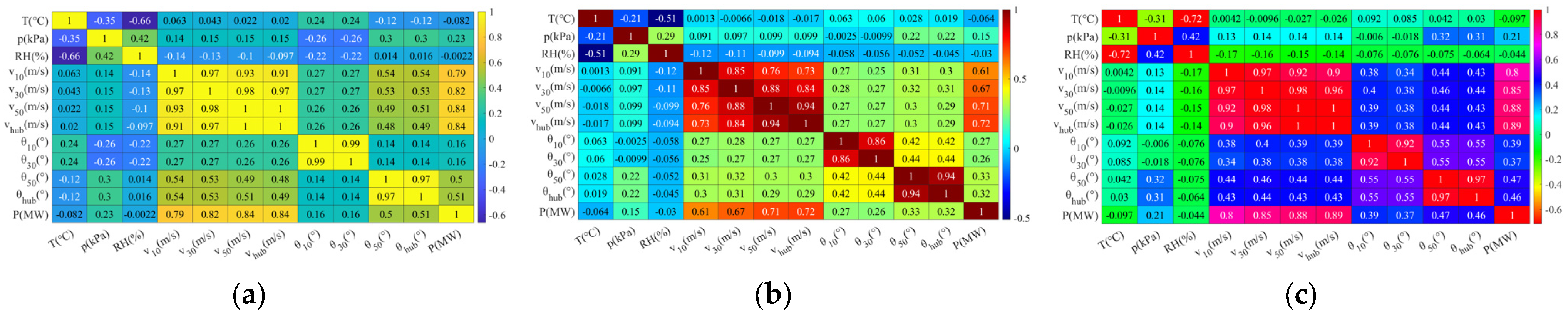
To identify the most relevant features for wind power, a correlation analysis of various features of the wind farm is performed. Pearson, Kendall, and Spearman correlation coefficients are used to study the relationships between different features of the wind farm, and the analysis results are shown in Figure 5. It is clearly observed that meteorological and wind direction data have a weaker correlation with power, while wind speed data shows a stronger correlation with power.

Table 1. Wind power characteristic variables.

Symbol	T	p	RH	v	$\theta$	P
Name	temperature	atmospheric pressure	relative humidity	wind speed	wind direction	wind power

lists the variable names corresponding to various symbols.

To investigate the correlation of wind speed at different profiles,

Table 2. Vertical wind profile correlation.

Vertical Wind Profile	Pearson’s Coefficient	Kendall’s Tau	Spearman’s Rho	Average
Ground level	0.79	0.61	0.80	0.73
Lower level	0.82	0.67	0.85	0.78
Middle level	0.84	0.71	0.88	0.81
Upper level	0.84	0.72	0.89	0.82

provides detailed numerical values. From the “Average” column, it can be observed that the wind speed correlation follows this order: Upper level > Middle level > Lower level > Ground level. Therefore, the Upper-level wind speed is selected as the optimal wind power feature.

4.2. Deterministic Forecasting Analysis

This study selects a series of representative benchmark models, including ELM, CNN, LSTM, GRU, BiLSTM, etc., for comparison with the proposed model. The prediction time scale is ultra-short-term, and the parameter configurations for different models are shown in

Table 3. Model parameters.

Model	ELM	CNN	LSTM	BiLSTM	GRU	ChronoNet
Optimizer	-	Sgdm	Adam	Adam	Adam	Adam
Batch size	-	64	64	64	64	64
Hidden Layers	1	2	2	2	2	2
Hidden units	128	64	64	64	64	64
Max iterations	-	100	100	100	100	100
Learning rate	-	0.005	0.005	0.005	0.005	0.005
Regularization	0.001

.

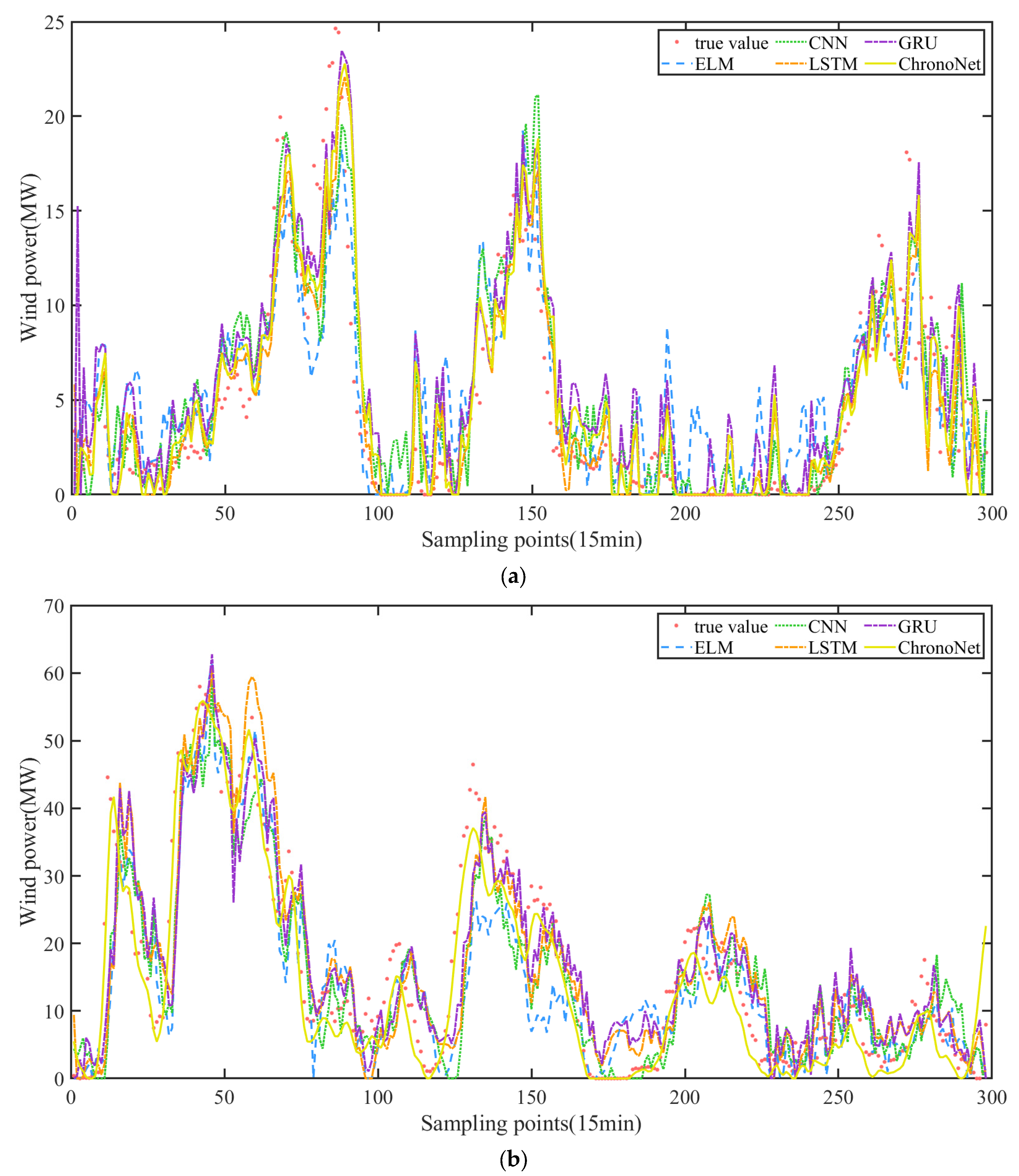
Based on the above parameter settings, the rolling prediction method is adopted in this paper to make deterministic predictions for wind power output one hour in advance, with the results shown in Figure 6.

Firstly, although the ELM can capture the basic trend of wind power output, its predictions exhibit significant fluctuations, indicating limitations in handling the complexity and periodicity of wind power output. The CNN, while sensitive to the extraction of local features, is less effective in capturing the periodicity and regularity of long time series, resulting in relatively rough predictions. LSTM can better capture the long-term dependencies in time-series data, but it still shows some bias when dealing with complex wind power data, especially during periods of high volatility. In contrast, the GRU, although similar to LSTM in capturing time-series regularities, performs slightly worse than LSTM in some complex fluctuations, particularly in long-term predictions. The ChronoNet hybrid model, by combining the strengths of both, can more effectively capture the regularity and volatility of wind power output, showing a significant improvement in prediction accuracy, especially during high-volatility and complex patterns. It can maintain smoothness while accurately reflecting the fluctuation characteristics of wind power.

The deterministic forecasting error metrics of the different models are shown in

Table 4. Comparison of deterministic forecasting metrics.

Season	Prediction Model	RMSE/MW	MAE/MW	R2
Winter	ELM	2.773	2.0151	0.7459
	CNN	2.3437	1.5866	0.8185
	LSTM	2.3252	1.4944	0.8214
	GRU	2.3195	1.5644	0.8223
	BiLSTM	2.2147	1.4783	0.8352
	ChronoNet	2.1334	1.3827	0.8496
Summer	ELM	6.801	4.846	0.7979
	CNN	5.7265	4.0553	0.8567
	LSTM	6.1557	4.5101	0.8344
	GRU	5.5676	4.1332	0.8646
	BiLSTM	4.4538	3.3891	0.9145
	ChronoNet	3.3665	2.6207	0.9505

. Among these metrics, a lower RMSE and MAE indicate smaller prediction errors and better performance, while a higher R² reflects better forecasting performance. As seen from the table, during winter, the ChronoNet model reduces the RMSE by 0.6396 MW, 0.2103 MW, 0.1918 MW, 0.1861 MW, and 0.0813 MW compared to the ELM, CNN, LSTM, GRU, and BiLSTM, respectively. The MAE is reduced by 0.6324 MW, 0.2039 MW, 0.1117 MW, 0.1817 MW, and 0.0956 MW, respectively. R² is increased by 0.1037, 0.0311, 0.0282, 0.0273, and 0.0144, respectively. In summer, the ChronoNet model reduces the RMSE by 3.4345 MW, 2.36 MW, 2.7892 MW, 2.2011 MW, and 1.0873 MW compared to the ELM, CNN, LSTM, GRU, and BiLSTM, respectively. The MAE is reduced by 2.2253 MW, 1.4346 MW, 1.8894 MW, 1.5125 MW, and 0.7684 MW, respectively. R² increases by 0.1526, 0.0938, 0.1161, 0.0859, and 0.036, respectively. Therefore, the ChronoNet model demonstrates a significant advantage in wind power output forecasting, showing stronger adaptability and higher forecasting accuracy.

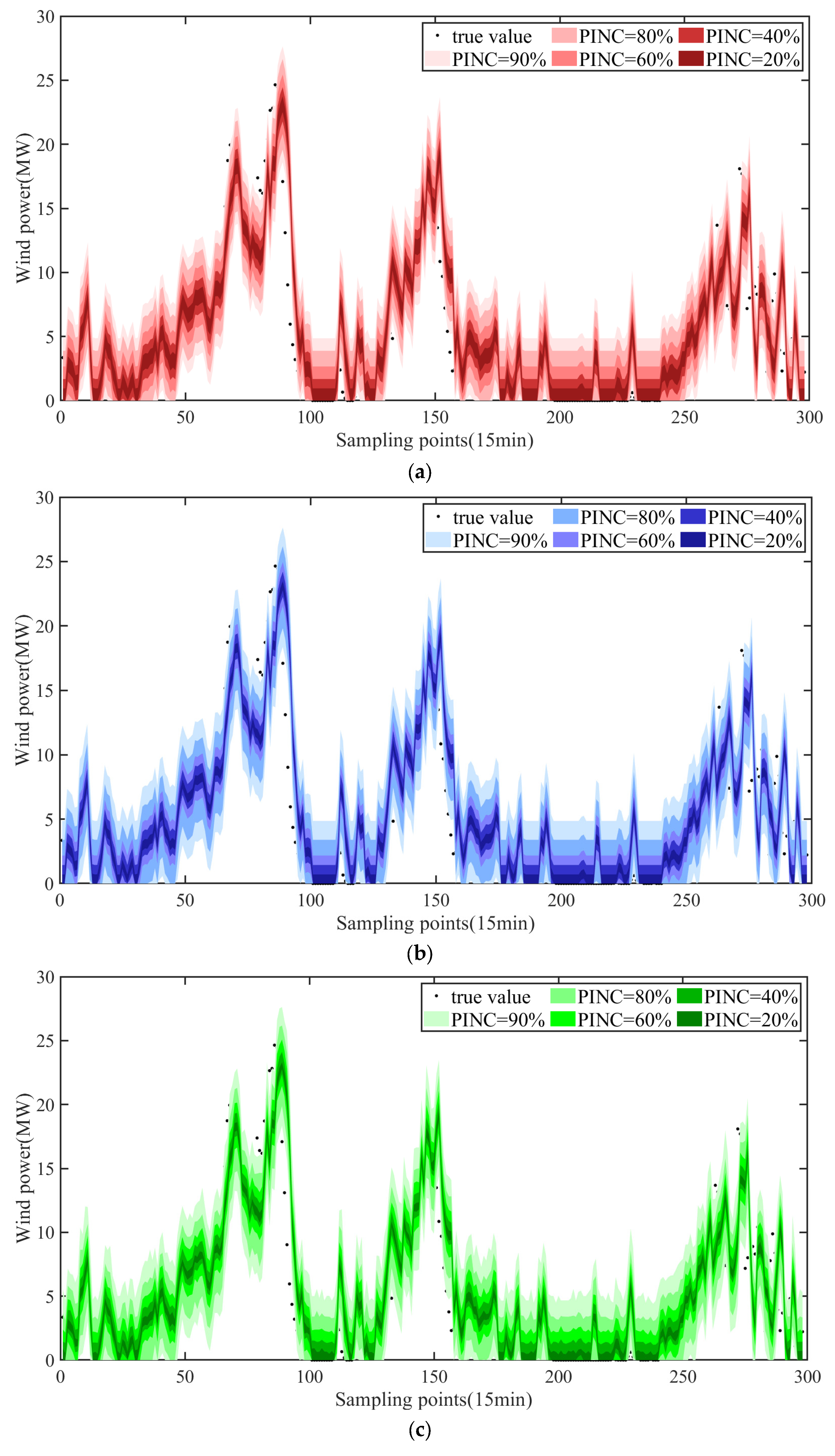
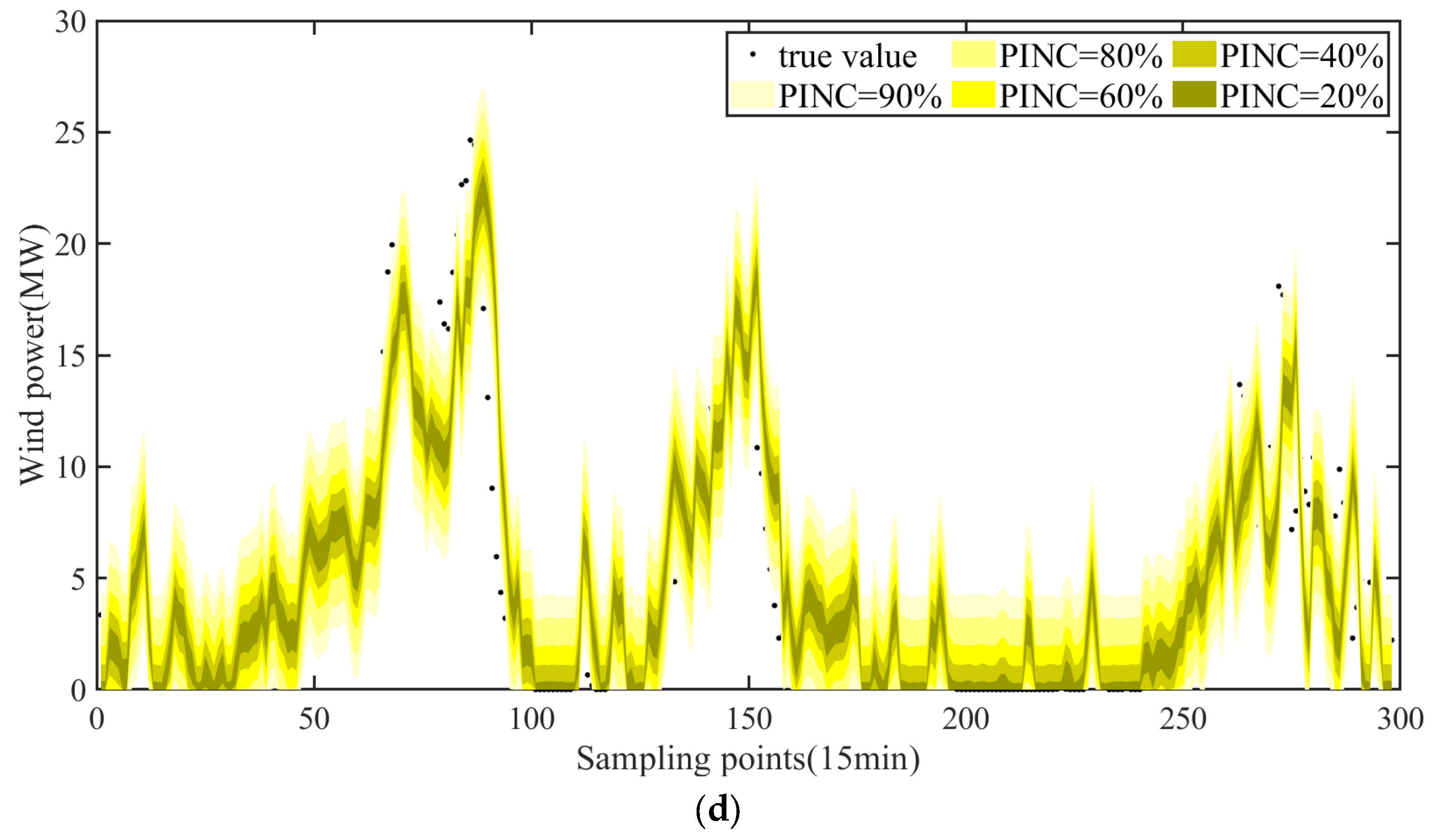
4.3. Probabilistic Forecasting Analysis

The ChronoNet hybrid model can provide accurate deterministic predictions in time-series forecasting. However, in practical applications, the forecast results are often accompanied by uncertainty. Therefore, incorporating probabilistic forecasting analysis can better quantify and assess the uncertainty of predictions, providing decision-makers with more reliable prediction intervals and risk assessments. The probabilistic forecasting results of benchmark methods such as Gaussian distribution, KDE, and Bootstrap resampling are given using winter data as an example. The probabilistic forecasting results of different methods are shown in Figure 7.

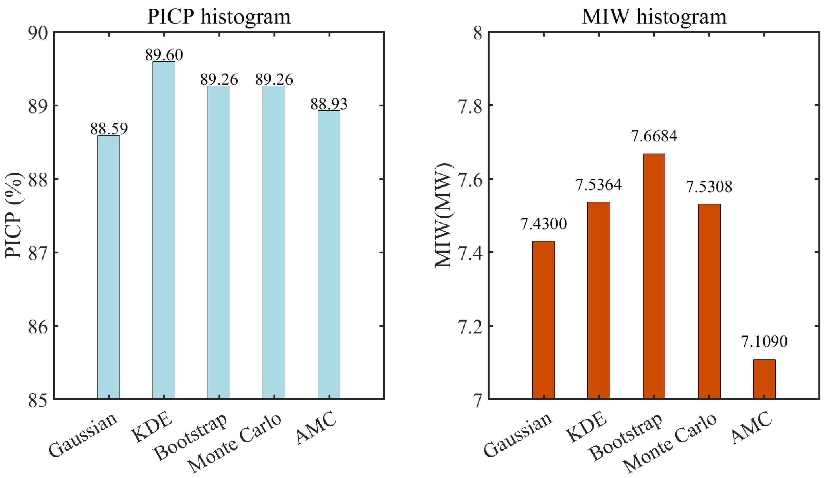
Figure 8 presents the probabilistic prediction metrics for different prediction methods, with PINC = 90% as an example. Specifically, PICP is used to measure the proportion of true values falling within PIs, with higher values indicating better performance. MIW is used to measure the width of the PIs, and smaller MIW values generally suggest more precise predictions. From Figure 8, it can be observed that the difference between the PICP and PINC values of the listed probabilistic forecasting methods is within 2%, indicating that the coverage rates of the various methods are relatively stable and meet the requirements of the given PINC. The advantage of AMC is that its PICP is higher than that of Gaussian distribution, and its MIW is significantly smaller than other methods, reflecting the ability of AMC to effectively model the data distribution and generate more accurate predictions.

To further analyze the probabilistic forecasting performance of different models, the comprehensive metric IS in

Table 5. Comparison of probabilistic comprehensive metrics.

Method	PINC
	20% (IS)	40% (IS)	60% (IS)	80% (IS)	90% (IS)
Gaussian	−7.9823	−7.2682	−5.9245	−3.7821	−2.3131
KDE	−8	−7.4863	−6.1936	−3.8088	−2.2683
Bootstrap	−7.9747	−7.5182	−6.1676	−3.8021	−2.2772
MC	−8.0131	−7.2796	−5.9313	−3.7863	−2.3099
AMC	−7.3232	−6.6983	−5.5307	−3.6068	−2.2017

provides a clear quantitative standard for model performance under different PINC conditions. Specifically, a higher IS represents better overall performance. Compared to the Gaussian, KDE, Bootstrap, and MC methods, at PINC = 20%, the IS of AMC improves by 0.6591, 0.6768, 0.6515, and 0.6899, respectively; at PINC = 40%, the IS of AMC improves by 0.5699, 0.788, 0.8199, and 0.5813; at PINC = 60%, the IS of AMC improves by 0.3938, 0.6629, 0.6369, and 0.4006; at PINC = 80%, the IS of AMC improves by 0.1753, 0.202, 0.1953, and 0.1795; and at PINC = 90%, the IS of AMC improves by 0.1114, 0.0666, 0.0755, and 0.1082.

This result shows that, under different PINC conditions, the AMC method achieves the best IS values. This indicates that AMC method demonstrates strong stability and accuracy in probabilistic forecasting, making it capable of handling complex probabilistic models.

To further compare the effectiveness of the AMC method under different deterministic prediction models,

Table 6. Probabilistic comprehensive metrics of different deterministic prediction models.

Deterministic Method	Probabilistic Method	PINC
		20% (IS)	40% (IS)	60% (IS)	80% (IS)	90% (IS)
CNN-LSTM	MC	−7.4425	−6.7951	−5.6049	−3.6803	−2.2745
	AMC	−7.3379	−6.7194	−5.5525	−3.6433	−2.2583
ChronoNet	MC	−8.0131	−7.2796	−5.9313	−3.7863	−2.3099
	AMC	−7.3232	−6.6983	−5.5307	−3.6068	−2.2017

presents the probabilistic prediction metrics for CNN-LSTM and ChronoNet. In Table 6, the IS of ChronoNet is higher than that of CNN-LSTM under different PINC values, validating the ChronoNet model proposed in this paper is better suited for AMC method.

Additionally, it can be seen that AMC method can better approximate the true probability distribution in the probabilistic prediction process, thereby maintaining stable and efficient performance under various PINC conditions. Therefore, the model proposed in this paper has demonstrated strong adaptability and superiority in probabilistic forecasting tasks, providing strong support for model selection.

5. Conclusions

A MultiFusion–ChronoNet–AMC-based wind power ultra-short-term probabilistic forecasting model is proposed, which can fully demonstrate the advantages of integrating multi-dimensional information and deep learning technologies in modern wind power forecasting. MultiFusion effectively improves the prediction accuracy and robustness of the model by combining meteorological data, geographic information, historical power, and other information, overcoming the limitations of traditional data. The ChronoNet further enhances the model’s ability to handle long-term time-series dependencies and dynamic features. Compared to the traditional LSTM and GRU models, it is better at capturing the complex variation patterns of wind power.

Additionally, compared to the Gaussian distribution, KDE, Bootstrap, and MC methods, the AMC method is more flexible in adapting to nonlinear and high-dimensional complex scenarios, generating more accurate probability distributions and providing more reliable PIs.

In summary, the model proposed in this paper demonstrates stronger adaptability, accuracy, and reliability in wind power forecasting, offering a more efficient decision-support tool for the wind power industry. Future research will focus on ensemble learning and conditional probabilistic prediction of wind farm cluster power, providing strong support for intelligent decision making in the wind energy sector.

References

1. Zhang, L.Y.; Ye, T.L.; Xin, Y.Z.; Han, F.; Fan, G.F. Problems and measures of power grid accommodating large scale wind power. Proc. CSEE 2010, 30, 1–9. [Google Scholar]
2. Famoso, F.; Oliveri, L.M.; Brusca, S.; Chiacchio, F. A Dependability Neural Network Approach for Short-Term Production Estimation of a Wind Power Plant. Energies 2024, 17, 1627. [Google Scholar] [CrossRef]
3. Wan, C.; Song, Y.H. Theories, methodologies and applications of probabilistic forecasting for power systems with renewable energy sources. Autom. Electr. Power Syst. 2021, 45, 2–16. [Google Scholar]
4. Wang, C.; Lin, H.; Yang, M.; Chen, L. Ultra-short-term wind farm cluster interval power prediction based on cluster division and MQ-WaveNet-MSA. Electr. Power Syst. Res. 2025, 244, 111557. [Google Scholar]
5. Cui, Y.; Wang, Y.J.; Huang, Y.H.; Wang, Z.; Wang, M.C. Closed-loop wind power ultra-short-term forecasting strategy based on multi-attention framework and guided supervised learning. Proc. CSEE 2023, 43, 1334–1347. [Google Scholar]
6. Yang, M.; Ju, C.; Huang, Y.; Guo, Y.; Jia, M. Short-term power forecasting of wind farm cluster based on global information adaptive perceptual graph convolution network. IEEE Trans. Sustain. Energy 2024, 15, 2063–2076. [Google Scholar]
7. Yang, M.; Zhang, S.T.; Wang, B. Short-term wind power forecasting method based on a causal regularized extreme learning machine. Power Syst. Prot. Control 2024, 52, 127–136. [Google Scholar]
8. Sun, Y.; Zhou, Q.B.; Sun, L.; Sun, L.P.; Kang, J.C.; Li, H. CNN-LSTM-AM: A power prediction model for offshore wind turbines. Ocean Eng. 2024, 301, 117598. [Google Scholar]
9. Chen, H.P.; Wu, H.; Kan, T.Y.; Zhang, J.H.; Lin, H. Low-carbon economic dispatch of integrated energy system containing electric hydrogen production based on VMD-GRU short-term wind power prediction. Int. J. Electr. Power Energy Syst. 2023, 154, 109420. [Google Scholar]
10. Xue, Y.S.; Lei, X.; Xue, F.; Yu, C.; Dong, Z.Y.; Wen, F.S.; Ju, P. A review on impacts of wind power uncertainties on power systems. Proc. CSEE 2014, 34, 5029–5040. [Google Scholar]
11. Geng, D.H.; Zhang, Y.K.; Zhang, Y.L.; Qu, X.C.; Li, L.F. A hybrid model based on CapSA-VMD-ResNet-GRU-attention mechanism for ultra-short-term and short-term wind speed prediction. Renew. Energy 2025, 240, 122191. [Google Scholar] [CrossRef]
12. Zhou, Y.; Sun, Y.H.; Wang, S.; Bai, L.Q.; Hou, D.C.; Mahfoud, R.J. A very short-term probabilistic prediction method of wind speed based on ALASSO-nonlinear quantile regression and integrated criterion. CSEE J. Power Energy Syst. 2023, 9, 2121–2129. [Google Scholar]
13. Zhou, Y.; Sun, Y.H.; Wang, S.; Mahfoud, R.J.; Alhelou, H.H.; Hatziargyriou, N.; Siano, P. Performance improvement of very short-term prediction intervals for regional wind power based on composite conditional nonlinear quantile regression. J. Mod. Power Syst. Clean Energy 2022, 10, 60–70. [Google Scholar] [CrossRef]
14. Wang, S.; Sun, Y.H.; Zhou, Y.; Wang, J.X.; Hou, D.C.; Zhang, L.C. Ultra-short term conditional probability prediction of wind power considering error time dependence. Electr. Power Autom. Equip. 2022, 42, 40–46. [Google Scholar]
15. Zhu, J.H.; He, Y.Y.; Yang, X.D.; Yang, S.L. Ultra-short-term wind power probabilistic forecasting based on an evolutionary non-crossing multi-output quantile regression deep neural network. Energy Convers. Manag. 2024, 301, 118062. [Google Scholar] [CrossRef]
16. Dong, W.C.; Sun, H.X.; Tan, J.X.; Li, Z.; Zhang, J.X.; Yang, H.F. Regional wind power probabilistic forecasting based on an improved kernel density estimation, regular vine copulas, and ensemble learning. Energy 2022, 38, 122045. [Google Scholar] [CrossRef]
17. Xiao, L.; Li, M.T.; Zhang, S.H. Short-term power load interval forecasting based on nonparametric Bootstrap errors sampling. Energy Rep. 2022, 8, 6672–6686. [Google Scholar] [CrossRef]
18. Wei, Q.; Tang, Z.J. Wind power range prediction based on SSA-VMD-SE-KELM combined with Monte Carlo method. Smart Power 2022, 50, 59–66. [Google Scholar]
19. Yang, M.; Dong, H. Short-term wind power interval prediction based on wind speed of numerical weather prediction and Monte Carlo method. Autom. Electr. Power Syst. 2021, 45, 79–85. [Google Scholar]
20. Sun, R.F.; Zhang, T.; He, Q.; Xu, H.X. Review on key technologies and applications in wind power forecasting. High Volt. Eng. 2021, 47, 1129–1143. [Google Scholar]
21. Wang, Y.Y.; Shen, R.J.; Ma, M. Research on ultra-short term forecasting technology of wind power output based on various meteorological factors. Energy Rep. 2022, 8, 1145–1158. [Google Scholar]
22. Lu, P.; Ye, L.; Pei, M.; Zhao, Y.N.; Dai, B.H.; Li, Z. Short-term wind power forecasting based on meteorological feature extraction and optimization strategy. Renew. Energy 2022, 184, 642–661. [Google Scholar] [CrossRef]
23. Mo, Y.P.; Wang, H.X.; Yang, C.T.; Yao, Z.H.; Li, B.X.; Fan, S.H.; Mo, S. FDNet: Frequency filter enhanced dual LSTM network for wind power forecasting. Energy 2024, 312, 133514. [Google Scholar]
24. Yang, X.Y.; Liu, Y.Q.; Li, J.L. Reliability confidence interval calculation method for photovoltaic power station with energy storage based on quartile method. Trans. China Electrotech. Soc. 2017, 32, 136–144. [Google Scholar]
25. Rameshrao, A.G.; Koley, E.; Ghosh, S. Reliability enhancement of hybrid microgrid protection against communication data loss and converter faults using cubic-spline interpolation, Savitzky Golay filtering and GRU network. Comput. Electr. Eng. 2024, 116, 109144. [Google Scholar]
26. Wang, S.; Zhang, W.J.; Sun, Y.H.; Trivedi, A.; Chung, C.Y.; Srinivasan, D. Wind power forecasting in the presence of data scarcity: A very short-term conditional probabilistic modeling framework. Energy 2024, 291, 130305. [Google Scholar] [CrossRef]
27. Cai, C.H.; Zhang, L.Y.; Zhou, J.G. DMPR: A novel wind speed forecasting model based on optimized decomposition, multi-objective feature selection, and patch-based RNN. Energy 2024, 310, 133277. [Google Scholar] [CrossRef]
28. Wang, L.X.; Dong, H.L.; Cao, Y.Q.; Hou, D.B.; Zhang, G.X. Real-time water quality detection based on fluctuation feature analysis with the LSTM model. J. Hydroinform. 2023, 25, 140–149. [Google Scholar] [CrossRef]
29. Xiao, Y.L.; Zou, C.Z.; Chi, H.T.; Fang, R.C. Boosted GRU model for short-term forecasting of wind power with feature-weighted principal component analysis. Energy 2023, 267, 126503. [Google Scholar]
30. Deng, J.W.; Xiao, Z.; Zhao, Q.C.; Zhan, J.; Tao, J.; Liu, M.H.; Song, D.R. Wind turbine short-term power forecasting method based on hybrid probabilistic neural network. Energy 2024, 313, 134042. [Google Scholar]
31. Pegg, K.; Wilson, G.; Al-Duri, B. Exploring Trigeneration in MSW Gasification: An Energy Recovery Potential Study Using Monte Carlo Simulation. Energies 2025, 18, 1034. [Google Scholar] [CrossRef]
32. Kou, B.Y.; Zhang, Y.; Ma, F.L. The applications of central limit theorem. J. Sci. Teach. Coll. Univ. 2019, 39, 53–56. [Google Scholar]
33. Chen, Y.J.; Xiao, J.W.; Wang, Y.W.; Luo, Y.F. Non-crossing quantile probabilistic forecasting of cluster wind power considering spatio-temporal correlation. Appl. Energy 2025, 377, 124356. [Google Scholar]
34. Zhou, Y.; Wei, F.Z.; Kuang, K.Y.; Mahfoud, R.J. Research on a deep ensemble learning model for the ultra-short-term probabilistic prediction of wind power. Electronics 2024, 13, 475. [Google Scholar] [CrossRef]
Figure 1. Principle of multi-source data fusion.
Energies 18 01646 g001
Figure 2. ChronoNet structure.
Energies 18 01646 g002
Figure 3. Flowchart of the hybrid forecasting model.
Energies 18 01646 g003
Figure 4. Data preprocessing results: (a) before cleaning and (b) after cleaning.
Energies 18 01646 g004
Figure 5. Correlation coefficient heatmaps: (a) Pearson; (b) Kendall; and (c) Spearman.
Energies 18 01646 g005
Figure 6. Deterministic forecasting results: (a) winter and (b) summer.
Energies 18 01646 g006
Figure 7. Probabilistic forecasting results: (a) Gaussian; (b) KDE; (c) Bootstrap; and (d) AMC.
Energies 18 01646 g007aEnergies 18 01646 g007b
Figure 8. Bar chart of probabilistic predictive metrics.
Energies 18 01646 g008