Wireless Power Transfer Optimization with a Minimalist Single-Capacitor Design for Battery Charging

Abstract

Along with the emerging needs to either complement or replace the limitation of energy storage technologies in batteries in supplying power to mobile devices, including electric vehicles, Wireless Power Transfer (WPT) technologies are becoming the main focus to solve this problem. However, much research is still in progress in relation to how to achieve high power delivery from the transmitter to the receiver of the WPT circuit. Since most research that has been done tends to add components or circuits so that the system becomes more complex, this study proposes the optimization design of a single capacitor on the WPT transmitter side due to the fact that the presence of the rectifier circuits guarantees the existence of a capacitance characteristic on the receiver side. Using a full bridge rectifier to represent the WPT load, a mathematical model of the overall system is then built based on state space and transfer function methods. Then, a Genetic Algorithm (GA) is applied to the model to find the optimum solutions for achieving high power delivery. Here, the WPT power output to the load is chosen as the fitness function, while the constraints are the available capacitance and voltage source frequency values. A case study with MATLAB R2024b simulation shows that the proposed method successfully delivers the highest possible power transfer delivery, which is around 0.1 watts using a normalized AC voltage source amplitude of 1 volt. This power will increase if the voltage source amplitude is increased. In addition, the results of the GA sensitivity test ensure the consistency of the optimization results.

1. Introduction

Currently, electronic circuits and devices have reached an era where they are widely used in the form of mobile devices, which have smaller sizes and high efficiency [1,2]. These include not only the small ones, for example, biomedical devices [3], but also big-sized devices, such as Electric Vehicles (EVs) [4]. EVs are gaining popularity and high encouragement in many governmental policies related to their contributions in replacing the fossil-fueled vehicles that have a negative impact on environmental sustainability.

These mobile devices, related to their power supply, highly depend on batteries. Ironically, related to the previous mentioned motivation, this causes a heavy concern associated with environmental damage and sustainability [5]. Moreover, the current energy storage technology in batteries is still not mature enough to mitigate those issues [6,7]. Here, wireless power transfer (WPT) provides a reliable alternative solution to power those devices [8,9].

Generally, compared to conventional charging methods, i.e., wired power transfer, WPT is superior. Since it does not need physical connections, it is more convenient. Hence, it is easier to use and increases usage mobility [10]. Moreover, related to the elimination of physical connectors, this means less wear and tear on devices and cables [11], lower material costs [12,13], lower risk of electrocution [14], and enabling new design possibilities, e.g., waterproof devices [15,16,17]. Also, fewer cables means less clutter, a more organized environment [18], and easier integration into a wide range of applications [10]. All of these benefits cause WPT to be used in many fields in addition to mobile device charging purposes [19,20], for example, in medicine [21,22]. On the other hand, WPT is also a solution for conditions where it is impossible to use wired connections, for example, in mining or underwater operations [23,24,25].

Actually, even though WPT technology has become a trend in research and development recently to complement the limitation in battery energy storage technology advancement, the foresight about it had already happened long ago, which was started by Nikola Tesla in 1891 [26,27]. It started to gain attention again in 2007 after some MIT scientists succeeded in lighting a 60 W bulb from a distance of 2 m [28].

Using a top-down approach, WPT can be categorized into two types: far-field WPT and near-field WPT. Furthermore, far-field WPT consists of Microwave Power Transfer (MPT) and Laser Power Transfer (LPT) [29,30,31,32,33]. On the other hand, near-field WPT consists of Inductive Power Transfer (IPT) and Capacitive Power Transfer (CPT) [34]. Since far-field WPT uses a radioactive method to transfer energy or power, its use is limited to specific needs, such as powering satellites or unmanned ships. Hence, for mobile electric circuits or devices, near-field WPT which uses a nonradioactive method, is chosen [13,35].

In the case of near-field WPT, IPT and CPT differ on how the power is transferred. In IPT, it is transferred via a magnetic field, while in CPT, it is transferred via an electric field [36,37,38]. Thus, there are two coils, each placed in the transmitter (primary) and the receiver (secondary) side in IPT. On the other hand, CPT uses two metal plates, each in the transmitter and the receiver, that act as electrodes like in the capacitor. Thus, IPT is often also called inductive coupling WPT, while CPT is called capacitive coupling WPT [39,40,41].

Currently, the advancement in CPT development is still underperformed by IPT in the case of power transfer distance, where it is not capable of transmitting power farther than 100 mm compared to IPT that is able to transmit in the range of cm to m [42]. Since our study is part of the examination of wireless power transfer to charge mobile device batteries, we chose to concentrate more on how to contribute to the development of IPT. Thus, from here on, we use the WPT term in referring to the IPT WPT technology for the sake of convenience.

IPT WPT technology can be categorized into two types: inductive coupled wireless power transfer and magnetically coupled resonance wireless power transfer [10]. Their difference lies only in how to increase the efficiency of the transmitted power, where the resonance frequency plays an important role in the latter [28,43,44,45]. Hence, the existence of capacitors is an easy indicator to say that an IPT circuit applies the magnetic resonance approach.

Unfortunately, in reality, the implementation to achieve the best efficiency using the resonance phenomenon is not as simple as it seems. Even though placing a capacitor with an appropriate capacitance value at each circuit that contains a coil (inductor) can always generate resonance, the best efficiency can only be obtained through many electric circuit analysis. Thus, many compensating techniques are proposed through many conducted studies, such as Series-Series (SS), Series-Parallel (SP), Parallel-Series (PS), or Parallel-Parallel (PP) compensation networks [46]. Research to study the effect of the number of coils has also been done for this purpose [9]. In addition, a relation of the shape of the coils to the power transfer efficiency has also been presented by [47]. Still related to it, a study by [48] showed that a star-shaped coil in the WPT transmitter can increase the power transfer efficiency in spite of rotation and misalignment on the receiver side. On the other hand, Ref. [24] showed that the distance between coils also heavily influences the efficiency. Moreover, a recent study [49] showed that an optimal frequency selection can be applied to improve the power transfer in tightly coupled WPT systems instead of the inherent resonant frequency.

Apart from the efficiency issue, in the case of WPT for EV charging purposes, safety is also an important consideration. Since inefficiency can cause a temperature rise in the ground assembly surface, it needs to be evaluated, which has been done in [50]. Other than that, ref. [51] has proposed a metal object detection method to reduce the risk of device charging damage.

In contrast to the previous approaches, where they tend to add components or make the circuit more complex, ref. [52] proposed to add only a single capacitor on the transmitter side, where a high output power transfer is achieved through an optimization process using mathematical approaches. Thus, this approach has the potential to have advantages in terms of lower costs. Moreover, since the end goal of our research is WPT optimization design in charging batteries regardless of the load, this single-capacitor approach on the transmitter side is reasonable because a capacitance characteristic is guaranteed to exist on the WPT receiver side due to the presence of the rectifier circuit. Hence, the interoperability demands are still fulfilled [53]. In addition, the objective is aligned with the need to achieve an optimum battery charging performance, even in the presence of unexpected load [54].

Still, the load has only been modeled as a simple resistor in the said previous research [52], while mathematical equations show that the power output depends on the load. Here, in this study, we aim to improve it by using a more realistic load representation. Moreover, along with the current phenomenon where Artificial Intelligence (AI) has been widely available and easy to use, the implementation of the Genetic Algorithm to find the optimum solution is discussed. Generally, the GA is chosen because of its proven performance in solving many problems in WPT [55,56,57]. Specifically, the GA is selected because, by using our proposed method, the objective function (fitness function) is easily defined, along with the boundary conditions (constraints).

Research Aims: Commonly, some primary challenges in WPT now revolve around its efficiency, safety, power delivery distance, environmental interference, security, and design or fabrication considerations [13,37,58,59]. As mentioned earlier, where many solution offerings tend to add components, thus increasing the complexity of the system, we sought to investigate how a simple single-capacitor circuit could be optimized to improve the performance of WPT for mobile device battery charging purposes. Our study conducted here offers preliminary theoretical research in achieving the possible highest power transfer before addressing the efficiency and hardware implementation investigation. This preceding investigation on high power transfer before efficiency is acceptable because efficiency has no direct relation with power, i.e., efficiency is not always maximum when either power in the WPT transmitter and receiver is maximum [60].

Specifically, the research questions that are presented in this study are the following:

• How to model a realistic load for WPT with an objective to charge mobile device batteries?
• Using the previous load, how to mathematically model the WPT power output?
• Based on the previous model, how to choose the optimization parameters for the WPT power output?
• How to apply the GA in finding the optimum model’s parameters?

The structure of this paper is as follows: Section 2 gives a brief explanation about the state space and transfer function methods used for system modeling. Section 3 presents a WPT mathematical modeling approach. Section 4 is dedicated to discussing our WPT load modeling approach. Section 5 discusses the optimization of the system consisting of a WPT circuit and the load. Section 6 verifies and validates the proposed method using a simulated case study. Also, the implementation of the GA is explained there. Section 7 summarizes the results and also presents further works of this study.

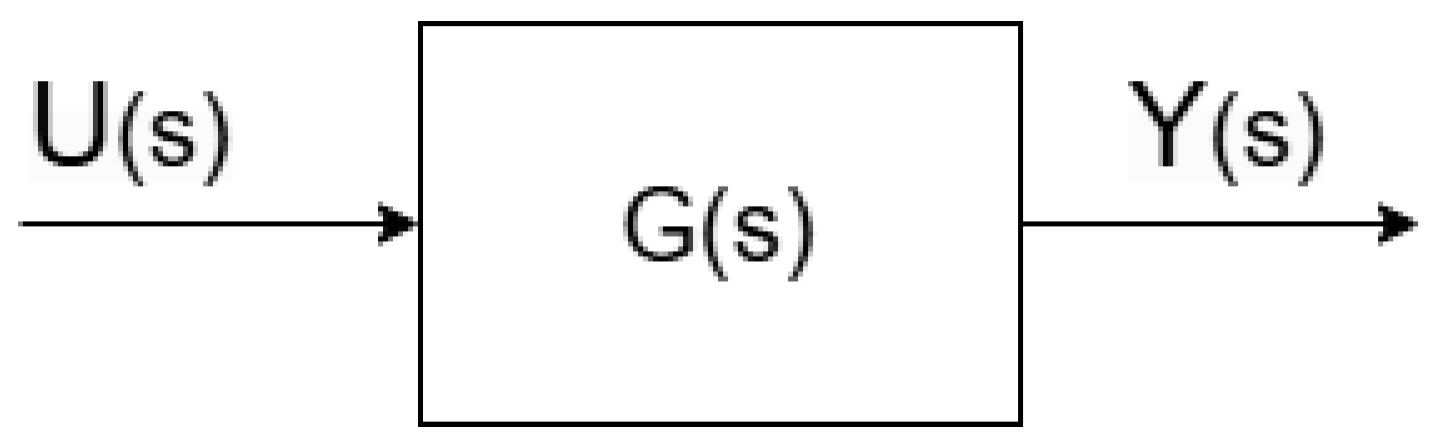
2. State Space and Transfer Function

In this study, state space and transfer function methods are chosen as tools in modeling the system. First, from system dynamics differential equations, a state space mathematical model is built. State space is selected because its representation is in the form of a set of matrix equations so that many relations among electrical signals can be expressed [61,62]. Further on, it can also be used to represent systems with multiple inputs and multiple outputs [63]. However, since it is a time-domain-based system model, the transfer function method is then used to transform it into the domain of frequency [64,65,66]. This is preferred because the electric source signal in the WPT system is AC. This section gives a brief discussion about the state space and transfer function methods.

2.1. State Space System Model Representation

In system and control theory, it is common to describe the relationship between the system input and output variables in the form of differential equations where the time evolution of the internal system states, called state variables, depends on their values at a given time instant [67]. In this state space representation, the outputs represent the measured state variables, while the inputs represent either the system’s sources or the control vector. In more general cases, the disturbance from the environment can also be included in the system inputs. Hence, since the WPT system equations can be written in differential equations form, this state space representation is suitable for modeling it.

If the considered system is Linear Time Invariant (LTI) and finite-dimensional, then the state space representation can be written in the form of a set of matrix equations [68,69]. Thus, it also benefited in terms of its ability to describe a Multiple Input Multiple Output (MIMO) system. If the system is nonlinear, under some assumptions, a preceding linearization process can be carried out before forming the state space model [70].

Consider a nonlinear system as follows:

$$\begin{array}{c}\hfill \begin{array}{cc}\hfill {\displaystyle \frac{dx}{dt}}=\dot{x}& =f(x,u),x\left(t_0\right)=x_0\hfill \\ \hfill y& =g(x,u)\hfill \end{array}\end{array}$$

(1)

where $x\in {\mathbb{R}}^n$ is the system’s state variables, $x_0$ is the states’ initial conditions, $u\in {\mathbb{R}}^r$ is the system’s input, and $y\in {\mathbb{R}}^m$ is the measured system’s output. f and g should be derivable.

Then, for a small displacement of $\Delta x=x-x_{eq}$ and $\Delta u=u-u_{eq}$ around $(x_{eq},u_{eq}$, where $f(x_{eq},u_{eq})=0$, Equation (1) can be linearized using the Taylor series expansion, where the higher-order terms can be neglected by assuming that their values are small. Meanwhile, for the lower-order terms, it can be computed by doing a partial derivative at $(x_{eq},u_{eq})$. This first-order partial derivative gives the Jacobian matrix. Thus, the linearization process can be written as follows:

$$\begin{array}{c}\hfill \begin{array}{cc}\hfill f(x_{eq}+\Delta x,u_{eq}+\Delta u)& =f(x_{eq},u_{eq})+\underset{A_s}{\underbrace{{\displaystyle \frac{df}{dx}}{|}_{(x_{eq},u_{eq})}}}\Delta x+\underset{B_s}{\underbrace{{\displaystyle \frac{df}{du}}{|}_{(x_{eq},u_{eq})}}}\Delta u\hfill \\ \hfill g(x_{eq}+\Delta x,u_{eq}+\Delta u)& =g(x_{eq},u_{eq})+\underset{C_s}{\underbrace{{\displaystyle \frac{dg}{dx}}{|}_{(x_{eq},u_{eq})}}}\Delta x+\underset{D_s}{\underbrace{{\displaystyle \frac{dg}{du}}{|}_{(x_{eq},u_{eq})}}}\Delta u\hfill \end{array}\end{array}$$

(2)

where $A_s$, $B_s$, $C_s$, and $D_s$ are the Jacobian matrices with appropriate dimensions.

Then, by shifting $(x_{eq},u_{eq})$ to $(0,0)$ (the origin point) and dropping $\Delta$, we can obtain the linearized model as follows:

$$\begin{array}{c}\hfill \begin{array}{cc}\hfill {\displaystyle \frac{dx}{dt}}=\dot{x}& =A_{s}x+B_{s}u,x\left(t_0\right)=x_0\hfill \\ \hfill y& =C_{s}x+D_{s}u\hfill \end{array}\end{array}$$

(3)

Hence, the general LTI system model in a state space form is shown in Equation (3).

2.2. Transfer Function System Model Representation

The previous system state space representation is a time domain approach, since it is derived from the time evolution of the system state variables. On the other hand, since the WPT power transfer delivery utilizes an induction phenomenon generated from an AC voltage source, it is highly desired to describe the WPT system in the frequency domain. Fortunately, a transformation coordinate process from the time domain to the frequency domain can be done by using the Laplace transformation [71,72], which is defined as follows:

$$F\left(s\right)=\mathcal{L}\left[f\left(t\right)\right]={\int }_0^{\infty }f\left(t\right)e^{-st}dt$$

(4)

where $\mathcal{L}$ is the Laplace transform operator, and $s\in \mathcal{C}$ is the Laplace transform complex variable.

This Laplace transform operation can be considered a time–frequency coordinate transformation because, formally, s can be substituted into $s=i\omega$ to describe the relation between the Laplace and Fourier transformations. In some cases, s can also be treated as a complex variable $s=\alpha +i\omega$ in order to describe a possible exponential characteristic contained in a function.

Further on, there is a property in the Laplace transform that is defined as follows:

$$\mathcal{L}\left[{\displaystyle \frac{df\left(t\right)}{dt}}\right]=sF\left(s\right)-f\left(0\right)$$

(5)

where $F\left(s\right)=\mathcal{L}\left[f\right(t\left)\right]$.

If we utilize Equation (5) in Equation (3) by assuming zero initial conditions, then it can be obtained that

$$\begin{array}{c}\hfill \begin{array}{cc}\hfill sX\left(s\right)& =A_{s}X\left(s\right)+B_{s}U\left(s\right)\hfill \\ \hfill Y\left(s\right)& =C_{x}X\left(s\right)+D_{s}U\left(s\right)\hfill \\ \hfill Y\left(s\right)& =[C_s{(sI-A_s)}^{-1}{B}_s+D_s]U\left(s\right)\hfill \end{array}\end{array}$$

(6)

where I is the identity matrix with appropriate dimension, $X\left(s\right)=\mathcal{L}\left[x\right(t\left)\right]$ is the system’s state variables in the Laplace transform domain, $Y\left(s\right)=\mathcal{L}\left[y\right(t\left)\right]$ is the system’s output in the Laplace transform domain, and $U\left(s\right)=\mathcal{L}\left[u\right(t\left)\right]$ is the system’s input in the Laplace transform domain.

A system transfer function is defined as a mathematical model that relates the system’s input to the system’s output, usually in the complex Laplace variable domain s [73,74], as seen in Figure 1.

Hence, based on Equation (6) and Figure 1, a system transfer function $G\left(s\right)$ from a general state space representation seen in Equation (3) can be written as follows:

$${\displaystyle \frac{Y\left(s\right)}{U\left(s\right)}}=G\left(s\right)=C_s{(sI-A_s)}^{-1}{B}_s+D_s$$

(7)

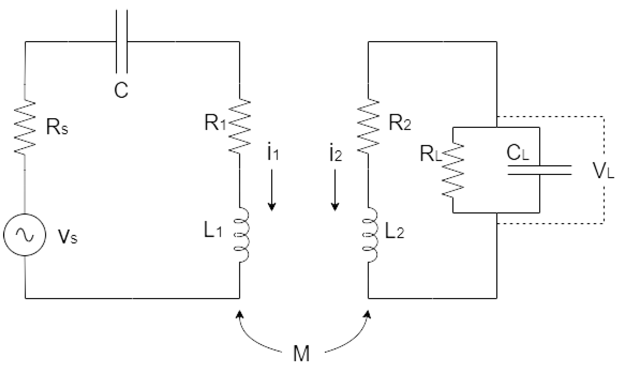
3. The Single-Capacitor WPT Modeling

In its simplest form, the WPT circuit consists of two inductors, where one is on the transmitter side, while the other is on the receiver side. An Alternating Current (AC) source is then connected to the inductor on the transmitter side. Thus, the power is delivered from the transmitter via a magnetic field to generate an induction on the receiver side where a load is attached.

Since the existence of an inductor in an electrical circuit causes a phase shift between the voltage and the current, it is common to add a capacitor to counteract the effect so that the active power is increased. Generally, because there are two inductors, two capacitors are added, where their capacitance values are determined by using resonance frequency calculation in each of the transmitter and receiver circuits. However, by assuming that the WPT optimization end goal in charging batteries should be achieved regardless of the load, it is accepted to assume that the manipulable capacitor is the one that is attached to the WPT transmitter side. In addition, a capacitor can be assumed to always exist on the WPT receiver side due to the presence of a rectifier circuit in the WPT load.

From here on, we refer to the transmitter circuit as the primary circuit and the receiver circuit as the secondary circuit. In addition, the inductors are referred to as coils.

Consider a single-capacitor WPT circuit diagram as shown in Figure 2, where $V_s$ is the voltage source, $R_s$ is the source resistance, C is the primary capacitance, $R_1$ is the primary coil resistance, $L_1$ is the primary coil inductance, $R_2$ is the secondary coil resistance, $L_2$ is the secondary coil inductance, $V_L$ is the secondary circuit output voltage, $i_1$ is the current in the primary circuit, and $i_2$ is the current in the secondary circuit.

In addition, M is the mutual inductance between both coils, which is defined as follows:

$$M=K\sqrt{L_1{L}_2}$$

(8)

where $0<K<1$ is called the coupling coefficient.

Then, by using the Kirchhoff Law, we can derive some equations as follows:

$$\begin{array}{c}\hfill \begin{array}{cc}\hfill V_s& =i_1{R}_s+V_c+i_1{R}_1+L_1{\displaystyle \frac{d{i}_1}{dt}}+M{\displaystyle \frac{d{i}_2}{dt}}\hfill \\ \hfill 0& =i_2{R}_2+L_2{\displaystyle \frac{d{i}_2}{dt}}+M{\displaystyle \frac{d{i}_1}{dt}}+V_L\hfill \\ \hfill V_C& ={\displaystyle \frac{1}{C}}\int i_{1}dt\hfill \end{array}\end{array}$$

(9)

where $V_C$ is the capacitor voltage.

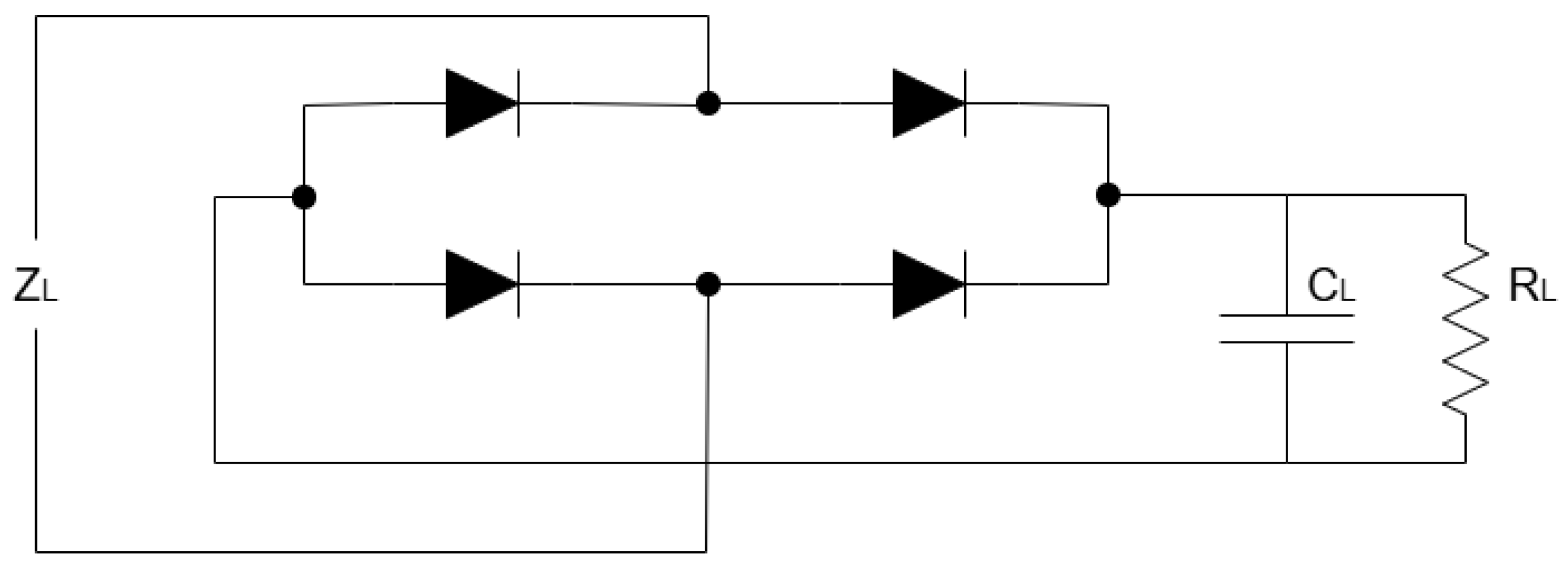
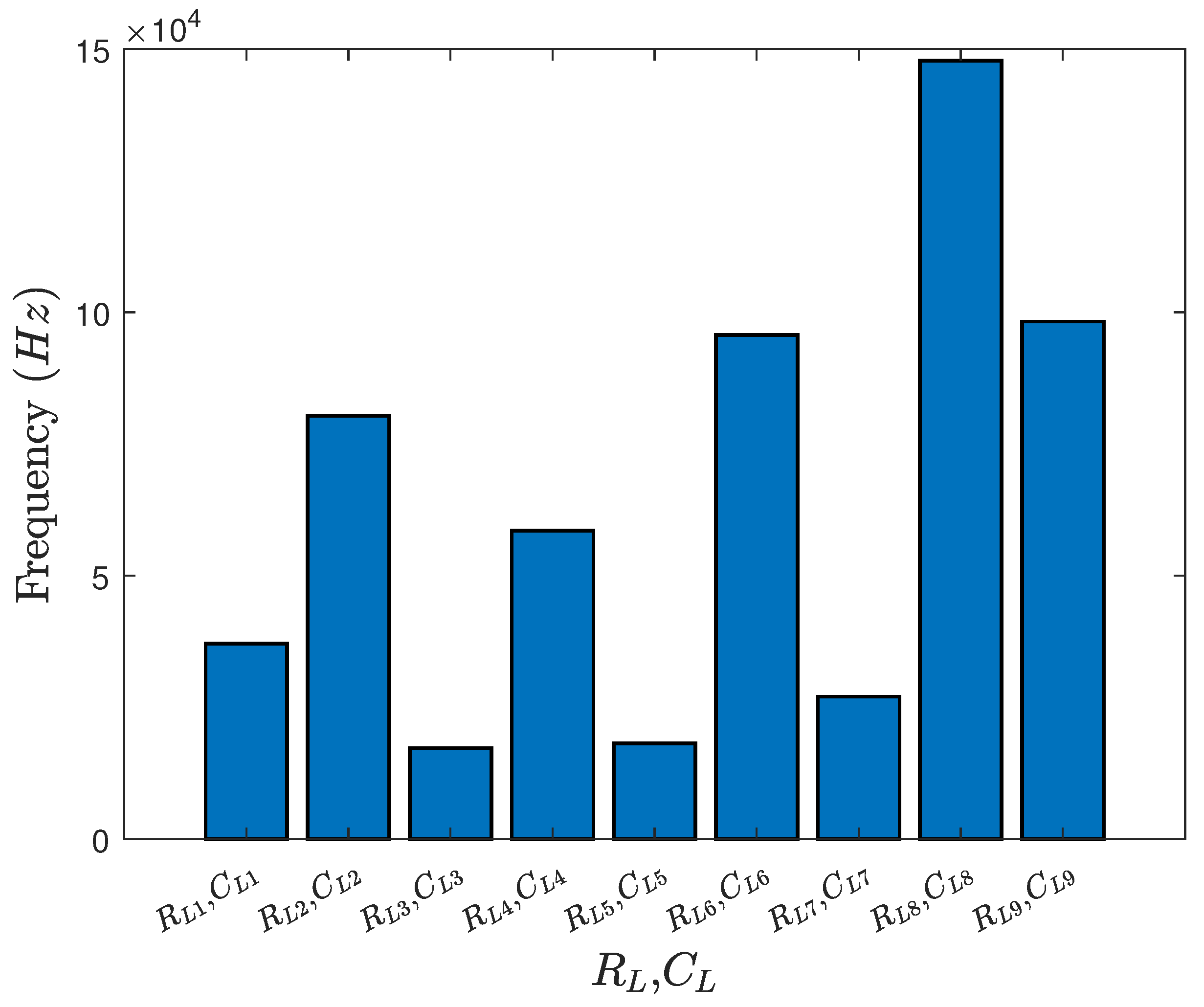
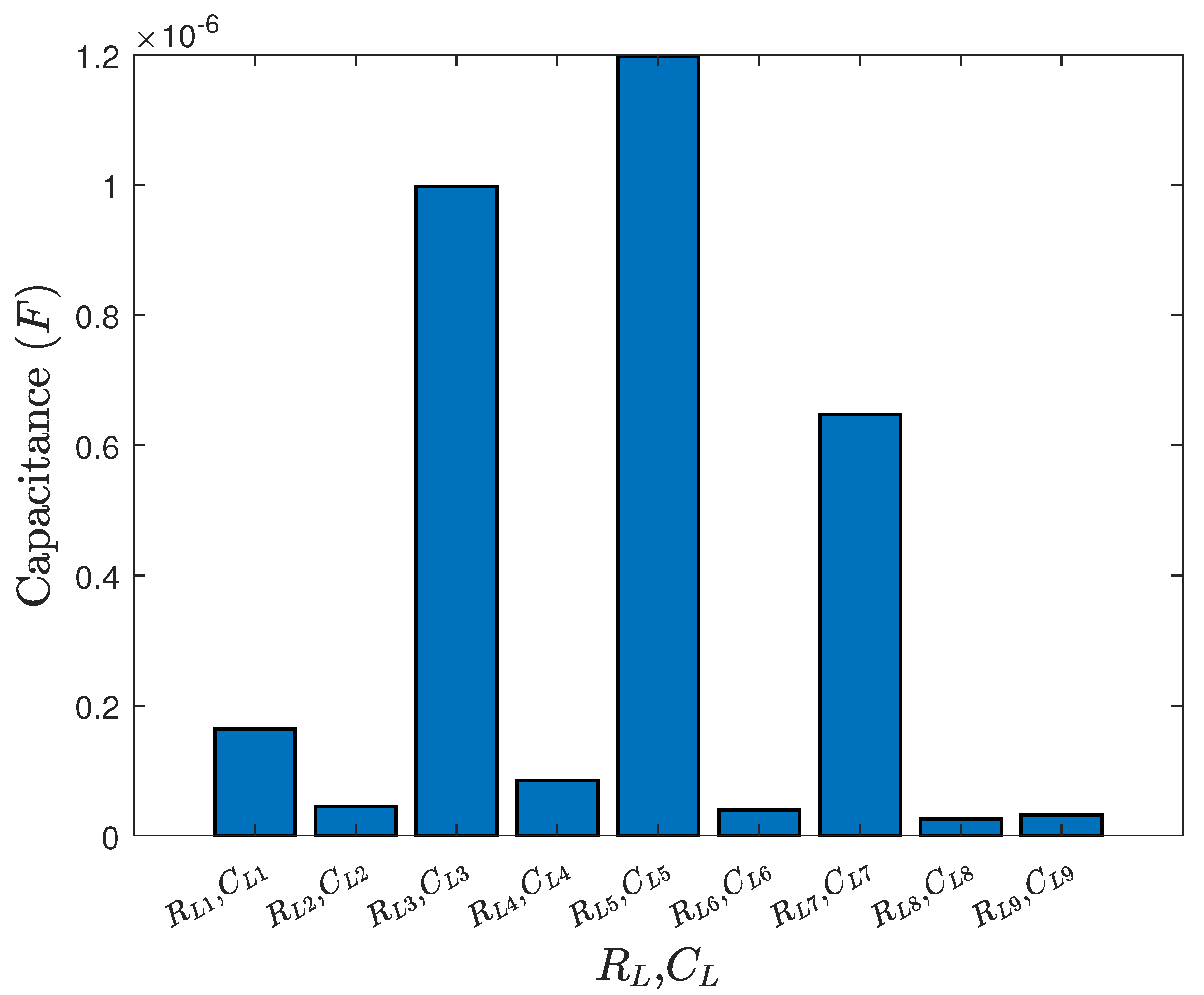
4. WPT Load Modeling

In this study, the WPT’s objective is to be used as a charging station for some mobile electronic device batteries. For this purpose, some standards, for example, the Qi standard [75,76,77] or the Airfuel standard [78], already exist where low frequencies are chosen. Further on, a rectifier circuit is needed to change the AC form of the electrical quantities from the WPT into Direct Current (DC) form before being supplied to the mobile devices. Some previous studies show that a full bridge rectifier circuit is good enough to represent the load in the WPT system under low-frequency operating conditions [79,80,81]. Therefore, in our study, the load on the secondary side of the WPT is assumed to be a full bridge rectifier.

The considered electrical circuit of this rectifier, using four diodes, is shown in Figure 3, where $C_L$ is the load capacitance, $R_L$ is the load resistance, and $Z_L$ is the load impedance viewed from the load connectors.

Since our objective is optimizing the WPT circuit to deliver the highest possible power transfer regardless of the load, we are interested in modeling the load impedance of the rectifier. Hence, the diodes are then replaced by resistors to represent their resistance, as shown in Figure 4, where $R_{Dk}$ is the resistance of the kth diode.

Furthermore, the values of $R_{Dk}$ are assumed to be zero because they are usually small enough compared to the other electrical component parameter values. Thus, the rectifier circuit is simplified to an RC parallel circuit, as shown in Figure 5, where $V_L$ is the load voltage, $i_L$ is the electric current going out and in the load voltage, $i_{CL}$ is the electric current going through $C_L$, and $i_{RL}$ is the electric current going through $R_L$.

Then, by using the Kirchhoff Law, some equations for the RC parallel circuit are derived as follows:

$$\begin{array}{c}\hfill \begin{array}{cc}\hfill i_{CL}& =C_L{\displaystyle \frac{d{V}_L}{dt}}\hfill \\ \hfill i_{RL}& ={\displaystyle \frac{V_L}{R_L}}\hfill \\ \hfill i_L& =i_{CL}+i_{RL}\hfill \\ \hfill V_L& =i_L{Z}_L\hfill \end{array}\end{array}$$

(10)

where $Z_L$ is the impedance of the load that is attached to the secondary circuit.

5. System Modeling and Optimization

As mentioned previously, the full bridge rectifier is assumed to be the load on the secondary side of the WPT. Thus, the full system circuit becomes as shown in Figure 6.

By combining Equations (9) and (10), the system state space can be written in the form of Equation (3) as follows:

$$\begin{array}{c}\hfill \begin{array}{cc}\hfill \dot{x_s}& =A_s{x}_s+B_s{u}_s\hfill \\ \hfill y_s& =C_s{x}_s+D_s{u}_s\hfill \\ \hfill x_s& ={\left[\begin{array}{cccc}{V}_c& V_L& i_1& i_2\end{array}\right]}^T,u_s=V_s,y_s=V_L\hfill \\ \hfill A_s& =\left[\begin{array}{cccc}0& 0& {\displaystyle \frac{1}{C}}& 0\\ 0& {\displaystyle \frac{-1}{C_L{R}_L}}& 0& {\displaystyle \frac{1}{C_L}}\\ {\displaystyle \frac{L_2}{M^2-L_1{L}_2}}& {\displaystyle \frac{-M}{M^2-L_1{L}_2}}& {\displaystyle \frac{L_2{R}_1+L_2{R}_s}{M^2-L_1{L}_2}}& {\displaystyle \frac{-M{R}_2}{M^2-L_1{L}_2}}\\ {\displaystyle \frac{-M}{M^2-L_1{L}_2}}& {\displaystyle \frac{L_1}{M^2-L_1{L}_2}}& {\displaystyle \frac{-M{R}_1-M{R}_s}{M^2-L_1{L}_2}}& {\displaystyle \frac{L_1{R}_2}{M^2-L_1{L}_2}}\end{array}\right]\hfill \\ \hfill B_s& =\left[\begin{array}{c}0\\ 0\\ {\displaystyle \frac{-L_2}{M^2-L_1{L}_2}}\\ {\displaystyle \frac{M}{M^2-L_1{L}_2}}\end{array}\right],C_s=\left[\begin{array}{cccc}0& 1& 0& 0\end{array}\right],D_s=\left[\begin{array}{c}0\\ 0\end{array}\right]\hfill \end{array}\end{array}$$

(11)

Then, the system transfer function $G\left(s\right)$ can be obtained from the state space in Equation (11) by the relation described in Equation (7) as follows:

$$\begin{array}{c}\hfill \begin{array}{cc}\hfill G\left(s\right)=& {\displaystyle \frac{\mathcal{L}\left[y_s\left(t\right)\right]}{\mathcal{L}\left[u_s\left(t\right)\right]}}={\displaystyle \frac{Y_s\left(s\right)}{U_s\left(s\right)}}=C_s{(sI-A_s)}^{-1}{B}_s+D_s\hfill \\ \hfill =& {\displaystyle \frac{-\left(CM{R}_L{s}^2\right)}{(C{C}_L{L}_1{L}_2{R}_L-C{C}_L{M}^2{R}_L)s^4\dots }}\hfill \\ & {\displaystyle \frac{\dots }{+(C{C}_L{L}_1{R}_2{R}_L+C{C}_L{L}_2{R}_1{R}_L+C{C}_L{L}_2{R}_L{R}_s-C{M}^2+C{L}_1{L}_2)s^3\dots }}\hfill \\ & {\displaystyle \frac{\dots }{+(C{C}_L{R}_1{R}_2{R}_L+C{C}_L{R}_2{R}_L{R}_s+C{L}_1{R}_2+C{L}_2{R}_1+C{L}_1{R}_L+C{L}_2{R}_s+C_L{L}_2{R}_L)s^2\dots }}\hfill \\ & {\displaystyle \frac{\dots }{+(C_L{R}_2{R}_L+C{R}_L{R}_s+C{R}_1{R}_2+C{R}_1{R}_L+C{R}_2{R}_s+L_2)s+R_2+R_L}}\hfill \end{array}\end{array}$$

(12)

Since the source $V_s$ in the WPT primary side is AC, the output $V_L$ can be computed by replacing the Laplace variable s with $i\omega$ to form a system frequency response as follows:

$$\begin{array}{c}\hfill \begin{array}{cc}\hfill V_s\left(t\right)& =A_{m}sin\left(\omega t\right)\hfill \\ \hfill V_L\left(t\right)& =A_m{\parallel G\left(s\right)|}_{s=i\omega }\parallel sin(\omega t+\angle \left(G\left(s\right){|}_{s=i\omega }\right)\hfill \end{array}\end{array}$$

(13)

where $A_m$ is the AC voltage source maximum amplitude, $\parallel G\left(s\right)\parallel$ is the magnitude of the frequency response $G(s=i\omega )$, and $\angle \left(G\right(s\left)\right)$ is the phase of the frequency response $G(s=i\omega )$.

Thus, the power output P on the load can also be computed as follows:

$$P={\displaystyle \frac{V_L{\left(t\right)}^2}{R_L}}=A_m^2{\displaystyle \frac{{\parallel G\left(i\omega \right)\parallel }^2}{R_L}}$$

(14)

Now, for the optimization purpose, we need to consider which parameter values in the overall system are logically manipulable to increase the power transfer delivery P. By looking at Equation (14), it is seen that P is affected by every parameter value that appears in Equation (12) and also by f, since $\omega =2\pi f$. Next, each parameter value there is discussed as follows and related to its potential to be chosen as the optimization parameter candidate:

• For $C_L$ and $R_L$, they represent the parameter values in the load. Thus, since we want to optimize the WPT system regardless of the load, they are not the potential candidates to be chosen as the optimization parameters.
• For $R_1$, $L_1$, $R_2$, and $L_2$, they are parameter values that depend on the physical conditions of both primary and secondary coils. Moreover, in the design and fabrication process of the coils, their resistance and inductance are strongly correlated. In other words, there is a proportional change between $R_1$ and $L_1$ and also between $R_2$ and $L_2$ [28,82]. It is impossible to change a specific parameter value without changing the others. Thus, they are also not the potential candidates to be chosen as the optimization parameters.
• For $R_s$, it represents the internal resistance of the voltage source, which is usually an already fixed value. Thus, it is not a potential candidate to be chosen as the optimization parameter.
• For M, it represents a mutual inductance between coils that depends on $L_1$, $L_2$, and K as seen in Equation (8). As discussed before, $L_1$ and $L_2$ are not the potential candidates. Meanwhile, K is affected by the distance between coils [24,47,83]. Since the WPT study here is anticipated to contribute to powering mobile devices, the optimization process should be able to be done regardless of the distance between coils for some reasonable distance values. Thus, M, which is in turn influenced by K, is also not a potential candidate to be chosen as the optimization parameter.
• For C, by assuming that it is easily changed, e.g., through the circuit switching configuration, it is a potential candidate to be chosen as one of the optimization parameters [42,84].
• For f, it comes from the voltage source frequency. By assuming that it is easily manipulated, e.g., by a variable voltage source, it is also a potential candidate to be chosen as one of the optimization parameters [85,86].
• For $A_m$, it is seen that it acts just like a scale on the power delivery. Specifically, P is proportional to the $A_m$ squared ($P\propto A_m^2$). Thus, rather than using it as one of the optimization parameters, it is better to just normalize it. For that, hereon after, we set $A_m=1$.

Therefore, C and f were chosen to be the optimization parameters in achieving the highest power transfer P in our system model.

Finally, to find the optimum parameters C and f, either a function derivative or a heuristic method can be used. However, in our case, it is complicated to find the zero solution of the function derivative based on the C and f parameters (see Equations (12) and (14)). Thus, the GA was chosen to solve the optimization problem. Here, since the objective is to achieve the highest power transfer in the WPT system, P in Equation (14) can be used as the GA’s fitness function. On the other hand, the availability of possible C and f values can be used as the constraints.

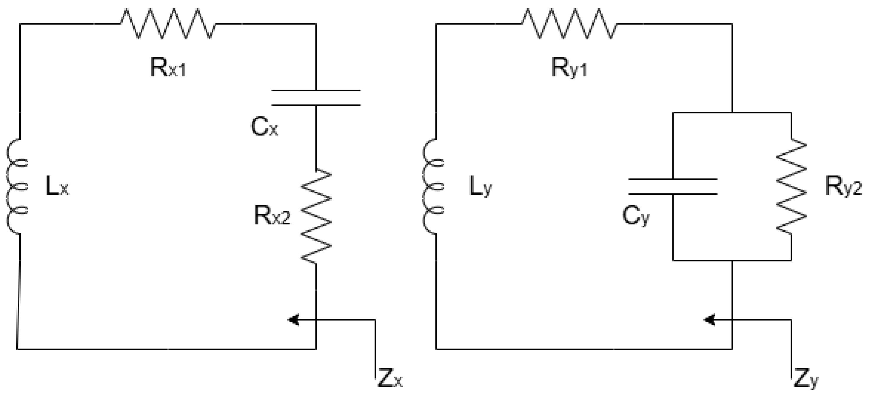
Comparison Between WPT Secondary Circuit with RC Series and RC Parallel

As we stated earlier in our single-capacitor proposed design, a capacitance characteristic is guaranteed to exist in the secondary WPT circuit for battery charging purposes due to the presence of the rectifier circuit. Here, a capacitance characteristic refers to the capacitor $C_L$ in the RC parallel representing the rectifier circuit as the load (see Figure 6). In this part, we compare two different secondary WPT circuits. One is with the RC series that is used in the series-series compensation WPT circuit, and the other is with the RC parallel that we used. Note that this part only serves to provide the comparison between those circuits in a quantitative manner. However, it is not related to the main substance of our proposal.

First, let us focus only on the secondary WPT circuit of two different topologies, as shown in Figure 7, where subscript x refers to the RC series topology, while subscript y refers to the RC parallel topology. In addition, L represents the equivalent inductance of the coils.

Next, the equivalent impedances of both circuits are computed using phasor representation. For the RC series circuit, its equivalent impedance $Z_x$ can be derived as follows:

$$\begin{array}{c}\hfill \begin{array}{cc}\hfill Z_x& =R_{x1}+R_{x2}+i\omega L_x+{\displaystyle \frac{1}{i\omega C_x}}\hfill \\ \hfill Z_x& =\underset{Re\left(Z_x\right)}{\underbrace{R_{x1}+R_{x2}}}+i\underset{Im\left(Z_x\right)}{\underbrace{{\displaystyle \frac{{\omega }^2{L}_x{C}_x-1}{\omega C_x}}}}\hfill \end{array}\end{array}$$

(15)

Meanwhile, for the RC parallel circuit, its equivalent impedance $Z_y$ can be derived as follows:

$$\begin{array}{c}\hfill \begin{array}{cc}\hfill Z_y& =R_{y1}+i\omega L_y+{\displaystyle \frac{1}{i\omega C_y}}\left|\right|R_{y2}\hfill \\ & =R_{y1}+i\omega L_y+{\displaystyle \frac{R_{y2}\frac{1}{i\omega C_y}}{R_{y2}+\frac{1}{i\omega C_y}}}\hfill \\ & =R_{y1}+i\omega L_y+{\displaystyle \frac{R_{y2}}{1+i\omega R_{y2}{C}_y}}\hfill \\ & =R_{y1}+i\omega L_y+{\displaystyle \frac{R_{y2}}{\sqrt{{\omega }^2{R}_{y2}^2{C}_y^2+1}}}\angle ta{n}^{-1}(-\omega R_{y2}{C}_y)\hfill \\ & =R_{y1}+i\omega L_y+{\displaystyle \frac{R_{y2}}{{\omega }^2{R}_{y2}^2{C}_y^2+1}}-i{\displaystyle \frac{\omega R_{y2}^2{C}_y}{{\omega }^2{R}_{y2}^2{C}_y^2+1}}\hfill \\ \hfill Z_y& =\underset{Re\left(Z_y\right)}{\underbrace{R_{y1}+{\displaystyle \frac{R_{y2}}{{\omega }^2{R}_{y2}^2{C}_y^2+1}}}}+i\underset{Im\left(Z_y\right)}{\underbrace{\left(\omega L_y-{\displaystyle \frac{\omega R_{y2}^2{C}_y}{{\omega }^2{R}_{y2}^2{C}_y^2+1}}\right)}}\hfill \end{array}\end{array}$$

(16)

Thus, even though both WPT secondary circuits are similar in terms of the existence of a capacitor, the difference in the topology leads to a distinction in equivalent impedance, as shown in Equations (15) and (16). Furthermore, with the same component parameter values, the resonance frequencies of both circuits are also different.

6. Case Study

6.1. Simulation Parameters Setup

To verify our proposed method, a study case was conducted using MATLAB simulation.

First, a mathematical model of the system as in Figure 6 was built based on Equation (12) by using two different parameter values. The first parameter value is defined in

Table 1. WPT simulation parameter value 1.

${\mathit{R}}_{\mathit{s}}\left(\mathbf{\Omega }\right)$	${\mathit{R}}_1\left(\mathbf{\Omega }\right)$	${\mathit{L}}_1(\mathbf{\mu }$H)	${\mathit{R}}_2\left(\mathbf{\Omega }\right)$	${\mathit{L}}_2(\mathbf{\mu }$H)
1	1	63.4	1	63.4

:

Then, by using the previous parameter value 1 in Table 1 and based on Equations (12) and (14), a frequency response for the system’s power output P with varying coupling coefficient K was plotted by setting the primary capacitance $C=1\mu$F, the load resistance $R_L$ = 10 $\Omega$, the load capacitance $C_L=1\mu$F, and the AC voltage source maximum amplitude normalized as $A_m=1$ to find the highest possible power output. Here, K was chosen as the free variable because it reflects the power transfer distance between the primary and secondary coils to which the WPT system is very sensitive [10]. Since $0<K<1$, the range of K values in the simulation was set to [0.1:0.1:0.9] to represent every possibility while lowering the computational cost. The frequency response for the parameter value 1 is shown in Figure 8. It is seen that the highest power output value for different K is $P=0.0952$ W.

For the second parameter value, the difference is only on both coil inductances $L_1$ and $L_2$, as seen in

Table 2. WPT simulation parameter value 2.

${\mathit{R}}_{\mathit{s}}\left(\mathbf{\Omega }\right)$	${\mathit{R}}_1\left(\mathbf{\Omega }\right)$	${\mathit{L}}_1(\mathbf{\mu }$H)	${\mathit{R}}_2\left(\mathbf{\Omega }\right)$	${\mathit{L}}_2(\mathbf{\mu }$H)
1	1	40	1	40

:

Then, with the same values of C, $R_L$, $C_L$, and $A_m$ as before, the frequency response of the system’s power output P with varying K was plotted, which is shown in Figure 9.

Once again, we can see that the highest power output with parameter value 2 is around P = 0.0881 W.

Then, two scenarios were investigated using a specific GA setup. In the first scenario, the coupling coefficient K was varied while the load parameter values $C_L$ and $R_L$ were fixed. In contrast, in the second scenario, $C_L$ and $R_L$ were varied while K was fixed. Here, both scenarios’ objective is to observe whether the optimization parameter by GA can achieve the possible highest power delivery described in the system frequency response seen in Figure 8 and Figure 9. Finally, in the third scenario, the effect of some variances in the GA’s population sizes, crossover fraction, and different set of initial populations on the highest power delivery result was computed based on the system parameter value 2. This scenario is a sensitivity analysis to investigate the consistency or the convergence of the GA in fulfilling the objective function subject to the same constraints.

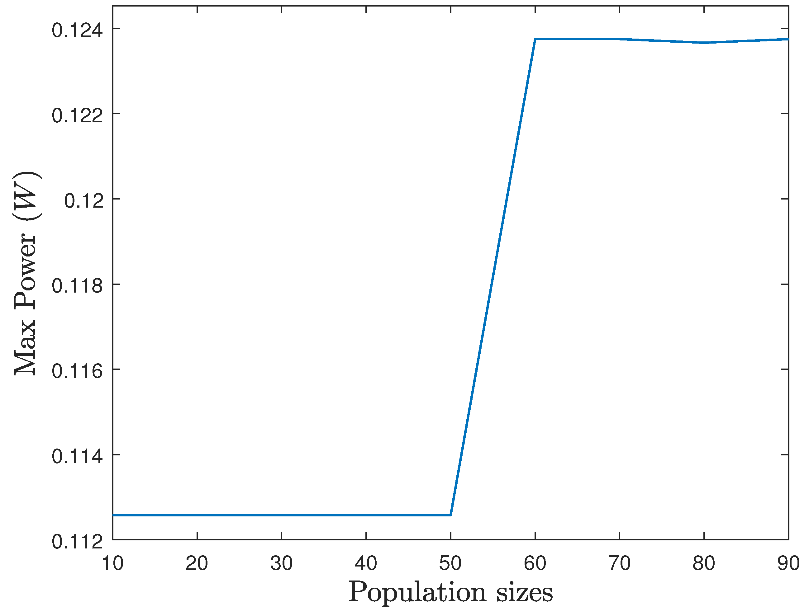
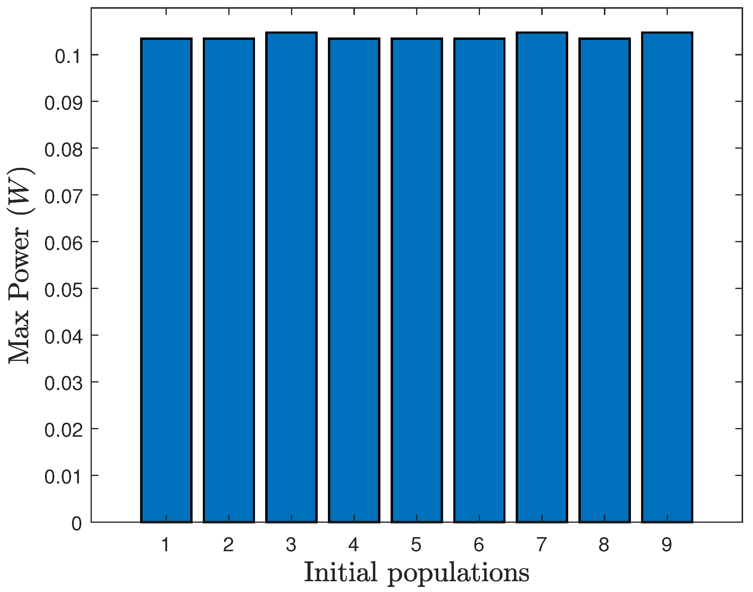
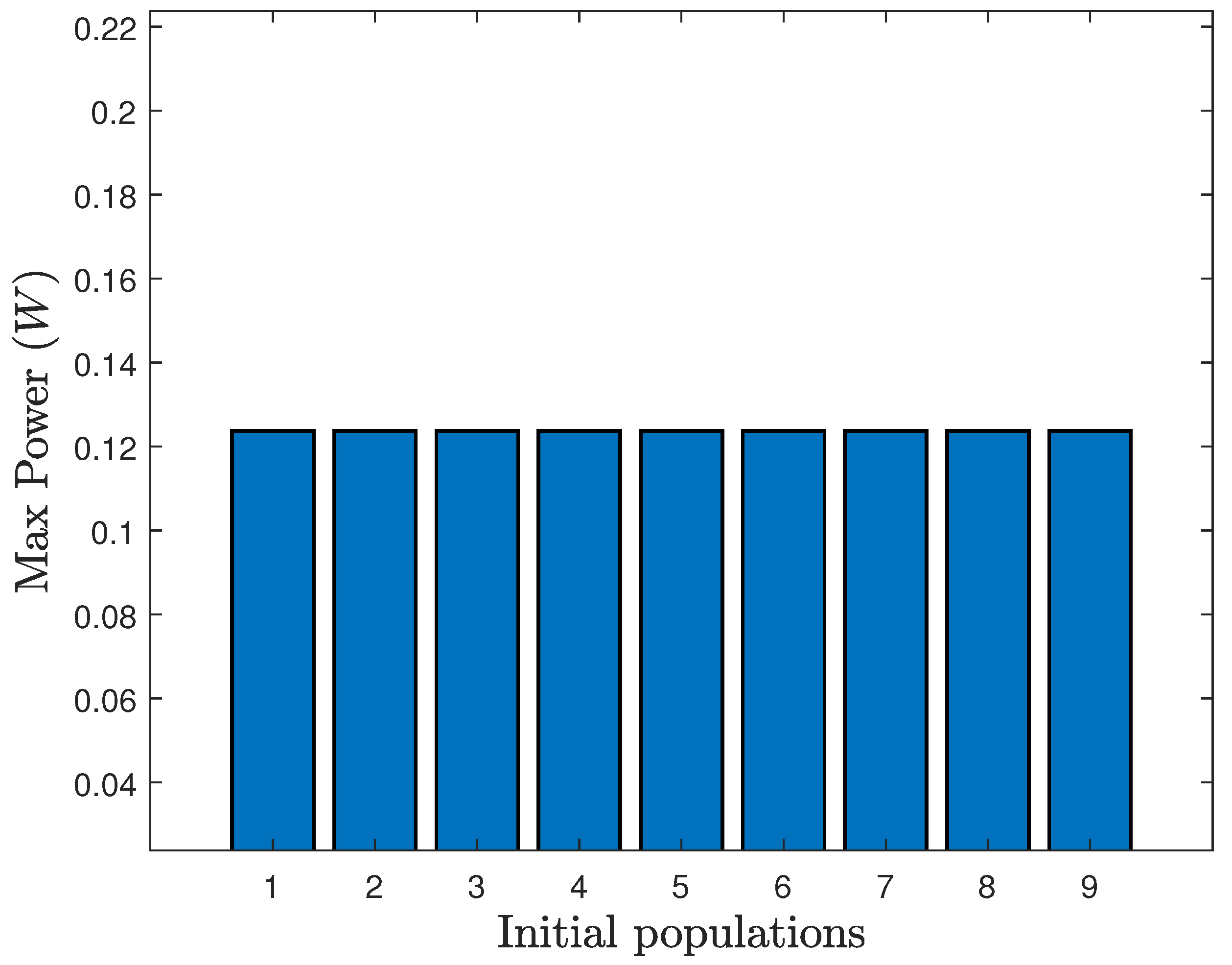
6.2. GA Implementation Setup

For the first and second scenarios, the optimum values of primary capacitance C and voltage source frequency f were searched to achieve the highest power P. To find them, we chose to use a heuristic method by using a MATLAB built-in GA toolbox. By still normalizing $A_m=1$, Equation (14) was chosen as the GA fitness function, while the only constraints were the lower and upper bound values of C and f.

In detail, the GA settings used in MATLAB were as follows:

• Population size: 60;
• Max generations: 600;
• Function tolerance: ${10}^{-6}$;
• Lower bounds for primary capacitance C: ${10}^{-12}$ F;
• Upper bounds for primary capacitance C: ${10}^{-3}$ F;
• Lower bounds for frequency source f: ${10}^3$ Hz;
• Upper bounds for frequency source f: ${10}^6$ Hz;
• Initial population range: lower bounds and upper bounds for C and f;
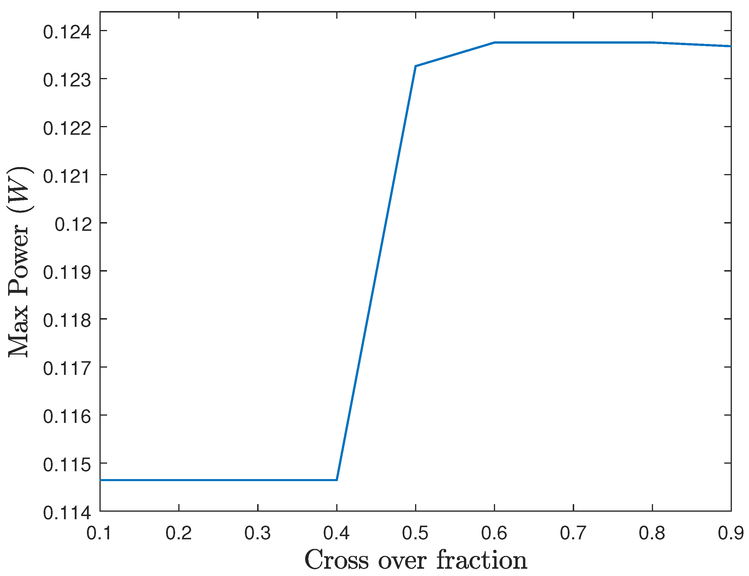
• Crossover fraction: $0.5$;
• Crossover function: @crossoverintermediate, 15;
• Mutation function: @mutationadaptfeasible, $0.01$, 20.

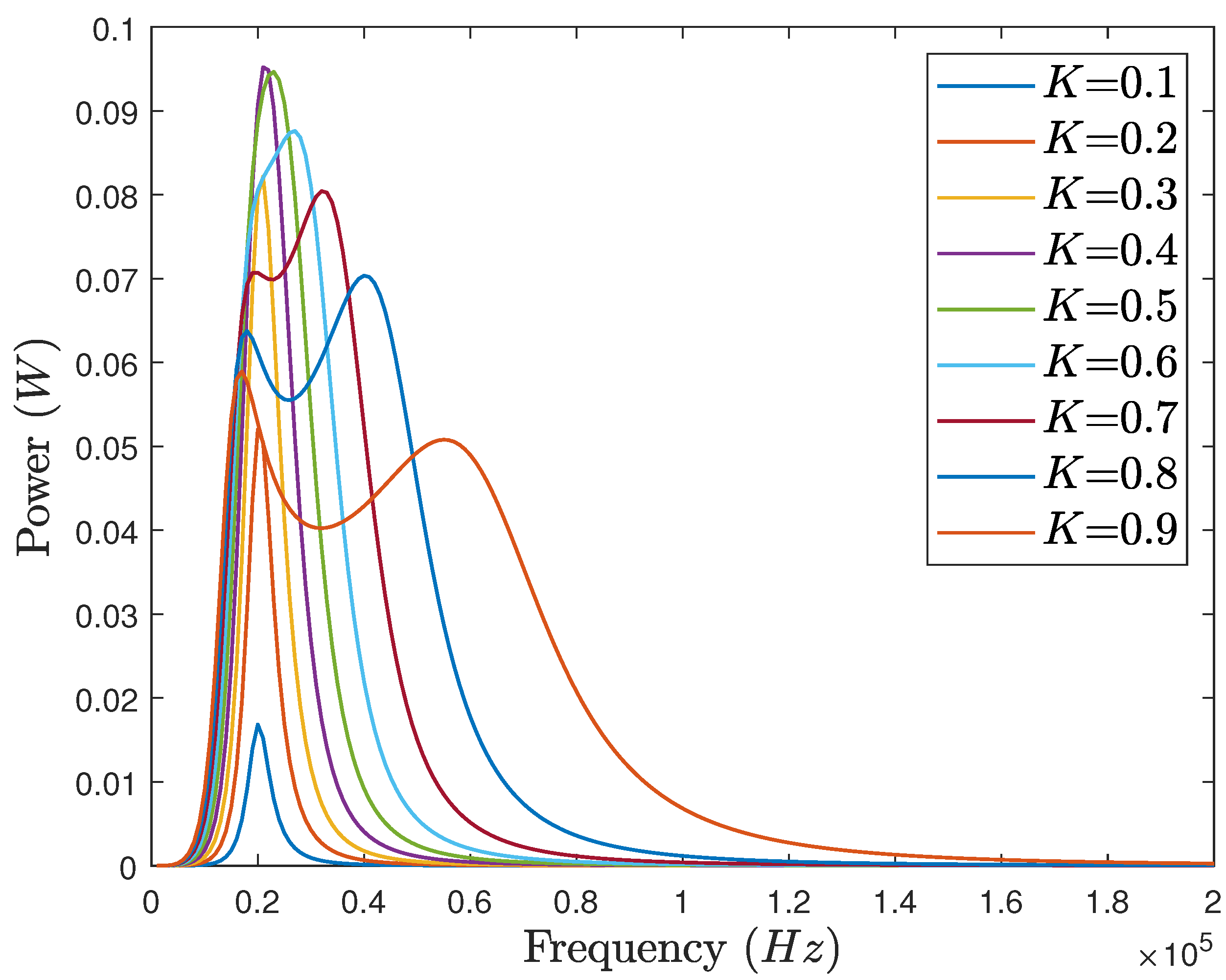
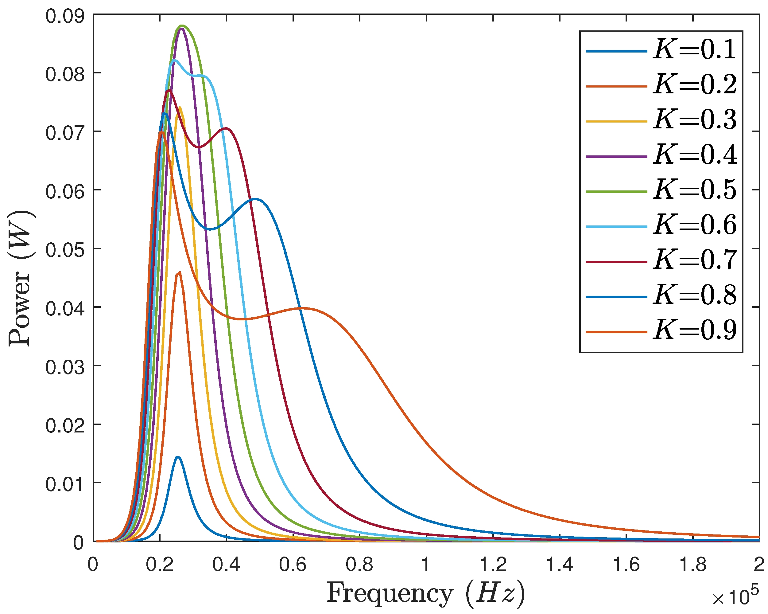
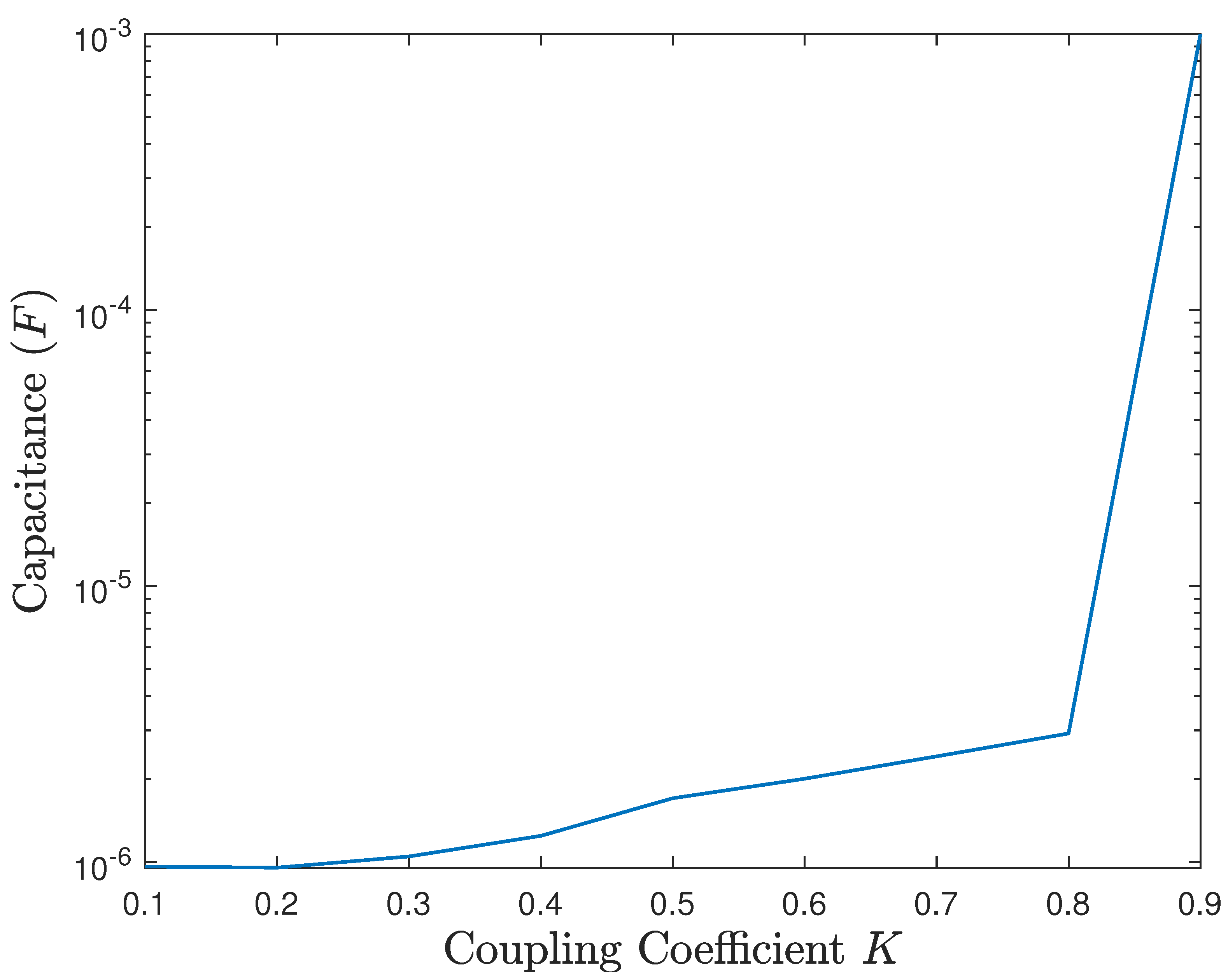
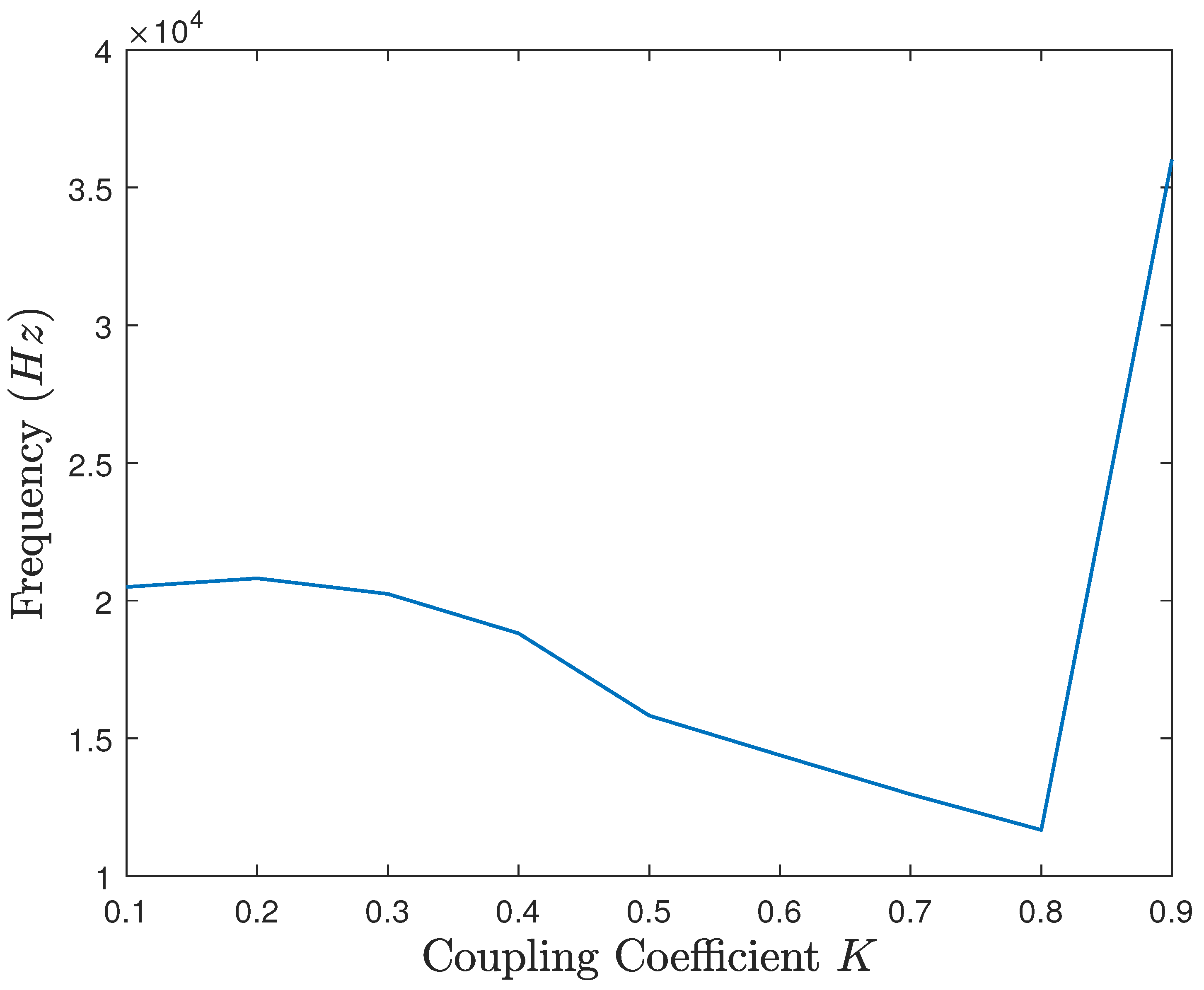
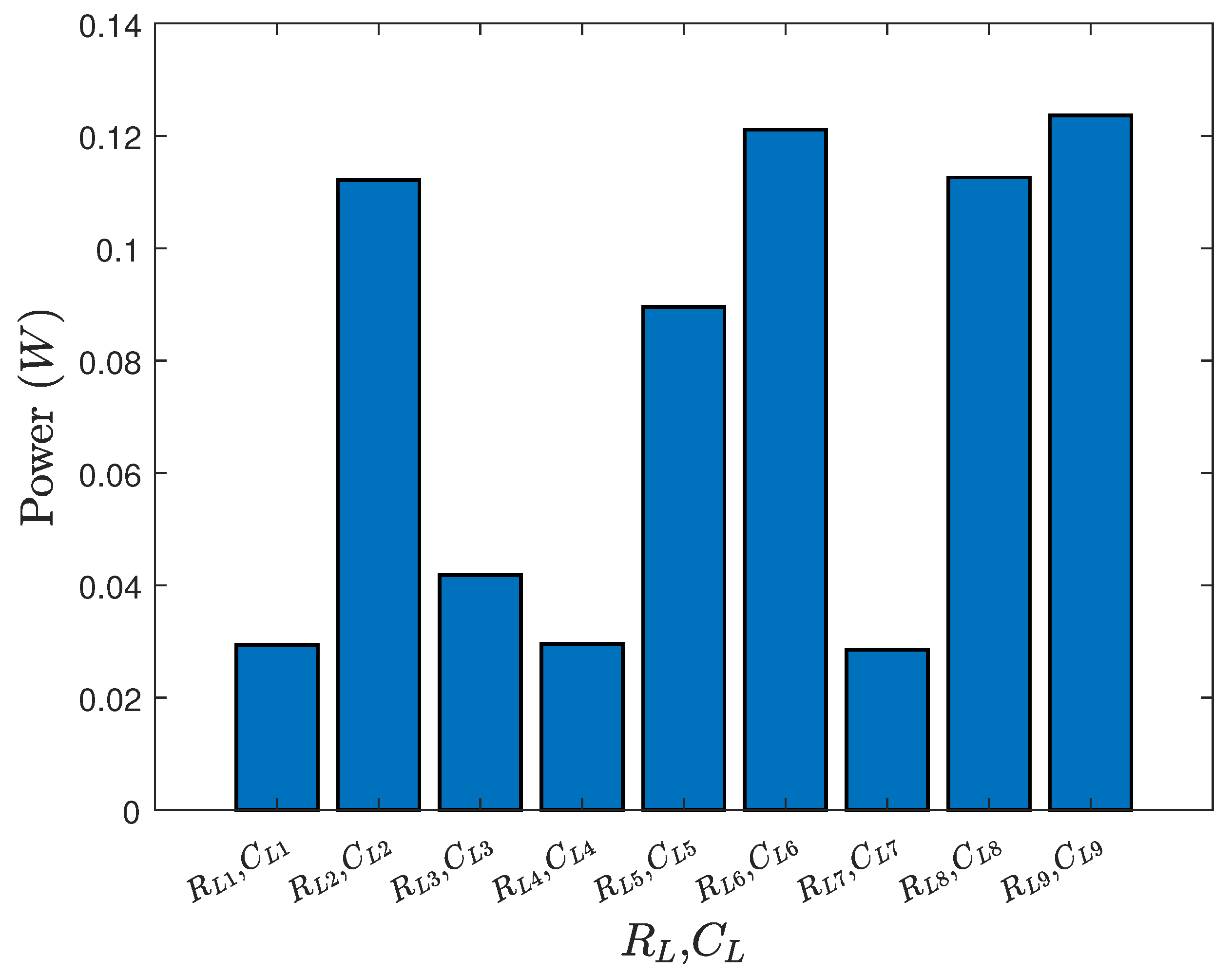
6.3. Simulation Results

For the first scenario, the parameter value 1 defined in Table 1 was used along with the load parameter values, which were made constant as $R_L=10\Omega$ and $C_L=1\mu$F, while the various coupling coefficients K values were [0.1:0.1:0.9]. Using the GA, the solutions of C and f are shown in Figure 10 and Figure 11, respectively. Meanwhile, the power output P related to the previous C and f solutions is shown in Figure 12. It is seen there that the highest power output is $P=0.1082$ W.

Then, the same simulation to find the optimum C, f, and their related P values was run again but with parameter value 2 defined in Table 2. In this case, the solutions of C and f are shown in Figure 13 and Figure 14, respectively. Meanwhile, the power output P is shown in Figure 15. It is seen there that the highest power output is $P=0.1034$ W.

For the second scenario, the coupling coefficient value K was taken constant as $K=0.4$ with parameter value 1 as defined in Table 1. Meanwhile, the various ith combination values of $R_{Li}$ and $C_{Li}$ in the load were taken as defined in

Table 3. Load simulation parameter values.

i	1	2	3	4	5	6	7	8	9
$R_{Li}(\Omega )$	1	10	100	1	10	100	1	10	100
$C_{Li}\left(F\right)$	${10}^{-12}$	${10}^{-9}$	${10}^{-6}$	${10}^{-9}$	${10}^{-6}$	${10}^{-12}$	${10}^{-6}$	${10}^{-12}$	${10}^{-9}$

, where i represents the ith combination values of $R_{Li}$ and $C_{Li}$.

Again, by using the GA, the solutions of C and f are shown in Figure 16 and Figure 17, respectively. Meanwhile, the power output P related to the previous C and f solutions is shown in Figure 18. It is seen there that the highest power output is P = 0.1238 W.

Then, the same simulation was run again but by using parameter value 2 as defined in Table 2. In this case, the solutions of C and f are shown in Figure 19 and Figure 20, respectively. Meanwhile, the power output P is shown in Figure 21. It is seen that the highest power output is P = 0.1236 W.

Finally, in this third scenario, a variance of [10:10:90] in the GA population size, a variance of [0.1:0.1:0.9] in the GA crossover fraction, and nine different sets of randomized initial populations were applied in optimizing C and f for the system with the parameter value 2. Figure 22 and Figure 23 show the achieved maximum power P under varying K and varying combinations of $R_L$ and $C_L$, respectively, with varying population sizes, while the other parameters were the same as the previous GA setup seen in Section 6.2. It is seen there that the population size of 60 was good enough to keep the consistent results.

Meanwhile, for varying crossover fractions, Figure 24 and Figure 25 show the achieved maximum power P under varying K and varying combinations of $R_L$ and $C_L$, respectively, while the other parameters were the same as the previous GA setup in Section 6.2. It is seen there that the crossover fraction of $0.5$ was good enough to keep the consistent results.

Then, for the varying set of randomized initial populations, Figure 26 and Figure 27 display the achieved maximum power P under varying K and varying combinations of $R_L$ and $C_L$, respectively, while the other parameters were the same as the previous GA setup in Section 6.2. It is seen there that the maximum achieved power disparity is very small, almost unnoticeable, even under nine different set of randomized initial populations.

6.4. Discussion

From the simulation results of the first two scenarios with two different system parameter values, almost the same characteristic related to the highest power output P was observed, even though the optimum C and f solutions varied.

For the system parameter value 1 displayed in Table 1, the frequency response with varying K in Figure 8 shows that frequency splitting occurred as K increased beyond the critical point. For details on the critical point, see [49]. In this regime, the highest observed power output was P = 0.0953 W. Then, using the GA to optimize C and f, the obtained highest power output values came out to $P=0.1082$ W for varying K in Figure 12 and P = 0.1238 W for varying load in Figure 18, which show similar or higher values than the system frequency response.

Similarly, with the system parameter value 2 displayed in Table 2, the frequency response with varying K in Figure 9 demonstrates that frequency splitting was present, with the highest observed power output reaching $P=0.0881$ W. Then, using the GA to optimize C and f, the obtained highest power output values came out to P = 0.1034 W for varying K in Figure 15 and P = 0.1236 W for varying load in Figure 21, which show similar or higher values than the system frequency response.

Meanwhile, for GA sensitivity analysis, the highest power delivery for the system parameter value 2 subjected to a variation in the population sizes with varying K shown in Figure 22 and with varying combinations of load parameters $R_L$ and $C_L$ shown in Figure 23 displays a consistent result, with only a small P difference of less than ${10}^{-2}$ W. The same characteristic was also seen with a varying K and varying combinations of $R_L$ and $C_L$ subjected to a variation in GA crossover fractions, as shown in Figure 24 and Figure 25, respectively. Furthermore, with a varying K and varying combinations of $R_L$ and $C_L$ subjected to different sets of randomized initial populations shown in Figure 26 and Figure 27, respectively, the variation in maximum achieved power delivery is almost unnoticeable. Thus, the GA settings used in the simulation are reliable enough to guarantee the convergence of the optimization results.

Note that the small values of P are because the AC voltage source maximum amplitude was normalized to 1 ($A_m=1$). If it is increased, then P will also increase proportional to the $A_m^2$; see Equation (14).

Hence, it can be concluded that a single-capacitor WPT can be optimized by varying the primary capacitance value C and voltage source frequency f, using the GA, to achieve high power output P to the load, which represents a full bridge rectifier. The single capacitor is put on the WPT transmitter side so that the optimization can be designed regardless of the load. This approach is simpler in complexity compared to other existing compensation methods.

However, since this study is theoretical research, more work needs to be done to achieve the end goal of a single-capacitor WPT approach to charge batteries. First, the simplification of a full bridge rectifier into an RC parallel is only valid on small AC signal analysis. In our study, this simplification was chosen because we are interested in the structure of the linear relation between the WPT voltage source and the rectifier voltage output so that we can choose reasonable optimization parameters and also decide on what method to solve the optimization problem. The related relationship is seen in Equations (12)–(14). By observing those equations, it can be concluded that using function derivation to find the zero solution in finding the optimum values is hard. Still, by defining the power delivery as an objective function and the available optimization parameter values, it is easier to put them into the GA to find the solution. Second, this study lacks a power transfer efficiency analysis. Third, as the verification of the proposed method is only via a simulation process, a hardware experiment is necessary for future works. Thus, along with that experiment, a further investigation regarding power transfer efficiency can also be addressed. Finally, the GA sensitivity analysis can also be extended to include variations in the number of generations, function tolerance, crossover and mutation functions, etc. It is also possible to investigate other optimization methods besides the GA.

7. Conclusions

In this study, a preliminary theoretical investigation has been conducted for a WPT system to charge mobile device batteries. In contrast to other proposed approaches that tend to add components or circuits so that the overall system becomes more complex, the design of a single capacitor on the WPT transmitter side is proposed here. This single-capacitor approach is due to the fact that a capacitance characteristic always exists on the receiver side because of the presence of the rectifier circuit.

Since the WPT output needs to be rectified to charge batteries, a full bridge rectifier circuit is used to represent the WPT load. The mathematical models for the rectifier and the single-capacitor WPT are then built and combined by utilizing state space and transfer function methods. After that, based on the model, an optimization process using GA can be used to find the optimum solutions to achieve the highest power output.

By setting the capacitance value in the primary side and the AC voltage source frequency as the tunable parameters, the simulation results showed that the optimum solutions by the GA could be obtained for producing the highest power transfer of a single-capacitor WPT design despite its asymmetry and inability to facilitate resonance. Moreover, the results are consistent with the system’s frequency response.

Since the study focused on high power delivery, further work in examining the efficiency of power transfer and investigating the hardware implementation is planned to be done. Related to the optimization using the GA, since this study examined the convergences only by changing one GA hyperparameter per action, an extended GA sensitivity analysis by simultaneously changing more than one hyperparameter is worth investigating. Furthermore, the possibility of other methods for optimization purposes can also be considered in future works.

References

1. Hong, Y.W.P.; Hsu, T.C.; Chennakesavula, P. Wireless power transfer for distributed estimation in wireless passive sensor networks. IEEE Trans. Signal Process. 2016, 64, 5382–5395. [Google Scholar] [CrossRef]
2. Shan, D.; Wang, H.; Cao, K.; Zhang, J. Wireless power transfer system with enhanced efficiency by using frequency reconfigurable metamaterial. Sci. Rep. 2022, 12, 331. [Google Scholar]
3. Gore, V.B.; Gawali, D.H. Wireless power transfer technology for medical applications. In Proceedings of the 2016 Conference on Advances in Signal Processing (CASP), Pune, India, 9–11 June 2016; pp. 455–460. [Google Scholar]
4. Joseph, P.K.; Elangovan, D. A review on renewable energy powered wireless power transmission techniques for light electric vehicle charging applications. J. Energy Storage 2018, 16, 145–155. [Google Scholar]
5. Chan, C.C.; Chau, K. An overview of power electronics in electric vehicles. IEEE Trans. Ind. Electron. 1997, 44, 3–13. [Google Scholar]
6. Barsukov, Y.; Qian, J. Battery Power Management for Portable Devices; Artech House: Norwood, MA, USA, 2013. [Google Scholar]
7. Abdul-Jabbar, T.A.; Obed, A.A.; Abid, A.J. Design of an uninterrupted power supply with Li-ion battery pack: A proposal for a cost-efficient design with high protection features. J. Tech. 2021, 3, 1–10. [Google Scholar]
8. Hui, S. Wireless power transfer: A brief review & update. In Proceedings of the 2013 5th International Conference on Power Electronics Systems and Applications (PESA), Hong Kong, China, 11–13 December 2013; pp. 1–4. [Google Scholar]
9. Rim, C.T.; Mi, C. Wireless Power Transfer for Electric Vehicles and Mobile Devices; John Wiley & Sons: Hoboken, NJ, USA, 2017. [Google Scholar]
10. Zhang, Z.; Pang, H.; Georgiadis, A.; Cecati, C. Wireless power transfer—An overview. IEEE Trans. Ind. Electron. 2018, 66, 1044–1058. [Google Scholar]
11. Brecher, A.; Arthur, D. Review and evaluation of wireless power transfer (WPT) for electric transit applications. Repos. Open Sci. Access Portal 2014. Available online: https://rosap.ntl.bts.gov/view/dot/27847/dot_27847_DS1.pdf (accessed on 10 January 2025).
12. Tang, X.; Zeng, J.; Pun, K.P.; Mai, S.; Zhang, C.; Wang, Z. Low-cost maximum efficiency tracking method for wireless power transfer systems. IEEE Trans. Power Electron. 2017, 33, 5317–5329. [Google Scholar]
13. Jawad, A.M.; Nordin, R.; Gharghan, S.K.; Jawad, H.M.; Ismail, M. Opportunities and challenges for near-field wireless power transfer: A review. Energies 2017, 10, 1022. [Google Scholar] [CrossRef]
14. Joseph, B.; Bhoir, D. Design and simulation of wireless power transfer for electric vehicle. In Proceedings of the 2019 International Conference on Advances in Computing, Communication and Control (ICAC3), Mumbai, India, 20–21 December 2019; pp. 1–5. [Google Scholar]
15. Gonda, T.; Mototani, S.; Doki, K.; Torii, A. Effect of air space in waterproof sealed case containing transmitter and receiver of wireless power transfer in sea water. Electr. Eng. Jpn. 2019, 206, 24–31. [Google Scholar]
16. Li, F.; Sun, X.; Zhou, S.; Chen, Y.; Hao, Z.; Yang, Z. Infrastructure material magnetization impact assessment of wireless power transfer pavement based on resonant inductive coupling. IEEE Trans. Intell. Transp. Syst. 2021, 23, 22400–22408. [Google Scholar] [CrossRef]
17. Allam, A.; Patel, H.; Sugino, C.; John, C.S.; Steinfeldt, J.; Reinke, C.; Erturk, A.; El-Kady, I. Portable through-metal ultrasonic power transfer using a dry-coupled detachable transmitter. Ultrasonics 2024, 141, 107339. [Google Scholar] [PubMed]
18. Liu, W.; Chau, K.; Lee, C.H.; Jiang, C.; Han, W.; Lam, W. Multi-frequency multi-power one-to-many wireless power transfer system. IEEE Trans. Magn. 2019, 55, 8001609. [Google Scholar]
19. Qiu, C.; Chau, K.; Liu, C.; Chan, C.C. Overview of wireless power transfer for electric vehicle charging. In Proceedings of the 2013 World Electric Vehicle Symposium and Exhibition (EVS27), Barcelona, Spain, 17–20 November 2013; pp. 1–9. [Google Scholar]
20. Li, S.; Mi, C.C. Wireless power transfer for electric vehicle applications. IEEE J. Emerg. Sel. Top. Power Electron. 2014, 3, 4–17. [Google Scholar]
21. Moore, J.; Castellanos, S.; Xu, S.; Wood, B.; Ren, H.; Tse, Z.T.H. Applications of wireless power transfer in medicine: State-of-the-art reviews. Ann. Biomed. Eng. 2019, 47, 22–38. [Google Scholar]
22. Yoo, S.; Lee, J.; Joo, H.; Sunwoo, S.H.; Kim, S.; Kim, D.H. Wireless power transfer and telemetry for implantable bioelectronics. Adv. Healthc. Mater. 2021, 10, 2100614. [Google Scholar]
23. Askari, A.; Stark, R.; Curran, J.; Rule, D.; Lin, K. Underwater wireless power transfer. In Proceedings of the 2015 IEEE Wireless Power Transfer Conference (WPTC), Boulder, CO, USA, 13–15 May 2015; pp. 1–4. [Google Scholar]
24. Mohsan, S.A.H.; Islam, A.; Khan, M.A.; Mahmood, A.; Rokia, L.S.; Mazinani, A.; Amjad, H. A review on research challenges limitations and practical solutions for underwater wireless power transfer. Int. J. Adv. Comput. Sci. Appl. 2020, 11, 554–562. [Google Scholar]
25. Zhang, B.; Xu, W.; Lu, C.; Lu, Y.; Wang, X. Review of low-loss wireless power transfer methods for autonomous underwater vehicles. IET Power Electron. 2022, 15, 775–788. [Google Scholar]
26. Okoyeigbo, O.; Olajube, A.; Shobayo, O.; Aligbe, A.; Ibhaze, A. Wireless power transfer: A review. In Proceedings of the IOP Conference Series: Earth and Environmental Science; IOP Publishing: Bristol, UK, 2021; Volume 655, p. 012032. [Google Scholar]
27. Malik, H.; Ahmad, M.W.; Kothari, D.P. Intelligent Data Analytics for Power and Energy Systems; Springer: Berlin/Heidelberg, Germany, 2022; Volume 802. [Google Scholar]
28. Kurs, A.; Karalis, A.; Moffatt, R.; Joannopoulos, J.D.; Fisher, P.; Soljacic, M. Wireless power transfer via strongly coupled magnetic resonances. Science 2007, 317, 83–86. [Google Scholar]
29. Summerer, L.; Purcell, O. Concepts for Wireless Energy Transmission via Laser; Europeans Space Agency (ESA)-Advanced Concepts Team: 2009. Available online: https://www.academia.edu/download/69382807/Paper_69-A_Review_on_Research_Challenges.pdf (accessed on 10 January 2025).
30. Yeoh, W. Wireless Power Transmission (WPT) Application at 2.4 GHz in Common Network. Ph.D. Thesis, RMIT University, Melbourne, Australia, 2010. [Google Scholar]
31. Li, J.L.W. Wireless power transmission: State-of-the-arts in technologies and potential applications. In Proceedings of the Asia-Pacific Microwave Conference 2011, Melbourne, Australia, 5–8 December 2011; pp. 86–89. [Google Scholar]
32. Tomar, A.; Gupta, S. Wireless power transmission: Applications and components. Int. J. Eng. 2012, 1, 1–8. [Google Scholar]
33. Kumar, S.; Singh, S.K.; Mehta, S.K.; Singh, R.K.; Kumar, S.; Dangi, R.S.P. Wireless power transmission-a prospective idea for future. IRNet Undergrad. Acad. Res. J. 2012. [Google Scholar]
34. Popovic, Z. Near-and far-field wireless power transfer. In Proceedings of the 2017 13th International Conference on Advanced Technologies, Systems and Services in Telecommunications (TELSIKS), Niš, Serbia, 18–20 October 2017; pp. 3–6. [Google Scholar]
35. Zhang, H.; Shlezinger, N.; Guidi, F.; Dardari, D.; Imani, M.F.; Eldar, Y.C. Near-field wireless power transfer for 6G internet of everything mobile networks: Opportunities and challenges. IEEE Commun. Mag. 2022, 60, 12–18. [Google Scholar]
36. Covic, G.A.; Boys, J.T. Inductive power transfer. Proc. IEEE 2013, 101, 1276–1289. [Google Scholar]
37. Mayordomo, I.; Dräger, T.; Spies, P.; Bernhard, J.; Pflaum, A. An overview of technical challenges and advances of inductive wireless power transmission. Proc. IEEE 2013, 101, 1302–1311. [Google Scholar]
38. Mahmood, A.; Ismail, A.; Zaman, Z.; Fakhar, H.; Najam, Z.; Hasan, M.; Ahmed, S. A comparative study of wireless power transmission techniques. J. Basic Appl. Sci. Res. 2014, 4, 321–326. [Google Scholar]
39. Liu, C.; Hu, A.P. Steady state analysis of a capacitively coupled contactless power transfer system. In Proceedings of the 2009 IEEE Energy Conversion Congress and Exposition, San Jose, CA, USA, 20–24 September 2009; pp. 3233–3238. [Google Scholar]
40. Liu, C.; Hu, A.P.; Nair, N.K. Modelling and analysis of a capacitively coupled contactless power transfer system. IET Power Electron. 2011, 4, 808–815. [Google Scholar]
41. El Rayes, M.M.; Nagib, G.; Abdelaal, W.A. A review on wireless power transfer. Int. J. Eng. Trends Technol. (IJETT) 2016, 40, 272–280. [Google Scholar]
42. Detka, K.; Górecki, K. Wireless power transfer—A review. Energies 2022, 15, 7236. [Google Scholar] [CrossRef]
43. Kim, D.; Abu-Siada, A.; Sutinjo, A. State-of-the-art literature review of WPT: Current limitations and solutions on IPT. Electr. Power Syst. Res. 2018, 154, 493–502. [Google Scholar]
44. Sidiku, M.; Eronu, E.; Ashigwuike, E. A review on wireless power transfer: Concepts, implementations, challenges, and mitigation scheme. Niger. J. Technol. 2020, 39, 1206–1215. [Google Scholar]
45. Soni, S.; Gupta, S. WPT Techniques based Power Transmission: A State-of-Art Review. In Proceedings of the 2022 13th International Conference on Computing Communication and Networking Technologies (ICCCNT), Virtual, 3–5 October 2022; pp. 1–6. [Google Scholar]
46. Sohn, Y.H.; Choi, B.H.; Lee, E.S.; Lim, G.C.; Cho, G.H.; Rim, C.T. General unified analyses of two-capacitor inductive power transfer systems: Equivalence of current-source SS and SP compensations. IEEE Trans. Power Electron. 2015, 30, 6030–6045. [Google Scholar] [CrossRef]
47. Lau, K. Comparative Study of Different Coil Geometries for Wireless Power Transfer. In Proceedings of the Final Dissertation (Final)—Lau Kevin 16392. IRC, 2016. Available online: http://utpedia.utp.edu.my/id/eprint/17133/ (accessed on 10 January 2025).
48. Pahlavan, S.; Shooshtari, M.; Jafarabadi Ashtiani, S. Star-Shaped Coils in the Transmitter Array for Receiver Rotation Tolerance in Free-Moving Wireless Power Transfer Applications. Energies 2022, 15, 8643. [Google Scholar] [CrossRef]
49. Niu, S.; Lyu, R.; Lyu, J.; Chau, K.; Liu, W.; Jian, L. Optimal resonant condition for maximum output power in tightly-coupled WPT systems considering harmonics. IEEE Trans. Power Electron. 2024, 40, 152–156. [Google Scholar] [CrossRef]
50. Niu, S.; Yu, H.; Niu, S.; Jian, L. Power loss analysis and thermal assessment on wireless electric vehicle charging technology: The over-temperature risk of ground assembly needs attention. Appl. Energy 2020, 275, 115344. [Google Scholar] [CrossRef]
51. Niu, S.; Zhao, Q.; Chen, H.; Niu, S.; Jian, L. Noncooperative metal object detection using pole-to-pole EM distribution characteristics for wireless EV charger employing DD coils. IEEE Trans. Ind. Electron. 2023, 71, 6335–6344. [Google Scholar] [CrossRef]
52. Akbar, S.R.; Setiawan, E.; Hirata, T.; Hodaka, I. Optimal Wireless Power Transfer Circuit without a Capacitor on the Secondary Side. Energies 2023, 16, 2922. [Google Scholar] [CrossRef]
53. Song, K.; Lan, Y.; Zhang, X.; Jiang, J.; Sun, C.; Yang, G.; Yang, F.; Lan, H. A review on interoperability of wireless charging systems for electric vehicles. Energies 2023, 16, 1653. [Google Scholar] [CrossRef]
54. Thongpron, J.; Kamnarn, U.; Namin, A.; Sriprom, T.; Chaidee, E.; Janjornmanit, S.; Yachiangkam, S.; Karnjanapiboon, C.; Thounthong, P.; Takorabet, N. Varied-Frequency CC–CV Inductive Wireless Power Transfer with Efficiency-Regulated EV Charging for an Electric Golf Cart. Energies 2023, 16, 7388. [Google Scholar] [CrossRef]
55. Pagano, R.; Abedinpour, S.; Raciti, A.; Musumeci, S. Efficiency optimization of an integrated wireless power transfer system by a genetic algorithm. In Proceedings of the 2016 IEEE Applied Power Electronics Conference and Exposition (APEC), Long Beach, CA, USA, 20–24 March 2016; pp. 3669–3676. [Google Scholar]
56. Gao, X.; Cao, W.; Yang, Q.; Wang, H.; Wang, X.; Jin, G.; Zhang, J. Parameter optimization of control system design for uncertain wireless power transfer systems using modified genetic algorithm. CAAI Trans. Intell. Technol. 2022, 7, 582–593. [Google Scholar] [CrossRef]
57. Bertolini, V.; Corti, F.; Intravaia, M.; Reatti, A.; Cardelli, E. Optimizing power transfer in selective wireless charging systems: A genetic algorithm-based approach. J. Magn. Magn. Mater. 2023, 587, 171340. [Google Scholar] [CrossRef]
58. Patil, D.; McDonough, M.K.; Miller, J.M.; Fahimi, B.; Balsara, P.T. Wireless power transfer for vehicular applications: Overview and challenges. IEEE Trans. Transp. Electrif. 2017, 4, 3–37. [Google Scholar]
59. Liu, W.; Chau, K.; Tian, X.; Wang, H.; Hua, Z. Smart wireless power transfer—opportunities and challenges. Renew. Sustain. Energy Rev. 2023, 180, 113298. [Google Scholar]
60. Yamaguchi, K.; Hirata, T.; Yamamoto, Y.; Hodaka, I. Resonance and efficiency in wireless power transfer system. WSEAS Trans. Circuits Syst. 2014, 13, 218–223. [Google Scholar]
61. Love, G.N.; Wood, A.R. Harmonic state space model of power electronics. In Proceedings of the 2008 13th International Conference on Harmonics and Quality of Power, Wollongong, NSW, Australia, 28 September–1 October 2008; pp. 1–6. [Google Scholar]
62. Blanchette, H.F.; Ould-Bachir, T.; David, J.P. A state-space modeling approach for the FPGA-based real-time simulation of high switching frequency power converters. IEEE Trans. Ind. Electron. 2011, 59, 4555–4567. [Google Scholar] [CrossRef]
63. Emadi, A. Modeling and analysis of multiconverter DC power electronic systems using the generalized state-space averaging method. IEEE Trans. Ind. Electron. 2004, 51, 661–668. [Google Scholar]
64. Erickson, R.W.; Maksimovic, D. Fundamentals of Power Electronics; Springer Science & Business Media: Berlin/Heidelberg, Germany, 2007. [Google Scholar]
65. Hart, D.W.; Hart, D.W. Power Electronics; McGraw-Hill: New York, NY, USA, 2011; Volume 166. [Google Scholar]
66. Kolar, J.W.; Krismer, F.; Lobsiger, Y.; Muhlethaler, J.; Nussbaumer, T.; Minibock, J. Extreme efficiency power electronics. In Proceedings of the 2012 7th International Conference on Integrated Power Electronics Systems (CIPS), Nuremberg, Germany, 6–8 March 2012; pp. 1–22. [Google Scholar]
67. Cameron, I.T.; Hangos, K. Process Modelling and Model Analysis; Elsevier: Amsterdam, The Netherlands, 2001. [Google Scholar]
68. Hangos, K.M.; Bokor, J.; Szederkényi, G. Analysis and Control of Nonlinear Process Systems; Springer Science & Business Media: Berlin/Heidelberg, Germany, 2006. [Google Scholar]
69. Szederkényi, G.; Lakner, R.; Gerzson, M. Intelligent Control Systems: An Introduction with Examples; Springer Science & Business Media: Berlin/Heidelberg, Germany, 2006; Volume 60. [Google Scholar]
70. Brunton, S.L.; Kutz, J.N. Data-Driven Science and Engineering: Machine Learning, Dynamical Systems, and Control; Cambridge University Press: Cambridge, UK, 2022. [Google Scholar]
71. Callier, F.M.; Desoer, C.A. Linear System Theory; Springer Science & Business Media: Berlin/Heidelberg, Germany, 2012. [Google Scholar]
72. Hespanha, J.P. Linear Systems Theory; Princeton University Press: Princeton, NJ, USA, 2018. [Google Scholar]
73. Ogata, K. Modern Control Engineering; Prentice Hall India: Hoboken, NJ, USA, 2009. [Google Scholar]
74. Doyle, J.C.; Francis, B.A.; Tannenbaum, A.R. Feedback Control Theory; Courier Corporation: Maharashtra, India, 2013. [Google Scholar]
75. Van Wageningen, D.; Staring, T. The Qi wireless power standard. In Proceedings of the 14th International Power Electronics and Motion Control Conference EPE-PEMC 2010, Ohrid, Macedonia, 6–8 September 2010; pp. S15–S25. [Google Scholar]
76. Liu, X. Qi standard wireless power transfer technology development toward spatial freedom. IEEE Circuits Syst. Mag. 2015, 15, 32–39. [Google Scholar]
77. Kiruthiga, G.; Jayant, M.Y.; Sharmila, A. Wireless charging for low power applications using Qi standard. In Proceedings of the 2016 International Conference on Communication and Signal Processing (ICCSP), Melmaruvathur, Tamilnadu, India, 6–8 April 2016; pp. 1180–1184. [Google Scholar]
78. Roman, J.; Sindia, S.; Yao, Z.; Briggs, M.; Barber, C. Wireless Power Transfer (WPT) by Magnetic Induction. In Magnetic Communications: From Theory to Practice; CRC Press: Boca Raton, FL, USA, 2018; pp. 3–16. [Google Scholar]
79. Itoh, K. RF bridge rectifier and its good possibility for wireless power transmission systems. In Proceedings of the 2015 IEEE International Symposium on Radio-Frequency Integration Technology (RFIT), Sendai, Japan, 26–28 August 2015; pp. 226–228. [Google Scholar]
80. Fu, M.; Tang, Z.; Liu, M.; Ma, C.; Zhu, X. Full-bridge rectifier input reactance compensation in megahertz wireless power transfer systems. In Proceedings of the 2015 IEEE PELS Workshop on Emerging Technologies: Wireless Power (2015 WoW), IEEE, Daejeon, Republic of Korea, 5–6 June 2015; pp. 1–5. [Google Scholar]
81. Fu, M.; Tang, Z.; Ma, C. Analysis and optimized design of compensation capacitors for a megahertz WPT system using full-bridge rectifier. IEEE Trans. Ind. Inform. 2018, 15, 95–104. [Google Scholar]
82. Sampath, J.; Alphones, A.; Shimasaki, H. Coil design guidelines for high efficiency of wireless power transfer (WPT). In Proceedings of the 2016 IEEE Region 10 Conference (TENCON), Singapore, 22–26 November 2016; pp. 726–729. [Google Scholar]
83. Li, Y.; Jiang, S.; Liu, X.L.; Li, Q.; Dong, W.H.; Liu, J.M.; Ni, X. Influences of coil radius on effective transfer distance in WPT system. IEEE Access 2019, 7, 125960–125968. [Google Scholar] [CrossRef]
84. Rakhymbay, A.; Bagheri, M.; Lu, M. A simulation study on four different compensation topologies in EV wireless charging. In Proceedings of the 2017 International Conference on Sustainable Energy Engineering and Application (ICSEEA), Jakarta, Indonesia, 23–24 October 2017; pp. 66–73. [Google Scholar]
85. Beh, T.C.; Kato, M.; Imura, T.; Oh, S.; Hori, Y. Automated impedance matching system for robust wireless power transfer via magnetic resonance coupling. IEEE Trans. Ind. Electron. 2012, 60, 3689–3698. [Google Scholar]
86. Frivaldsky, M.; Jaros, V.; Spanik, P.; Pavelek, M. Control system proposal for detection of optimal operational point of series–series compensated wireless power transfer system. Electr. Eng. 2020, 102, 1423–1432. [Google Scholar]
Figure 1. Transfer function system block diagram.
Energies 18 01574 g001
Figure 2. The WPT circuit diagram with load.
Energies 18 01574 g002
Figure 3. Full bridge rectifier circuit.
Energies 18 01574 g003
Figure 4. Full bridge rectifier impedance-equivalent circuit.
Energies 18 01574 g004
Figure 5. RC parallel circuit.
Energies 18 01574 g005
Figure 6. The WPT circuit diagram with RC parallel as load.
Energies 18 01574 g006
Figure 7. The WPT secondary circuit diagram with RC series and RC parallel.
Energies 18 01574 g007
Figure 8. Frequency response of system’s power with parameter value 1.
Energies 18 01574 g008
Figure 9. Frequency response of system’s power with parameter value 2.
Energies 18 01574 g009
Figure 10. Primary capacitance with varying K and fixed combination of R L and C L using parameter value 1.
Energies 18 01574 g010
Figure 11. Frequency source with varying K and fixed combination of R L and C L using parameter value 1.
Energies 18 01574 g011
Figure 12. Power output with varying K and fixed combination of R L and C L using parameter value 1.
Energies 18 01574 g012
Figure 13. Primary capacitance with varying K and fixed combination of R L and C L using parameter value 2.
Energies 18 01574 g013
Figure 14. Frequency source with varying K and fixed combination of R L and C L using parameter value 2.
Energies 18 01574 g014
Figure 15. Power output with varying K and fixed combination of R L and C L using parameter value 2.
Energies 18 01574 g015
Figure 16. Primary capacitance with fixed K and varying combinations of R L and C L using parameter value 1.
Energies 18 01574 g016
Figure 17. Frequency source with fixed K and varying combinations of R L and C L using parameter value 1.
Energies 18 01574 g017
Figure 18. Power output with fixed K and varying combinations of R L and C L using parameter value 1.
Energies 18 01574 g018
Figure 19. Primary capacitance with fixed K and varying combinations of R L and C L using parameter value 2.
Energies 18 01574 g019
Figure 20. Frequency source with fixed K and varying combinations of R L and C L using parameter value 2.
Energies 18 01574 g020
Figure 21. Power output with fixed K and varying combinations of R L and C L using parameter value 2.
Energies 18 01574 g021
Figure 22. Power output with varying K, fixed combinations of R L and C L , and varying GA population sizes.
Energies 18 01574 g022
Figure 23. Power output with fixed K, varying combinations of R L and C L , and varying GA population sizes.
Energies 18 01574 g023
Figure 24. Power output with varying K, fixed combination of R L and C L , and varying GA crossover fractions.
Energies 18 01574 g024
Figure 25. Power output with fixed K, varying combinations of R L and C L , and varying GA crossover fractions.
Energies 18 01574 g025
Figure 26. Power output with varying K, fixed combination of R L and C L , and varying initial populations.
Energies 18 01574 g026
Figure 27. Power output with fixed K, varying combinations of R L and C L , and varying initial populations.
Energies 18 01574 g027