Numerical Simulation of the Input-Output Behavior of a Geothermal Energy Storage

Abstract

This paper studies numerical simulations of the input-output behavior of a geothermal energy storage used in residential heating systems. There, under or aside of a building a certain domain is filled with soil and insulated from the surrounding ground. Thermal energy is stored by raising the temperature of the soil inside the storage, and pipe heat exchangers filled with a moving fluid are used to charge and discharge the storage. Numerical simulations are required for the design, operation and optimal management of heating systems that are equipped with such a thermal storage system. They help to understand the storage response to charging and discharging processes, which depend crucially on the dynamics of the spatial temperature distribution in the storage medium. The latter is modeled mathematically by an initial boundary value problem for a linear heat equation with convection. The problem is solved numerically by finite difference discretization. Finally, the results of computer simulations are presented, which show the properties of the temperature distribution in the storage and its aggregated characteristics.

1. Introduction

This paper is devoted to the computation of the spatial temperature distribution in a geothermal energy storage which is needed for the analysis of its input-output behavior. We focus on underground thermal storage as depicted in Figure 1 which can be found in heating systems of single buildings as well as of district heating systems.

Such heat storage systems have gained more and more importance and are quite attractive for residential heating systems as they are very economical to build and maintain. Furthermore, they can be integrated both into new buildings and in renovations. Such facilities are used to mitigate and to manage temporal fluctuations of heat supply and demand and to move heat demand through time. It is well-known that thermal storage can significantly increase both the flexibility and the performance of district energy systems. They improve the integration of intermittent renewable energy sources into thermal networks (see Guelpa and Verda [1], Kitapbayev et al. [2], Mahmoud et al. [3]). These are important contributions for the reduction of carbon emissions and an increasing energy independence of societies since currently heat production is mainly based on burning fossil fuels (gas, oil, coal).

In view of investment cost, the efficient operation of geothermal storage requires a thorough design and planning. The latter is often based on mathematical models and numerical simulations, we refer to Dahash et al. [4] and the references therein. That paper investigates large-scale seasonal thermal energy storage allowing for buffering intermittent renewable heat production in district heating systems. The authors performed numerical simulations based on a multiphysics model of the thermal energy storage which was calibrated to measured data for a pit thermal energy storage. Major et al. [5] considered heat storage capabilities of deep sedimentary reservoirs. The governing heat and flow equations were solved using finite element methods. Similarly, Regnier et al. [6] performed numerical simulations of aquifer thermal energy storage. Special attention is paid to dynamic mesh optimization for the finite element solution of the heat and flow equations. The book Dincer and Rosen [7] provides an overview on thermal energy storage systems and applications. It also addresses numerical modeling, analysis, and simulation of TES systems and incorporates numerous case studies and illustrative examples. A comprehensive review of geothermal energy evolution and development is given by Soltani et al. [8]. It provides an overview of relevant technologies at the industrial level, such as site identification, power production methods, and direct use.

The geothermal storage system studied in this article constitutes a relatively new and specialized technology that has only been developed and deployed in the last 15 years. To the best of our knowledge, there are only a few references such as Bähr et al. [9] and Takam et al. [10,11] focused on mathematical modeling and numerical simulation of this type of storage. This article extends [10,11]. In [10], we give a detailed description of the mathematical model of an underground thermal energy storage and the derivation and theoretical justification of the numerical methods while [11] is devoted to the approximation of the storage’s input–output behavior by low-dimensional systems of ordinary differential equations (ODEs) using model order reduction techniques. The starting point is a simplified mathematical model, see Figure 2, that captures those physical aspects needed to describe the input-output behavior of the storage. However, it does not take all the engineering details into account. In the geothermal storage a defined volume under or aside of a building is filled with soil and insulated from the surrounding ground. Charging and discharging the storage is done with the help of pipe heat exchangers (PHXs). They are filled with a fluid, usually water. Thermal energy is stored by raising the temperature of the soil inside the storage. A special property of the storage is its open architecture at the bottom. There it is not insulated so that thermal energy can also flow into deeper layers of the soil as it can be seen in Figure 2. This leads to a natural extension of the storage capacity since that heat can be recovered to a certain extent if the storage is sufficiently discharged (cooled) and a heat flux is induced back to storage.

A similar model was considered in Bähr et al. [9], where the authors focused on the numerical simulation of the long-term behavior of the spatial temperature distribution over weeks and months and the interaction between a geothermal storage and its surrounding domain. However, the charging and discharging process using PHXs was not modeled in detail but described by a source term. In this work, the focus is on the short-term behavior of the spatial temperature distribution. We believe that this is interesting for a storage embedded in residential heating systems and for studying the response of the storage to charging and discharging operations on time scales from a few minutes to a few days. In contrast to [9], PHXs are now integrated into the model in order to better capture the charging and discharging process in the storage system. For the storage’s discharging process, we also take into account the operation of a heat pump. This was not considered in [10,11]. For simplicity, the surrounding environment is not taken into account and the computational domain is reduced to the storage depicted in Figure 2 by a black rectangle. Instead, the interaction between storage and environment is described by appropriate boundary conditions.

The temporal evolution of the spatial temperature distribution is governed by a linear heat equation with a time-dependent convection term and appropriate boundary and interface conditions, see Welty et al. [12], Chapter 15.

A numerical solution of that partial differential equation (PDE) using finite difference schemes is described in Section 3. Management and control of a storage that is embedded into a residential heating system usually does not require the complete spatio-temporal temperature distribution, see [13], but is based only on certain aggregated characteristics that can be computed in a post-processing step as explained in Section 4. Examples are the average temperatures of the storage medium, the PHX fluid, the PHX outlet, and the storage’s bottom boundary. From these quantities one can derive the amount of thermal energy that can be stored in or extracted from the storage. Section 5 present results of numerical simulations of the temporal behavior of the spatial temperature distribution. They make it possible to determine how much energy can be stored in or withdrawn from the storage within a certain period of time. Special focus is laid on the dependence of these quantities on the PHX arrangement within the storage.

Our Contribution

The main results of this paper and the novel contribution to the literature are two fold. First, we develop a simplified mathematical model of the geothermal storage in terms of a heat equation with a time-dependent convection term and appropriate boundary and interface conditions. It captures those physical aspects which contribute to the input-output behavior of the storage. Second, unlike [10,11] our simulations are based on a more realistic model of the storage’s discharging process taking into account the operation of a heat pump. This is extremely useful for real-world applications and the study of stochastic optimal control problems for the cost-optimal management of heating systems with geothermal storage, which are addresses in [13]. Finally, the results of extensive numerical simulations based on the discretization of the heat equation are presented.

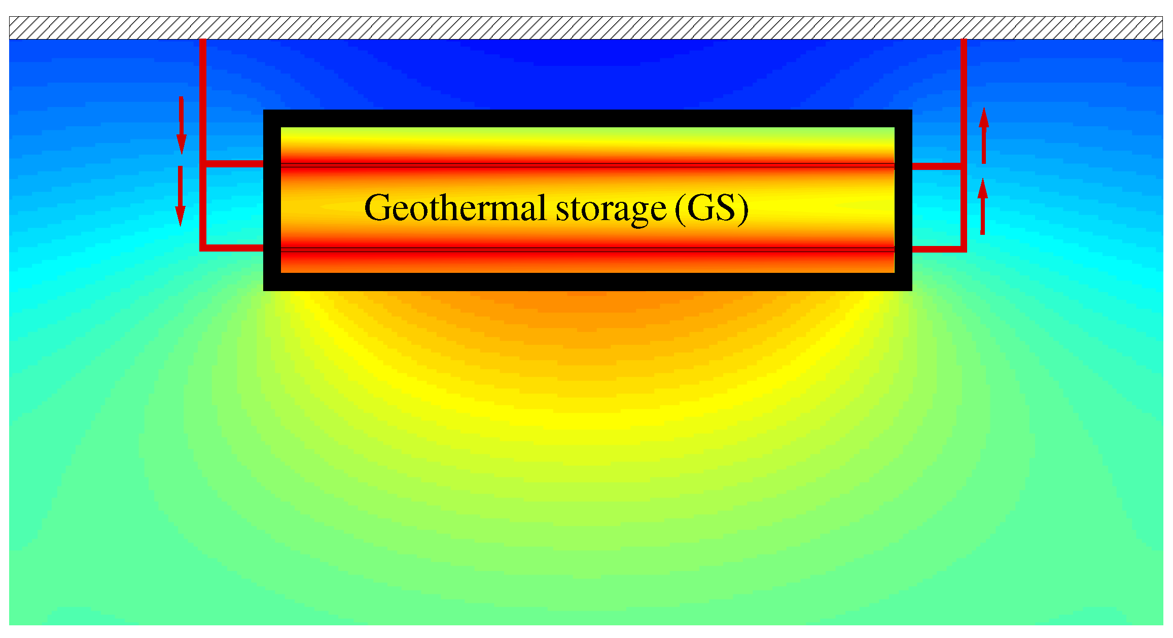
2. Dynamics of Spatial Temperature Distribution in a Geothermal Storage

The setting is based on [10], Section 2. For self-containedness and the convenience of the reader, we recall in this section the description of the model.

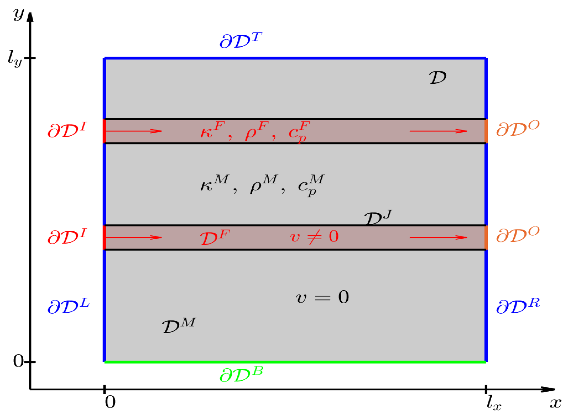
2.1. Two-Dimensional Model

The domain of the geothermal storage is assumed to be a rectangular cuboid for which a two-dimensional rectangular cross-section is considered. We denote by $T=T(t,x,y)$ the temperature measured in Celsius at time $t\in [0,t_E]$ in the point $(x,y)\in \mathcal{D}=(0,l_x)\times (0,l_y)$ with $l_x,l_y$ denoting the width and height of the storage. The domain $\mathcal{D}$ and its boundary $\partial \mathcal{D}$ are depicted in Figure 3. $\mathcal{D}$ is divided into three parts. The first is ${\mathcal{D}}^M$, which is filled with a medium (soil) which is assumed to be homogeneous for simplicity, and characterized by constant material parameters ${\rho }^M,{\kappa }^M$, and $c_p^M$ denoting mass density, thermal conductivity, and specific heat capacity, respectively. The second is ${\mathcal{D}}^F$, it represents the PHXs filled with a fluid (water) with constant material parameters ${\rho }^F,{\kappa }^F$ and $c_p^F$. The fluid moves with time-dependent velocity $v_0\left(t\right)$ along the PHX. For the sake of simplicity, we restrict ourselves to the case, often observed in applications, where the pumps moving the fluid are either on or off. Thus, the velocity $v_0\left(t\right)$ is piecewise constant taking values ${\overline{v}}_0>0$ and zero, only. Finally, the third part is the interface ${\mathcal{D}}^J$ between ${\mathcal{D}}^M$ and ${\mathcal{D}}^F$. Observe that we neglect modeling the wall of the PHX and suppose perfect contact between the PHX and the soil. Details are given in (7) and (8) below. We summarize as follows:

Assumption 1.

1. 

Material parameters of the medium ${\rho }^M,{\kappa }^M,c_p^M$ in the domain ${\mathcal{D}}^M$ and of the fluid ${\rho }^F,{\kappa }^F,c_p^F$ in the domain ${\mathcal{D}}^F$ are constants.

2. 

Fluid velocity is piecewise constant, that is, $v_0\left(t\right)=\left\{\begin{array}{cc}{\overline{v}}_0>0,\hfill & \mathit{pump}\mathit{on},\hfill \\ 0,\hfill & \mathit{pump}\mathit{off}.\hfill \end{array}\right.$

3. 

Perfect contact at the interface between fluid and medium.

Heat Equation

The temperature $T=T(t,x,y)$ in the external storage is governed by the linear heat equation with convection term given by Equation (1), see Welty et al. [12], Chapter 15,

$$\begin{array}{cc}\hfill \rho c_p\frac{\partial T}{\partial t}& =\nabla ·(\kappa \nabla T)-\rho v·\nabla \left(c_{p}T\right),(t,x,y)\in (0,t_E]\times \mathcal{D}\backslash {\mathcal{D}}^J,\hfill \end{array}$$

(1)

where $\nabla =\left(\frac{\partial }{\partial x},\frac{\partial }{\partial y}\right)$ denotes the gradient operator. The first term on the right-hand side describes diffusion while the second represents convection of the moving fluid in the PHXs. Further, $v=v(t,x,y)$$=v_0\left(t\right){(v^x(x,y),v^y(x,y))}^{\top }$ denotes the velocity vector with ${(v^x,v^y)}^{\top }$ being the normalized directional vector of the flow. According to Assumption 1, the material parameters $\rho ,\kappa ,c_p$ depend on the position $(x,y)$ and take the values ${\rho }^M,{\kappa }^M,c_p^M$ for points in ${\mathcal{D}}^M$ (medium) and ${\rho }^F,{\kappa }^F,c_p^F$ in ${\mathcal{D}}^F$ (fluid).

Note that there are no sources or sinks inside the storage and therefore the above heat equation appears without forcing term. Based on this assumption, Equation (1) can be written in a compact form given by Equation (2)

$$\begin{array}{c}\hfill \frac{\partial T}{\partial t}=a\Delta T-v·\nabla T,(t,x,y)\in (0,t_E]\times \mathcal{D}\backslash {\mathcal{D}}^J,\end{array}$$

(2)

where $\Delta =\frac{{\partial }^2}{\partial x^2}+\frac{{\partial }^2}{\partial y^2}$ is the Laplace operator and $a=a(x,y)$ is the thermal diffusivity which is piecewise constant with values $a^{†}=\frac{{\kappa }^{†}}{{\rho }^{†}{c}_p^{†}}$ with $†=M$ for $(x,y)\in {\mathcal{D}}^M$ and $†=F$ for $(x,y)\in {\mathcal{D}}^F$, respectively. The initial condition $T(0,x,y)=T_0(x,y)$ is given by the initial temperature distribution $T_0$ of the storage.

2.2. Boundary and Interface Conditions

For the description of the boundary conditions, the boundary $\partial \mathcal{D}$ is decomposed into several subsets as depicted in Figure 3 representing the insulation on the top and the side, the open bottom, and the inlet and outlet of the PHXs. Further, we have to specify conditions at the interface between PHX and soil. The inlet, outlet, and the interface conditions model the heating and cooling of the storage via PHXs. We distinguish between the two regimes “pump on” and “pump off”. For simplicity, we assume perfect insulation at inlet and outlet if the pump is off. As the focus is on the heat transfer across the open bottom boundary, the losses across the insulated top and side are neglected and perfect insulation is assumed at these boundaries. This leads to the following boundary conditions.

• Homogeneous Neumann condition describing perfect insulation on the top and the side, see Equation (3):

  $$\begin{array}{c}\hfill \frac{\partial T}{\partial \mathfrak{n}}=0,(x,y)\in \partial {\mathcal{D}}^T\cup \partial {\mathcal{D}}^L\cup \partial {\mathcal{D}}^R,\end{array}$$

  (3)

  where $\partial {\mathcal{D}}^L=\left\{0\right\}\times [0,l_y]\backslash \partial {\mathcal{D}}^I$, $\partial {\mathcal{D}}^R=\left\{l_x\right\}\times [0,l_y]\backslash \partial {\mathcal{D}}^O$ and $\partial {\mathcal{D}}^T=[0,l_x]\times \left\{l_y\right\}$ and $\mathfrak{n}$ denotes the outer-pointing normal vector.
• Robin condition describing heat transfer on the bottom, as in Equation (4):

  $$\begin{array}{c}\hfill -{\kappa }^M\frac{\partial T}{\partial \mathfrak{n}}={\lambda }^G(T-T^G\left(t\right)),(x,y)\in \partial {\mathcal{D}}^B,\end{array}$$

  (4)

  with $\partial {\mathcal{D}}^B=[0,l_x]\times \left\{0\right\}$, where ${\lambda }^G>0$ denotes the heat transfer coefficient and $T^G\left(t\right)$ the underground temperature.
• Mixed boundary conditions at the inlet: Here one has to distinguish three cases.

  (i)

  Charging: The pump is on ($v_0>0$), the fluid arrives at the storage with the inlet temperature $T^I\left(t\right)=T_C^I$ which is a given constant, and we can impose a Dirichlet boundary condition.

  (ii)

  Waiting: The pump is off ($v_0=0$), and we set a homogeneous Neumann condition describing perfect insulation.

  (iii)

  Discharging: In this mode, the pump is switched on ($v_0>0$) and the operation of the heat pump must be taken into account. The heat pump transfers the heat from the storage tank to the building’s heating system. It is connected to two circuits in which moving fluids carry heat. A first circuit is connected to the geothermal storage. The fluid from the PHX outlet arrives at the inlet of the heat pump with the temperature ${\overline{T}}^O\left(t\right)$. Here, ${\overline{T}}^O\left(t\right)$ denotes average temperature at the PHX outlet at time t. It is one of the aggregated characteristics which are explained in more detail below, see Equation (22). The heat pump withdraws heat from the fluid so that it leaves the pump at time t at the temperature ${\overline{T}}^O\left(t\right)-\Delta T_{HP}$, and returns to the inlet of the geothermal storage. The quantity $\Delta T_{HP}>0$ is called heat pump spread and assumed to be a given constant. The thermal energy extracted from the fluid in the first circuit is then transferred to the fluid in the second circuit, which is connected to the building’s heating system. Here, the temperature is also raised to a level suitable for the heating system by converting electrical energy into thermal energy.

  Mathematically, this leads to a coupling condition which links the inlet temperature to the average temperature at the PHX outlet via $T^I\left(t\right)=T_D^I\left(t\right)={\overline{T}}^O\left(t\right)-\Delta T_{HP}$.

  Summarizing, we obtain Equation (5):

  $$\begin{array}{c}\hfill \left\{\begin{array}{cccc}\hfill T& =\hfill & T_{\mathcal{C}}^I,\hfill & \mathrm{charging},\hfill \\ \hfill \frac{\partial T}{\partial \mathfrak{n}}& =\hfill & 0,\hfill & \mathrm{waiting},\hfill \\ \hfill T& =\hfill & T_D^I\left(t\right),\hfill & \mathrm{discharging},\hfill \end{array}(x,y)\in \partial {\mathcal{D}}^I.\right.\end{array}$$

  (5)

• “Do Nothing” condition at the outlet in the following sense. If the pump is on ($v_0\left(t\right)>0$), then the total heat flux directed outwards can be decomposed into a diffusive heat flux given by ${\kappa }^F\frac{\partial T}{\partial \mathfrak{n}}$ and a convective heat flux given by $v_0\left(t\right){\rho }^F{c}_p^{F}T$. Since the model parameters ${\kappa }^F,v_0,{\rho }^F{c}_p^F$ in real-world applications are such that the convective heat flux is much larger than the first, see for example below in

  Table 1. Model and discretization parameters.

  Parameters		Values	Units	Parameters		Values	Units
  Geometry				Discretization
  width	$l_x$	10	m	step size x	$h_x$	$0.1$	m
  height	$l_y$	1	m	step size y	$h_y$	$0.01$	m
  depth	$l_z$	10	m	time step	$\tau$	1	s
  height of PHX	$d_P$	$0.02$	m	time horizon	$t_E$	36 and 72	h
  number of PHXs	$n_P$	1 and 3
  Material
  medium (dry soil)				fluid (water)
  mass density	${\rho }^M$	2000	kg/m3		${\rho }^F$	998	kg/m3
  specific heat capacity	$c_p^M$	800	J/(kg·K)		$c_p^F$	4182	J/(kg·K)
  thermal conductivity	${\kappa }^M$	$1.59$	W/(m·K)		${\kappa }^F$	$0.60$	W/(m·K)
  thermal diffusivity	$a^M$	$9.94\times {10}^{-7}$	m2/s		$a^F$	$1.44\times {10}^{-7}$	m2/s
  velocity during pumping	${\overline{v}}_0$	${10}^{-2}$	m/s	inlet temp.: charging	$T_C^I$	40	°C
  heat transfer coefficient	${\lambda }^G$	10	W/(m2·K)	heat pump spread	$\Delta T_{HP}$	3	K
  initial temperature	$T_0$	10 and 35	°C	underground temp.	$T^G$	15	°C

  , we neglect the diffusive heat flux. This leads to a homogeneous Neumann condition, expressed by Equation (6)

  $$\begin{array}{c}\hfill \frac{\partial T}{\partial \mathfrak{n}}=0,(x,y)\in \partial {\mathcal{D}}^O.\end{array}$$

  (6)
  If the pump is off, then we assume (as already for the inlet) perfect insulation, which is also described by the above condition.
• Smooth heat flux at interface ${\mathcal{D}}^J$ between fluid and soil leading to a coupling condition given by Equation (7):

  $$\begin{array}{c}\hfill {\kappa }^F\frac{\partial T^F}{\partial \mathfrak{n}}={\kappa }^M\frac{\partial T^M}{\partial \mathfrak{n}},(x,y)\in {\mathcal{D}}^J.\end{array}$$

  (7)
  Here, $T^F,T^M$ denote the temperature of the fluid inside the PHX and of the soil outside the PHX, respectively. Moreover, it is assumed that the contact between the PHX and the medium is perfect which leads to a smooth transition of the temperature given by Equation (8).

  $$\begin{array}{c}\hfill T^F=T^M,(x,y)\in {\mathcal{D}}^J.\end{array}$$

  (8)

3. Discretization of the Heat Equation

Now, we sketch the discretization of the heat Equation (2) together with the boundary and interface conditions given in (3) through (8) using upwind finite difference schemes as in [14]. Details are provided in [10], Section 3 and 4. This is done in two steps. In the first step, semidiscretization is used to approximate the spatial derivatives by their respective finite differences. This approach is also known as “method of lines” and leads to a high-dimensional system of ODEs for the temperatures at the grid points. In the second step, also time is discretized resulting in an implicit finite difference scheme.

3.1. Semidiscretization of the Heat Equation

The spatial domain is discretized by the means of a mesh with grid points $(x_i,y_j)$ where $x_i=i{h}_x,y_j=j{h}_y,i=0,\dots ,N_x,j=0,\dots ,N_y.$ Here, $N_x$ and $N_y$ denote the number of grid points while $h_x=l_x/N_x$ and $h_y=l_y/N_y$ are the step sizes in x and y-direction, respectively. We denote by $T_{ij}\left(t\right)\simeq T(t,x_i,y_j)$ the semidiscrete approximation of the temperature and by $v_0\left(t\right){(v_{ij}^x,v_{ij}^y)}^{\top }=v_0\left(t\right){(v^x(x_i,y_j),v^y(x_i,y_j))}^{\top }=v(t,x_i,y_j)$ the velocity vector at the grid point $(x_i,y_j)$ at time t.

For the sake of simplification of our analysis, we restrict ourselves to the following assumption on the arrangement of PHX and impose conditions on the location of grid points along the PHX.

Assumption 2.

1. 

There are $n_P\in \mathbb{N}$ straight horizontal PHXs, the fluid moves in positive x-direction.

2. 

The interior of the PHXs contains grid points.

3. 

Each interface between medium and fluid contains grid points.

We approximate the spatial derivatives in the heat equation, the boundary and interface conditions by finite differences as in [10], Sections 3.1–3.3, where we apply upwind techniques for the convection terms. The result is the system of ODEs (9) (given below) for a vector function $Y:[0,T]\to {\mathbb{R}}^n$ collecting the semidiscrete approximations $T_{ij}\left(t\right)$ of the temperature $T(t,x_i,y_j)$ in the “inner” grid points, that is, all grid points except those on the boundary $\partial \mathcal{D}$ and the interface ${\mathcal{D}}^J$. For a model with $n_P$ PHXs, the dimension of Y is $n=(N_x-1)(N_y-2n_P-1)$, see [10].

Using the above notation, the semidiscretized heat Equation (2) together with the given initial, boundary and interface conditions is given by Equation (9).

$$\begin{array}{c}\hfill \frac{dY\left(t\right)}{dt}=\tilde{A}\left(t\right)Y\left(t\right)+B\left(t\right)g\left(t\right),t\in (0,T],\end{array}$$

(9)

with the initial condition $Y\left(0\right)=y_0$, where the vector $y_0\in {\mathbb{R}}^n$ contains the initial temperatures $T_0(·,·)$ at the corresponding grid points. The system matrix A resulting from the spatial discretization of the convection and diffusion term in the heat Equation (2) together with the mixed boundary conditions is given by Equation (10).

$$\begin{array}{c}\hfill \tilde{A}=\left\{\begin{array}{cc}A+B_1{C}^O,\hfill & \mathrm{discharing},\hfill \\ A\hfill & \mathrm{otherwise},\hfill \end{array}\right.\end{array}$$

(10)

where $C^O\in {\mathbb{R}}^{1\times n}$ is the output matrix given in Equation (A14). The matrix A has the tridiagonal structure as shown in Equation (11):

$$\begin{array}{c}\hfill A=\left(\begin{array}{cccccc}{A}_L& D^{+}& & & & \\ D^{-}& A_M& D^{+}\\ & D^{-}& A_M& D^{+}\\ & & \ddots & \ddots & \ddots & \\ & & & D^{-}& A_M& D^{+}\\ & & & & D^{-}& A_R\end{array}\right)\end{array}$$

(11)

and consists of $(N_x-1)\times (N_x-1)$ block matrices of dimension $q=N_y-2n_P-1$. The block matrices $A_L,A_M,A_R$ on the diagonal have a tridiagonal structure and are given in [10], Table 1. The block matrices on the subdiagonals ${\mathcal{D}}^{\pm }\in {\mathbb{R}}^{q\times q}$, $i=1,\dots ,N_x-1$, are diagonal matrices and given in [10], Equation (20).

As a result of the discretization of the mixed boundary conditions at the inlet and the Robin condition at the bottom boundary, we get the function $g:[0,T]\to {\mathbb{R}}^2$ called input function and the $n\times 2$ matrix $\mathcal{B}=({\mathcal{B}}_1,{\mathcal{B}}_2)$ called input matrix. The entries of the input matrix ${\mathcal{B}}_{lr},l=1,\dots ,n,r=1,2,$ are derived in [10], Section 3.4 and are given by Equation (12).

$$\begin{array}{c}\hfill \begin{array}{cc}\hfill B_{l1}=B_{l1}\left(t\right)=\left\{\begin{array}{cc}0,\hfill & \mathrm{waiting},\hfill \\ \frac{a^F}{h_x^2}+\frac{{\overline{v}}_0}{h_x},\hfill & \mathrm{otherwise},\hfill \end{array}\right.& l=\mathcal{K}(1,j),(x_0,y_j)\in {\mathcal{D}}^I,\hfill \\ B_{l2}=\frac{{\lambda }^G{h}_y}{{\kappa }^M+{\lambda }^G{h}_y}{\beta }^M,\hfill & l=\mathcal{K}(i,1),(x_i,y_0)\in {\mathcal{D}}^B,\hfill \end{array}\end{array}$$

(12)

with ${\beta }^M=a^M/h_y^2$. The entries for other l are zero. Here, $\mathcal{K}$ denotes the mapping $(i,j)\mapsto l=\mathcal{K}(i,j)$ of pairs of indices of grid point $(x_i,y_j)\in \mathcal{D}$ to the single index $l\in \{1,\dots ,n\}$ of the corresponding entry in the vector Y. The input function reads as $g\left(t\right)={({\tilde{T}}^I,T^G\left(t\right))}^{\top }$, where ${\tilde{T}}^I$ is given by Equation (13):

$$\begin{array}{c}\hfill {\tilde{T}}^I=\left\{\begin{array}{cc}{T}_C^I,& \mathrm{charging},\hfill \\ 0,& \mathrm{waiting},\hfill \\ -\Delta T_{HP},& \mathrm{discharging}.\hfill \end{array}\right.\end{array}$$

(13)

Recall that $T_C^I$ is the inlet temperature of the PHX during charging and $\Delta T_{HP}$ is the heat pump spread, and $T^G$ is the underground temperature.

3.2. Full Discretization

After discretizing the heat Equation (2) with respect to spatial variables, we will now also discretize the temporal derivative and derive a family of implicit finite difference schemes.

We introduce the notation $N_{\tau }$ for the number of grid points in the t-direction, $\tau =t_E/N_{\tau }$ the time step, and $t_k=k\tau ,k=0,\dots ,N_{\tau }$. Let $A^k,B^k,g^k,v_0^k$ be the values of $A\left(t\right),B\left(t\right),g\left(t\right),v_0\left(t\right)$ at time $t=t_k$, respectively. Further, we denote by $Y^k={(Y_1^k,\dots ,Y_n^k)}^{\top }$ the discrete-time approximation of the vector function $Y\left(t\right)$ at time $t=t_k$. Discretizing the temporal derivative in (9) with the forward difference gives Equation (14):

$$\begin{array}{c}\hfill \frac{dY\left(t_k\right)}{dt}=\frac{Y^{k+1}-Y^k}{\tau }+O\left(\tau \right).\end{array}$$

(14)

Here, the Landau symbol $O\left(\tau \right)$ indicates that there is a linear approximation order of the finite difference approximation of the derivative $dY\left(t_k\right)/dt$. Substituting (14) into (9) and replacing the right hand side of (9) by a linear combination of the values at time $t_k$ and $t_{k+1}$ with the weight $\theta \in [0,1]$, gives the general $\theta$-implicit finite difference scheme, as shown in Equation (15):

$$\begin{array}{c}\hfill \frac{Y^{k+1}-Y^k}{\tau }=\theta [\tilde{A}\left(t_{k+1}\right)Y^{k+1}+B\left(t_{k+1}\right)g^{k+1}]+(1-\theta )[\tilde{A}\left(t_k\right)Y^k+B\left(t_k\right)g^k]\end{array}$$

(15)

for which we provide in [10], Section 4a detailed stability analysis. For our numerical simulations in Section 5 Equation (16) is used, which is an explicit scheme obtained from Equation (15), for $\theta =0$, and given by the recursion

$$\begin{array}{cc}\hfill Y^{k+1}& =({\mathbb{I}}_n+\tau {\tilde{A}}^k)Y^k+\tau B^k{g}^k,k=0,\dots ,N_{\tau }-1,\hfill \end{array}$$

(16)

with the initial value $Y^0=Y\left(0\right)$ and the notation ${\mathbb{I}}_n$ is the $n\times n$ identity matrix. The advantage of an explicit scheme is that it avoids the time-consuming solution of systems of linear equations but one has to satisfy stronger conditions on the time step $\tau$ to ensure stability of the scheme. In [10], Theorem 2, we show that the above explicit scheme is stable if the time step $\tau$ satisfies the condition in Equation (17).

$$\begin{array}{c}\hfill \tau \le {\left(2max\{a^F,a^M\}\left(\frac{1}{h_x^2}+\frac{1}{h_y^2}\right)+\frac{{\overline{v}}_0}{h_x}\right)}^{-1}.\end{array}$$

(17)

4. Aggregated Characteristics

The description of the input-output behavior of the geothermal storage does not necessarily need the complete information about the spatio-temporal temperature distribution in the geothermal storage that can be computed using the numerical methods described in Section 3. For that purpose, it is sufficient to know only a few aggregated characteristics of the temperature distribution which can be computed via post-processing as in [10], Section 5. For self-containedness and the convenience of the reader we sketch some of these aggregated characteristics and describe their approximate computation based on the solution vector Y of the finite difference scheme.

4.1. Aggregated Characteristics Related to the Amount of Stored Energy

Let us consider aggregated characteristics that can be described by the average temperature in some subdomain of the storage, which are related to the amount of stored energy in that domain. For that purpose, let $\mathcal{B}\subset \mathcal{D}$ be a generic subset of the 2D computational domain and denote by $\left|\mathcal{B}\right|={\int \int }_{\mathcal{B}}dxdy$ the area of $\mathcal{B}$. Then $W_{\mathcal{B}}\left(t\right)=l_z{\int \int }_{\mathcal{B}}\rho c_{p}T(t,x,y)dxdy$ represents the thermal energy contained in the 3D spatial domain $\mathcal{B}\times [0,l_z]$ at time $t\in [0,t_E]$. For $0\le t_0<t_1\le t_E$, the difference $G_{\mathcal{B}}(t_0,t_1)=W_{\mathcal{B}}\left(t_1\right)-W_{\mathcal{B}}\left(t_0\right)$ is the gain of thermal energy during the period $[t_0,t_1]$. Positive values correspond to warming of $\mathcal{B}$, negative values indicate cooling. Further, $-G_{\mathcal{B}}(t_0,t_1)$ represents the magnitude of the loss of thermal energy.

For $\mathcal{B}={\mathcal{D}}^{†},†=M,F$, we can use that the material parameters on ${\mathcal{D}}^{†}$ equal the constants $\rho ={\rho }^{†},c_p=c_p^{†}$. Then, the corresponding gains of thermal energy $G^{†}$ and the average temperatures ${\overline{T}}^{†}$ of the storage medium ($†=M$) and the fluid ($†=F$), respectively. are given by Equations (18) and (19),

$$\begin{array}{cc}\hfill G^{†}=G^{†}(t_0,t_1)& =G_{{\mathcal{D}}^{†}}(t_0,t_1)={\rho }^{†}{c}_p^{†}\left|{\mathcal{D}}^{†}\right|l_z({\overline{T}}^{†}\left(t_1\right)-{\overline{T}}^{†}\left(t_0\right)),\hfill \end{array}$$

(18)

$$\begin{array}{cc}\hfill {\overline{T}}^{†}\left(t\right)& =\frac{1}{|{\mathcal{D}}^{†}|}\underset{{\mathcal{D}}^{†}}{\int \int }T(t,x,y)dxdy,†=M,F.\hfill \end{array}$$

(19)

With the help of ${\overline{T}}^M$ and ${\overline{T}}^F$, one can derive the average temperature ${\overline{T}}^S$ in the whole storage which is given in Equation (20)

$$\begin{array}{c}\hfill {\overline{T}}^S\left(t\right)=\frac{1}{\left|\mathcal{D}\right|}\left({\overline{T}}^M\left(t\right)|{\mathcal{D}}^M|+{\overline{T}}^F\left(t\right)|{\mathcal{D}}^F|\right).\end{array}$$

(20)

Further, the total gain in the storage denoted by $G^S$ is obtained by $G^S=G^S(t_0,t_1)=G^M(t_0,t_1)+G^F(t_0,t_1).$

4.2. Aggregated Characteristics Related to the Heat Flux at the Boundary

We now turn to the convective heat flux at the inlet and outlet boundary and the heat transfer at the bottom boundary. Consider be a generic curve $\mathcal{C}\subset \partial \mathcal{D}$ on the boundary and denote by $\left|\mathcal{C}\right|={\int }_{\mathcal{C}}ds$ the curve length. The rate at which the energy is injected or withdrawn via the PHX is given by Equation (22),

$$\begin{array}{c}\hfill \begin{array}{cc}\hfill R^P\left(t\right)& ={\rho }^{†}{c}_p^{†}{v}_0\left(t\right)\left[{\int }_{{\mathcal{D}}^I}T(t,x,y)ds-{\int }_{{\mathcal{D}}^O}T(t,x,y)ds\right]\hfill \\ \hfill & ={\rho }^{†}{c}_p^{†}{v}_0\left(t\right)|\partial {\mathcal{D}}^O|\left[T^I\left(t\right)-{\overline{T}}^O\left(t\right)\right],\hfill \end{array}\end{array}$$

(21)

where ${\overline{T}}^O$ denotes the average temperature at the outlet boundary given in Equation (22)

$$\begin{array}{cc}\hfill {\overline{T}}^O\left(t\right)& =\frac{1}{|\partial {\mathcal{D}}^O|}{\int }_{\partial {\mathcal{D}}^O}T(t,x,y)ds.\hfill \end{array}$$

(22)

Above we used the assumptions of horizontal PHXs so that $|\partial {\mathcal{D}}^I|=|\partial {\mathcal{D}}^O|$, and of a uniformly distributed inlet temperature at the inlet boundary $\partial {\mathcal{D}}^I$. Recall that at time t the fluid moves with velocity $v_0\left(t\right)$, it arrives at the inlet with temperature $T^I\left(t\right)$ and leaves at the outlet with the average temperature ${\overline{T}}^O\left(t\right)$. Given an interval of time $[t_0,t_1]$, the quantity $G^P=G^P(t_0,t_1)=l_z{\int }_{t_0}^{t_1}{R}^P\left(t\right)dt$ measures the amount of heat injected ($G^P>0$) to or withdrawn ($G^P<0$) from the storage by the convection of the fluid.

Finally, Equation (23) defines the rate of heat transfer due to diffusion via the bottom boundary,

$$\begin{array}{c}\hfill R^B\left(t\right)={\int }_{{\mathcal{D}}^B}{\kappa }^M\frac{\partial T}{\partial \mathfrak{n}}ds={\int }_{{\mathcal{D}}^B}{\lambda }^G(T^G\left(t\right)-T(t,x,y))ds={\lambda }^G|\partial {\mathcal{D}}^B|\left(T^G\left(t\right)-{\overline{T}}^B\left(t\right)\right).\end{array}$$

(23)

Here, ${\overline{T}}^{\mathcal{B}}$ is the average temperature at the bottom boundary given in Equation (24)

$$\begin{array}{cc}\hfill {\overline{T}}^{\mathcal{B}}\left(t\right)& =\frac{1}{|\partial {\mathcal{D}}^{\mathcal{B}}|}{\int }_{\partial {\mathcal{D}}^{\mathcal{B}}}T(t,x,y)ds.\hfill \end{array}$$

(24)

The second equation in the first line follows from the Robin boundary condition. Integrating over time leads to the quantity $G^B=G^B(t_0,t_1)=l_z{\int }_{t_0}^{t_1}{R}^B\left(t\right)dt$ which describes the amount of heat transferred via the bottom boundary of the storage.

4.3. Energy Balance

In our model a perfect thermal insulation is assumed at all boundaries except the inlet, outlet and the bottom boundary. At the outlet a homogeneous Neumann condition is imposed to model zero diffusive heat transfer. At the inlet we also have a zero diffusive heat transfer under the reasonable assumption that the temperature in the supply pipe is constant and equals $T^I\left(t\right)$, thus the normal derivative $\frac{\partial T}{\partial \mathfrak{n}}$ is zero. This implies that gains and losses of thermal energy in the storage are caused either by injections or withdrawals via the PHX or by heat transfer via the open bottom boundary. Thus, the total gain $G^S$ can be decomposed to obtain the energy balance given by Equation (25):

$$\begin{array}{c}\hfill G^S=G^M+G^F=G^P+G^B.\end{array}$$

(25)

4.4. Computation of Aggregated Characteristics

Approximations of the aggregated characteristics introduced above can be derived by the using finite difference approximations of the temperature $T=T(t,x,y)$. They can be given in terms of the entries of the vector function $Y\left(t\right)$ satisfying the system of ODEs (9) and containing the semidiscrete finite difference approximations of the temperature in the inner grid points of the computational domain $\mathcal{D}$. Recall that the temperatures on boundary and interface grid points can be determined by linear combinations of the entries of $Y\left(t\right)$.

Let ${\overline{T}}^{†}\left(t\right)$ with $†=M,F,S,O,B$ be one of the average temperatures introduced above. Then the numerical approximation of the defining single and double integrals by quadrature rules leads to approximations by linear combinations of the entries of Y given by Equation (26).

$$\begin{array}{cc}\hfill {\overline{T}}^{†}\left(t\right)& \approx C^{†}Y\left(t\right)\hfill \end{array}$$

(26)

where $C^{†}$ is some $1\times n$-matrix. For the details we refer to Appendix A. The extension to approximations based of the solution of the fully discretized PDE (16) is straightforward using the relation $Y\left(t_k\right)=Y\left(k\tau \right)\approx Y^k,k=0,\dots ,N_{\tau }$.

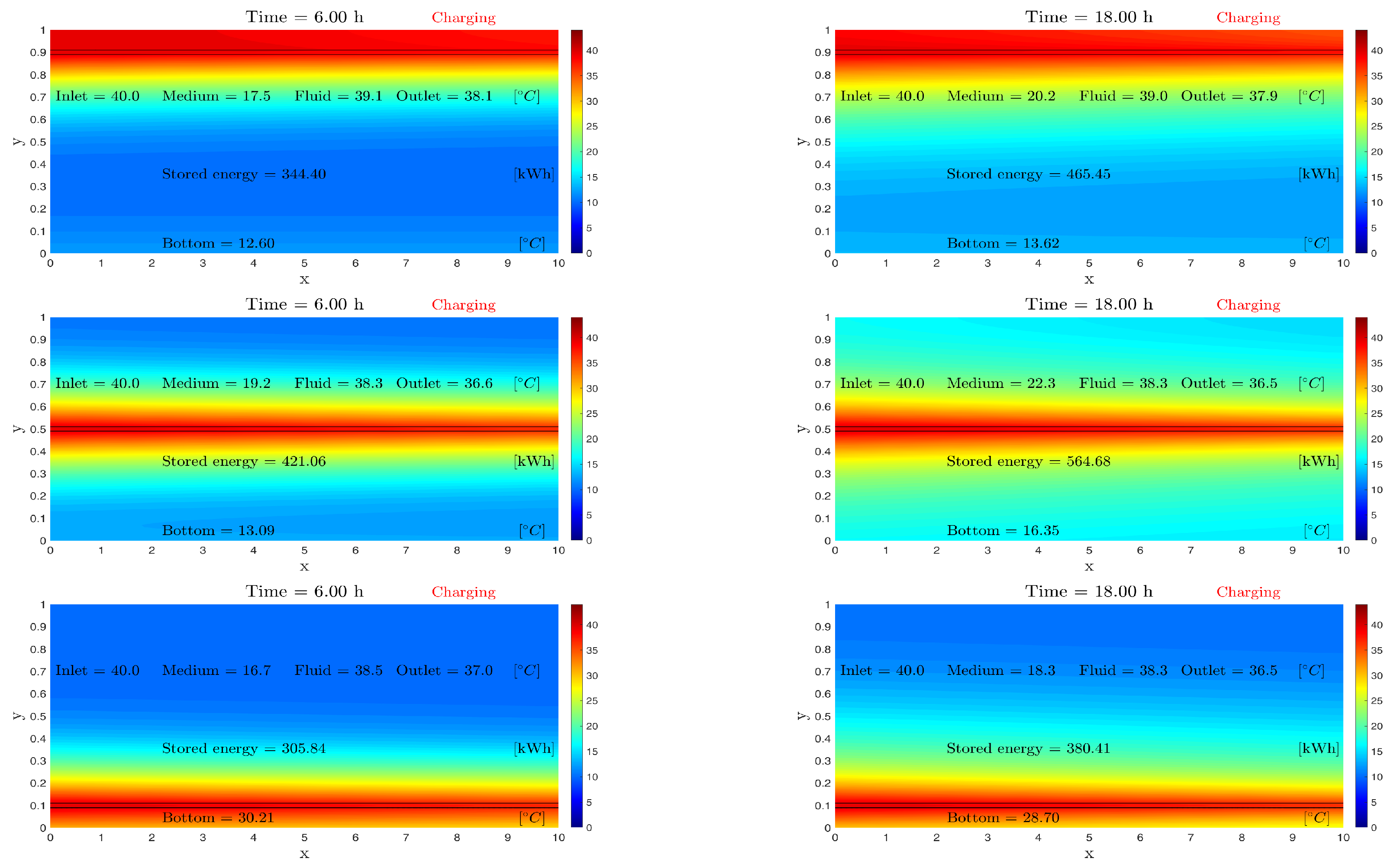
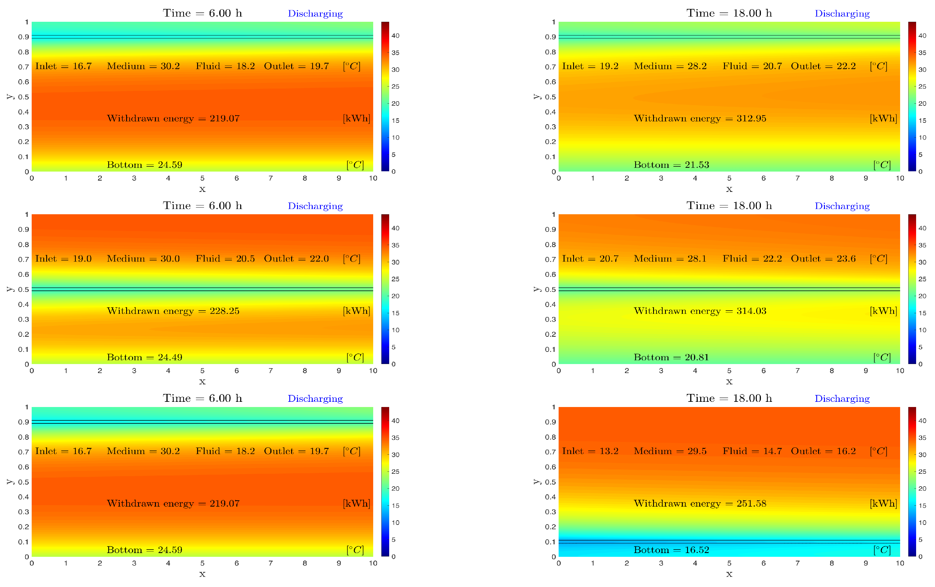
5. Numerical Results

This section presents results of computer simulations based on the finite difference discretization (16) of the heat Equation (2). We work with explicit schemes ($\theta =0$) and determine the spatio-temporal temperature distribution in the storage. Further, the impact of the PHXs topology and vary the number and arrangement of the PHXs is studied. Section 5.2 and Section 5.3 present results for a storage with one and three PHXs, respectively. For these simulations, we also compute and compare certain aggregated characteristics, which were introduced in Section 4 and computed via post processing of the temperature distribution.

5.1. Settings for Numerical Simulation

The model and discretization parameters are given in Table 1. The storage is charged and discharged via PHXs filled with a moving fluid and thermal energy is stored by raising the temperature of the storage medium. Recall the open architecture of the storage, which is only insulated at the top and the side, but not at the bottom. This leads to an additional heat transfer to the underground for which we assume a constant temperature of $T^G\left(t\right)={15}^{°}$. In the simulations, the fluid is assumed to be water while the storage medium is dry soil. First, a simulation is considered in which the storage is charged or discharged over a period of 24 h. Here, the results in which the storage tank is continuously charged or discharged for 6 h and is idle for the rest of the time, are compared with the results in which the storage tank is charged or discharged for $3\times 2$ h and in between there are two waiting periods of 6 h in which the pump is switched off, as can be seen in Figure 6. This helps to mitigate saturation effects in the vicinity of the PHXs reducing the injection and extraction efficiency. We also combine the two 24 h long periods with 3 charging and discharging intervals of 2 h each. The result is a total period of length $t_E=48$ h starting with a storage at temperature $T_0(x,y)={10}^{°}$. Within the the first 24 h, the geothermal storage is charged in three two-hour intervals by the moving fluid arriving at the PHXs inlet at the constant temperature $T^I\left(t\right)=T_{\mathcal{C}}^I$. This is followed by a second period of 24 h in which the storage is discharged at three intervals of two hours, whereby the inlet temperature is $T^I\left(t\right)={\overline{T}}^O\left(t\right)-\Delta T_{HP}$ due to the operation of the heat pump.

During charging, a pump moves the fluid with constant velocity ${\overline{v}}_0$ arriving with constant temperature $T_{\mathcal{C}}^I={40}^{°}$ at the inlet. If this temperature is higher than in the vicinity of the PHX, then a heat flux into the storage medium is induced. During discharging, the fluid from the geothermal storage’s outlet arrives at the inlet of the heat pump with temperature ${\overline{T}}^O\left(t\right)$. Due to the operation of the heat pump, the fluid leaves the heat pump and returns to the inlet of the geothermal storage with the temperature $T_{\mathcal{D}}^I\left(t\right)={\overline{T}}^O\left(t\right)-\Delta T_{HP}$ leading to a cooling of the storage. At the outlet, we impose a vanishing diffusive heat flux, see the “Do Nothing” boundary condition (6), that is, during pumping there is only a convective heat flux. During the waiting periods, the injected heat can propagate to other regions of the storage. Since pumps are off, we have only diffusive propagation of heat in the storage and the transfer over the bottom boundary.

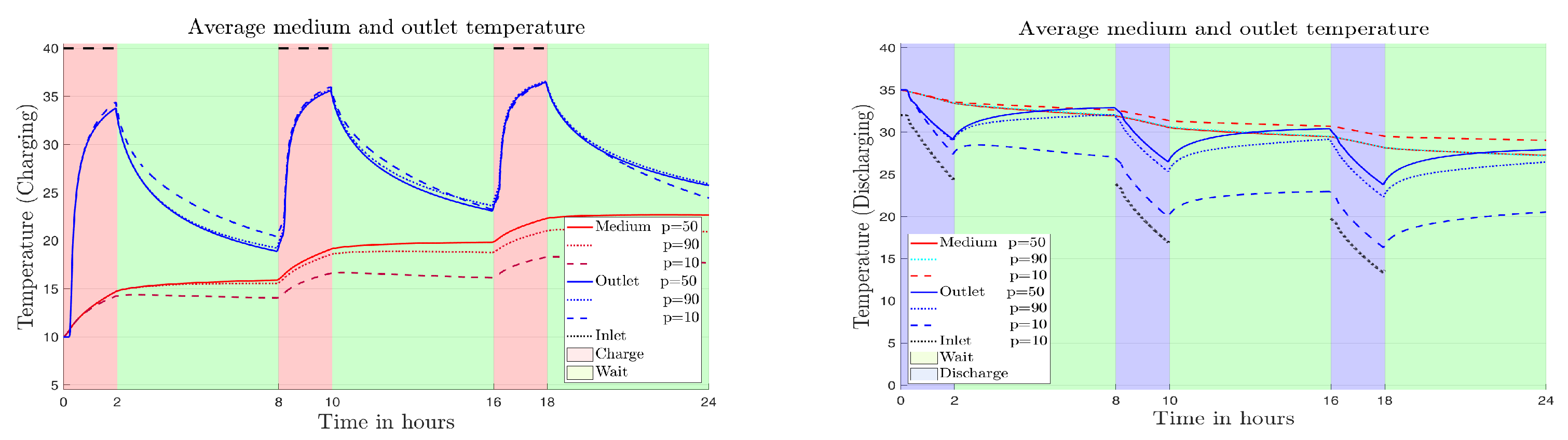
5.2. Storage with One Horizontal Straight PHX for 24 h

Now we present results of simulations for 24 h with one horizontal PHX located at different vertical positions p between the bottom ($p=0$ cm) and the top ($p=l_y=100$ cm) of the storage. We compare the spatial temperature distributions as well as aggregated characteristics such as the average temperature ${\overline{T}}^M\left(t\right)$ in the storage medium, the average outlet temperature ${\overline{T}}^O\left(t\right)$, and the energy $G^M(0,t_E)$ stored in the storage’s medium during a period of $t_E=24$ h. For the charging, we start with a homogeneous initial temperature distribution with $T_0(x,y)={10}^{°}$. In the simulations with discharging, we start with a homogeneous initial temperature distribution with $T_0(x,y)={35}^{°}$. For 24 h, the storage is cooled by the moving fluid arriving at the storage inlet at the inlet temperature $T^I\left(t\right)={\overline{T}}^O\left(t\right)-\Delta T_{HP}$.

Figure 4 shows the spatial distribution of the temperature in the storage after 6 h of continuous charging (left) and discontinuous charging (right), whereas, Figure 5 shows the spatial distribution of the temperature in the storage after 6 h of continuous discharging (left) and discontinuous discharging (right). In both cases, the PHX is located close to the insulated top boundary ($p=90$ cm), in the middle ($p=50$ cm), and close to the bottom boundary ($p=10$ cm), respectively. Recall that the bottom is open and allows for heat transfer to the underground with constant temperature $T^G\left(t\right)={15}^{°}$.

It can be seen that the heating (Figure 4) and cooling (Figure 5) occur mainly in the vicinity of the PHX, and that the temperature in more distant storage areas changes only slightly after 6 h of charging or discharging. Due to the direction of the moving fluid from left to right, warming and cooling in the left part of the storage is slightly stronger than in the right part. A closer inspection of the results shows that, except in the simulation with the PHX close to the bottom boundary ($p=10$ cm), after 6 h of continuous charging the temperatures in the vicinity of that boundary are below the underground temperature $T^G={15}^{°}$. Thus, in addition to the injection of heat via the PHX we also have an inflow of thermal energy from the warmer underground into the storage. This results in a “boundary layer”, which is slightly warmer than in the inner storage region. The reverse effect can be observed during discharging, where close to the bottom boundary the temperature is always above $T^G={15}^{°}$. This induces a heat flux from the storage to the colder underground, which contributes together with the extraction of heat via the PHX to the total loss of thermal energy in the storage.

Figure 6 plots the corresponding average temperatures in the storage medium and at the outlet against time. In Figure 7, we plot in the left panel the thermal energy stored during 24 h of charging against time for vertical positions $p=10,20,\dots ,90$ cm, whereas, the right panel shows the comparison of the stored energy for continuous charging and charging with waiting periods, depending on the vertical PHX position p. It shows that, in the first 2 h of charging or discharging there are almost no visible deviations in the medium temperatures as well as the stored energy, except the case where the pipe is located close to the bottom boundary. However, after 24 h, we can see a clear dependence of the pipe’s vertical position p. Further, for all p, we observe a decaying slope of the curves in the left panel. This can be explained by the “thermal saturation” in the vicinity of the pipe and the slow diffusive propagation of the heat to the more distant regions of the storage. This means that the heat transfer from the IS to the GS is delayed when the PHX environment is at a high temperature. In this case, the PHX fluid exits the GS at almost the same temperature as when it entered, with only a small amount of heat transferred to the storage medium. Conversely, heat transfer from the GS to the IS becomes inefficient if the PHX environment has an inhomogeneous temperature distribution with low temperatures around the PHX. In this case, the PHX fluid can only absorb a small amount of heat from the surrounding storage medium. It can be seen that charging or discharging the storage becomes less efficient after longer periods of operation.

Due to this mode of operation of the charging and discharging processes, heat transfer from the IES to the GES is delayed when the PHX environment is saturated and at a high temperature. In this case, the fluid in the PHX exits the GES at an almost identical temperature to its initial entry, with only a negligible amount of heat transferred to the storage medium. In order to save costs for operating the pumps, it is advantageous in such a case to stop the charging process first and instead wait until the heat in the immediate vicinity of the PHX has spread to colder regions within the GES. Vice versa, the heat transfer from the GES to the IES becomes inefficient if there is a non-homogeneous temperature distribution with low temperatures in the PHX environment. Then, the fluid in the PHX can only absorb a small amount of heat from the storage medium.

5.3. Numerical Results for 48 h

In this subsection, storage architectures with one PHX and three PHXs are considered. For the storage with three PHXs, two different PHXs arrangements are studied. We proceed with the above numerical simulation design but put together the two periods of charging and discharging each of length 24 h. The result is a total period of length $t_E=48$ h starting with a storage at temperature $T_0(x,y)={10}^{°}$. Within the the first 24 h, the storage is charged by the moving fluid arriving at the PHXs inlet with temperature $T_{\mathcal{C}}^I\left(t\right)={40}^{°}$. In the second 36 h, it is discharged using the inlet temperature $T^I\left(t\right)={\overline{T}}^O\left(t\right)-\Delta T_{HP}$. The charging, waiting, and discharging periods can be seen in Figure 9. Contrary to the above simulations, discharging now starts not with a temperature ${35}^{°}$ but with a nonhomogeneous temperature distribution which is obtained after 24 h of charging with several waiting periods.

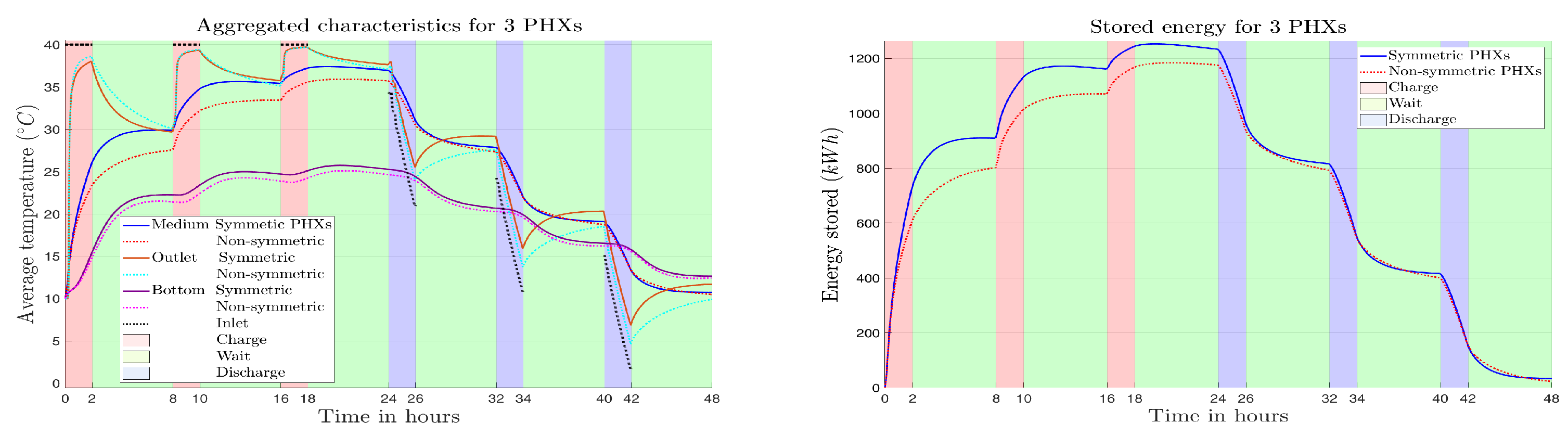
5.3.1. Storage with Three Horizontal Straight PHXs

In this example, we proceed with the above simulation design, including waiting periods.

Figure 8 compares the two storage architectures with three PHXs. In the left panels the PHXs are located symmetrically w.r.t. the vertical mid level, whereas in the right panels the central PHX was moved upwards such that we get a non-symmetric arrangement with two quite close-by PHXs in the upper region. We show snapshots of the spatial temperature distribution during the last charging period (at $t=18$ h), during the waiting period (at $t=28$ h), and during the last discharging period (at $t=42$ h), respectively. These show a strong saturation between the two upper PHXs of the non-symmetric PHXs arrangement while for symmetric PHXs the temperature distribution is much more homogeneous, in particular during the waiting period as it can be seen for time $t=28$ h in the middle right panel of Figure 8.

Figure 9 presents in the left panel aggregated characteristics, which are plotted over time. During the waiting periods after charging, the average outlet temperature decays at a faster rate for symmetric PHXs than for non-symmetric PHXs. For symmetric PHXs, the average storage temperature increases faster during the charging of an almost empty GES than for non-symmetric PHXs. This explains the similar patterns for the gain in stored energy plotted in the right panel of Figure 9. The reason for this is that the storage medium heats up faster and reaches higher temperatures during the charging process between the closely adjacent PHX of the non-symmetrical architecture. It can then absorb less heat from the PHX. In addition, the storage medium around the PHX needs more time to cool down and for the heat propagation to other areas of the GS during the waiting periods.

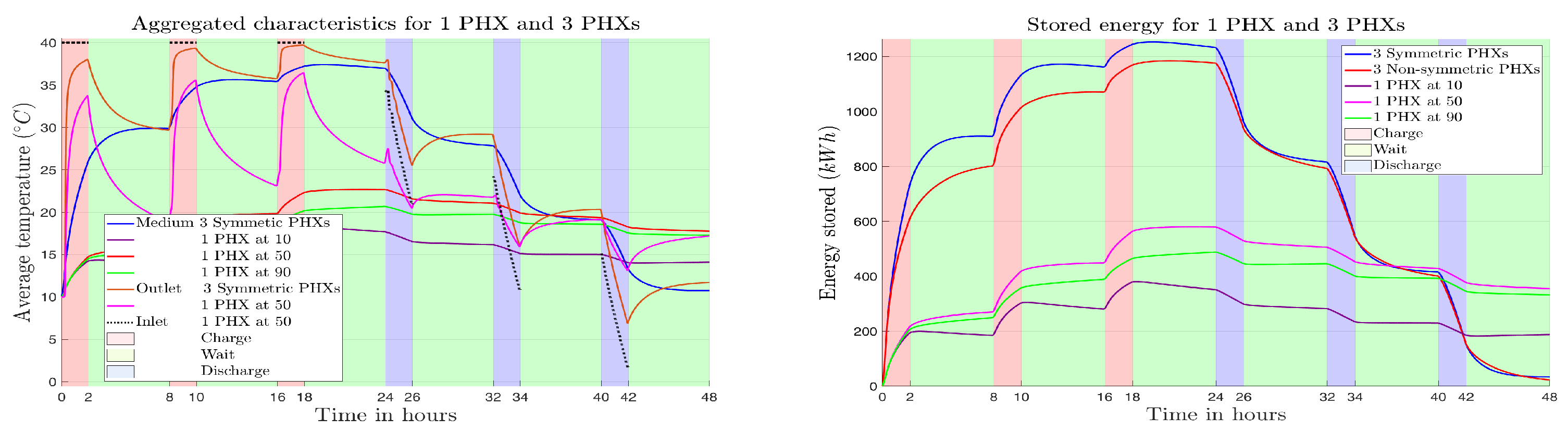
5.3.2. Comparison with One Horizontal Straight PHX

Figure 10 presents in the left panel the comparison of aggregated characteristics for 1 PHX and 3 PHXs, which are plotted over time. In the right panel, we plot the gain of stored energy over time. As expected, the architecture with 3 PHXs is more efficient than that with only one PHX, especially when charging an empty GES with the constant PHX input temperature $T_{\mathcal{C}}^I={40}^{°}$ and when discharging an almost full GES with the help of the heat pump. Here, more energy can be stored or withdrawn in a certain short period of time.

6. Summary and Outlook

We have investigated the numerical simulation of the spatial temperature distribution in a geothermal energy storage and the associated input-output behavior of the storage. The underlying initial boundary value problem for the heat equation with a convection term has been discretised using finite difference schemes. In a large number of numerical simulations, we have shown how theses simulations can support the design and operation of a geothermal storage. Examples are the dependence of the charging and discharging efficiency on the topology and arrangement of PHXs and on the length of charging, discharging, and waiting periods.

The findings of this paper are applied in [13] to study of the cost-optimal management of residential heating systems equipped with a geothermal storage. Mathematically this leads to stochastic optimal control problems. Currently we are working on three-dimensional mathematical models for the spatio-temporal temperature distribution in the geothermal storage, which also take into account a refined topology of the PHXs.

References

1. Guelpa, E.; Verda, V. Thermal energy storage in district heating and cooling systems: A review. Appl. Energy 2019, 252, 113474. [Google Scholar]
2. Kitapbayev, Y.; Moriarty, J.; Mancarella, P. Stochastic control and real options valuation of thermal storage-enabled demand response from flexible district energy systems. Appl. Energy 2015, 137, 823–831. [Google Scholar]
3. Mahmoud, M.; Ramadan, M.; Naher, S.; Pullen, K.; Baroutaji, A.; Olabi, A.G. Recent advances in district energy systems: A review. Therm. Sci. Eng. Prog. 2020, 20, 100678. [Google Scholar] [CrossRef]
4. Dahash, A.; Ochs, F.; Tosatto, A.; Streicher, W. Toward efficient numerical modeling and analysis of large-scale thermal energy storage for renewable district heating. Appl. Energy 2020, 279, 115840. [Google Scholar] [CrossRef]
5. Major, M.; Poulsen, S.E.; Balling, N. A numerical investigation of combined heat storage and extraction in deep geothermal reservoirs. Geotherm. Energy 2018, 6, 1. [Google Scholar] [CrossRef]
6. Regnier, G.; Salinas, P.; Jacquemyn, C.; Jackson, M. Numerical simulation of aquifer thermal energy storage using surface-based geologic modelling and dynamic mesh optimisation. Hydrogeol. J. 2022, 30, 1179–1198. [Google Scholar] [CrossRef]
7. Dincer, I.; Rosen, M.A. Thermal Energy Storage: Systems and Applications; John Wiley & Sons: Hoboken, NJ, USA, 2021. [Google Scholar]
8. Soltani, M.; Moradi Kashkooli, F.; Dehghani-Sanij, A.; Nokhosteen, A.; Ahmadi-Joughi, A.; Gharali, K.; Mahbaz, S.; Dusseault, M. A comprehensive review of geothermal energy evolution and development. Int. J. Green Energy 2019, 16, 971–1009. [Google Scholar]
9. Bähr, M.; Breuß, M. Efficient Long-Term Simulation of the Heat Equation with Application in Geothermal Energy Storage. Mathematics 2022, 10, 2309. [Google Scholar] [CrossRef]
10. Takam, P.H.; Wunderlich, R.; Pamen, O.M. Modeling and simulation of the input–output behavior of a geothermal energy storage. Math. Methods Appl. Sci. 2024, 47, 371–396. [Google Scholar] [CrossRef]
11. Takam, P.H.; Wunderlich, R. Model order reduction for the input–output behavior of a geothermal energy storage. J. Eng. Math. 2024, 148, 12. [Google Scholar] [CrossRef]
12. Welty, J.; Rorrer, G.L.; Foster, D.G. Fundamentals of Momentum, Heat and Mass Transfer; Wiley: Hoboken, NJ, USA, 2019. [Google Scholar]
13. Takam, P.H.; Wunderlich, R. Cost-optimal management of a residential heating system with a geothermal energy storage under uncertainty. arXiv 2025, arXiv:2502.19619. [Google Scholar] [CrossRef]
14. Duffy, D.J. Finite Difference Methods in Financial Engineering: A Partial Differential Equation Approach; John Wiley & Sons: Hoboken, NJ, USA, 2013. [Google Scholar]
Figure 1. Geothermal storage. (Left) Under the new building. (Right) Aside of the building under renovation, see www.ezeit-ingenieure.eu, www.geo-ec.de (accessed on 11 March 2025).
Energies 18 01558 g001
Figure 2. Two-dimensional model of a geothermal storage insulated to the top and the sides while open to the bottom and spatial temperature distribution. The arrows indicate the direction of the moving fluid in the pipe heat exchangers.
Energies 18 01558 g002
Figure 3. Two-dimensional model of the geothermal storage: decomposition of the domain D and the boundary D . The arrows indicate the direction of the moving fluid in the pipe heat exchangers.
Energies 18 01558 g003
Figure 4. Spatial distribution of the temperature in the storage with one horizontal PHX at vertical position p after 6 h of continuous charging (left) and 3 × 2 h of charging with 2 waiting periods of 6 h in between (right). (Top) p = 90 cm. (Middle) p = 50 cm. (Bottom) p = 10 cm.
Energies 18 01558 g004
Figure 5. Spatial distribution of the temperature in the storage with one horizontal PHX at vertical position p after of 6 h of continuous discharging (left) and 3 × 2 h of discharging with 2 waiting periods of 6 h in between (right). (Top) p = 90 cm. (Middle) p = 50 cm. (Bottom) p = 10 cm.
Energies 18 01558 g005
Figure 6. Average temperature in the storage medium T ¯ M and average outlet temperature T ¯ O after 24 h for a storage with one horizontal PHX at different vertical positions. (Left) Charging. (Right) Discharging.
Energies 18 01558 g006
Figure 7. Gain of stored energy for a storage with one horizontal PHX at different vertical positions. (Left) Stored energy during 6 h charging with waiting periods. (Right) Comparison of stored energy after 6 h of continuous charging and charging with waiting periods, respectively, depending on vertical PHX position p.
Energies 18 01558 g007
Figure 8. Spatial distribution of the temperature in the storage with three horizontal PHXs during charging (top), waiting (middle) and discharging (bottom) period. (Left) Symmetric PHXs. (Right) Non-symmetric PHXs.
Energies 18 01558 g008
Figure 9. Storage with three horizontal PHXs during 48 h with charging, waiting and discharging periods. (Left) Comparison of aggregated characteristics T ¯ M , T ¯ O , T ¯ B for symmetric and non-symmetric PHXs. (Right) Gain of stored energy in the geothermal storage.
Energies 18 01558 g009
Figure 10. Comparison of storage with 1 PHX and three horizontal PHXs during 48 h with charging, waiting and discharging periods. (Left) Comparison of aggregated characteristics T ¯ M , T ¯ O for 3 symmetric PHXs and 1 PHX located at 10, 50, and 90. (Right) Comparison of stored energy in the geothermal storage.
Energies 18 01558 g010