Article

A Novel Model for U-Tube Steam Generators for Pressurized Water Reactors

by
Huseyin Emre Sahin
* and
Harun Kemal Ozturk
Mechanical Engineering Department, Pamukkale University, 20160 Denizli, Turkey
*
Author to whom correspondence should be addressed.
Energies 2025, 18(6), 1506; https://doi.org/10.3390/en18061506
Submission received: 24 January 2025 / Revised: 14 March 2025 / Accepted: 16 March 2025 / Published: 18 March 2025
(This article belongs to the Special Issue Advanced Technologies in Nuclear Engineering)

Abstract

:
A novel model was proposed for U-Tube Steam Generators in Pressurized Water Reactors to be utilized in dynamics and control studies. The steam generator was divided into 14 nodes and investigated by applying mass and energy conservation equations in differential form. A system of nonlinear differential equations was obtained. This equation system was numerically simulated using the Julia programming language through a fourth order Runge–Kutta method. Accurate values for thermodynamic properties were taken from the Coolprop library, eliminating the need to take constant values or linear interpolations. A three-element proportional and integral control was applied as the control system in the model. Changes in feedwater flow rate, steam outlet flow rate, primary inlet flow rate, feedwater inlet temperature and primary inlet temperature were investigated, and the response of the steam generator was simulated using the developed model. It was observed that the proposed model gives results for U-Tube Steam Generators comparable to those in the literature and that it can be used in dynamic model and control simulations.

1. Introduction

U-Tube Steam Generators (UTSGs) are significant energy transfer points in Pressurized Water Reactors (PWRs). The main function of a UTSG is to smoothly transfer the heat energy produced by fission reactions in the reactor core to the turbine-generator system that produces electrical energy. This type of steam generator is called a UTSG because the primary loop fluid passes through the inverted U-Tube bundle. In the primary loop of a UTSG, hot water from the reactor runs by circulating through bundles of U-Tubes. In the secondary loop, feedwater enters the steam generator, heats up to the saturation point and changes its phase from liquid to vapor due to heat transfer. It then passes through the riser, separator and dryer sections and leaves the UTSG as almost dry steam [1].
UTSGs have separate sections as water and steam zones. Keeping the water level in the UTSG under control is important for PWRs. The water level of the UTSG must be controlled and kept within a certain height range. In cases where the water level is higher than the desired range, steam quality will decrease and there will be a risk of steam-water droplets entering the turbine section. This causes damage to the turbine blades. Otherwise, if the water level in a UTSG is lower than what it should be, the risk of exposing U-tube bundles to vapor rather than liquid increases. It negatively affects heat transfer between the primary and secondary loops. It will also cause hydrodynamic instability. Due to these problems, accurate control of the UTSG water level is an important operation and control problem for PWR plants. The main problem concerning UTSG water level control is the behavior known as the shrink and swell phenomenon. In case of boiling in UTSGs, steam bubbles occur in the liquid part. This is the main cause of shrink and swell. If the feedwater flow rate increases while the system is operating in steady state, the water level is expected to increase. This is the long-term behavior of the system. But in the short term, adding more water to the fluid in the secondary part of the steam generator will have a cooling effect, reducing the volume of the steam bubbles and causing a temporary decrease in the water level. This is the shrink phenomenon and these reverse dynamics can cause routine controllers to react in the wrong direction. In case the feedwater flow to the UTSG secondary section decreases, a temporary increase occurs before the water level decreases, which is the swell phenomenon and is the opposite of the shrink phenomenon [2,3,4].
When working with large-capacity systems such as nuclear power plants, studies carried out in environments containing radioactive material, high temperature and high-pressure risks are important. Since UTSGs are a significant energy transfer point in these systems, dynamic models and control studies are important. Considering the different operating conditions of the reactor, the proper functioning of the UTSG is necessary for the entire system due to its dynamic structure. For all these reasons, controlling the UTSG water level is of great importance.
There are various studies on UTSGs and PWRs. Irving et al. presented a linear parameter varying model to describe the SG dynamics over the entire operating power range and proposed a model-reference adaptive PID level controller [4]. Ali designed four different models and analyzed them linearly [5]. Naghedolfeizi analyzed a nonlinear and linear model for PWR components and evaluated it to utilize linear simulation [6]. Guimaraes et al. developed a nine-variable model for UTSGs coupled with a three-element controller [7]. Wan et al. developed a dynamic model of an AP1000 steam generator and compared linear and nonlinear models [8]. Qiu et al. designed a nonlinear model and a transfer function model and analyzed water level change [9]. Parlos and Rais implemented H norm with gain scheduled to regulate water level [10]. Salehi et al. developed a μ-synthesized robust controller for the UTSG [11]. Kavaklioglu proposed a predictive control algorithm using support vector regression-based models for controlling the water level of the UTSG [2]. Ansarifar proposed an adaptive dynamic sliding mode control method for the UTSG [12]. Na designed a steam generator water level controller with flow error prediction [13]. Dong et al. used water mass inventory to control the water level of a steam generator [3]. Tan proposed a simple gain-scheduled water level control system designed based on an internal model control principle [14]. Dong et al. designed the state-space model of a UTSG and presented an output feedback dissipation control (OFDC) for water level control [15]. Kothare et al. designed model predictive control by using a linear parameter varying model of the UTSG [16]. Zhao et al. developed a Fluent-based three-dimensional thermal-hydraulic analysis code for a steam generator [17]. Li et al. conducted research on the transition of reverse flow from forced circulation to natural circulation for UTSGs and investigated reverse flow characteristics [18]. Zhang et al. obtained a one-dimensional mathematical model, and it is seen that the exit temperature of the primary side, vapor saturation temperature and mass ratio of the secondary side give compatible results [19]. Qiu et al. studied maintaining the water level of a UTSG within a specific range while power varies greatly, using a fuzzy weighting controller with triangular and trapezoidal membership functions [20]. Chu et al. investigated the effect of reverse flow characteristics on pressure drop in U-tubes under two-phase natural circulation [21]. Hui et al. designed a model by dividing the steam generator into four regions and investigated the heat transfer coefficient distribution, pressure distribution, temperature distribution and velocity distribution of the working environment [22]. Chen et al. proposed a computational model for analyzing the water level of a steam generator, based on cross-calculation and the design and installation characteristics of existing narrow–wide range level transmitters [23]. Zhang et al. developed a code for the thermal-hydraulic design and analysis of a helically coiled tube once-through steam generator, analyzing heat transfer coefficients and pressure drop [24]. Hui proposed fixed-time fractional-order sliding mode controller with a disturbance observer for the U-tube steam generator [25]. Li et al. applied the Model Independent Optimization (MFO) method, based on the Knowledge-Based Historical Gradient-Based Simultaneous Perturbation Stochastic Approach (GK-SPSA), to optimize the performance of the steam generator level control system [26]. Qi et al. conducted a study on the use of artificial intelligence in fault diagnosis techniques in nuclear power plants [27]. Xiao et al. conducted a study on PID control of simplified once-through steam generators [28]. Bolfo et al. developed the 3D-CAD and CFD models of the intermediate heat exchanger installed in nuclear power plant [29]. Li et al. performed non-uniform boiling heat transfer characteristics and calculation evaluation in a U-tube steam generator tube bundle [30]. Ma et al. proposed water level control of U-tube steam generator based on a model-based active disturbance rejection control method [31]. Zhong et al. developed a seven-region lumped-parameter nonlinear dynamic model for a U-tube recirculation nuclear steam generator [32]. Sun et al. proposed transient analysis and dynamic modeling of the steam generator water level for nuclear power plants [33]. Tian et al. proposed a machine -learning-based method for developing a high-degree-of-freedom UTSG thermal model [34].
When the studies in the literature were investigated, it was observed that a group of models for UTSGs are linear. These models are useful for showing the essential behavior of the system. They are easy to implement and do not form a computational burden on the hardware system. In addition, they can show good shrink and swell behavior, as in the model of Irving et al. However, the linear models are not sufficiently detailed, as a true UTSG is naturally nonlinear. Moreover, when the literature on the nonlinear models was investigated, it was observed that some of them do not exactly show the shrink and swell phenomenon. In addition, it was observed that some nonlinear models did not exactly model the water property data since they utilized linear approximations. Ultimately, both nonlinear and linear models show that the computational programs utilized in these investigations need to be updated to a modern computational program language such as Julia.
In this study, a newly modified lumped-parameter nonlinear model was obtained and analyzed for UTSGs. The UTSG system was divided into 14 nodes. Basic conservation equations of mass and energy were applied to these nodes and a nonlinear differential equation system was obtained. A fourth order of Runge–Kutta method was applied to solve the improved nonlinear differential equation system [35]. Julia programming language was utilized as the main language of computation [36]. Microsoft Visual Studio Code (version 1.98.2) was utilized as the development environment. To solve the nonlinear differential equations, thermodynamic properties such as temperature, pressure, enthalpy, specific volume and density were obtained from Coolprop libraries, rather than using linear functions [37]. Coolprop was integrated into the improved model to solve the equation system, allowing accurate thermodynamic properties to be directly accessed and utilized at each time step throughout numerical simulations. A three-element proportional and integral (PI) controller was applied for the improved UTSG model. UTSG water level control simulations were carried out and analyzed under feedwater flow rate, steam outlet flow rate, primary inlet flow rate, feedwater inlet temperature and primary inlet temperature change inputs.
The original contributions of this study can be expressed as follows:
  • A newly modified nodal form: A UTSG was separated into 14 different nodes and modeled using nonlinear differential equations developed from mass and energy basic conservation equations. In previous investigations, some structures of models utilizing fewer nodes showed lower granularity. In the developed model, the primary section has four nodes, the metal tube section has four nodes, and the secondary section has six (subcooled, boiling, downcomer, riser, separator and steam) nodes.
  • Utilization of correct water feature data: Previous investigations in this field generally utilized linear extrapolation and interpolation for water features. As the terms of liquid and steam phases water alter throughout transients, a linear approach may not supply correct feature data. This research utilizes CoolProp features to correctly access the suitable values at each numerical analysis time step throughout the simulation of differential equations. CoolProp is a free C++ library that carries out Fast IAPWS-IF97 (Industrial Formulation) for water and steam along with many other fluids [37].
  • Utilization of Julia programming language: Julia is a comparatively novel programming language made especially for high-performance calculation. It utilizes a nominal-level virtual machine to reach the performance of collected languages, while maintaining the flexibility and speed of improvement of interpreted languages. It can be regarded as a replacement for C or Fortran with a very rich ecosystem like Python (version 3.13.2) [38]. In addition, a fourth order of Runge–Kutta method was applied to solve the developed nonlinear differential equation system in the Julia environment. The model was closed as a loop by adding a three-element PI control system.
This section presents an introduction to the present study. The remaining parts of the article are as follows: Section 2 includes the details of the UTSG system followed by the details of the nodal model including nonlinear differential equations and numerical methods. Section 3 is reserved for simulation results and Section 4 discusses the results.

2. UTSG Model

A novel lumped-parameter model has been developed for UTSGs (Figure 1), which have a complex dynamic structure. Due to the complex dynamic structure of the steam generators, they must be researched at a high level of granularity to improve the precision of the simulation results. For this model, a UTSG is divided into 14 nodes and investigated under three main sections as primary, secondary and metal tube sections (Figure 2). A list of nodes used in this study is given in Table 1.
The nonlinear dynamic model was obtained using basic conservation equations of mass and energy for all nodes. Model studies were carried out by generating and combining a system of nonlinear differential equations with all the conservation equations. This system of equations was analyzed in the Julia environment using a fourth order of Runge–Kutta method. Instant data for thermodynamic properties within the model were used in studies with Coolprop. The developed model was closed as a loop by adding a three-element proportional and integral control system. The parameters of a typical UTSG were taken from the literature (Table S1) [6,7].
Heat transfer occurs between the primary secondary fluids by means of metal tubes in the steam generator. This process involves convection, conduction and convection again. The height at which the secondary fluid reaches its saturation temperature is called the dynamic boundary. The part up to the dynamic boundary is the subcooled region and the region from the dynamic boundary to the end of the heat transfer zone is the boiling region. The dynamic boundary was taken into account when dividing the steam generator into nodes. The primary section is divided into four nodes, the metal tube section is divided into four nodes and the secondary section is divided into six nodes as subcooled, boiling, riser, separator, steam and downcomer regions.
The following assumptions were taken into account when developing this model. The heat transfer from the UTSG to the environment is neglected. The primary fluid is considered incompressible. In the secondary part, the same pressure conditions were accepted for the liquid and the vapor phases. The steam coming out of the steam generator enters the turbine as dry steam. Heat transfer occurs between the primary section, metal tube section and secondary section in the steam generator. It does not occur with the environment or the downcomer.

2.1. Primary Section

The heated water coming from the reactor core runs through the primary section by circulating in U-tubes. The heat energy of the primary fluid is transferred to the metal tube part by convection. Here, four nodes within the U-tubes (P1, P2, P3, P4) are used. In this section, the fluid is incompressible and so it has the same pressure along the tubes and only the energy equation is applied for the primary fluid. The equations obtained with basic conservation equations of energy for P1, P2, P3 and P4 nodes are given as Equations (1), (2), (3) and (4), respectively.
( L 1 d h p 1 d t + h p 1 d L 1 d t ) = ( m ˙ p   h p i h p 1 Q ˙ p 1 ) / ( ρ p A p )
where L 1 is the length of the subcooled region, Q ˙ p 1 is the heat flow rate between P1 and M1 nodes, ρ p is the density of the primary fluid, A p is the primary fluid area, m ˙ p is the primary fluid mass flow rate, h p i is the enthalpy of primary inlet fluid and h p 1 is the enthalpy of P1 fluid.
( L 2 d h p 2 d t h p 2 d L 1 d t ) = ( m ˙ p   h p 1 h p 2 Q ˙ p 2 ) / ( ρ p A p )
where L 2 is the length of boiling region, h p 2 is the enthalpy of P2 fluid and Q ˙ p 2 is the heat flow rate between P2 and M2 nodes.
( L 2 d h p 3 d t h p 3 d L 1 d t ) = ( m ˙ p   h p 2 h p 3 Q ˙ p 3 ) / ( ρ p A p )
where h p 3 is the enthalpy of P3 fluid and Q ˙ p 3 is the heat flow rate between P3 and M3 nodes.
( L 1 d h p 4 d t + h p 4 d L 1 d t ) = ( m ˙ p   h p 3 h p 4 Q ˙ p 4 ) / ( ρ p A p )
where h p 4 enthalpy of P4 fluid and Q ˙ p 4 is the heat flow rate between P4 and M4 nodes.
In the primary section, heat transfer occurs by convection from the primary fluid to the metal tube section. The heat flow rates Q ˙ p 1 , Q ˙ p 2 , Q ˙ p 3 and Q ˙ p 4 are formulated in Equations (5), (6), (7) and (8), respectively.
Q ˙ p 1 = K p A 1 ( T p 1 T m 1 )
where K p is the overall heat transfer coefficient of the primary side and the metal tubes, A 1 is the heat transfer area for L 1 from the primary fluid to the metal tubes, T p 1 is the mean temperature of P1 fluid and T m 1 is the mean temperature of M1 node.
Q ˙ p 2 = K p A 2 ( T p 2 T m 2 )
where A 2 is the heat transfer area for L 2 from the primary fluid to the metal tubes, T p 2 is the mean temperature of P2 fluid and T m 2 is the mean temperature of M2 node.
Q ˙ p 3 = K p A 2 ( T p 3 T m 3 )
where T p 3 is the mean temperature of P3 fluid and T m 3 is the mean temperature of M3 node.
Q ˙ p 4 = K p A 1 ( T p 4 T m 4 )
where T p 4 is the mean temperature of P4 fluid and T m 4 is the mean temperature of M4 node.

2.2. Metal Tube Section

In the metal tube section, metal tubes are considered as the wall parts of the U-tubes. Heat transfer occurs from the primary fluid to the secondary fluid through the metal tube walls. There are four nodes in this section (M1, M2, M3, M4) and the energy equation is applied to derive relevant differential equations. These equations are given as Equations (9), (10), (11) and (12), respectively.
( L 1 d T m 1 d t + T m 1 d L 1 d t ) = ( Q ˙ p 1 Q ˙ m 1 ) / ( ρ m A m 1 C m )
where Q ˙ m 1 is the heat flow rate between M1 and S1, ρ m is the density of metal tube, A m 1 is the area of M1 and M4 and C m is the heat capacity of the metal tubes.
( L 2 d T m 2 d t T m 2 d L 1 d t ) = ( Q ˙ p 2 Q ˙ m 2 ) / ( ρ m A m 2 C m )
where Q ˙ m 2 is the heat flow rate between M2 and S2 and A m 2 is the area of M2 and M3.
( L 2 d T m 3 d t T m 3 d L 1 d t ) = ( Q ˙ p 3 Q ˙ m 3 ) / ( ρ m A m 2 C m )
where Q ˙ m 3 is the heat flow rate between M3 and S2.
( L 1 d T m 4 d t + T m 4 d L 1 d t ) = ( Q ˙ p 4 Q ˙ m 4 ) / ( ρ m A m 1 C m )
where Q ˙ m 4 is the heat flow rate between M4 and S1.
Convection heat transfer equations for this section are given below. Heat transfer in the metal tubes is carried out via conduction. Heat flow rates Q ˙ m 1 , Q ˙ m 2 , Q ˙ m 3 and Q ˙ m 4 for these four nodes are given in Equations (13)–(16).
Q ˙ m 1 = K m A 3 ( T m 1 T s 1 )
where K m is the overall heat transfer coefficient of the metal tubes and the secondary side, A 3 is the heat transfer area for L 1 from the metal tubes to the secondary fluid and T s 1 is the mean temperature of the subcooled region.
Q ˙ m 2 = K m A 4 ( T m 2 T s 2 )
where A 4 is the heat transfer area for L 2 from the metal tubes to the secondary fluid and T s 2 is the mean temperature of the boiling region.
Q ˙ m 3 = K m A 4 ( T m 3 T s 2 )
Q ˙ m 4 = K m A 3 ( T m 4 T s 1 )
The equations for the overall heat transfer coefficients K p (between the primary fluid and inner metal tube walls) and K m (the outer metal tube walls and the secondary fluid), included in heat flow rate equations, are given in Equations (17) and (18) [5,6,7,39].
K p = 1 1 k i + D i 2 c l o g ( D a v g D i )
where k i is the inner convective heat transfer coefficient, c is the metal tube thermal conductivity D i is the inner diameter of the tube and D a v g is the average diameter of the tubes.
K m = 1 1 k o + D o 2 c l o g ( D o D a v g )
where k o is the outer convective heat transfer coefficient and D o is the outer diameter of the tube.

2.3. Secondary Section

In the secondary section, the fluid coming as the feedwater evaporates due to heat transfer along the tubes and leaves the generator as dry steam (St). Feedwater enters the generator through the downcomer (D). The part between the exit of the downcomer and where it reaches the saturation temperature is called the subcooled region (S1). It is assumed that a dynamic boundary is formed at the exit of the subcooled region. The section from this point to the end of the U-tubes length is considered as the boiling region (S2). The liquid–vapor mixture formed in the boiling region is transferred to the separator (S) through the riser (R). From here, the steam part is transferred to the turbine section, while the liquid parts combine with the fluid coming from the feedwater and are transmitted to the downcomer. By using the basic conservation equations of mass and energy for each node, the following equations were obtained and combined.
d L 1 d t = ( m ˙ 1 m ˙ 2 ) / ( ρ s 1 A s )
where m ˙ 1 is the subcooled region inlet mass flow rate, m ˙ 2 is the boiling region inlet mass flow rate, ρ s 1 is the density of the subcooled region fluid and A s is the area of the secondary fluid.
L 1 d h s 1 d t + h s 1 d L 1 d t = ( Q ˙ m 1 + Q ˙ m 4 + m ˙ 1 h d m ˙ 2 h f ) / ( ρ s 1 A s )
where h s 1 is the enthalpy of the subcooled region fluid, h f is the enthalpy of the saturated liquid and h d is the enthalpy of the drum water fluid.
L 2 ρ s 2 d h s 2 d t + L 2 h s 2 d ρ s 2 d t h s 2 ρ s 2 d L 1 d t = ( Q ˙ m 2 + Q ˙ m 3 + m ˙ 2 h f m ˙ 3 h e ) / ( A s )
where ρ s 2 is the density of boiling region fluid, h s 2 is the enthalpy of the boiling region fluid, h e is the enthalpy of the boiling region outlet and m ˙ 3 is the boiling region outlet mass flow rate.
In Equations (19)–(21), the mass and energy equations obtained for nodes S1 and S2 are specified, respectively. All the enthalpy and density values were calculated according to the vapor quality. The mass and energy equations obtained for the water level are given in Equations (22)–(24).
ρ d A d d L d d t = ( m ˙ f w + 1 x e m ˙ 4 m ˙ 1 )
where ρ d is the density of drum water fluid, A d is the drum water fluid area, L d is the drum water level, m ˙ f w is the feedwater mass flow rate, m ˙ 4 is the separator-dryer region inlet mass flow rate and x e is the vapor quality of the boiling region outlet.
ρ d A d h d d L d d t + ρ d A d L d d h d d t = ( m ˙ f w h f w + 1 x e m ˙ 4 h f m ˙ 1 h d )
where h f w is the enthalpy of the feedwater fluid.
( V s t d ρ s t d t ρ s t A d d L d d t ) = ( m ˙ 4 x e m ˙ s o )
where V s t is the volume of the steam node and ρ s t is the density of the steam fluid.
The feedwater flow rate is mixed with the liquid coming from the separator and transferred to the secondary section via the downcomer. When calculating this mass flow rate, the following equation is obtained by using the momentum equation [7].
m ˙ 1 = C 1 ρ d ( L w + L d ) ρ s L w ρ f L d 12
where C 1 is the head loss between annular tank and tube entrance and L w is the accumulation annular tank height.

2.4. Simulations

The UTSG was divided into nodes and a nonlinear model was designed by obtaining equations for all these nodes. Symbolically, this system may be written as the following:
y ˙ ( t ) = f ( y ( t ) , t )
where y ˙ ( t ) is a 14 × 1 vector of functions for the unknown node variables, and f ( y ( t ) , t ) is another 14 × 1 vector of functions, primarily evaluated from the right-hand side of Equations (1)–(24).
Fourth order of Runge–Kutta method is one of the methods used for the numerical solution of nonlinear differential equations. It provides effective and accurate solutions in nonlinear numerical systems [35]. The Runge–Kutta method was applied for model solutions for the obtained nonlinear equation system. The Runge–Kutta equations are as follows:
y n + 1 = y n + 1 6 ( k 1 + 2 k 2 + 2 k 3 + k 4 )
k 1 = h f ( t n ,   y n )
k 2 = h f ( t n + h 2 ,   y n + k 1 2 )
k 3 = h f ( t n + h 2 ,   y n + k 2 2 )
k 4 = h f ( t n + h ,   y n + k 3 )
where t n is the time at step n, h is the time step interval, y n is the solution at t n , y n + 1 is the solution at the next time step and f is the function from Equation (26).
Another important point is the use of correct thermodynamic properties in the model. For the model analysis, thermodynamic properties such as pressure, temperature, density, specific volume, enthalpy and vapor quality were used as Coolprop library calls rather than linear functions. Coolprop’s dynamically linked library was integrated into the model to solve the equation system, allowing all thermodynamic features to be directly captured live at every solution step. This is of great importance in performing model analysis without simplifying and approximating physical actuality [37].
Microsoft Visual Studio Code (version 1.98.2) was utilized as the integrated improvement environment for this study. The Julia language was utilized as the programming language for the analysis studies. It is an open-source program widely used in scientific computing applications. It is frequently used in analysis studies because it provides fast and accurate results [38].

2.5. Three-Element PI Control

A Three-Element PI Control mechanism is used in many PWR plants to regulate the water level in the steam generator [1]. This controller is used to adjust the water level by controlling the feed water flow rate by using three signals: feedwater flow rate, steam outlet flow rate and water level (Figure 3). Two error signals are sent to PI (Proportional and Integral) controller block to regulate the feedwater flow rate adjusting valve position to keep the water level in the steam generator at the desired rate [2,7,40]. The Three-Element PI Controller was applied to close the system as a closed-loop control system.

3. Results

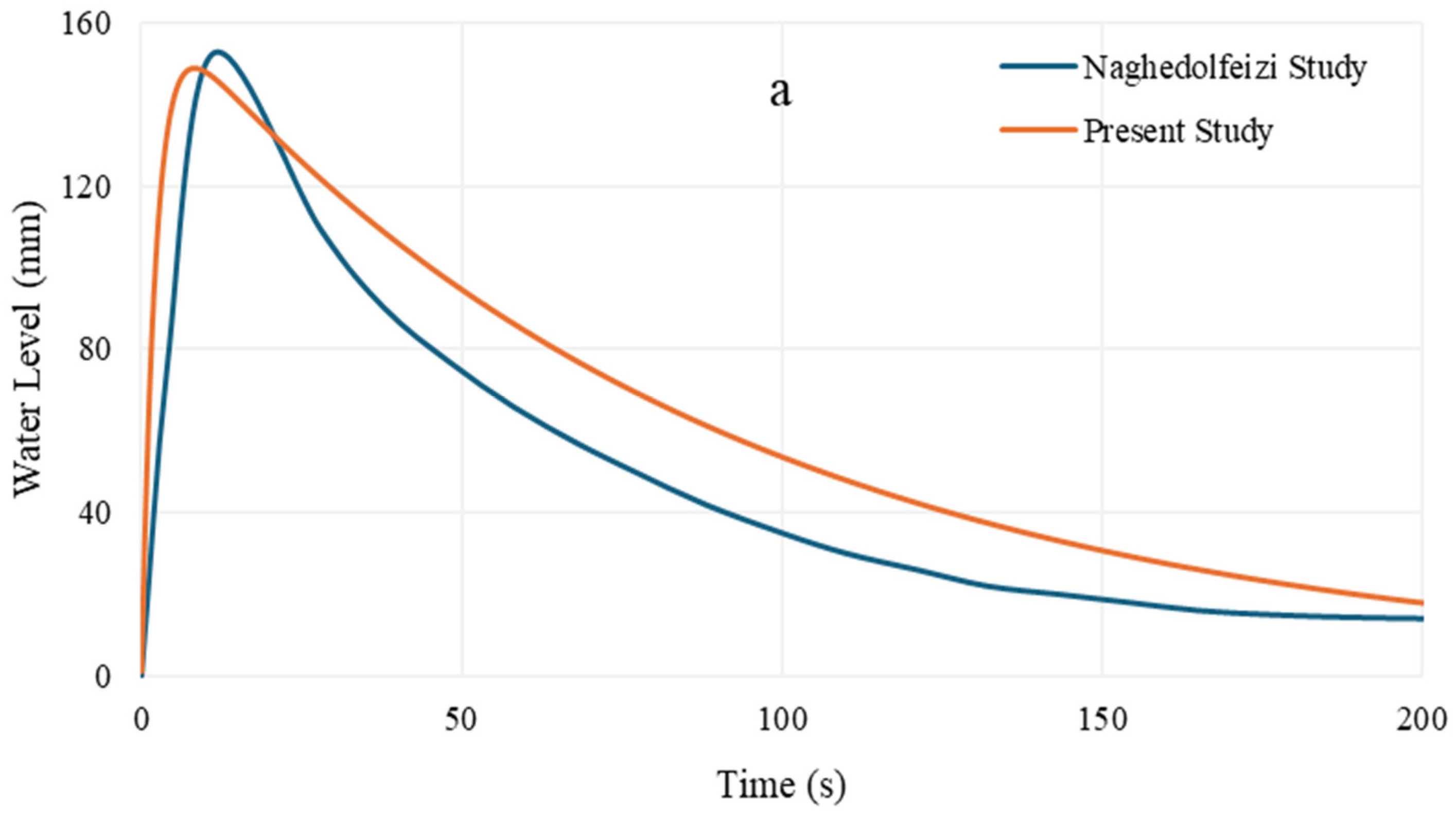
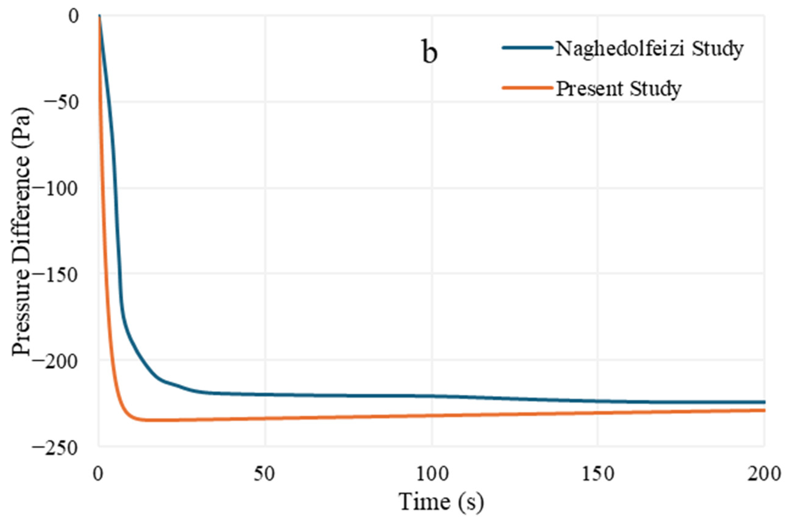
3.1. Validation of the Model

It is difficult to obtain real data directly for UTSGs in PWRs. Data in the literature is used for validation. In this study, validation was performed using the data in Naghedolfeizi’s study [6]. Figure 4 shows a comparison of the water level and pressure difference responses when the steam valve coefficient is increased by 10%. When Figure 4 is considered, it is seen that Naghedolfeizi’s study [6] and the model simulation result here are quite compatible.
Also, the shrink and swell phenomenon, known as inverse dynamic behavior, is one of the most important verification methods in UTSG system numerical analysis. Dong et al. used shrink and swell behavior as verification [36]. Also, in the Westinghouse manual and Wan et al. research, this reverse dynamic behavior is mentioned as a verification method [8,34]. When the water level in Figure 5 and Figure 6, and the pressure difference in Figure 7 and Figure 8 are considered, it is seen that water level behavior shows reverse dynamic behavior, known as the shrink and swell phenomenon mentioned earlier. This reverse dynamic behavior is compatible with studies in the literature [7,8,41,42] and used to validate the model.

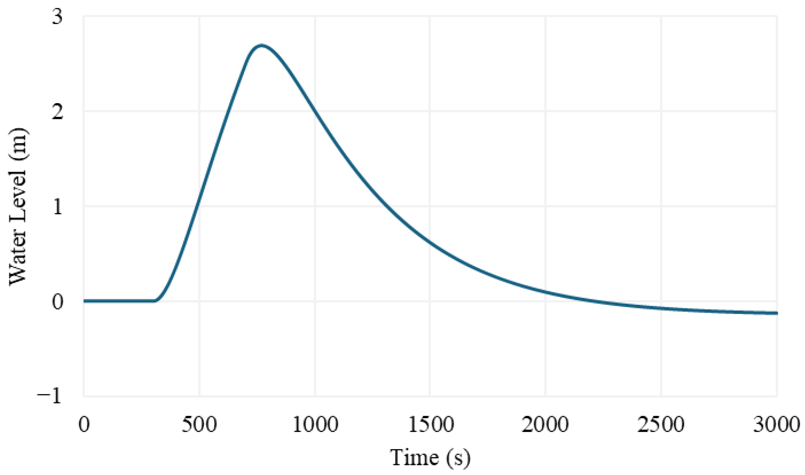
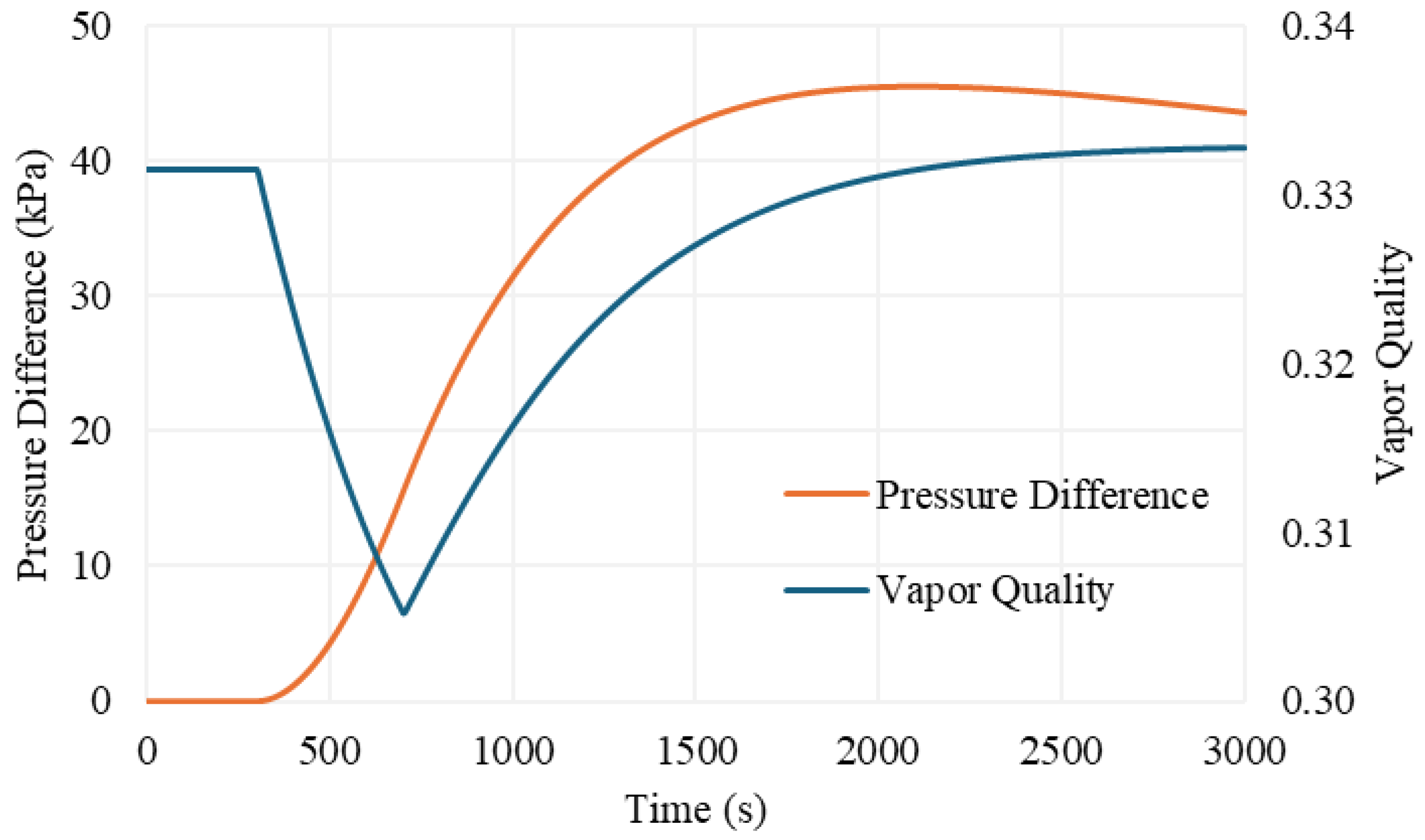
3.2. Results of Simulations

The simulations were first performed with steady-state values. Subsequently, the input data were changed at the 300th second and returned to the initial values at the 700th second, and particularly the water level behavior, pressure difference and vapor quality were researched. All analyses were performed under these time conditions. The time step was used as 0.1 in the model simulations in this study.
In the analysis, the response of water level, vapor quality and pressure difference were evaluated. Results of the model were researched under varied status. The status may be evaluated as unusual behaviors that can form within the PWR plant, like unexpected shutdown, accident analysis and control problems. In the simulations of the model, changes in feedwater flow rate, steam outlet flow rate, feedwater temperature, primary inlet flow rate and primary inlet temperature were researched. The response of the changes, water level, vapor quality and pressure difference values were analyzed and presented.
Firstly, the cases of 5%, 10% and 15% increase in feedwater flow rate were separately simulated. When the feedwater flow rate was increased by 5%, 10% and 15% at the 300th second, the water level suddenly decreased and then returned to the set point due to the controller. When the feedwater flow rate was brought to its initial value at the 700th second, the water level increased and then came to the set point again (Figure 5). In Figure 7, the pressure difference (Figure 7a) in the secondary part and the vapor quality (Figure 7b) value at the exit of the heat transfer zone are shown. At the 300th second, the pressure difference increased and vapor quality decreased. At the 700th second, both values reached a steady-state value. The water level reached the maximum change level at the time of change and immediately after. Then, it returned to a normal level with the controller. The feedwater flow rate increase study has been simulated and compared. These comparison results are presented as the water level in Figure 5, and the pressure difference and vapor quality responses in Figure 7a,b. As the rate of change (5%, 10% and 15%) in the feedwater flow rate increases, water level, pressure difference and steam quality responses change regularly.
Figure 5. Water level responses in cases of 5%, 10% and 15% increases in feedwater flow rate at the 300th second and return to the initial position at the 700th second.
Energies 18 01506 g005
The second simulation is the case of a 5% increase in steam outlet flow rate. When the steam outlet flow rate increased by 5% at the 300th second, the water level suddenly increased (Figure 6), the vapor quality also increased and the pressure difference decreased (Figure 8). After the steam outlet flow rate reached its initial value at the 700th second, all values started to appear at steady-state values. The water level reached the maximum change level at the time of change and immediately after. Then, it returned to a normal level with the controller.
Figure 6. Water level response in the case of a 5% increase in steam outlet flow rate at the 300th second and return to the initial position at the 700th second.
Energies 18 01506 g006
Figure 7. (a) Pressure difference (b) vapor quality responses in cases of 5%, 10% and 15% increases in feedwater flow rate at the 300th second and return to the initial position at the 700th second.
Energies 18 01506 g007
Figure 8. Pressure difference and vapor quality responses in the case of a 5% increase in steam outlet flow rate at the 300th second and return to the initial position at the 700th second.
Energies 18 01506 g008
The third simulation is the case of a 5% increase in primary inlet temperature. When the primary inlet temperature increased by 5% at the 300th second, the water level (Figure 9) and pressure difference began to increase and vapor quality began to decrease (Figure 10). When the primary inlet temperature reached the initial value at the 700th second, the water level and vapor quality returned to the steady-state point and the pressure difference remains at the new state after a while. The maximum change in the water level occurred at the 700th second and then the water level returned to the set point as the temperature was brought back to the initial level.
The fourth simulation is the case of a 5% increase in primary inlet flow rate. When the primary inlet flow rate increases by 5% at the 300th second, the water level (Figure 11) and pressure difference began to increase and vapor quality began to decrease (Figure 12). When the primary inlet temperature reached the initial value at the 700th second, the water level and vapor quality returned to the steady-state point and the pressure difference remained at the new state after a while. The maximum change in the water level occurred at the 700th second and then the water level returned to the set point as the flow rate was brought back to the initial level.
The fifth simulation is the case of a 5% increase in feedwater inlet temperature. When the feedwater inlet temperature increased by 5% at the 300th second, the water level (Figure 13) and pressure difference began to increase and vapor quality began to decrease (Figure 14). When the primary inlet temperature reached the initial value at the 700th second, the water level and vapor quality returned to the steady-state point and the pressure difference remained at the new state after a while.
Five different cases—feedwater flow rate, steam outlet flow rate, primary inlet temperature, primary inlet flow rate and feedwater inlet temperature—change simulations were solved by model, and water level, pressure difference and vapor quality behavior changes were investigated. The reverse dynamic behaviors (shrink and swell) were observed in the feedwater flow rate increase and steam outlet flow rate increase simulations. The maximum changes in the water level, pressure difference and vapor quality were observed in the primary inlet temperature increase simulation.

4. Discussion

In this study, a newly modified model was obtained and a new solution method was implemented. Conservation equations of mass and energy were applied to 14 nodes and a nonlinear differential equation system was obtained. A fourth order of Runge–Kutta method was applied to solve the improved nonlinear differential equation system and the Julia programming language was used. Coolprop was integrated into the improved model to solve the equation system, allowing all accurate thermodynamic properties to be directly accessed and utilized at every time step throughout the numerical simulations. A three-element PI controller was applied for the model. UTSG simulations were carried out and analyzed under feedwater flow rate, steam outlet flow rate, primary inlet flow rate, feedwater inlet temperature and primary inlet temperature change inputs.
The results presented in this study have shown that the model developed throughout this study for UTSGs for PWRs obtained simulations compatible with physical expectance and research. Moreover, it is seen that the three-element PI controller can adjust the water level back to a set point for the disruptions shown here. A model validation study has been carried out successfully. Also, it has been observed that shrink and swell effects are compatible with previous research in the literature. Simulations for the model were made at full power, and it is known that shrink and swell phenomena are more dominant at low levels of power. However, it is hard to get the operating parameters of UTSGs at low levels of power from former research or from real power plants. Finally, the conclusion is reached that the model can be utilized in control and simulation research for PWRs.
In respect of suggestions for future research, depending on the existence of operating data, operating the simulations at various levels of power would be useful to observe this model’s performance during all situations involving real UTSGs. In these systems, comparisons can be made by analyzing different correlations for heat transfer analysis for future works. A potential direction for future research is to implement another type of controller to observe whether the level response can be improved.

Supplementary Materials

The following supporting information can be downloaded at: https://www.mdpi.com/article/10.3390/en18061506/s1, Table S1: UTSG design parameters and constants [6,7].

Author Contributions

Conceptualization, H.E.S. and H.K.O.; methodology, H.E.S.; software, H.E.S.; investigation, H.E.S.; resources, H.E.S.; writing—original draft preparation, H.E.S.; writing—review and editing, H.K.O.; supervision, H.K.O. All authors have read and agreed to the published version of the manuscript.

Funding

This research received no external funding.

Data Availability Statement

The original contributions presented in the study are included in the article/Supplementary Materials, further inquiries can be directed to the corresponding author.

Conflicts of Interest

The authors declare no conflicts of interest.

References

  1. Westinghouse Electric Corporation. The Westinghouse Pressurized Water Reactor Nuclear Power Plant; Westinghouse Electric Corporation: Pittsburgh, PA, USA, 1984. [Google Scholar]
  2. Kavaklioglu, K. Support vector regression model based predictive control of water level of U-tube steam generators. Nucl. Eng. Des. 2014, 278, 651–660. [Google Scholar] [CrossRef]
  3. Dong, W.; Doster, J.M.; Mayo, C.W. Steam Generator control in Nuclear Power Plants by water mass inventory. Nucl. Eng. Des. 2008, 238, 859–871. [Google Scholar] [CrossRef]
  4. Irving, E.; Miossec, C.; Tassart, J. Towards efficient full automatic operation of the PWR steam generator with water level adaptive control. In Proceedings of the 2nd International Conference on Boiler Dynamics and Control in Nuclear Power Stations, Bournemouth, UK, 23–25 October 1980; pp. 309–329. [Google Scholar]
  5. Ali, M.R.A. Lumped Parameter, State Variable Dynamic Models for U-tube Recirculation Type Nuclear Steam Generators. Ph.D. Thesis, University of Tennessee, Knoxville, TN, USA, 1976. Available online: https://trace.tennessee.edu/utk_graddiss (accessed on 15 January 2023).
  6. Naghedolfeizi, M. Dynamic Modeling of a Pressurized Water Reactor Plant for Diagnostics and Control. Master’s Thesis, University of Tennessee, Knoxville, TN, USA, 1990. Available online: https://trace.tennessee.edu/utk_gradthes/2667 (accessed on 15 January 2023).
  7. Guimarães, L.N.F.; da Silva Oliveira, N.; Borges, E.M. Derivation of a nine variable model of a U-tube steam generator coupled with a three-element controller. Appl. Math. Model. 2008, 32, 1027–1043. [Google Scholar] [CrossRef]
  8. Wan, J.; He, J.; Li, S.; Zhao, F. Dynamic modeling of AP1000 steam generator for control system design and simulation. Ann. Nucl. Energy 2017, 109, 648–657. [Google Scholar] [CrossRef]
  9. Qiu, L.; Sun, A.; Wang, H.; Zhang, R.; Jiang, G.; Sun, P.; Wei, X. Study on water level control system of natural circulation steam generator. Prog. Nucl. Energy 2022, 153, 104436. [Google Scholar] [CrossRef]
  10. Parlos, A.G.; Rais, O.T. Nonlinear control of U-tube steam generators via H∞ control. Control Eng. Pract. 2000, 8, 921–936. [Google Scholar] [CrossRef]
  11. Salehi, A.; Kazemi, M.H.; Safarzadeh, O. The μ–synthesis and analysis of water level control in steam generators. Nucl. Eng. Technol. 2019, 51, 163–169. [Google Scholar] [CrossRef]
  12. Ansarifar, G.R. Control of the nuclear steam generators using adaptive dynamic sliding mode method based on the nonlinear model. Ann. Nucl. Energy 2016, 88, 280–300. [Google Scholar] [CrossRef]
  13. Man Gyun Na Design of a steam generator water level controller via the estimation of the flow errors. Ann. Nucl. Energy 1995, 22, 367–376. [CrossRef]
  14. Tan, W. Water level control for a nuclear steam generator. Nucl. Eng. Des. 2011, 241, 1873–1880. [Google Scholar] [CrossRef]
  15. Dong, Z.; Huang, X.; Feng, J. Water-level control for the U-tube steam generator of nuclear power plants based on output feedback dissipation. IEEE Trans. Nucl. Sci. 2009, 56, 1600–1612. [Google Scholar] [CrossRef]
  16. Kothare, M.V.; Mettler, B.; Morari, M.; Bendotti, P.; Falinower, C.M. Level Control in the Steam Generator of a Nuclear Power Plant. 2000. Available online: http://www.edf.fr (accessed on 15 January 2023).
  17. Zhao, X.; Wang, M.; Wu, G.; Zhang, J.; Tian, W.; Qiu, S.; Su, G.H. The development of high fidelity Steam Generator three dimensional thermal hydraulic coupling code: STAF-CT. Nucl. Eng. Technol. 2021, 53, 763–775. [Google Scholar] [CrossRef]
  18. Li, M.; Chen, W.; Hao, J.; Li, W. Experimental and numerical investigations on effect of reverse flow on transient from forced circulation to natural circulation. Nucl. Eng. Technol. 2020, 52, 1955–1962. [Google Scholar] [CrossRef]
  19. Zhang, G.; Zhang, Y.; Yang, Y.; Li, Y.; Sun, B. Dynamic heat transfer performance study of steam generator based on distributed parameter method. Ann. Nucl. Energy 2014, 63, 658–664. [Google Scholar] [CrossRef]
  20. Qiu, L.; Huo, Y.; Zhang, R.; Wang, H.; Jiang, G.; Sun, P.; Wei, X. Research on fuzzy weighted gain scheduling water level control system of U-tube steam generator. Ann. Nucl. Energy 2023, 187, 109812. [Google Scholar] [CrossRef]
  21. Chu, X.; Li, M.; Chen, W.; Hao, J. Investigation on reverse flow characteristics in U-tubes under two-phase natural circulation. Nucl. Eng. Technol. 2020, 52, 889–896. [Google Scholar] [CrossRef]
  22. Hui, J.; Ling, J.; Dong, H.; Wang, G.; Yuan, J. Distributed parameter modeling for the steam generator in the nuclear power plant. Ann. Nucl. Energy 2021, 152, 107945. [Google Scholar] [CrossRef]
  23. Chen, Y.; Xie, Y.; Li, Y.; Ling, J.; Zhou, X. Full-range steam generator’s water level model and analysis method based on cross-calculation. Prog. Nucl. Energy 2021, 133, 103635. [Google Scholar] [CrossRef]
  24. Zhang, Y.; Wang, D.; Lin, J.; Hao, J. Development of a computer code for thermal–hydraulic design and analysis of helically coiled tube once-through steam generator. Nucl. Eng. Technol. 2017, 49, 1388–1395. [Google Scholar] [CrossRef]
  25. Hui, J. Fixed-time fractional-order sliding mode controller with disturbance observer for U-tube steam generator. Renew. Sustain. Energy Rev. 2024, 205, 114829. [Google Scholar] [CrossRef]
  26. Li, X.; Yang, Z.; Yang, Y.; Kong, X.; Shi, C.; Shi, J. GK-SPSA-Based Model-Free Method for Performance Optimization of Steam Generator Level Control Systems. Energies 2023, 16, 8050. [Google Scholar] [CrossRef]
  27. Qi, B.; Liang, J.; Tong, J. Fault Diagnosis Techniques for Nuclear Power Plants: A Review from the Artificial Intelligence Perspective. Energies 2023, 16, 1850. [Google Scholar] [CrossRef]
  28. Xiao, K.; Li, Y.; Yang, P.; Zhang, Y.; Zhao, Y.; Pu, X. Study on IMC-PID Control of Once-Through Steam Generator for Small Fast Reactor. Energies 2022, 15, 7475. [Google Scholar] [CrossRef]
  29. Bolfo, L.; Devia, F.; Lomonaco, G. Nuclear Hydrogen Production: Modeling and Preliminary Optimization of a Helical Tube Heat Exchanger. Energies 2021, 14, 3113. [Google Scholar] [CrossRef]
  30. Li, Z.; Yan, Y.; Fan, G.; Zeng, X.; Hao, S.; Yan, C. Non-uniform boiling heat transfer characteristics and calculation evaluation in U-tube steam generator tube bundle. Energy 2024, 303, 131867. [Google Scholar] [CrossRef]
  31. Ma, Q.; Fan, Z.; Zhang, X.; Sun, P.; Wei, X. Water level control of U-tube steam generator based on model-based active disturbance rejection control method. Ann. Nucl. Energy 2024, 206, 110618. [Google Scholar] [CrossRef]
  32. Zhong, X.; Guo, P.; Zhang, X.; Saeed, M.; Ma, H.; Huang, J.; Yu, J. Development of a seven-region lumped parameter nonlinear dynamic model for U-tube recirculation nuclear steam generator. Ann. Nucl. Energy 2022, 174, 109190. [Google Scholar] [CrossRef]
  33. Sun, X.; Song, F.; Yuan, J. Transient analysis and dynamic modeling of the steam generator water level for nuclear power plants. Prog. Nucl. Energy 2024, 170, 105103. [Google Scholar] [CrossRef]
  34. Tian, Y.; Wang, Y.; Yin, S.; Lu, J.; Hu, Y. Enabling High-Degree-of-Freedom Thermal Engineering Calculations via Lightweight Machine Learning. Energies 2024, 17, 3916. [Google Scholar] [CrossRef]
  35. Butcher, J.C. Numerical Methods for Ordinary Differential Equations, 3rd ed.; Wiley: Hoboken, NJ, USA, 2016. [Google Scholar]
  36. Julia Programming Language Julia. MIT. Available online: https://julialang.org/ (accessed on 1 January 2022).
  37. Bell, I.H.; Wronski, J.; Quoilin, S.; Lemort, V. Pure and Pseudo-Pure Fluid Thermophysical Property Evaluation and the Open-Source Thermophysical Property Library Coolprop. Ind. Eng. Chem. Res. 2014, 53, 2498–2508. [Google Scholar] [CrossRef]
  38. Bezanson, J.; Edelman, A.; Karpinski, S.; Shah, V.B. Julia: A fresh approach to numerical computing. SIAM Rev. 2017, 59, 65–98. [Google Scholar] [CrossRef]
  39. Alramady, A.M.; Al-Sharif, S.; Nafee, S.S. Modeling of UTSG in the Pressurized Water Reactor Using Accurate Formulae of Thermodynamic Properties. J. Appl. Math. Phys. 2021, 9, 947–967. [Google Scholar] [CrossRef]
  40. Kerlin, T.W.; Upadhyaya, B.R. Dynamics and Control of Nuclear Reactors; Elsevier: Amsterdam, The Netherlands, 2019. [Google Scholar]
  41. Dong, Z.; Huang, X.; Feng, J.; Zhang, L. Dynamic model for control system design and simulation of a low temperature nuclear reactor. Nucl. Eng. Des. 2009, 239, 2141–2151. [Google Scholar] [CrossRef]
  42. Westinghouse Westinghouse Technology Systems Manual. 2020. Available online: https://www.nrc.gov/docs/ML2116/ML21166A218.pdf (accessed on 15 January 2023).
Figure 1. Schematics of a typical U-tube Steam Generator.
Energies 18 01506 g001
Figure 2. Nodal model of the UTSG.
Energies 18 01506 g002
Figure 3. Three-Element PI Control diagram.
Energies 18 01506 g003
Figure 4. (a) Water level responses comparison to a 10% step increase in the steam valve coefficient. (b) Pressure difference responses comparison to a 10% step increase in the steam valve coefficient.
Energies 18 01506 g004aEnergies 18 01506 g004b
Figure 9. Water level response in the case of a 5% increase in primary inlet temperature at the 300th second and return to the initial position at the 700th second.
Energies 18 01506 g009
Figure 10. Pressure difference and vapor quality responses in the case of a 5% increase in primary inlet temperature at the 300th second and return to the initial position at the 700th second.
Energies 18 01506 g010
Figure 11. Water level response in the case of a 5% increase in primary inlet flow rate at the 300th second and return to the initial position at the 700th second.
Energies 18 01506 g011
Figure 12. Pressure difference and vapor quality responses in the case of a 5% increase in primary inlet flow rate at the 300th second and return to the initial position at the 700th second.
Energies 18 01506 g012
Figure 13. Water level response in the case of a 5% increase in feedwater inlet temperature at the 300th second and return to the initial position at the 700th second.
Energies 18 01506 g013
Figure 14. Pressure difference and vapor quality responses in the case a of 5% increase in feedwater inlet temperature at the 300th second and return to the initial position at the 700th second.
Energies 18 01506 g014
Table 1. List of nodes.
Node NumberSymbolExplanation
1P1Primary fluid first node
2P2Primary fluid second node
3P3Primary fluid third node
4P4Primary fluid fourth node
5M1Metal tube first node
6M2Metal tube second node
7M3Metal tube third node
8M4Metal tube fourth node
9S1Subcooled region node
10S2Boiling region node
11RRiser node
12SSeparator-Dryer node
13StSteam node
14DDowncomer node
Disclaimer/Publisher’s Note: The statements, opinions and data contained in all publications are solely those of the individual author(s) and contributor(s) and not of MDPI and/or the editor(s). MDPI and/or the editor(s) disclaim responsibility for any injury to people or property resulting from any ideas, methods, instructions or products referred to in the content.

