Abstract
A horizontal-axis H-Darrieus turbine has been developed as a wave energy converter (WEC) to harness energy from coastal waves. In this paper, a semi-analytical method is presented to quantify the wave power contributing to power generation by the H-Darrieus WEC and to assess the distribution of wave power resources. Furthermore, the semi-analytical method incorporating insights from the rotational mechanisms of the H-Darrieus turbine is applied at the Seragaki littoral zone (Okinawa, Japan) and provides the rationale for determining the conceptual design, including installation site, underwater velocity, turbine diameter, rotational speed, and power output. Under a typical swell condition at Seragaki, wave power density of 25 kW/m was calculated right before wave breaking. Given the water depth and underwater flow velocity at this location, a turbine diameter of 2 m, a rotational speed of 120–180 rpm, and a power generation per unit turbine-swept area of 2 kW/m2 were determined as the conceptual design.
1. Introduction
Numerous wave energy converter (WEC) technologies have been developed and deployed worldwide [1,2]. Among them, turbine-type WECs designed to harness energy from coastal waves have been developed in the Okinawa Institute of Science and Technology (OIST) WEC project. In the project, a turbine-type WEC was developed for installation at wave-breaking zones, utilizing the high flow velocities within breaking waves [3,4]. While this approach yielded momentary high power output, the intermittent power output and extreme peak loads posed challenges for stable power generation. Currently, the project has shifted toward the development of a Darrieus-type turbine specifically designed for coastal wave energy conversion [5]. Although the energy source has transitioned from breaking waves to shallow-water waves, the fundamental concepts of the project remain consistent.
Our WEC is designed for direct placement on the seafloor in nearshore areas, which eliminates the need for floating structures and extensive cabling for electricity transmission. This approach significantly reduces installation and maintenance costs while enhancing resilience against extreme weather conditions. Furthermore, wave power is naturally amplified as it approaches the littoral zone until right before wave breaking. The design features a series of simple and small WECs arranged in an array configuration along wave crests. This configuration ensures efficient energy harnessing and wave attenuation. The compact nature of the WECs reduces costs and shortens the development cycle. To maximize power generation, it is important to harness wave kinetic energy directly, avoiding intermediate energy states. Unlike the oscillating mechanisms commonly seen in other WECs, our design employs a rotating mechanism, which is particularly well-suited for the direct conversion of wave energy. This approach not only enhances efficiency but also allows for the application of knowledge from wind turbine technology, utilizing standardized components such as ball bearings and mechanical seals. The compact design minimizes the impact on coastal environments. When installed in an array, the WECs also function as a breakwater, reducing coastal erosion. Since our WEC are mounted on hard seafloors formed by coral reefs in a wave-breaking zone, such as Seragaki (Okinawa, Japan) and Kandooma Island (Maldives), specific measures for sediment transport and shoreline stability are not necessary. In coastal waves, the flow is oscillatory, and there is no steady current directed toward the turbine. Therefore, the risk of incidents such as bird strikes is minimal unless marine organisms actively approach the turbine.
Since the underwater flow induced by coastal waves exhibits an oscillatory pattern, either as a simple forward–backward motion or as a rotational flow (involving forward, downward, backward, and upward phases), horizontally mounted vertical-axis turbines are appropriate. Among vertical-axis turbines, the Darrieus-type turbine, utilizing lifting force, is known for its high efficiency. As shown in Figure 1, the horizontal-axis H-Darrieus turbine is an optimized version of the H-Darrieus wind turbine [6], specifically adapted for coastal wave energy conversion. To withstand underwater loading, both shafts are connected to the center of the blades, and the blade tips are reinforced with a ring-shaped component. The turbine’s rotational axis is aligned parallel to the wave crests to maximize power generation. A notable example of a submerged H-Darrieus turbine application is the tidal power generation developed by Kihoh and Shiono [7], which has demonstrated long-term operational effectiveness over several years.
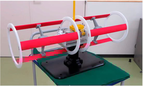
Figure 1.
Appearance prototype of the horizontal-axis H-Darrieus turbine. (Provided by Ichinomiya Denki, Co., Ltd., Hyogo, Japan).
Since the power output of WEC depends on the available wave energy, wave energy assessment is essential to the development of WECs. On a global scale, the assessment of wave energy resources has been conducted by Rusu and Rusu [8]. For example, energy density in the Atlantic Ocean can be as high as 70 kW/m. To identify suitable sites for coastal wave energy conversion, assessments have been conducted for specific marine areas [9]. Based on the above concepts, we installed the WEC in the wave-breaking zone and conducted an energy assessment there.
The power output of traditional WECs, such as oscillating water columns (OWCs) and wave-absorbing devices, is proportional to wave energy flux. In contrast, the power output of the H-Darrieus turbine is strongly influenced by the underwater flow velocity. Although energy flux is distributed nearly uniformly in the littoral zone, underwater flow velocity exhibits a complex distribution. Therefore, understanding the waves and their underwater flow in a littoral zone is important for selecting an optimal installation site and turbine conceptual design. To estimate the power output of the H-Darrieus turbine, we define wave power and conduct a detailed wave power resource assessment for a candidate area.
In this paper, we propose a semi-analytical method for evaluating coastal wave characteristics, including wave power assessment. Based on the results of the semi-analytical method, the conceptual design of the H-Darrieus turbine is determined, including the installation site, underwater velocity, turbine diameter, rotational speed, and power output. Additionally, it is desirable to have a concrete common understanding (conceptual design) in order to work in the early stages of a project or at the time of a change in direction. Therefore, the semi-analytical method is employed to evaluate coastal wave characteristics quickly and with little computational effort. The proposed method can obtain results, including visualization, for each analysis condition within one minute using one core of a typical PC, and as a result, it can be used to study various wave conditions, such as wave heights and tidal levels.
The semi-analytical method combines wave theories with simple numerical techniques to analyze the wave characteristics in the littoral zone. Airy wave theory, proposed by G. B. Airy in 1841 [10], serves as a fundamental model for describing ocean wave behavior. The linearity in the Airy theory is based on the assumption that wave heights are small relative to the water depth, allowing wave motion to be described by linear equations. In contrast, Stokes wave theory, proposed by G. G. Stokes in 1847 [11], incorporates nonlinearity and is applicable to higher wave heights. The Stokes theory accounts for the effects of higher wave heights, where the wave crest becomes sharper, and the trough flattens, capturing the asymmetry and other nonlinear behaviors of waves. Since swell waves generally have a relative wave height that is a small fraction of the water depth, approximately one-tenth or less, they are particularly suited for analysis using the Airy theory. However, steep waves right before breaking cannot be accurately calculated without incorporating nonlinearity. In this study, we employ both the Airy and Stokes theories within the semi-analytical method to analyze swell wave propagation and breaking. The semi-analytical method is well-suited for evaluating the behavior of swell waves in the littoral zone, offering a balance of theoretical simplicity, numerical feasibility, sufficient accuracy, and practical applicability. This approach serves as the foundation for the conceptual design of the horizontal-axis H-Darrieus turbine and provides a sufficient methodology.
2. The Semi-Analytical Method
A semi-analytical method evaluates the distribution of various wave characteristics in the littoral zone, including phase velocity, group velocity, wave heights, wave breaking positions, energy density, and wave power. The semi-analytical method combines the Airy and Stokes wave theories with simple numerical techniques such as the Newton–Raphson method and the Gauss–Kronrod quadrature. In the wave theories and the semi-analytical method, coastal waves, which are irregular waves, are simplified and solved as regular waves. As the proposed method does not consider wave reflection, its application to coastal areas with deep water and breakwaters requires careful consideration.
2.1. Wave Parameters
Coastal waves are specified by the following parameters: mean water depth , wave length , wave height and phase velocity as shown in Figure 2. Wave period is determined by the wave source and is constant while propagating until the wave breaks. The coastal waves are classified as the deep-water waves and the shallow-water waves, for and , respectively. Hereafter, the subscript 0 is added to the wave parameters for deep-water waves such as and .
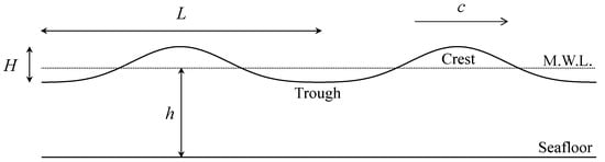
Figure 2.
Wave parameters ( is mean water depth, is wavelength, is wave height, and is phase velocity).
2.2. Dispersion Relation
According to the Airy theory, the wavenumber and angular frequency satisfy the dispersion relation:
The phase velocity (propagation speed) is given by
The group velocity (energy transfer speed) is given by
Equation (1) is accurate enough for the swell evaluation purpose, even though the dispersion relation can be refined to using the Stokes theory [12]. Since Equation (1) is an implicit equation of , it can be solved numerically using the Newton–Raphson method, and the phase velocity and group velocity are calculated from Equations (2) and (3), respectively. The phase and group velocity are normalized by the phase velocity in deep-water waves as and , respectively, and are shown in Figure 3. The relationships between the phase velocity and group velocity are in shallow-water waves and in deep-water waves, respectively. As wave shoaling progresses, the phase velocity decreases monotonically. In contrast, the group velocity shows a convex profile.
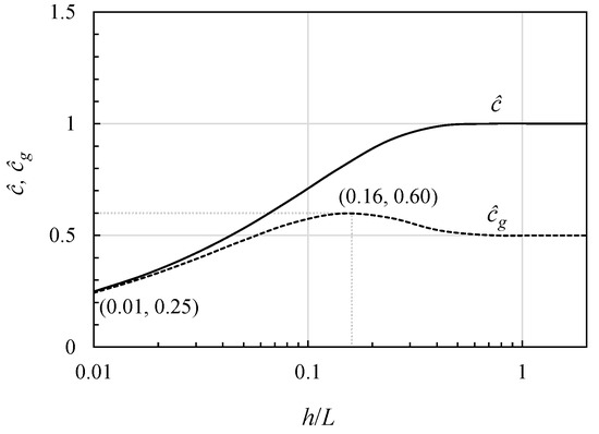
Figure 3.
Phase velocity and group velocity profiles in coastal waves.
2.3. Wave Energy and Its Conservation Property
When looking down at the ocean from the sky, the time-mean wave energy per unit area is defined as the time-mean energy density. The energy density includes the wave energy from the seafloor to the sea surface. The energy density is given by
where is the fluid density and is the gravitational acceleration. The wave energy is transferred at the group velocity in propagation, and the wave energy flux per unit crest length, also known as the energy transfer rate, is defined as
In terms of the energy conservation, the energy flux gradient in the propagating direction is given by , where is the source term. if there is an energy source such as the wave generation by the wind. if there is an energy sink, such as the wave breaking. if there are no sources or sinks of energy in wave propagation. The zero-gradient condition, , indicates that energy flux in addition to wave period , is also constant during propagation until the wave breaks. The energy flux in deep-water waves can be calculated as , and then the energy density is given by
2.4. Energy Density Profile
The group velocity is given by Equation (3), and the energy density in coastal waves can be calculated from Equation (6). The normalized energy density profile as a function of relative mean water depth is shown in Figure 4, where is the normalized energy density. The energy density in deep-water waves is given by from Equation (4), where is wave height in deep-water waves. The energy density shows a concave profile because of the convex group velocity profile; thus, there are coastal waves with less energy density.
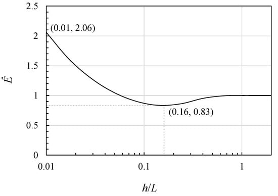
Figure 4.
Energy density profile in coastal waves.
The normalized energy density is for in deep-water waves due to its definition. During the transition from deep-water waves to shallow-water waves and also intermediate waves, the normalized energy density decays to as minimum value at . The normalized energy density is amplified to at .
2.5. Wave Height
Equations (4) and (6) yield the formula for calculating wave height:
2.6. Wave Breaking
According to Figure 4, the normalized energy density continues to increase during propagation until wave breaking actually takes place. The wave-breaking condition depends on the wave height, the wavelength, and the water depth. According to several breaking height formulas [13,14,15], the breaking height is given by
Here, represents the wave height right before breaking, and is the beach slope. The energy density profile is truncated at the point where wave breaking occurs, marking the incipient breaking position.
Equations (8a)–(8c) are derived from a theoretical–empirical approach that combines theoretical models with data obtained from field measurements. These formulas are practical due to their simplicity and because they are based solely on geometric conditions governing wave shape. Furthermore, it is generally understood that wave breaking occurs when the horizontal velocity at the peak of the wave crest exceeds the phase velocity [16]. This condition serves as an analytical breaking index in the semi-analytical method, complementing the breaking indices discussed above. Discrepancies between these breaking indices may suggest that the wave characteristics, such as phase velocity or underwater flow velocity, are not predicted with sufficient accuracy.
To calculate the coordinates of the peak at the wave crest and the corresponding horizontal velocity, the Stokes theory is employed. The coordinate at the peak of the wave crest, according to the third-order Stokes expansion, is given by: .
2.7. Underwater Flow Velocity
To evaluate breaking positions and wave power, it is important to calculate the underwater flow velocity of shallow water waves with sufficient accuracy. Using the third-order Stokes expansion, the horizontal component of the underwater flow velocity is given by the following expression:
In the above formulation, it is assumed that the dispersion relation, and , has been calculated with sufficient accuracy. We utilize the magnitude of the horizontal velocity component since it characterizes the oscillatory flow. The wave-period-averaged horizontal velocity is calculated as , which is solved analytically. The depth-and-wave-period-averaged horizontal velocity is then determined numerically using the Gauss–Kronrod quadrature method: .
2.8. Wave Power
Wave power, a fundamental concept for assessing the power output of WEC turbines, is defined as the kinetic energy across the control plane extending from the seafloor to the mean water surface. It represents the potential wave power that a turbine could extract from the wave energy in a given location. This concept is quantified by the following equation:
The wave-period-averaged calculation is solved analytically. The integration over the depth direction is then performed numerically using the Gauss–Kronrod quadrature.
The wave energy flux and wave power have the same units, Watts per unit crest length W/m, but they are proportional to different dimensions of velocity as and , respectively. At the peak of the wave crest, where the horizontal velocity is greatest, it reaches the phase velocity right before the wave breaks. In shallow-water waves, . Therefore, there is a relationship between the wave energy flux and the wave power such that .
3. Results and Discussions
An example of applying the semi-analytical method using bathymetry data obtained from multibeam sonar surveying at Seragaki, Okinawa, Japan, is shown. As illustrated in Figure 5, the Seragaki littoral zone includes several specific areas: from the offshore side, it begins with a deep zone, followed by a sharp shallowing at the drop-off topography, then transitions into the surf zone, and finally reaches the breakwater. The bathymetry data represent water depths at the mean water level, assuming no tidal variation. The coastline and breakwater at Seragaki face northward towards the sea. In the semi-analytical method, while the wave propagation direction does not explicitly appear, it is interpreted as propagating in a direction consistent with the phase velocity field. Note that the and directions represented in this section are not related to the wave propagation direction. As swell wave conditions, regular waves with the wavelength of m and the wave height of m, are assumed. In this case, the wave period is s, the phase velocity in deep-water waves is m/s, the energy density in deep-water waves is kJ/m2, and the energy flux is kW/m.
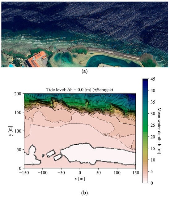
Figure 5.
Seragaki: candidate site for WEC installation: (a) aerial photo (©2024 Airbus, Maxar Technologies); (b) contour lines of mean water depth. Solid lines are shown every 5 m depth and dashed lines every 1 m depth. Seragaki is located on the north-west coast of Okinawa main island, Japan (26.513497, 127.872526).
3.1. Coastal Wave Characteristics
The phase velocity, group velocity, peak horizontal velocity, and energy density fields are shown in Figure 6, respectively. Figure 6a shows the gradual decrease in phase velocity, while Figure 6c shows the progressive increase in the peak horizontal velocity. Eventually, in the surf zone, the peak horizontal velocity exceeds the phase velocity, reaching approximately 6 m/s, at which point the wave is considered to be breaking. The energy density field, accounting for the wave height drop due to breaking, is shown in Figure 6d. For the following figures, all quantities are calculated and depicted, assuming a 60% reduction in wave height due to wave breaking. Figure 6b shows that the group velocity field increases during propagation and then decreases. In contrast, Figure 6d indicates that the energy density decreases once on the offshore side of the surf zone. Due to the sharp change in depth caused by the drop-off topography, the energy attenuation region is narrow here.
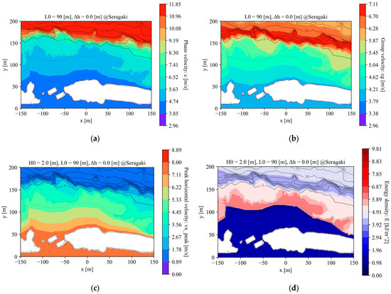
Figure 6.
Coastal wave characteristics: (a) phase velocity field; (b) group velocity field; (c) peak horizontal velocity field; (d) energy density field. In deep-water waves, the phase velocity, the group velocity, and the energy density are m/s, m/s, and kJ/m2, respectively. The peak velocity exceeds the phase velocity at approximately 6 m/s, and the incipient breaking positions are marked by sudden jumps in energy density, as indicated by the color gaps.
3.2. Wave Height and Breaking Positions
Figure 7 illustrates the wave height field, where the incipient wave-breaking positions are visible as a sudden jump in wave height, represented by a color gap in the field. The incipient breaking positions are marked by the analytical breaking index, and the results from the empirical formulas given by Equations (8a)–(8c) are indicated by the red, yellow, and blue dashed lines, respectively. To demonstrate the validity of the proposed method, the different tidal levels (Δh) and deep-water wave heights (H0) are presented in Figure A1 and Figure A2 in Appendix A, respectively.
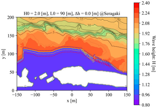
Figure 7.
Wave height field. The incipient breaking positions appear as sudden jumps in wave height, as shown in the color gap. Red, yellow, and blue dashed lines show the breaking indices using Equations (8a)–(8c), respectively.
From a mathematical perspective, even a higher-order Stokes approximation is insufficient to accurately represent shallow-water waves right before breaking [17]. Therefore, the semi-analytical solution must be validated to ensure sufficient accuracy for practical use by comparing it with empirical approaches. According to the empirical results, wave breaking occurs at the most shoreward position, as predicted by Equation (8a), at the most offshore position, as predicted by Equation (8c), and between these two positions, as predicted by Equation (8b). The acceptable agreement among these results validates the semi-analytical method, demonstrating its effectiveness in accurately predicting the breaking wave phenomenon. It is important to note that using the Airy theory or the lower-order Stokes theory to calculate peak velocity tends to underestimate the result, leading to a significant delay in predicting the incipient wave-breaking positions and a substantial underestimation of wave power.
From the perspective of conceptual turbine design, by predicting the incipient wave-breaking positions, it is possible to avoid breaking waves that cause destructive forces on WECs and to avoid post-breaking waves that contain insufficient energy. Additionally, by predicting the wave height field, it is possible to determine the trough water level and thereby establish the dimensions necessary to keep the WEC submerged.
3.3. Wave Power Field
The distribution of potential wave power for the turbine is shown in Figure 8. Since wave power is proportional to the cube of the underwater flow velocity, it changes rapidly in the surf zone due to the wave shoaling, reaching its maximum value right before the wave breaks. The maximum wave power is found in the surf zone seaward of the incipient wave-breaking positions, where the mean water depth is 3–4 m without tidal variation. The wave energy flux is kW/m, and in the region right before wave breaking, the wave power approaches a value comparable to the energy flux. Despite the small water depth in the surf zone, it contains significant wave power, making it suitable for direct energy harnessing using compact WECs. It is important to properly select the installation site, choosing areas with high wave power while avoiding both wave-breaking areas, which have destructive impacts on a WEC, and post-breaking areas, which have diminished power. The different tidal levels (Δh) and deep-water wave heights (H0) are presented in Figure A3 and Figure A4 in Appendix B, respectively.
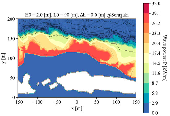
Figure 8.
Wave power field.
3.4. Conceptual Design of the H-Darrieus Turbine
In the area where maximum wave power is realized, wave shoaling leads to the development of shallow-water waves. In this area, the underwater flow follows very flat elliptical orbits because of the shallow-water waves, resulting in nearly horizontal oscillatory flow, and the depth-and-wave-period-averaged horizontal velocity is approximately 2 m/s, as shown in Figure 9.
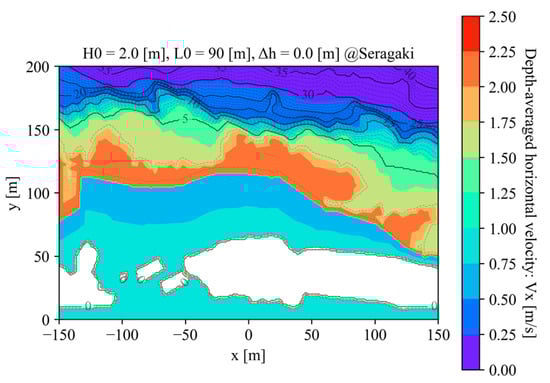
Figure 9.
Depth-and-wave-period-averaged horizontal velocity field.
To directly harness the kinetic energy from horizontal oscillatory flow, the horizontal-axis H-Darrieus turbine is a rational choice. The H-Darrieus turbine is well-suited for horizontal oscillatory flow because it continues to rotate in a constant rotational direction regardless of changes in the flow direction. In shallow-water waves, the wave propagation direction is strongly influenced by seafloor topography, causing the crestwise direction of the waves to remain parallel to the coastline. By aligning the turbine’s rotational axis with the crestwise direction of the waves, the turbine can consistently face the incoming waves, ensuring optimal power generation. Note that a vertical installation, as seen in common Darrieus wind turbines, would require a larger diameter because underwater flow speeds are significantly lower than wind speeds, potentially leading to challenges with motor speed and structural integrity.
The turbine’s power output is calculated by multiplying the potential wave power by the effective projection area and power coefficient (efficiency). The power coefficient is generally less than 0.6, a value widely recognized as the Betz limit [18]. For example, the wind power generation at 100 W/m2, assuming a turbine efficiency of 0.5 under a wind speed of 7 m/s. In our setup, to ensure the turbine remains fully submerged at a depth of 3–4 m, its diameter is restricted to approximately 2 m. Within this depth range, where the wave power is approximately 25 kW/m, a turbine with a diameter of 2 m and a mean power coefficient of 0.3 is estimated to generate a power output per unit crest length of approximately 4 kW/m. This corresponds to a power generation per unit area of 2 kW/m2. For comparison, photovoltaic power generation is estimated assuming a solar-cell efficiency of 0.2 and the solar constant. The solar constant, which is approximately 1361 W/m2 at the top of Earth’s atmosphere, is averaged across the entire surface of the Earth by considering the planet’s geometry and the day–night cycle. This results in an average solar irradiance of 340 W/m2 reaching the Earth’s surface. This leads to an annual average photovoltaic power generation of 70 W/m2. A comparison of power generation per unit area among coastal wave, wind, and photovoltaic power is shown in Table 1. For solar panels, the unit area refers to the panel’s surface area directly facing the sunlight. In contrast, for turbines, it corresponds to the effective projection area perpendicular to the dominant flow direction.

Table 1.
Comparison of power generation per unit area: coastal wave (this study), wind, and photovoltaic power.
As shown in Figure 10a, the positive torque of the H-Darrieus turbine is generated while the flow enforces upward along the blade surface in the abeam duration, producing a downward reaction force. However, if flow separates on the blade surface, the flow cannot be efficiently enforced upward, leading to a reduction in the positive torque (Figure 10b). Therefore, it is important to select an optimal combination of airfoil and TSR to prevent flow separation (Figure 10c).
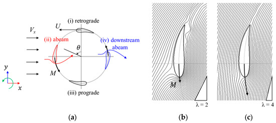
Figure 10.
Schematic of flow over an H-Darrieus turbine in a cross-sectional view: (a) Schematic of H-Darrieus turbine in the inertia frame. The colored arrows show flow pattern in the inertia frame. (b) Separating flow and (c) no flow separation visualized by streamline in the abeam state in the rotating frame, respectively. is the rotation angle, is the tip speed, is the horizontal flow velocity, and is the torque.
The variation in AoA in the blade completes one revolution, as shown in Figure 11. For conventional airfoils, flow separation tends to occur at AoA around 15 degrees; therefore, a TSR of approximately 4 is considered optimal. However, in cases where multiple blades are installed, as in typical H-Darrieus turbines, the incoming flow decelerates due to blockage effects, lowering the optimal TSR to approximately 3 [19]. For thicker airfoils, which are more resistant to flow separation, the suitable TSR decreases, while for airfoils prone to separation, a higher TSR is required.
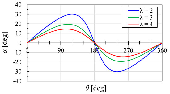
Figure 11.
The relationship of rotation angle and AoA.
Based on the discussions above, with a turbine diameter of 2 m and a TSR of 3, the turbine’s rotational speed would range from 120 to 180 rpm to maximize power. The relationship between turbine radius, rotational speed, and TSR is organized in Figure 12, assuming a maximum horizontal flow velocity of 4 m/s.
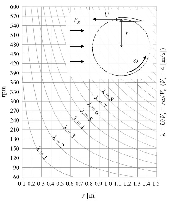
Figure 12.
The relationship between turbine radius, rotational speed (rpm), and tip speed ratio.
4. Conclusions
Details of the semi-analytical method based on the wave theories are presented in Section 2. Among them, the methods for calculating the incipient breaking positions (Section 2.6) and the wave power (Section 2.8) are extensions of the wave theories.
In Section 3, the proposed method was applied to the seabed topography and typical swell wave condition of Seragaki (Okinawa, Japan), and the wave characteristics obtained through visualization were discussed. The results for various tidal levels and wave heights, presented in Appendix A and Supplementary Materials (Video S1), validated the proposed method. As discussed in Section 3.3, the maximum wave power was approximately 25 kW/m under typical swell wave conditions at Seragaki, which was selected as the WEC installation site. In Section 3.4, the rotational mechanism of the H-Darrieus turbine is described, leading to the specific conceptual design. The water depth at the installation site is 3–4 m, limiting the turbine diameter to approximately 2 m. Given the mean horizontal flow velocity of 2 m/s, maximum horizontal velocity of 4 m/s, and TSR of 3, the estimated rotational speed was 120–180 rpm. Assuming a turbine efficiency of 30%, the power generation per unit area was evaluated as 2 kW/m2. In addition, assuming a turbine diameter of 2 m, the power generation density was evaluated as 4 kW/m. Furthermore, assuming a turbine area of 10 m2 (with an effective turbine width of 5 m), the power generation per turbine was evaluated as 20 kW.
In this study, the result under a single wave condition (a typical swell at Seragaki) was discussed in detail to outline the decision process for the conceptual design. The wave power assessment and the conceptual design for H-Darrieus WEC can be extended to account for annual and seasonal characteristics using multiple wave conditions, as shown in the Appendix A, Appendix B and Supplementary Materials. Furthermore, the proposed method can be applied to further candidate sites.
Supplementary Materials
The following supporting information can be downloaded at: https://www.mdpi.com/article/10.3390/en18061495/s1, Video S1.
Author Contributions
Conceptualization, T.S.; methodology, K.U.; software, K.U.; validation, K.U.; formal analysis, K.U.; investigation, K.U.; resources, K.U.; data curation, K.U.; writing—original draft preparation, K.U.; writing—review and editing, K.U.; visualization, K.U.; supervision, T.S.; project administration, T.S.; funding acquisition, T.S. All authors have read and agreed to the published version of the manuscript.
Funding
This research received no external funding. The APC was funded by the Institute of Computational Fluid Dynamics Co., Ltd. (iCFD).
Data Availability Statement
Source code and data created in this study are available on GitHub. (https://github.com/kazuakiuchibori/WavePowerAssessment).
Acknowledgments
The author would like to express sincere gratitude to Yu Fukunishi, Emeritus Professor at Tohoku University and Technical Advisor at the Institute of Computational Fluid Dynamics Co., Ltd. (iCFD), for his invaluable advice on fluid dynamics. His continuous guidance and kind support have been important throughout our research. The authors would like to express their sincere gratitude to the members of the wave energy converter project for their valuable collaboration, including Hideki Takebe and Jun Fujita at the Okinawa Institute of Science and Technology (OIST); Toshio Shindou and Patrick Bach at Ichinomiya Denki Co., Ltd. (IME); and Masayuki Shimizu, Hiroyasu Ochiai, Yoshiharu Yoshimura, and Takahiro Sumide at Mitsubishi Heavy Industries Machinery Systems, Ltd. (MHI-MS). During the preparation of this manuscript/study, the authors used OpenAI’s ChatGPT (GPT-4 Turbo) for English translation and coding assistance. The authors have reviewed and edited the output and take full responsibility for the content of this publication.
Conflicts of Interest
Author Kazuaki Uchibori was employed by the company Institute of Computational Fluid Dynamics Co., Ltd. The authors declare no conflicts of interest.
Appendix A. Wave Height Fields and Breaking Positions
In addition to the reference case in Section 3 (Figure 7), the wave height fields with the breaking positions for different tide levels (Δh) and deep-water wave heights (H0) are shown in Figure A1 and Figure A2, respectively. See Video S1 in the Supplementary Materials for more details.
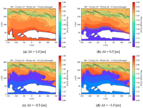
Figure A1.
Effects of tidal level (Δh) variation on wave height fields and breaking positions.
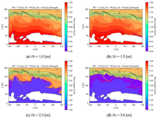
Figure A2.
Effects of wave height (H0) variation on wave height fields and breaking positions.
Appendix B. Wave Power Fields
In addition to the reference case in Section 3 (Figure 8), the wave power fields for different tide levels (Δh) and deep-water wave heights (H0) are shown in Figure A3 and Figure A4, respectively. See Video S1 in the Supplementary Materials for more details.
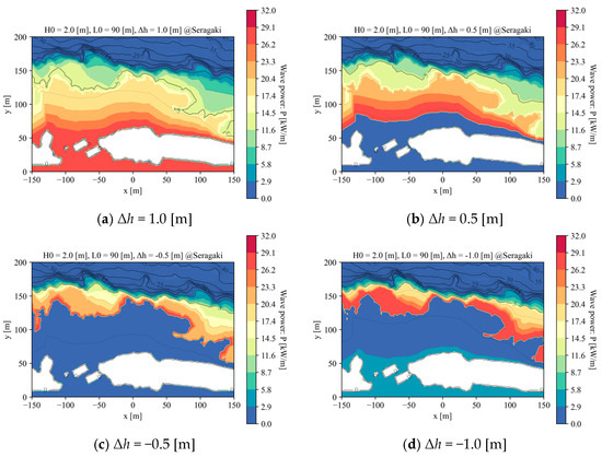
Figure A3.
Effects of tidal level (Δh) variation on wave power fields.
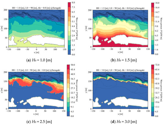
Figure A4.
Effects of wave height (H0) variation on wave power fields.
References
- Drew, B.; Plummer, A.R.; Sahinkaya, M.N. A review of wave energy converter technology. Proc. IMechE Part A J. Power Energy 2009, 223, 887–902. [Google Scholar] [CrossRef]
- List of Wave Power Projects. Available online: https://en.wikipedia.org/wiki/List_of_wave_power_projects (accessed on 18 November 2024).
- Shintake, T. Harnessing the Power of Breaking Wave. In Proceedings of the the Asian Wave & Tidal Energy Conference (AWTEC2016), Singapore, 25–27 October 2016; pp. 623–630. [Google Scholar]
- Pawitan, K.A.; Takebe, H.; Andrean, H.; Misumi, S.; Fujita, J.; Shintake, T. Duct Attachment on Improving Breaking Wave Zone Energy Extractor Device Performance. Energies 2021, 14, 6428. [Google Scholar] [CrossRef]
- Bach, P.; Shintake, T.; Takebe, H.; Fujita, J.; Shindou, T.; Uchibori, K.; Shimizu, M.; Ochiai, H.; Yoshimura, Y.; Kanno, I. Electrical Generator Design for Darrieus-Type Wave Energy Converter. J. Ocean Eng. Technol. 2025, 39, 63–72. [Google Scholar] [CrossRef]
- Du, L.; Ingram, G.; Dominy, R.G. A review of H-Darrieus wind turbine aerodynamic research. Proc. IMechE Part C J. Mech. Eng. Sci. 2019, 233, 7590–7616. [Google Scholar] [CrossRef]
- Kihoh, S.; Shiono, M. Electric Power Generations from Tidal Currents by Darrieus Turbine at Kurushima Straits. IEEJ Trans. Ind. Appl. 1992, 112, 530–538. (In Japanese) [Google Scholar] [CrossRef]
- Rusu, L.; Rusu, E. Evaluation of the Worldwide Wave Energy Distribution Based on ERA5 Data and Altimeter Measurements. Energies 2021, 14, 394. [Google Scholar] [CrossRef]
- Guillou, N.; Lavidas, G.; Chapalain, G. Wave Energy Resource Assessment for Exploitation—A Review. J. Mar. Sci. Eng. 2020, 8, 705. [Google Scholar] [CrossRef]
- Airy, G.B. Tides and waves. In Encyclopædia Metropolitana: Mixed Sciences; Smedley, E., Rose, H.J., Rose, H.J., Eds.; B. Fellowes: London, UK, 1841; Volume 3. [Google Scholar]
- Stokes, G.G. On the theory of oscillatory waves. Trans. Camb. Philos. Soc. 1847, 8, 441–455. [Google Scholar]
- Newman, J.N. Marine Hydrodynamics, 40th anniversary ed.; The MIT Press: Cambridge, MA, USA, 2017; pp. 247–263. [Google Scholar]
- Miche, R. Mouvements ondulatoires de l’océan pour une eau profonde constante et décroissante. Ann. Ponts Chaussées 1944, 114, 369–406. (In French) [Google Scholar]
- Goda, Y. Reanalysis of regular and random breaking wave statistics. Coast. Eng. J. 2010, 52, 71–106. [Google Scholar] [CrossRef]
- Fenton, J.D. Nonlinear Wave Theories. Sea Ocean. Eng. Sci. 1990, 9, 1–19. [Google Scholar]
- Goda, Y. Reanalysis of Breaking Wave Statistics for Engineering Applications. Proc. Coast. Eng. JSCE 2007, 54, 81–85. (In Japanese) [Google Scholar] [CrossRef]
- JSFM (Japan Society of Fluid Mechanics). Fluid Dynamics Handbook, 2nd ed.; Maruzen: Tokyo, Japan, 1998; pp. 661–668. (In Japanese) [Google Scholar]
- Betz, A. Introduction to the Theory of Flow Machines; Randall, D.G., Translator; Pergamon Press: Oxford, UK, 1966. [Google Scholar]
- Shiono, M.; Suzuki, K.; Kihoh, S. The experimental study on characteristics of Darrieus type turbine for the tidal power generation. IEEJ Trans. Power Energy 1998, 118, 781–787. (In Japanese) [Google Scholar]
Disclaimer/Publisher’s Note: The statements, opinions and data contained in all publications are solely those of the individual author(s) and contributor(s) and not of MDPI and/or the editor(s). MDPI and/or the editor(s) disclaim responsibility for any injury to people or property resulting from any ideas, methods, instructions or products referred to in the content. |
© 2025 by the authors. Licensee MDPI, Basel, Switzerland. This article is an open access article distributed under the terms and conditions of the Creative Commons Attribution (CC BY) license (https://creativecommons.org/licenses/by/4.0/).