A Novel Methodology for Calculating Combustion Characteristics Across the Combustion Zone Length

Abstract

This paper introduces a novel mathematical model designed to determine combustion characteristics across the length of the combustion zone, underpinned by logical theoretical foundations and demonstrating notable alignment with experimental findings. The model facilitates the calculation of combustion efficiency based on inlet flow parameters (temperature, pressure, velocity, length, porosity, and air excess ratio), achieving efficiencies beyond conventional limits (η = 0.98–0.99) and reaching high values (η = 0.999–0.9999), which is crucial for optimizing low-emission combustors. Verification of the mathematical model was conducted through a dual approach: experimental validation and computational fluid dynamics (CFD) simulations. Comparative analysis revealed a high degree of consistency among theoretical predictions, CFD results, and experimental data, particularly for temperature and combustion efficiency distributions along the combustor length. This robust agreement affirms the model’s accuracy, reliability, and utility in advancing combustion research and developing efficient, low-emission combustors.

1. Introduction

Combustion efficiency and low-emission combustors are critical to modern energy systems, including gas turbines, aerospace propulsion, and power generation [1,2,3,4]. Achieving high combustion efficiency while minimizing emissions requires precise modeling of interchamber processes such as mixture formation, ignition, and combustion [5,6,7]. However, existing approaches often lack the necessary precision or theoretical rigor, leading to suboptimal designs and extensive experimental validation [8,9]. This highlights the need for advanced methodologies that can accurately predict combustion characteristics and optimize combustor performance.

1.1. Challenges in Combustor Design

The design of efficient and low-emission combustors is a complex task that involves balancing multiple competing requirements, including operational stability, temperature uniformity, and high combustion efficiency. Traditional design methods rely heavily on empirical correlations and experimental testing, which are time-consuming and costly. Moreover, these methods often fail to account for the intricate interactions between flow dynamics, heat transfer, and chemical reactions that occur within the combustion zone [10].

One of the key challenges in combustor design is accurately predicting combustion characteristics, such as temperature, pressure, velocity, and combustion efficiency, across the length of the combustion zone. These parameters are critical for optimizing combustor performance and ensuring compliance with stringent environmental regulations. However, existing models often struggle to capture the complex physics of turbulent combustion, particularly in high-temperature and high-pressure environments.

1.2. Existing Approaches to Combustion Modeling

Current methodologies for calculating combustion characteristics can be broadly categorized into empirical, differential equation-based, and computational approaches:

• Empirical Methods: These methods rely on experimental data and correlations to predict combustion characteristics. While computationally efficient, they often lack theoretical rigor and may not account for all relevant variables, such as turbulence and chemical kinetics. For example, combustion efficiency is typically estimated using empirical equations based on emission indices, which may not fully capture the effects of turbulence, mixing, and chemical kinetics [11].
• Differential Equation-Based Methods: These models are derived from fundamental physical laws, such as the Navier–Stokes equations, and are typically solved analytically or semi-analytically. They offer greater theoretical rigor but are often limited by simplifying assumptions, such as the assumption of an infinitesimally thin combustion zone, which may not be valid for turbulent flames. For instance, Reference [12] describes a reactor-based model that cannot be derived from the Navier–Stokes equations but is still based on differential equations. These models are particularly useful for understanding the fundamental physics of combustion but may struggle to capture the full complexity of turbulent flows.
• Computational Fluid Dynamics (CFD) Simulations: CFD simulations are numerical solutions to the differential equations governing fluid flow, heat transfer, and chemical reactions. They provide detailed insights into complex flow dynamics and are widely used for combustor design and optimization [13]. However, they require significant computational resources and are often limited by the accuracy of turbulence and chemical kinetics models. For example, Reference [14] demonstrates the use of CFD simulations to model turbulent combustion, highlighting the importance of accurate turbulence modeling in capturing the behavior of turbulent flames.

Clarification on Combustion Zone Thickness:

Some models assume an infinitesimally thin combustion zone, which is a simplification that may not be valid for turbulent flames where the time-averaged combustion zone can be significant. However, it is important to note that the instantaneous combustion zone in turbulent flames can still be very thin, even though the time-averaged zone appears wide. In this study, we adopt the assumption of a thin combustion zone at the local level, which allows us to simplify the governing equations and focus on the overall behavior of the combustion process. This assumption is justified by the need to balance accuracy with computational efficiency, particularly in the context of preliminary design and optimization.

1.3. Gaps in Existing Research

Despite significant advancements in combustion modeling, several gaps remain in the accurate calculation of combustion characteristics, particularly for turbulent flames. Traditional models, such as those proposed by S. Tzyan [15], A. Scurlock [16], and F.S. Billig [17], focus primarily on laminar flames and assume an infinitesimally thin combustion zone. While these models provide valuable insights, they fail to capture the behavior of turbulent flames, where the combustion zone width is significant and cannot be neglected.

Studies by Talantov [18] have attempted to address these limitations by incorporating finite-width combustion zones and additional closure conditions. However, these approaches often diverge in their assumptions and methodologies, leading to inconsistencies in their predictions. More recent work by Mingazov [19] and Aleksandrov [20] has further advanced the field by using empirical equations to describe the increase in combustion efficiency along the length of the combustor. Their studies revealed that combustion efficiency follows a logarithmic growth pattern, increasing rapidly at first before gradually slowing down as it approaches a saturation point, but not a sigmoid-like exponential growth, where improvements occur more gradually initially but continue steadily over time, ultimately achieving higher efficiency levels. This behavior is critical for optimizing combustor design but is not fully captured by traditional models.

1.4. Novelty and Objectives of the Study

The primary objective of this study is to establish a novel mathematical model for calculating combustion characteristics with logical theoretical underpinnings and a demonstrable ability to align with the experimental findings. The proposed model addresses the limitations of existing methods by providing a robust framework for modeling turbulent flames and accurately predicting combustion efficiency and temperature distributions along the combustor length.

The key innovations of the model include the following:

• Simplified Mixture Flow Trajectories: The model divides the combustion zone into smaller regions and calculates parameters locally, allowing for precise predictions of temperature and combustion efficiency.
• Novel Combustion Efficiency Equation: The model introduces a computationally efficient and theoretically rigorous method for calculating combustion efficiency along the combustor length. This equation accounts for the logarithmic and sigmoid-like growth patterns observed in experimental studies, ensuring accurate predictions across the entire combustion zone. Specifically, it captures the rapid initial increase in efficiency as combustion initiates, followed by a gradual leveling off as the reaction approaches completion.
• Integration of Turbulence and Chemical Kinetics: The model incorporates simplified turbulence parameters and chemical kinetics to capture the complex interactions between flow dynamics and combustion processes.

2. Mathematical Model

2.1. Fundamentals and Theory

The mathematical model simplifies complexity through key assumptions. It assumes a homogeneous air–fuel mixture, treating flow as one-dimensional to streamline analysis while acknowledging real-world deviations. Velocity and temperature profiles are predefined, though actual conditions may vary. Pressure is considered constant across the chamber cross-section, ignoring localized gradients. Turbulence parameters are set in advance for computational efficiency but may not fully capture turbulent or swirling flows. While these simplifications limit accuracy in cases of non-uniform mixing or complex geometries, the model remains a useful tool for predicting combustion performance.

To accurately calculate combustion characteristics along the length of the combustion zone, the model divides the combustion chamber into several zones, each corresponding to a specific air supply configuration. Each zone is characterized by a homogeneous mixture flow with a length of (L_cz) and a height of (R_com), as illustrated in Figure 1. The combustion zone is further divided into small axial segments of length Δx and height (R_r—R_f), where the initial flow parameters are defined at the inlet of each segment with the index “o”. The outlet parameters from each segment are calculated using governing equations (Equations (1) to (8) and (39), which will be detailed in the next section). These outlet parameters then serve as the inlet conditions for the next segment, and this iterative process continues until the entire length of the combustion zone (L_cz) is covered. The same process is applied for the next layer height R_f + (R_r − R_f) (i − 1), where i is the layer number (i = 1,2,3,…).

Combustion characteristics such as velocities, temperatures, pressure, and flame front boundaries are derived using relationships in Figure 1, which provides key flow parameters essential for mathematical formulation.

The combustion characteristics within the mixing layer and flow, encompassing axial velocities of the fresh mixture w_o and combustion products w_p, temperatures of the fresh mixture T_o and combustion products T_p, pressure P, and the relative radii of the front R_f and rear R_r boundaries of the flame front, are determined using the following dependencies:

Mass conservation equation for the entire flow:

$${\rho }_{\mathrm{o}}{·W}_{\mathrm{o}}={\rho }_p{·W}_p$$

(1)

where ρ_o—the density of the fresh mixture, ρ_p—the density of combustion products.

Turbulent burning velocity:

$$u_t={\displaystyle \frac{T_p}{T_o}}·u_n+{\displaystyle \frac{A·w^{\prime }}{\sqrt{\ln \left(1+\frac{w^{\prime }}{u_n}\right)}}}$$

(2)

where u_t—turbulent flame propagation velocity [18], u_n—normal flame propagation velocity in laminar flow, A = 2.4—coefficient, pulsation speed w’ = ε w_p, ε—turbulence intensity [18].

Stagnation pressure equation:

$${{\mathrm{P}}_p}^{*}={\mathrm{P}}_p+{\displaystyle \frac{{\rho }_p{W_p}^2}{2}}$$

(3)

where ${{\mathrm{P}}_p}^{*}$—total pressure of the combustion products, ${\mathrm{P}}_p$—static pressure of the combustion products.

Stagnation temperature equation:

$${T_p}^{*}=T_p+{\displaystyle \frac{{W_p}^2}{2{\mathrm{C}}_{\mathrm{p}}}}$$

(4)

where ${T_p}^{*}$—total temperature of the combustion products, $T_p$—static temperature of the combustion products, C_p—specific heat capacity.

Combustion product velocity:

$$W_p={\displaystyle \frac{∆x}{{\tau }_p}}$$

(5)

where ${\tau }_p$—time required for the combustion product to travel distance Δx, as shown in Figure 1.

Trigonometric functions:

$$\sin \alpha ={\displaystyle \frac{u_t}{W_{\mathrm{o}}}}$$

(6)

$$\tan \alpha ={\displaystyle \frac{R_r-R_f}{∆x}}$$

(7)

Combustion temperature determined from the heat balance (energy equation):

$${T_p}^{*}\left(\mathrm{x}\right)=T_o+{\displaystyle \frac{H_u·{\eta }_{\mathrm{x}}}{{Cp}_i·\left(1+{\propto }_o·L_o\right)}}$$

(8)

where H_u—calorific value of fuel, η_x—combustion efficiency, L_o—the stoichiometric ratio, α_o—excess air coefficient, ${Cp}_i$—specific heat capacity

2.2. Combustion Efficiency

To determine the combustion efficiency along the combustion length, following Ya.B. Zeldovich [21], flame propagation is the consequence of heat transfer from the burning gas to the unburned mixture. The equation of thermal conductivity for gases wherein combustion occurs is derived. Thermal conductivity is analyzed for various temperature, reaction rate, and fuel concentration scenarios along the x coordinate, which can be schematically represented by the graph in Figure 2.

The thermal conductivity equation for any point within the combustion zone can be derived by considering the boundary conditions at the extremes of the curve.

We establish the initial conditions on the left side (x = −∞), where w = 0, T = T_o, and m = m_o. Similarly, on the right side (x = +∞), where w = 0, T = T_p, and m = 0, we define the conditions at the end of the curve.

Taking these boundary conditions into account, the equation of thermal conductivity can be formulated as follows:

$${\mathrm{C}}_{\mathrm{p}}\rho {\displaystyle \frac{\partial \mathrm{T}}{\partial t}}=-{\rho u\mathrm{C}}_{\mathrm{p}}{\displaystyle \frac{\partial \mathrm{T}}{\partial x}}+\lambda {\displaystyle \frac{{\partial }^{2}T}{\partial x^2}}+\varphi (T,m)$$

(9)

where ${\mathrm{C}}_{\mathrm{p}}\rho {\displaystyle \frac{\partial \mathrm{T}}{\partial t}}$ represents the change in the amount of heat per unit of volume per unit of time, ${\displaystyle \frac{\partial \mathrm{T}}{\partial t}}$ represents the rate of 103 change in temperature concerning time, and λ—represents the thermal conductivity coefficient, which characterizes the ability of the material to conduct heat.

The equation for heat generated by a chemical reaction is represented as

$$\varphi \left(T,m\right)=Qw$$

(10)

where Q is the heat effect per one mole of the reaction, and w is the reaction rate.

For steady-state combustion, after replacing partial derivatives with total derivatives, Equation (9) can be expressed as follows:

$${u\rho \mathrm{C}}_{\mathrm{p}}{\displaystyle \frac{d\mathrm{T}}{dx}}={\displaystyle \frac{d}{dx}}\left(\lambda {\displaystyle \frac{dT}{dx}}\right)+\varphi (T,m)$$

(11)

where uρ represents the gas mass passing through a unit of cross-section per unit of time, which remains constant due to the law of conservation of matter. When integrating the equation,

$$u\rho =const={\left(\rho u\right)}_{T_o}=u_n{\rho }_o$$

(12)

Several approximate methods have been proposed to circumvent the complexities of integrating Equation (11), such as the Jouguet–Daniell method [22]. This method assumes that the function Φ changes with temperature according to a step law, as illustrated in Figure 3. Specifically, at temperatures below T_i and above T_p, Φ = 0, and within the range T_i ≤ T ≤ T_p, Φ remains constant.

At the same time, assuming that the thermal conductivity coefficient λ does not vary with temperature, Equation (11) allows for the temperature to be divided into two distinct regions:

In region I, where T_o ≤ T ≤ T_i, referring to Figure 3:

$${\rho u\mathrm{C}}_{\mathrm{p}}{\displaystyle \frac{d\mathrm{T}}{dx}}=\lambda {\displaystyle \frac{d^{2}T}{d{x}^2}}$$

(13)

And in region II, where T_i ≤ T ≤ T_p, referring to Figure 3:

$${u\rho \mathrm{C}}_{\mathrm{p}}{\displaystyle \frac{\partial \mathrm{T}}{\partial x}}=\lambda {\displaystyle \frac{d^{2}T}{d{x}^2}}+\varphi$$

(14)

Having established the origin in the (T, x) system at the point corresponding to the boundary between regions I and II at T = T_i, we derive from Equations (13) and (14)

$${\mathrm{T}}_{\mathrm{I}}={\mathrm{T}}_{\mathrm{o}}+({\mathrm{T}}_i-{\mathrm{T}}_{\mathrm{o}})·e^{{\displaystyle \frac{{u\rho \mathrm{C}}_{\mathrm{p}}}{\lambda }}x}$$

(15)

$${\mathrm{T}}_{\mathrm{I}\mathrm{I}}=B_1{e}^{{\displaystyle \frac{{u\rho \mathrm{C}}_{\mathrm{p}}}{\lambda }}x}+B_2+{\displaystyle \frac{\varphi }{{u\rho \mathrm{C}}_{\mathrm{p}}}}x$$

(16)

Furthermore, the equation for T_II is applicable only for the values 0 ≤ x ≤ x_p, as illustrated in Figure 2.

The boundary conditions for the obtained solutions can be expressed as follows:

x = 0: T_I = T_II and ${\displaystyle \frac{d{\mathrm{T}}_{\mathrm{I}}}{dx}}={\displaystyle \frac{d{\mathrm{T}}_{\mathrm{I}\mathrm{I}}}{dx}}$;

x = x_p: T_II = T_p and ${\displaystyle \frac{d{\mathrm{T}}_{\mathrm{I}\mathrm{I}}}{dx}}=0$.

Substituting the boundary conditions into Equations (15) and (16), we derive four equations:

$$B_1+B_2={\mathrm{T}}_i$$

(17)

$${\displaystyle \frac{\varphi }{{u\rho \mathrm{C}}_{\mathrm{p}}}}+{\displaystyle \frac{{u\rho \mathrm{C}}_{\mathrm{p}}}{\lambda }}{B}_1={\displaystyle \frac{{u\rho \mathrm{C}}_{\mathrm{p}}}{\lambda }}({\mathrm{T}}_i-{\mathrm{T}}_{\mathrm{o}})$$

(18)

$${\mathrm{T}}_{\mathrm{p}}={\displaystyle \frac{\varphi }{{u\rho \mathrm{C}}_{\mathrm{p}}}}{x}_p+B_2+B_1{e}^{{\displaystyle \frac{{u\rho \mathrm{C}}_{\mathrm{p}}}{\lambda }}{x}_p}$$

(19)

$${\displaystyle \frac{\varphi }{{u\rho \mathrm{C}}_{\mathrm{p}}}}+{\displaystyle \frac{{u\rho \mathrm{C}}_{\mathrm{p}}}{\lambda }}{B}_1{e}^{{\displaystyle \frac{{u\rho \mathrm{C}}_{\mathrm{p}}}{\lambda }}{x}_p}=0$$

(20)

Substituting $B_2={\mathrm{T}}_i-B_1$ and $B_1={\displaystyle \frac{\varphi \lambda }{{\left({u\rho \mathrm{C}}_{\mathrm{p}}\right)}^2}}{e}^{-{\displaystyle \frac{{u\rho \mathrm{C}}_{\mathrm{p}}}{\lambda }}{x}_p}$ from Equation (20) into Equation (19), we obtain

$${\displaystyle \frac{\varphi }{{u\rho \mathrm{C}}_{\mathrm{p}}}}{x}_p-{\displaystyle \frac{\varphi \lambda }{{\left({u\rho \mathrm{C}}_{\mathrm{p}}\right)}^2}}\left({1-e}^{{\displaystyle \frac{{u\rho \mathrm{C}}_{\mathrm{p}}}{\lambda }}{x}_p}\right)={\mathrm{T}}_{\mathrm{p}}-{\mathrm{T}}_i$$

(21)

Since it follows from the energy balance equation that

$${u\rho \mathrm{C}}_{\mathrm{p}}\left({\mathrm{T}}_{\mathrm{p}}-{\mathrm{T}}_{\mathrm{o}}\right)=\varphi ·x_p$$

(22)

then, to determine u, we obtain the transcendental equation:

$${\mathrm{T}}_i-{\mathrm{T}}_{\mathrm{o}}-{\displaystyle \frac{\varphi \lambda }{{\left({u\rho \mathrm{C}}_{\mathrm{p}}\right)}^2}}\left({1-e}^{-{\displaystyle \frac{{{(u\rho \mathrm{C}}_{\mathrm{p}})}^2\left({\mathrm{T}}_{\mathrm{p}}-{\mathrm{T}}_{\mathrm{o}}\right)}{\lambda \varphi }}}\right)=0$$

(23)

Denoting ${\displaystyle \frac{{{(u\rho \mathrm{C}}_{\mathrm{p}})}^2\left({\mathrm{T}}_{\mathrm{p}}-{\mathrm{T}}_{\mathrm{o}}\right)}{\lambda \varphi }}={\mathrm{y}}^2$ and ${\displaystyle \frac{{\mathrm{T}}_i-{\mathrm{T}}_{\mathrm{o}}}{{\mathrm{T}}_{\mathrm{p}}-{\mathrm{T}}_{\mathrm{o}}}}=\mathrm{a}$, we finally find

$${\displaystyle \frac{{1-e}^{-{\mathrm{y}}^2}}{{\mathrm{y}}^2}}=\mathrm{a}$$

(24)

u is defined as follows:

$$u=\mathrm{y}\sqrt{{\displaystyle \frac{\varphi \lambda }{{\left({\rho \mathrm{C}}_{\mathrm{p}}\right)}^2({\mathrm{T}}_{\mathrm{p}}-{\mathrm{T}}_{\mathrm{o}})}}}$$

(25)

We introduce a reaction time t_r, which is defined as the time it takes to release all the heat per unit volume at a constant rate Φ:

$$t_r·\varphi ={\rho \mathrm{C}}_{\mathrm{p}}\left({\mathrm{T}}_{\mathrm{p}}-{\mathrm{T}}_{\mathrm{o}}\right)$$

(26)

and then Equation (25) is transformed into

$$u=\mathrm{y}\sqrt{{\displaystyle \frac{\lambda }{{\rho \mathrm{C}}_{\mathrm{p}}}}{\displaystyle \frac{1}{t_r}}}$$

(27)

For x < 0, the temperature depends on x according to the following law:

$$\mathrm{T}={\mathrm{T}}_{\mathrm{o}}+({\mathrm{T}}_i-{\mathrm{T}}_{\mathrm{o}})·e^{{\displaystyle \frac{{u\rho \mathrm{C}}_{\mathrm{p}}}{\lambda }}x}$$

(28)

At 0 ≤ x ≤ x_p, combustion occurs, and at x ≥ x_p, the temperature is equal to T_p. Also, for x < 0, Expression (28) is valid, leading to

$${\displaystyle \frac{d\mathrm{T}}{dx}}=\left({\mathrm{T}}_i-{\mathrm{T}}_{\mathrm{o}}\right)·{\displaystyle \frac{{u\rho \mathrm{C}}_{\mathrm{p}}}{\lambda }}·e^{{\displaystyle \frac{{u\rho \mathrm{C}}_{\mathrm{p}}}{\lambda }}x}$$

(29)

and for x = 0, this expression is converted to

$${\left({\displaystyle \frac{d\mathrm{T}}{dx}}\right)}_{x\to 0-0}=({\mathrm{T}}_{\mathrm{i}}-{\mathrm{T}}_{\mathrm{o}})·{\displaystyle \frac{{u\rho \mathrm{C}}_{\mathrm{p}}}{\lambda }}$$

(30)

For x > x_p, T = T_p = const. and ${\displaystyle \frac{d\mathrm{T}}{dx}}=0$.

Lev Abramovich Vulis made a significant contribution to the field of combustion dynamics by proposing an expression for determining the combustion efficiency along the combustor length [23]. This formula, which is crucial for understanding thermal dynamics in combustion systems, was later adopted and applied in further studies, including those by V.P. Savchenko [24]. The expression is as follows:

$$\eta (\mathrm{x})={\displaystyle \frac{1}{1+\frac{1}{{\overline{\tau }}_{rn}}+\frac{1}{{\overline{\tau }}_{rd}}}}$$

(31)

where ${\overline{\tau }}_{rn}={\displaystyle \frac{{\tau }_r}{{\tau }_n}}$, ${\overline{\tau }}_{rd}={\displaystyle \frac{{\tau }_r}{{\tau }_d}}$—the ratio of the residence time of the combustion mixture in the combustor τ_r, respectively, to the characteristic reaction time τ_n and to the time of turbulent diffusion τ_d.

When the reaction time (τ_n) is significantly shorter than the residence time (τ_r), which implies that τ_n is much less than τ_r (τ_n << τ_r), the ratio τ_r/τ_n approaches zero (${\displaystyle \frac{{\tau }_n}{{\tau }_r}}\approx 0$).

In this case, from Equation (31), we can simplify the expression, leading to

$$\eta (\mathrm{x})\cong {\displaystyle \frac{1}{1+\frac{{\tau }_d}{{\tau }_r}}}$$

(32)

From the conservation equations:

$$m{H}_u+{\mathrm{C}}_{\mathrm{p}}T=m_o{H}_u+{\mathrm{C}}_{\mathrm{p}}{T}_o={\mathrm{C}}_{\mathrm{p}}{T}_p$$

(33)

Transforming the equation, we arrive at

$${\displaystyle \frac{m}{m_o}}={\displaystyle \frac{T_p-\mathrm{T}}{T_p-T_o}}$$

(34)

From the molecular diffusion equation, we have

$$d\mathrm{M}=-D_T{\displaystyle \frac{dc}{dx}}dFd{\tau }_d$$

(35)

where D_T—the molecular diffusion coefficient [m²/s], dc/dx—concentration gradient in the direction of diffusion [kg/m³], dF—cross-sectional surface area through which a stream flows [m²], dτ_d—time [s], and dM—amount of diffused substance [kg m].

In this equation, all parameters (D_T, dc/dm, dF) are constants, allowing us to write

$${\tau }_d=m_{\mathrm{o}}\left(1-{\displaystyle \frac{m}{m_{\mathrm{o}}}}\right)·const$$

(36)

Substituting Equation (34) into (36), we obtain

$${\tau }_d={\displaystyle \frac{\mathrm{T}-{\mathrm{T}}_{\mathrm{o}}}{{\mathrm{T}}_{\mathrm{p}}-{\mathrm{T}}_{\mathrm{o}}}}·const$$

(37)

and from Equation (28), we obtain

$${\displaystyle \frac{T-T_o}{T_i-T_o}}=e^{{\displaystyle \frac{{u\rho \mathrm{C}}_{\mathrm{p}}}{\lambda }}x}$$

(38)

Substituting Equations (38) and (37) into (32), we obtain

$$\eta \left(\mathrm{x}\right)\cong {\displaystyle \frac{1}{1+e^{\mathrm{a}\overline{x}+b}}}$$

(39)

where $\overline{x}={\displaystyle \frac{\mathrm{x}}{L_{req}}}$, and $L_{req}=B{\displaystyle \frac{l_o}{\epsilon }}\ln \left(1+{\displaystyle \frac{w^{\prime }}{u_n}}\right)$—required the combustion zone length for fuel burnout; B—constant [18]; $\epsilon ={\displaystyle \frac{w^{\prime }}{v_{av}}}$—turbulence intensity; v_av—mean dimensionless flow velocity in the zone [18]; $l_o=2l_{mix}$—Eulerian turbulence scale [18]; l_mix—Lagrangian scale of turbulence; $b=\mathrm{l}\mathrm{n}\left(\mathrm{c}\mathrm{o}\mathrm{n}\mathrm{s}\mathrm{t}\right)$—constant; a—constant; λ—effective turbulent thermal conductivity, ${\tau }_r={\displaystyle \frac{V{\rho }_p}{G_p}}$, where V is the volume in each section, ρ_p is the density of combustion products, and G_p is the mass flow rate of combustion products.

3. Validation of the Mathematical Model

The testing of the developed mathematical model was conducted through experimental validation and computational fluid dynamics (CFD) simulations. This dual approach enabled a comprehensive comparison of predicted combustion characteristics against actual measurements, ensuring model accuracy and robustness.

3.1. Experimental Setup

The experimental validation was conducted in a modular combustion chamber designed to simulate and measure the combustion process under various conditions (Figure 4).

The facility included the following:

• Air Supply System: Equipped with a main blower (32 kW, 200 kW) and an auxiliary blower (2.2 kW), along with ducts, bypasses, and throttle valves to regulate airflow. The air was heated to 180 °C using a heat exchanger and a closed-loop air heating system to prevent contamination of combustion products (Figure 5).
• Fuel Supply System: Consisting of propane/butane, natural gas, and CO₂ containers, gas reducers, isolation valves, mixers, and nozzles. Precise fuel regulation was ensured through gas reducers and stopcocks.
• Measurement System: Included a calibrated orifice plate for air flow measurement, thermocouples for temperature monitoring, and a gas analyzer (Polar-T) for gas composition analysis. Sampling was performed via a two-tube system: one cooled for “frozen” gas samples and another heated to 700–800 K to prevent condensation.

The combustion efficiency was determined using a gas analysis system, which involved sampling through two separate tubes (Figure 6 illustrates the measurement system setup). One tube was cooled with water to rapidly halt the chemical reaction in the sample, allowing for the collection of a “frozen” gas sample. Before reaching the gas analyzer, this sample was directed through a three-way valve, a refrigerator, and a desiccant. Simultaneously, another tube was maintained under a voltage of 27 V to heat it to a temperature of 700–800 K, preventing condensation. This heated sample was sent through an afterburner within an electric furnace and then to the gas analyzer. Tungsten–rhenium thermocouples (TVR-6) were employed for accurate combustion temperature measurement.

The combustion efficiency is calculated as follows:

$$\eta ={\displaystyle \frac{\overline{C{O}_2}+0.5\overline{CO}}{C{O}_2^{*}}}$$

(40)

where $C{O}_2^{*}$—the percentage content of carbon dioxide in the afterburned samples, $\overline{C{O}_2}$ and $\overline{CO}$—the percentage content of $C{O}_2$ and $CO$ in the quenched sample, respectively.

3.2. Working Regime for the Nodular Combustor

To ensure consistency between experimental and computational studies, the boundary conditions were maintained as shown in

Table 1. Boundary conditions for the modular combustor.

Boundary	Value
Air inlet mass flow rate	0.034 kg/s
Air inlet temperature	353 K
Air inlet pressure	1.1 × 105 Pa
Air excess ratio α	2.5

.

3.3. Computational Fluid Dynamics Simulations for the Modular Combustor

CFD simulations were performed to complement experimental validation and provide a detailed understanding of combustion dynamics. The process involved the following:

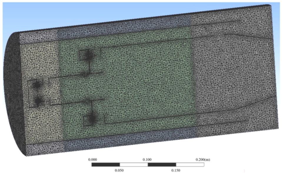
• Geometric and Meshing Details: In the CFD simulations of the combustion chamber, the geometric model was constructed using NX software NX 10.0 and meshed in ANSYS, ANSYS 19R1 yielding approximately 2.5 million tetrahedral elements (Figure 7). The mesh generation process incorporated various refinements to capture intricate flow dynamics accurately, especially near the walls and critical geometric regions.

The key parameters included a maximum element size of 5.0 × 10⁻³ m and a minimum edge length of 1.9572 × 10⁻⁴ m, with curvature capturing enabled to improve mesh resolution in curved areas. Proximity and defeature size settings were adjusted to preserve small geometric details essential for combustion modeling. The average surface area of the mesh elements was 3.2311 × 10⁻³ m, with a bounding box diagonal of 0.32232 m. Mesh quality checks confirmed a maximum skewness of 0.83, ensuring that numerical errors from poor element shapes were minimized (Figure 8).

A grid independence study was conducted to assess the impact of mesh density on simulation accuracy (Figure 9). Five meshes were tested: Grid A (1.5 million elements), Grid B (2.5 million), Grid C (3.5 million), Grid D (4.5 million), and Grid E (5.5 million). Identical boundary conditions were applied across all cases. The results indicated a marginal variation in the computed average outlet temperature: a 4.1% change between Grids A and B, but only a 0.49% variation between Grids B and C. This demonstrated that beyond 3.5 million elements, the solution converged with negligible improvement in accuracy. Consequently, Grid B was selected as the optimal mesh for numerical simulations, achieving a balance between computational cost and result fidelity.

This detailed meshing approach, with high resolution near boundaries and refined skewness thresholds, ensures robust flow characterization, enhancing the predictive capability of the CFD model.

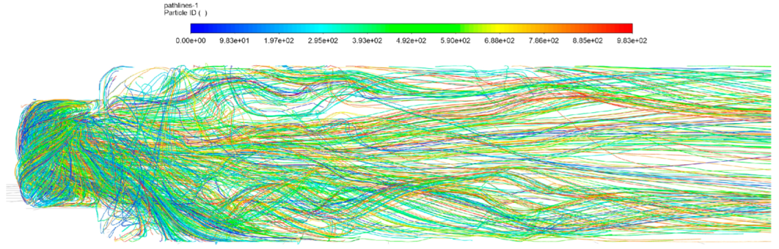
• Simulation Approach: The CFD simulations were carried out using ANSYS Fluent 19R1 to analyze the fluid flow characteristics. The simulations employed the Reynolds-averaged Navier–Stokes (RANS) equations, which are commonly used for modeling turbulent flows. Specifically, the k-ε RNG turbulence model was chosen due to its proven reliability in combustion simulations. This model accounts for the effects of turbulence in various fluid dynamic scenarios and has been widely applied in similar contexts. To accurately model the chemical reactions involved in the combustion process, the Kee chemical kinetics mechanism was implemented. This mechanism, widely used in combustion modeling, provides a detailed representation of reaction pathways and species interactions, enhancing the predictive capabilities of the simulation. Additionally, to ensure the accuracy and consistency of the simulations, identical boundary conditions to the experimental setup were applied, as referenced in previous studies [25,26].
• Convergence and Averaging: Simulations ran for ~10,000 iterations, with results averaged over the last 2000 iterations to account for steady-state behavior.

3.4. Results and Comparison for the Modular Combustor

To process the obtained results, special control surfaces were employed at the same locations where measurements were taken during the experiments. The average mass parameters per unit cross-sectional area were calculated at each control surface.

The combustion efficiency was calculated using the following formula [27]:

$$\eta =1-{\displaystyle \frac{\dot{m_C}}{\dot{m_{C\left(in\right)}}}}$$

(41)

where ${\dot{m}}_C$ is the average mass concentration of carbon (in all forms), and ${\dot{m}}_{C\left(in\right)}$ is the average mass concentration of carbon in the fuel inlet.

The temperature distribution along the combustor length, obtained from CFD simulations, closely matched both experimental and theoretical data (see Figure 10). The maximum deviation observed between the CFD and experimental temperatures was 8.12%, while the difference between the quasi-one-dimensional calculation and experimental data was 9.05%. These small discrepancies are within acceptable limits, further affirming the accuracy of the mathematical model.

Similarly, the comparison of combustion efficiency along the combustor length, presented in Figure 11, showed that CFD simulations predicted values within 12.3% of the experimental measurements and 11.03% within the theoretical model predictions of the experimental measurements. This close agreement demonstrates that the CFD model accurately captures the combustion process and validates the combustion efficiency derived from the mathematical model.

The incorporation of CFD modeling enhances the analysis by offering detailed visualizations, such as the temperature distribution along the combustion chamber (Figure 12). These insights reveal a high-temperature region near the wall, suggesting the necessity to extend the premixed zone for improved performance. However, this observation does not undermine the efficacy of the proposed model. Despite its relative simplicity, the model accurately predicts critical combustion outcomes, including the completion of combustion and the achievement of a uniform temperature distribution at the chamber’s exit, as demonstrated in Figure 12. This indicates that while CFD modeling provides a more granular view, the proposed model remains effective in capturing essential combustion characteristics.

Velocity magnitude contours (Figure 13) further illustrate the flow dynamics, emphasizing the role of inlet flow parameters in shaping the internal flow structure. The velocity field indicates a steady acceleration downstream, with minimal backflow or turbulence-induced inefficiencies. This confirms the model’s robustness in predicting flow uniformity and combustion efficiency, as the observed velocity profiles correspond closely with experimental benchmarks.

Particle pathlines (Figure 14) depict detailed flow trajectories and reveal the interaction between fuel–air mixing and combustion propagation. The pathlines show a highly streamlined flow with minimal recirculation zones, contributing to efficient mixing and reduced unburnt fuel zones. These visualizations underscore the model’s ability to capture key dynamics and validate its performance in designing combustors that achieve optimal combustion with minimal emissions.

The comparative analysis of theoretical predictions, CFD simulations, and experimental data reveals a satisfactory correlation. The quasi-one-dimensional mathematical model, despite its simplicity, accurately predicts critical outcomes, including the completion of combustion and uniform exit temperature profiles. The CFD visualizations add a deeper understanding of the combustion dynamics, illustrating the impact of flow parameters on performance. This combination of theoretical and computational methods reinforces the model’s applicability for designing efficient, low-emission combustors.

4. Validation of the Mathematical Model for the Second Design

To further verify the validity and generalizability of the proposed mathematical model, it was tested on a second combustor design. This additional validation increases the reliability of the model and demonstrates its applicability to different combustion chamber configurations. The same test rig, as shown in Figure 5, was utilized for this purpose, ensuring consistency in experimental conditions.

The second design tested is a two-zone tubular reverse-flow combustor. This combustor consists of two distinct zones: a pilot zone and a main zone, each equipped with its own fuel manifold and swirler for flame stabilization and efficient mixing of the air–fuel mixture. The geometric 3D model of the combustor is shown in Figure 15.

4.1. Working Regime for the Two-Zone Combustor

To ensure consistency between experimental and computational studies, the boundary conditions were maintained as shown in

Table 2. The boundary conditions for the two-zone combustor.

Boundary	Case 1	Case 2	Case 3	Case 4	Case 5	Case 6
Air inlet mass flow rate, g/s	266.6	263.6	269.5	205.9	218.3	225.5
Fuel inlet mass flow rate, g/s	5.9	4.2	3.66	4.4	3.3	3.2
Air inlet temperature, K	277	277	277	423	423	423

. Six different cases were tested, varying the air inlet mass flow rate, fuel inlet mass flow rate, and air inlet temperature.

4.2. Computational Fluid Dynamics Simulations for the Two-Zone Combustor

The CFD simulations for the second combustor design were conducted using a mesh model composed of ~5 million tetrahedral elements. Wall layers and mesh condensation were applied in areas with complex geometries to ensure accurate resolution of flow dynamics. The mesh quality was maintained with a maximum skewness of 0.83, as shown in Figure 16.

The simulation approach and convergence criteria were consistent with those used for the first combustor design. The Reynolds-averaged Navier–Stokes (RANS) equations were solved using the k-ε RNG turbulence model, and the Kee chemical kinetics mechanism was employed to model the combustion process. Simulations were run for approximately 10,000 iterations, with results averaged over the last 2000 iterations to ensure steady-state behavior.

4.3. Results and Comparison for the Two-Zone Combustor

The results of the CFD simulations were compared with experimental data for the two-zone combustor. Figure 17 shows the comparison of calculated and experimental temperatures at the outlet section for two different air inlet temperatures (277 K and 423 K). The experimental data points are represented by solid (●) and hollow (○) circles, respectively.

The results demonstrate a strong agreement between the CFD predictions and experimental measurements, with deviations within 8% for temperature distributions. This close alignment further validates the accuracy and reliability of the mathematical model for different combustor designs and operating conditions.

Additionally, a systematic underestimation of the calculated data relative to the experimental data was observed. This discrepancy arises due to the specific settings of the calculation model used to determine these values. However, due attention was not given to this issue since the deviation was well below the permissible limits set by combustion standards. The primary objective of this study was to validate the proposed methodology rather than to achieve an exact numerical match, and the results effectively demonstrate its reliability in modeling complex combustion phenomena.

5. Conclusions

This study presents a novel mathematical model for calculating combustion characteristics, validated across two distinct combustor designs. The model demonstrates high predictive accuracy and computational efficiency, making it a valuable tool for optimizing combustion systems. Below, we summarize the key findings and contributions of this work:

• Validation of the Mathematical Model: The mathematical model was validated against experimental data for two different burner designs: a single-zone combustion burner and a two-zone tubular combustion burner operating in reverse flow. In both cases, the model showed reasonable predictive accuracy, with temperature distributions and predicted combustion efficiencies deviating by less than 15% from experimental measurements. This divergence may be attributed to simplifications in the model, which certainly increase accuracy with their reduction but also increase complexity.
• Validation Across Multiple Burner Designs: The model was rigorously validated on two distinct burner designs, each with unique geometric and operational characteristics. This validation demonstrates the quality of the model and its simplicity of use. However, in more complex combustion chambers, the model faces challenges in accurately dividing the combustion zones according to the direction of flow.
• Novelty of the Combustion Efficiency Equation: The model introduces a computationally efficient and theoretically rigorous method for calculating combustion efficiency along the burner. This method exhibits a sigmoid-like exponential growth behavior, reflecting the physical reality of combustion efficiency increasing rapidly at first as the reaction initiates and then leveling off as the reaction approaches completion. This behavior captures the gradual improvement in combustion efficiency observed in experiments, providing a more accurate representation of the combustion process.
• Comparison with Other Methods: It must be acknowledged that there are more accurate calculation methods than the proposed model, such as CFD and others. However, these methods are often more expensive, labor-intensive, and complex. The proposed model, in contrast, offers a computationally efficient and user-friendly alternative, providing quick insights for the preliminary design and optimization of combustion systems. While automation in CFD methods accelerates data acquisition, it can inadvertently distance researchers from the underlying physical phenomena. In contrast, the proposed method emphasizes active user engagement with computational methods, fostering a stronger comprehension of the underlying principles and ensuring robust and innovative outcomes.

In future work, we plan to extend the model’s validation to more complex geometries, such as annular and can-type combustors, and explore its performance under transient conditions using URANS or LES models. Specific improvements will include incorporating more detailed turbulence models, extending the model to higher dimensions to better capture complex flow features, and addressing the limitations of the quasi-1D approximation. These efforts will enhance the model’s applicability to a broader range of combustion systems and operating conditions.

References

1. Liu, Y.; Sun, X.; Sethi, V.; Nalianda, D.; Li, Y.G.; Wang, L. Review of modern low emissions combustion technologies for aero gas turbine engines. Prog. Aerosp. Sci. 2017, 94, 12–45. [Google Scholar] [CrossRef]
2. Guellouh, N.; Szamosi, Z.; Siménfalvi, Z. Combustors with low emission levels for aero gas turbine engines. Int. J. Eng. Manag. Sci. 2019, 4, 503–514. [Google Scholar] [CrossRef]
3. Zhao, Q.; Gao, Y.; Liu, C.; Mu, Y.; Xu, G.; Zhu, J. Experimental investigation into the effect of main stage swirl on flow and spray characteristics inside a stratified partially premixed combustor. Proc. Inst. Mech. Eng. Part A J. Power Energy 2023, 237, 765–776. [Google Scholar] [CrossRef]
4. Ju, H.; Zhou, R.; Zhang, D.; Deng, P.; Wang, Z. Effects of Oxygen Concentration on Soot Formation in Ethylene and Ethane Fuel Laminar Diffusion Flames. Energies 2024, 17, 3866. [Google Scholar] [CrossRef]
5. Huang, T.; Ren, X.; Chen, Y.; Ma, J.; Yi, D.; Wan, Z.; Yu, B.; Zeng, W. Transient Combustion Characteristics of Methane–Hydrogen Mixtures in Porous Media Burner. ACS Omega 2024, 9, 19525–19535. [Google Scholar] [CrossRef] [PubMed]
6. Kiss, A.; Szabó, B.; Kun, K.; Weltsch, Z. Prediction of Efficiency, Performance, and Emissions Based on a Validated Simulation Model in Hydrogen–Gasoline Dual-Fuel Internal Combustion Engines. Energies 2024, 17, 5680. [Google Scholar] [CrossRef]
7. Parente, A.; de Joannon, M. MILD Combustion: Modelling Challenges, Experimental Configurations, and Diagnostic Tools. Front. Mech. Eng. 2021, 7, 726633. [Google Scholar] [CrossRef]
8. Orlik, E.V.; Starov, A.V.; Shumsky, V.V. Determination of burnout completeness in a combustion model by the gas-dynamic method. Combust. Explos. Phys. 2004, 40, 23–34. (In Russian) [Google Scholar]
9. Baklanov, A.V. Development of the two-fuel combustion chamber and calculation of processes for the theory of turbulent burning. Sib. Aerosp. J. 2024, 25, 372–383. [Google Scholar] [CrossRef]
10. Lefebvre, A.H.; Ballal, D.R. Gas Turbine Combustion: Alternative Fuels and Emissions; CRC Press: Boca Raton, FL, USA, 2010. [Google Scholar]
11. Şöhret, Y.; Kıncay, O.; Karakoç, T.H. Combustion efficiency analysis and key emission parameters of a turboprop engine at various loads. J. Energy Inst. 2015, 88, 490–499. [Google Scholar] [CrossRef]
12. Sychenkov, V.A.; Baklanov, A.V.; Yousef, W.M. Calculation of Parameters for Combustor with the Air–Fuel Mixture Premixing. Russ. Aeronaut. 2021, 64, 277–282. [Google Scholar] [CrossRef]
13. Mishra, N. Efficient Solvers for Nonlinear Partial Differential Equations in Computational Fluid Dynamics. Adv. Nonlinear Var. Inequalities 2023, 26, 76–93. [Google Scholar] [CrossRef]
14. Li, Y.; Li, R.; Li, D.; Bao, J.; Zhang, P. Combustion characteristics of a slotted swirl combustor: An experimental test and numerical validation. Int. Commun. Heat Mass Transf. 2015, 66, 140–147. [Google Scholar] [CrossRef]
15. Tzyan, S. Aerodynamics of rarefied gases. In Gas Dynamics; Publishing House of the Academy of Sciences: Kyiv, Ukraine, 1950. [Google Scholar]
16. Scurlock, A.C. Flame Stabilization Studies; M.I.T. Progress Report; Massachusetts Institute of Technology: Cambridge, MA, USA, 1947. [Google Scholar]
17. Billig, F.S. Diffusion Flames; McGraw-Hill: New York, NY, USA, 1950. [Google Scholar]
18. Talantov, A.V. Basics of calculating the simplest direct-flow combustion chamber. Izv. VUZ. Aviats. Tekh. 1958, 3, 95–104. (In Russian) [Google Scholar]
19. Mingazov, B.G.; Aleksandrov, Y.B.; Kosterin, A.V.; Tokmovtsev, Y.V. Combustion Processes and Automated Design of Combustion Chambers of Gas Turbine Engines and Gas Turbine Plants; Manual; Publishing House of KNITU-KAI: Kazan, Russia, 2015. (In Russian) [Google Scholar]
20. Aleksandrov, Y.B.; Mingazov, B.G. Determination of completeness of combustion, temperature and emission characteristics in a swirl flow based on the theory of turbulent combustion. Vestn. Samara Univ. Aerosp. Mech. Eng. 2024, 23, 123–136. [Google Scholar] [CrossRef]
21. Zeldovich, Y.B. Selected Works of Yakov Borisovich Zeldovich, Volume I: Chemical Physics and Hydrodynamics; Section 19: A Theory of Thermal Flame Propagation; Princeton University Press: Princeton, NJ, USA, 2014; Volume 140, pp. 262–270. [Google Scholar]
22. Williams, F.A. Combustion Theory; CRC Press: Boca Raton, FL, USA, 2018. [Google Scholar]
23. Vulis, L.A. Thermal Regimes of Combustion; Russian Edition—1954; McGraw-Hill: New York, NY, USA, 1961. [Google Scholar]
24. Savchenko, V.P. Generalization of the experience of organizing turbulent combustion in combustion chambers of aerospace and power-generating engines. Bull. Samara State Aerosp. Univ. 2002, 2, 97–111. (In Russian) [Google Scholar]
25. Sabirzyanov, A.N.; Yavkin, V.B.; Aleksandrov, Y.B.; Markushin, A.N.; Baklanov, A.V. Modeling of emission characteristics of gas turbine engine combustion chambers. In Problems and Prospects of Development of Aviation, Land Transport and Energy “ANTE-2013”, Proceedings of the VII International Scientific and Technical Conference, Samara, Russia, 15–17 May 2013; Samara State Aerospace University: Samara, Russia, 2013; Volume 1, p. 355. [Google Scholar]
26. Sabirzyanov, A.N.; Yavkin, V.B.; Aleksandrov, Y.B.; Markushin, A.N.; Baklanov, A.V. Emission characteristics and temperature non-uniformity at the exit from the gas turbine combustion chamber. Bull. Samara State Aerosp. Univ. Named After Acad. S. P. Korolev 2013, 41, 165–172. Available online: https://cyberleninka.ru/article/n/emissionnye-harakteristiki-i-temperaturnaya-neravnomernost-na-vyhode-iz-kamery-sgoraniya-gtu/viewer (accessed on 1 January 2020).
27. Gerlinger, P.; Stoll, P.; Kindler, M.; Schneider, F.; Aigner, M. Numerical investigation of mixing and combustion enhancement in supersonic combustors by strut induced streamwise vorticity. Aerosp. Sci. Technol. 2008, 12, 159–168. [Google Scholar] [CrossRef]
Figure 1. Schematic diagram of flowing stream calculation. Rcom—radius of the combustor, Rr—radius of the front edges of the flame front, Rf—radius of the rear edges of the flame front, Δx—axial distance over which the velocity change occurs, α—inclination angle of the velocity vector, lcz—length of combustion zone.
Energies 18 01470 g001
Figure 2. Transition from the initial state to the final state, where p is the combustion zone width.
Energies 18 01470 g002
Figure 3. Change in function Φ with temperature according to the step law.
Energies 18 01470 g003
Figure 4. Schematic of the modular combustor.
Energies 18 01470 g004
Figure 5. Schematic of the experimental test rig facility. 1—main blower, 2—throttle valve, 3—heat exchanger, 4—measuring device, 5—thermocouple group Chromel-Copel (type L), 6—test combustor, 7—pressure gauge, 8—stopcocks, 9—gas reducer, 10—LPG bottle for main combustor, 11—gas sampling and temperature measurement site.
Energies 18 01470 g005
Figure 6. Sketch of the measurement system: Sampling is conducted via tube “A”, which directs the flow to a cooled tube for “frozen” gas samples, and via tube “B”, which directs the flow to a heated tube.
Energies 18 01470 g006
Figure 7. Geometric 3D model of the modular combustor.
Energies 18 01470 g007
Figure 8. Computational grid through the axis of the modular combustor.
Energies 18 01470 g008
Figure 9. Grid independence study.
Energies 18 01470 g009
Figure 10. Comparison of calculated, experimental, and CFD values of gas temperature along the combustor length.
Energies 18 01470 g010
Figure 11. Comparison of calculated, experimental, and CFD values of combustion efficiency along the combustor length.
Energies 18 01470 g011
Figure 12. Static temperature (K) in the plane passing through the combustion chamber centerline.
Energies 18 01470 g012
Figure 13. Velocity magnitude (m/s) distribution across the combustion chamber.
Energies 18 01470 g013
Figure 14. Particle pathlines illustrating flow trajectories within the combustion chamber.
Energies 18 01470 g014
Figure 15. Geometric 3D model of the two-zone combustor. 1—pilot zone; 2—main zone; 3—outlet section (mixing zone); 4—pilot zone fuel manifold; 5—fuel supply holes; 6—double tangential vane swirler; 7—liner of radial holes; 8—main zone fuel manifold, 9—fuel supply holes; 10—double tangential vane swirler with counter-twist; 11—liner of radial holes of the mixing zone.
Energies 18 01470 g015
Figure 16. Computational grid through the axis of the two-zone combustor.
Energies 18 01470 g016
Figure 17. Comparison of the calculated and experimental data for gas temperature and excess air coefficient at the outlet section for different inlet temperatures: ●—experiment at an air inlet temperature of 277 K; ○—experiment at an air inlet temperature of 423 K.
Energies 18 01470 g017