The Effect of Walls on the Sky View Factors of Photovoltaic Systems

Abstract

Photovoltaic collectors deployed in multiple rows and near the structure’s walls are obscured from the receiving part of the diffuse skylight. Obscuring part of the diffuse skylight to the collectors decreases the incident diffuse radiation and thus, results in diffuse radiation losses. These losses are associated with the sky view factors. The inter-row diffuse radiation losses are associated with the sky view factor of the collector, and the wall diffuse radiation losses are associated with the sky view factor caused by the wall. The purpose of the present study is to develop mathematical expressions and a methodology for sky view factors of PV systems installed near obscuring walls. The study investigates the effect of the wall height, distance of the wall to the collectors, and collector and wall azimuth angles, on the sky view factors. The study may assist the PV system designer in assessing the contribution of the incident diffuse radiation to the generated electric energy of PV systems installed near obscuring walls. The simulation results indicate that the overall range of the sky view factor variation may be quite noticeable, between 0.97 (without the presence of a wall) and 0.78 (with the presence of a wall), for the parameters used in the study.

1. Introduction

The diffuse solar radiation may comprise a significant portion of the global solar radiation in many locations and hence, the incident diffuse radiation on photovoltaic (PV) collectors may play an important role on the generated electric energy. A PV collector row (or collector), in the present study, comprises several PV modules mounted on a frame of given dimensions and inclined with an inclination angle with respect to a horizontal plane. A PV system comprises several collector rows installed behind each other. The incident diffuse radiation on PV collectors is coupled to the sky view factor, $V{F}^C$, whether using an isotropic or an anisotropic diffuse radiation model. For isotropic skies, for example, the incident diffuse radiation $G_d$ is given by $G_d=V{F}^C\times G_{dh}$, where $G_{dh}$ is the diffuse radiation on a horizontal surface, i.e., the relation between the incident diffuse radiation on a given surface and the horizontal diffuse radiation, $G_{dh}$, which is the value of the sky view factor. The sky view factor indicates the part of the sky for diffuse radiation that is visible to the PV collectors. This part depends on the nearby obscuring objects, for example, rows of collectors in a solar field mounted in front of the collector, structures, trees, and others. Since only a part of the sky is visible to the PV collector, the sky view factor of the collector $V{F}^C<1.0$; therefore, the collector receives less diffuse solar radiation by the factor $(1-V{F}^C)$. The energy loss of the diffuse radiation part is termed “masking losses”. In addition, PV systems suffer from shading losses stemming from direct beam radiation. Wall and inter-row shading losses are investigated in [1]. The present article focuses on masking losses.

View factors to the sky and to grounds of flat surfaces were widely published in the literature.

The sky view factor (SVF) for collectors mounted in multiple rows on horizontal and inclined planes was first investigated in [2]. The articles in [3,4,5] deal with the view factors to the sky, to the ground and between collectors, deployed in multiple rows. A catalogue of different view factors is in [6]. Sky view factors for collectors mounted on rooftops are reported in [7]. The work in [8] analyzes the SVF for isotropic and anisotropic diffuse and albedo radiation. The calculation of the SVF using the Monte Carlo method is presented in [9], and the SVF calculation using the finite element method is in [10]. Sky view factors for the front and the rear sides of bifacial PV modules are determined by using the cross-string rule by Hottel [11] in [12]. A different approach to determining the SVF is in [13], deriving from simulated fisheye images.

Many studies deal with the analysis and sizing of PV systems considering the SVF of the collectors. These studies deal with PV systems deployed in open spaces, i.e., at locations without obscuring objects. Some studies mention obscuring objects like wires, chimneys on rooftops, trees, and others. However, these studies are concerned with the detrimental effect of the objects’ shading on the I-V characteristics and means to minimize the shading losses. The deployment of solar PV systems on rooftops in urban areas may suffer from both shading and masking by the surrounding building walls. The expressions for the sky view factors of PV systems installed near obscuring walls were not developed, or at least not published in the literature, to the best of our knowledge. As the penetration of PV systems has significantly increased from rural spaces to built environment areas, the visible sky to the systems becomes more limited by building walls and as a result, reducing the generated electric energy. The motivation of the present study is therefore to develop mathematical expressions for the sky view factors of PV systems installed near obscuring walls, and to investigate the system parameters affecting the sky view factors. The mathematical expressions and methodology presented in this article may assist the PV system designer in assessing the contribution of the incident diffuse radiation component to the generated electric energy. The present article may also inspire future investigation of PV systems installed in urban areas and on grounds near ridges. The parameters affecting the sky view factors include wall height, distance of walls to the collectors, collector length, and collector and wall azimuth angles.

2. Methods and Materials

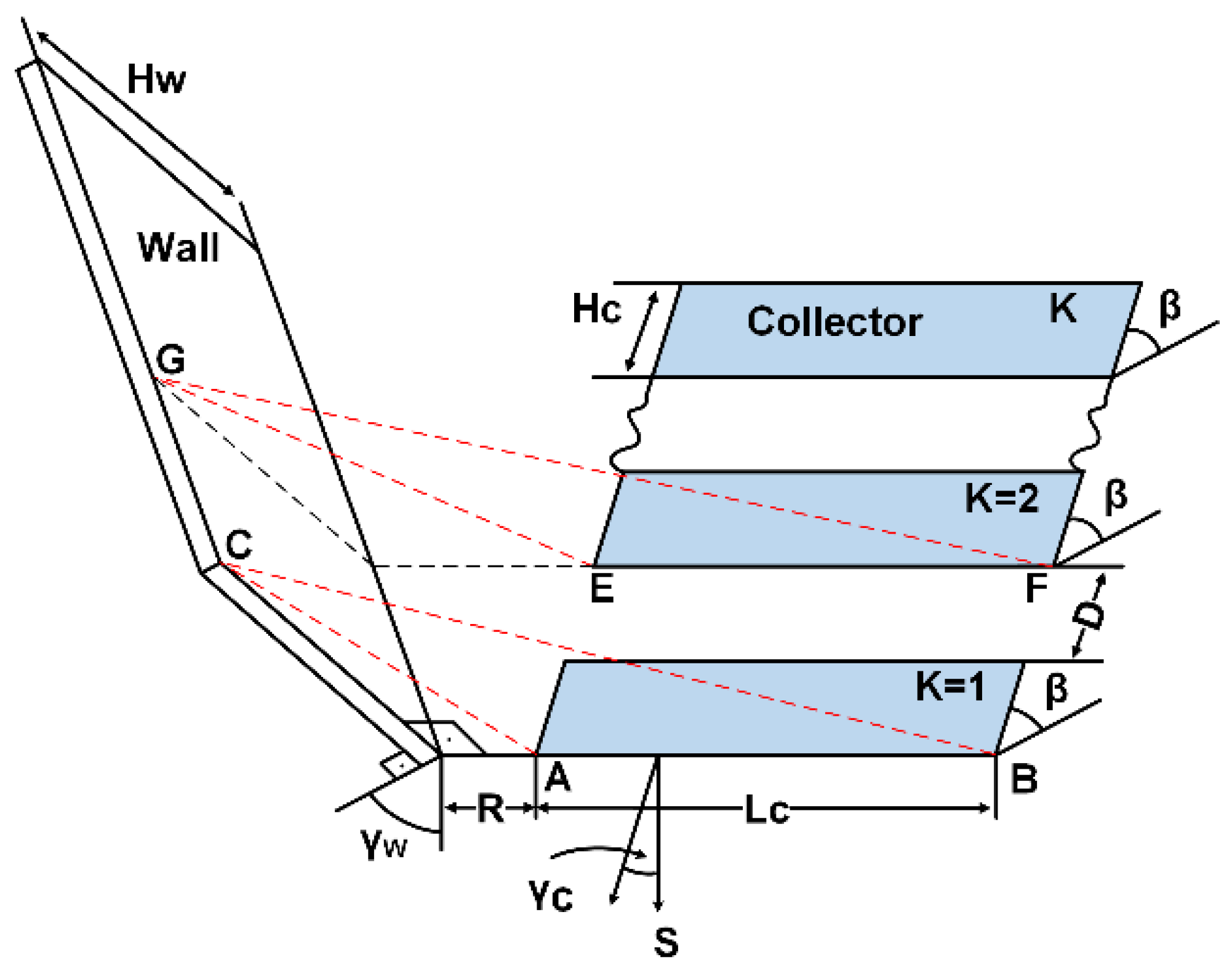
Figure 1 describes a deployment of photovoltaic (PV) collectors in a solar field on a horizontal plane in the presence of a vertical wall of a building. The collectors are of length $L_C$ and width $H_C$, deployed in east–west direction and facing in a southern direction with an azimuth angle ${\gamma }_C$ with respect to the south, inclined with an angle $\beta$ with respect to the horizontal plane, and separated by an inter-row spacing $D$. A wall of heigth $H_W$ is erected at the west side of the solar field in a south–north direction at a distance $R$ from the first collector, and oriented with an azimuth angle ${\gamma }_W$ with respect to the south. The length of the solar field, comprising $K$ collectors is given by $K\times H_C\times \cos \beta +(K-1)\times D$, see Figure 1. The length of the solar fields is longer than the dimensions of the collectors’ length and width, justifying the use of Hottel’s “cross-string rule” [11] for the calculation of the incident diffuse radiation on the collector (the cross-string rule is widely used in the literature for multiple collector rows). As the diffuse radiation arrives from all parts of the sky dome, the collectors may receive an additional part of the diffuse radiation arriving from the surrounding edges of the wall, for a wall length shorter than the solar field length. The incident diffuse radiation on a horizontal plane, in the presence of a wall, is given by $G_d^h=V{F}_R^h\times G_{dh}$, where $V{F}_R^h$ is the SVF of a horizontal plane in the presence of a wall. In general, collectors in open space receive diffuse radiation depending on the inter-row SVF, $V{F}^C$; therefore, the incident diffuse radiation on a collector in the presence of a wall, $G_C^W$, becomes

$$G_C^W=V{F}^C\times G_d^h=V{F}^C\times V{F}_R^h\times G_{dh}=V{F}^{comb.}{G}_{dh}$$

(1)

i.e., the combined SVF of a collector $V{F}^{comb.}$ comprises the SVF caused by the wall with respect to a horizontal plane $V{F}_R^h$ and the inter-row SVF of the collector $V{F}^C$.

Using the isotropic diffuse radiation model, the variation of the combined SVF of a collector represents also the variation of the incident diffuse radiation on that collector. The isotropic diffuse radiation model is used throughout the article.

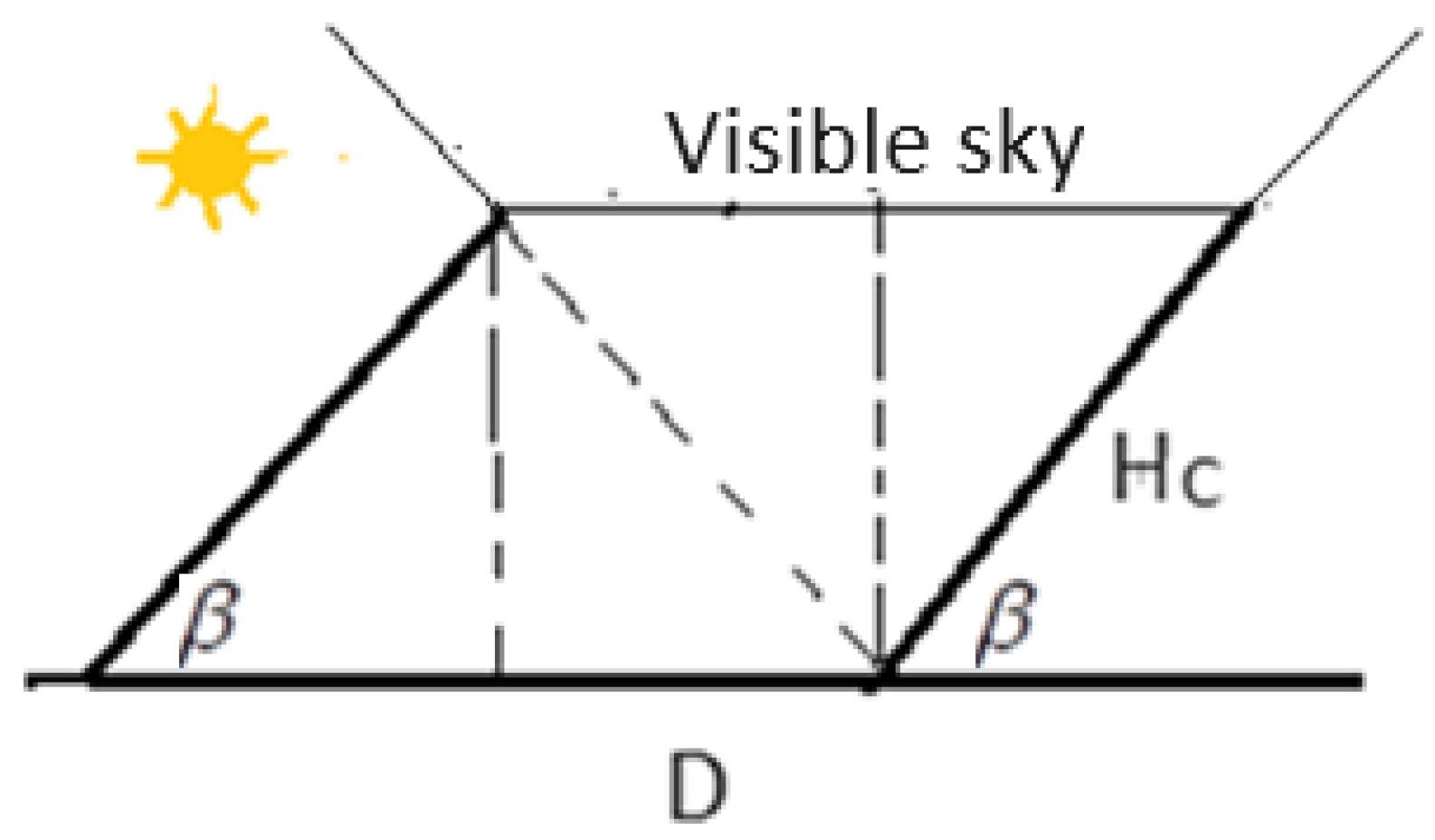
The SVF of a horizontal plane to the sky, in the presence of a wall of height $H_W$ at a distance $R$, is given, see Figure 2, by $V{F}_R^h={\displaystyle \frac{AB+BC-AC}{2\times AB}}$ [11]; therefore, the SVF of a horizontal plane of length $L_C$ at a distance $R$ from the wall, for the first collector $K=1$, see Figure 1, is as follows:

$$V{F}_R^h={\displaystyle \frac{L_C+BC-AC}{2\times L_C}}$$

(2)

and for the second collector $K=2$ (see Figure 1) is given by the following:

$$V{F}_R^h={\displaystyle \frac{L_C+FG-EG}{2\times L_C}}$$

(3)

The Liu–Jordan method [14] for the anisotropic diffuse radiation model applies to single collectors. The SVF of the first collector (see Figure 1) using the method is as follows:

$$V{F}^C=(1+\cos \beta )/2$$

(4)

The inter-row SVF of the second and the subsequent rows are determined based on the “cross-string rule by Hottel”, [11], see Figure 3:

$$V{F}^C={\displaystyle \frac{H_C+D+H_C\cos \beta -{[D^2+{(H_C\sin \beta )}^2]}^{1/2}}{2\times H_C}}$$

(5)

The combined SVF, Equation (1), of the collector is thus as follows:

$$V{F}^{conb.}=V{F}^C\times V{F}_R^h$$

(6)

2.1. General Deployment of PV Collectors near a Wall

A general deployment of PV collectors in the vicinity of a wall is shown in Figure 4, where the azimuth of the collectors and the wall are ${\gamma }_C$ and ${\gamma }_W$, respectively. The combined SVF, $V{F}^{comb.}$, depends on the distance $R$ between the wall and the collector, see Figure 4, hence a general expression is now developed for the distance $R(K)$ between the wall and the collectors. The angle $\sphericalangle ACO=90°-{\gamma }_W$ and the angle $\sphericalangle BAO=\sphericalangle ACO+{\gamma }_C=90°-{\gamma }_W+{\gamma }_C$, hence $AO={\displaystyle \frac{R(1)}{\tan (90°-{\gamma }_W+{\gamma }_C)}}$, $R(2)=[AO+(H_C\times \cos \beta +D)]\times \tan (90°-{\gamma }_W+{\gamma }_C)$, finally results in the following:

$$R(2)=R(1)+(H_C\times \cos \beta +D)\times \tan (90°-{\gamma }_W+{\gamma }_C)$$

(7)

and hence,

$$R(K)=R(1)+(K-1)(H_C\times \cos \beta +D)\times \tan (90°-{\gamma }_W+{\gamma }_C)$$

(8)

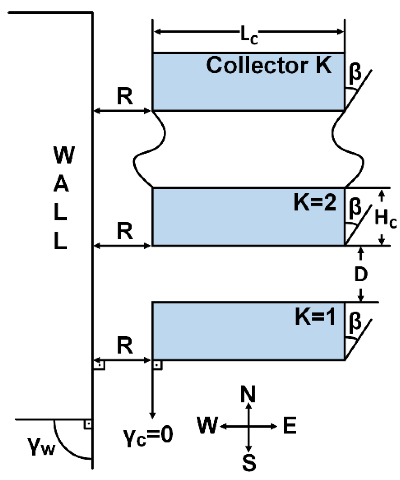
2.2. A Deployment of PV Collectors ${\gamma }_C=0°$ and a Wall ${\gamma }_W=90°$

A deployment of collectors in the east–west direction ${\gamma }_C=0°$, and a vertical wall in the north–south direction, ${\gamma }_W=90°$, is shawn in Figure 5.

The sky view factors $V{F}^C$ of the first collector, and the second and the subsequent collectors are given in Equations (4) and (5), respectively. The combined SVF, $V{F}^{conb.}$, is given in Equation (6). The SVF of a horizontal plane $V{F}_R^h$ in the presence of a wall of height $H_W$, is given in Equation (2), resulting in the following (see Figure 1):

$$V{F}_R^h={\displaystyle \frac{L_C+BC-AC}{2\times L_C}}={\displaystyle \frac{L_C+{[H_W^2+{(R+L_C)}^2]}^{1/2}-{[H_W^2+R^2]}^{1/2}}{2\times L_C}}$$

(9)

For $H_W>>L_C$ and $H_W>>R$, $V{F}_R^h$$\to 1/2$, a value known for a semi-surface.

For $H_W=0$, $V{F}_R^h=1$, a value known for a horizontal surface.

The SVF in Equation (9) applies to all collectors in the field.

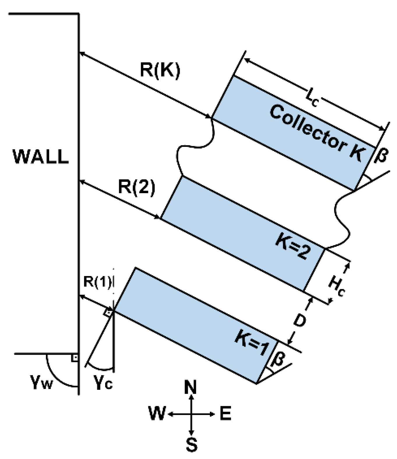
2.3. A Deployment of PV Collectors ${\gamma }_C\ne 0°$ and a Wall ${\gamma }_W=90°$

Collectors deployed in the east–west direction with an azimuth angle ${\gamma }_C\ne 0$ and a vertical wall of height $H_W$ in the north–south direction, ${\gamma }_W=90°$, is shawn in Figure 6.

The sky view factors $V{F}^C$ of the first collector, and the second and the subsequent collectors are given in Equations (4) and (5), respectively. The combined SVF, $V{F}^{conb.}$, is given in Equation (6).

The SVF, $V{F}_R^h$, of the horizontal plane for the collector $K$ at a distance $R(K)$, see Figure 6, is as follows:

$$V{F}_R^h={\displaystyle \frac{L_C+{\left\{{[L_C+R(K)]}^2+H_W^2\right\}}^{1/2}-[{(R{(K)}^2+H_W^2]}^{1/2}}{2\times L_C}}$$

(10)

where $R(K)$ is given in Equation (8).

2.4. A Deployment of PV Collectors ${\gamma }_C=0°$ and a Wall ${\gamma }_W\ne 90°$

Collectors deployed in the east–west direction ${\gamma }_C=0°$ and a vertical wall of height $H_W$ in the north–south direction with an azimuth angle ${\gamma }_W$, is shawn in Figure 7.

Based on Equation (8) for ${\gamma }_C=0°$, the distance $R(K)$ (see Figure 7) between the collector $K$ and the wall is given by the following:

$$R(K)=R(1)+(K-1){\displaystyle \frac{H_C\cos \beta +D}{\tan {\gamma }_W}}$$

(11)

The sky view factors $V{F}^C$ of the first collector, and the second and the subsequent collectors are given in Equations (4) and (5), respectively. The combined SVF, $V{F}^{conb.}$, is given in Equation (6). The SVF, $V{F}_R^h$, of the horizontal plane for the collector $K$ is given in Equation (10), where $R(K)$ is given in Equation (11).

2.5. A Deployment of PV Collectors ${\gamma }_C=-30°$ and a Wall ${\gamma }_W=30°$

Collectors deployed in the east–west direction with an angle ${\gamma }_C=-30°$ and a vertical wall of height $H_W$ in the north–south direction with an angle ${\gamma }_W=30°$ with respect to the south (the collectors are parallel to the vertical wall), is shawn in Figure 8.

Based on Equation (8) for ${\gamma }_C=30°$, the distance $R (K)$ between the collector $K$ and the wall is given by the following:

$$R(K)=R(1)+(K-1)(H_C\cos \beta +D)\tan 30°$$

(12)

The sky view factors $V{F}^C$ of the first collector, and the second and the subsequent collectors are given in Equations (4) and (5), respectively. The combined SVF, $V{F}^{conb.}$, is given in Equation (6). The SVF, $V{F}_R^h$, of the horizontal plane for the collector $K$ is given in Equation (10), where $R(K)$ is given in Equation (12).

3. Results

The percentage of incident diffuse radiation on a collector deployed near an obscuring wall is calculated by the difference between the amount of the annual incident diffuse radiation on the second collector (and subsequent collectors) in the absence of a wall, and the amount of the annual incident diffuse radiation on a collector in the presence of a wall, relative to the annual incident diffuse radiation on a collector in absence of a wall:

$$\mathrm{\Delta }{G}_d^c(\%)=100\times {\displaystyle \frac{V{F}^C{G}_{dh}-V{F}^{comb.}{G}_{dh}}{V{F}^C{G}_{dh}}}=100\times {\displaystyle \frac{V{F}^C-V{F}^{comb.}}{V{F}^C}}$$

(13)

see Equations (4)–(6).

The sky view factors of PV systems contain nine parameters-$L_C, H_C, D, \beta , K, H_W, R, {\gamma }_C, {\gamma }_W$. Three of the parameters $H_C, \beta , D$ are assumed constant values, and the rest are variable parameters of the study. The width of the PV module $H_C$ corresponds to a module with 72 cells, and with its frame, the collector width is 2.12 m. The assumed inclination angle $\beta =20°$ relates to systems site, and the inter-row spacing $D$ is the result of $H_C$ and $\beta$ values.

3.1. View Factor to Horizontal Plane, See Figure 5

Figure 9 depicts the variation of the SVF, Equation (9), of a horizontal plane $V{F}_R^h$ as a function of the collector length $L_C$ for the distance $R=2 \mathrm{m}$ between the collectors and the wall, and for wall height $H_W=1,2,3,4 \mathrm{m}$. The figure indicates that the SVF increases for longer collectors $L_C$ and for lower wall heights, $H_W$. The SVF is more evident for shorter collectors.

Figure 10 shows the variation of the SVF, $V{F}_R^h$, (Equation (9)) as a function of the distance $R$, collector length $L_C=20 \mathrm{m}$ and wall height, $H_W=1,2,3,4 \mathrm{m}$. The figure indicates that $V{F}_R^h$ decreases for shorter distances of the collector to the wall, and for higher walls.

The SVF of the first collector, Equation (4), for an inclination angle of the collector $\beta =20°$, is 0.97. The inter-row SVF, Equation (5), of the second and the subsequent rows, is 0.917 for parameters $D=1.05 \mathrm{m},H_C=2.12 \mathrm{m},\beta =20°$, i.e., a noticeable difference. The inter-row SVF value of the second collector is of about the same order of magnitude as compared to the SVF of a horizontal plane caused by a wall, especially for shorter collectors and for shorter distances of the collector to the wall, see Figure 9 and Figure 10.

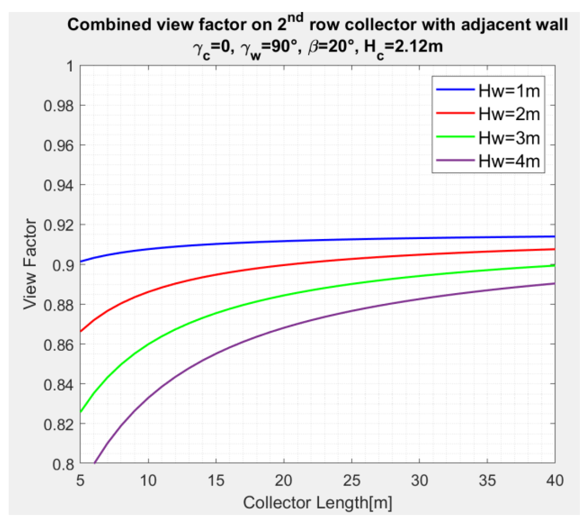
Figure 11 and Figure 12 depict the variation of the combined (wall and inter-row) sky view factors $V{F}^{conb.}$ of the first and the second collector, respectively, as a function of the collector length $L_C$, distance $R=2 \mathrm{m}$, and wall height, $H_W=1,2,3,4 \mathrm{m}$. The calculations are based on Equations (4), (6) and (9), and for $H_C=2.12 \mathrm{m},\beta =20°,D=1.05 \mathrm{m}$.

By comparing Figure 11 and Figure 12, one may notice the appreciable effect of the inter-row SVF of the second collector (Equation (5)) compared to the SVF of the first collector (Equation (4)).

Figure 13 shows the variation of the combined SVF, $V{F}^{conb.}$, of the second and subsequent collector rows, as a function of the distance $R$ from the wall for $H_C=2.12 \mathrm{m},\beta =20°,D=1.05 \mathrm{m}$, $L_C=20 \mathrm{m}$ and wall height $H_W=1,2,3,4 \mathrm{m}$, see Equations (5), (6) and (9). The combined SVF increases and levels off to larger view factors as the distances of the collector to the wall increase.

3.2. Combined View Factors, See Figure 6

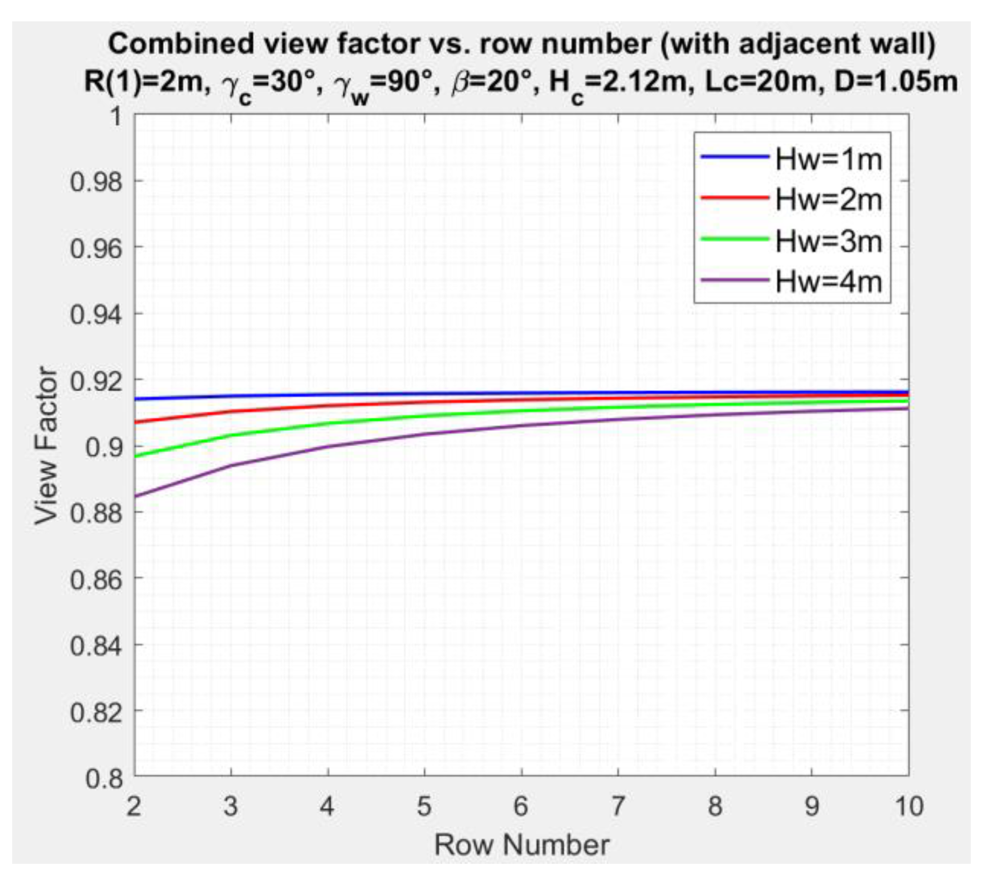
Figure 14 depicts the variation of the combined SVF, $V{F}^{comb.}$, of the second collector, as a function of the collector number $K$, for distance $R(1)=2 \mathrm{m}$, collector azimuth angle ${\gamma }_C=30°$, and wall height $H_W=1,2,3,4 \mathrm{m}$. The calculations are based on Equations (5), (6), (8) and (10), and for $H_C=2.12 \mathrm{m},\beta =20°,D=1.05 \mathrm{m},L_C=20 \mathrm{m}$. The Figure shows a small variation of the SVF with the collector row number.

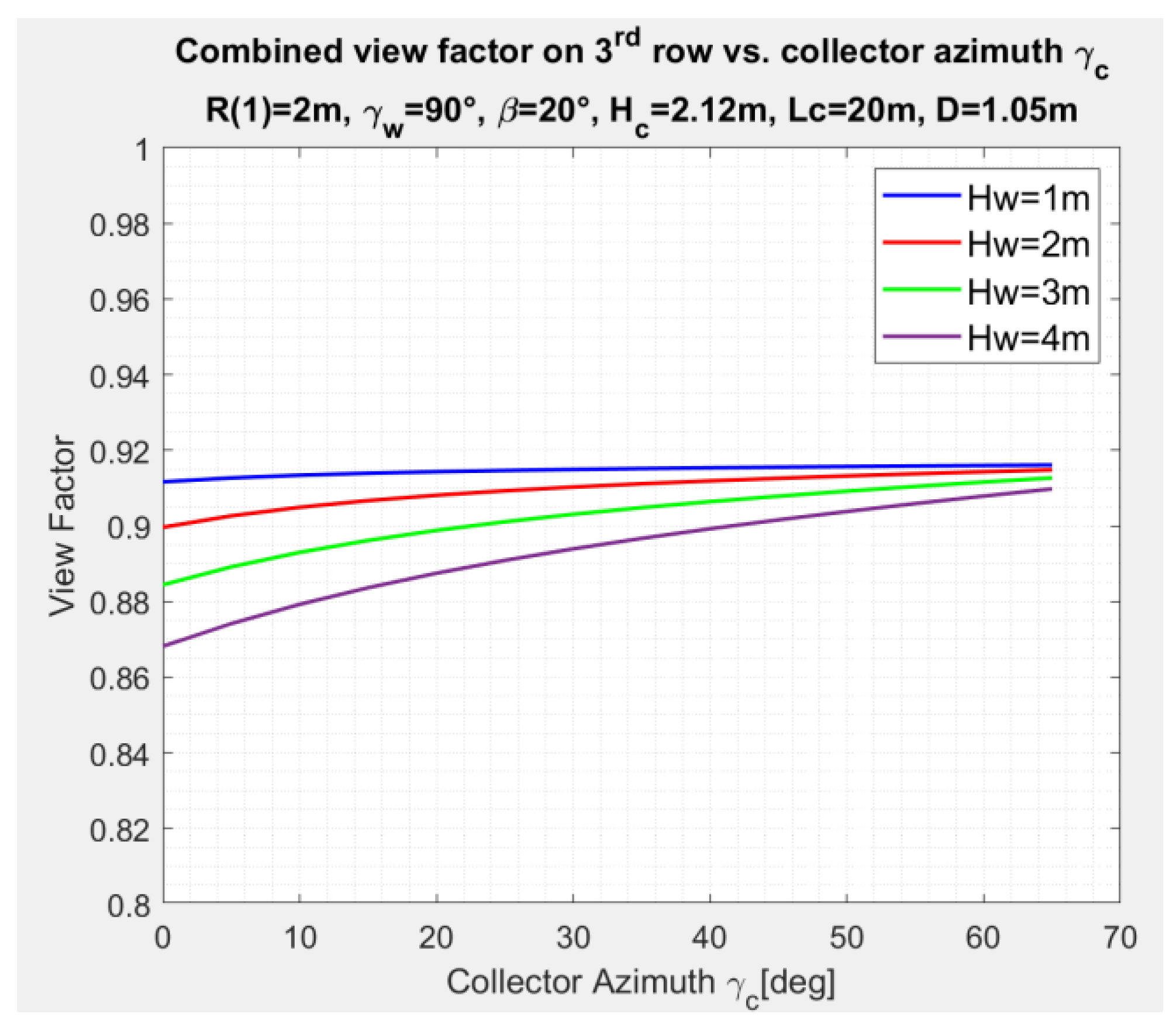
The effect of the variation of the collector azimuth angle ${\gamma }_C$ on the combined SVF, $V{F}^{conb.}$, for the deployment of collectors in Figure 6, is depicted in Figure 15 for collector number $K=3$, as an example. The calculations are based on Equations (5), (6), (8) and (10) and for $H_C=2.12 \mathrm{m},\beta =20°,D=1.05 \mathrm{m},L_C=20 \mathrm{m}$, wall height $H_W=1,2,3,4 \mathrm{m}$. Increasing the azimuth angle ${\gamma }_C$ increases the distance $R(K)$ (see Equation (8)); therefore, the SVF increases as shown in Figure 15. The effect of the collector azimuth angle on the SVF is small for larger azimuth angles.

3.3. Combined Sky View Factor, See Figure 7

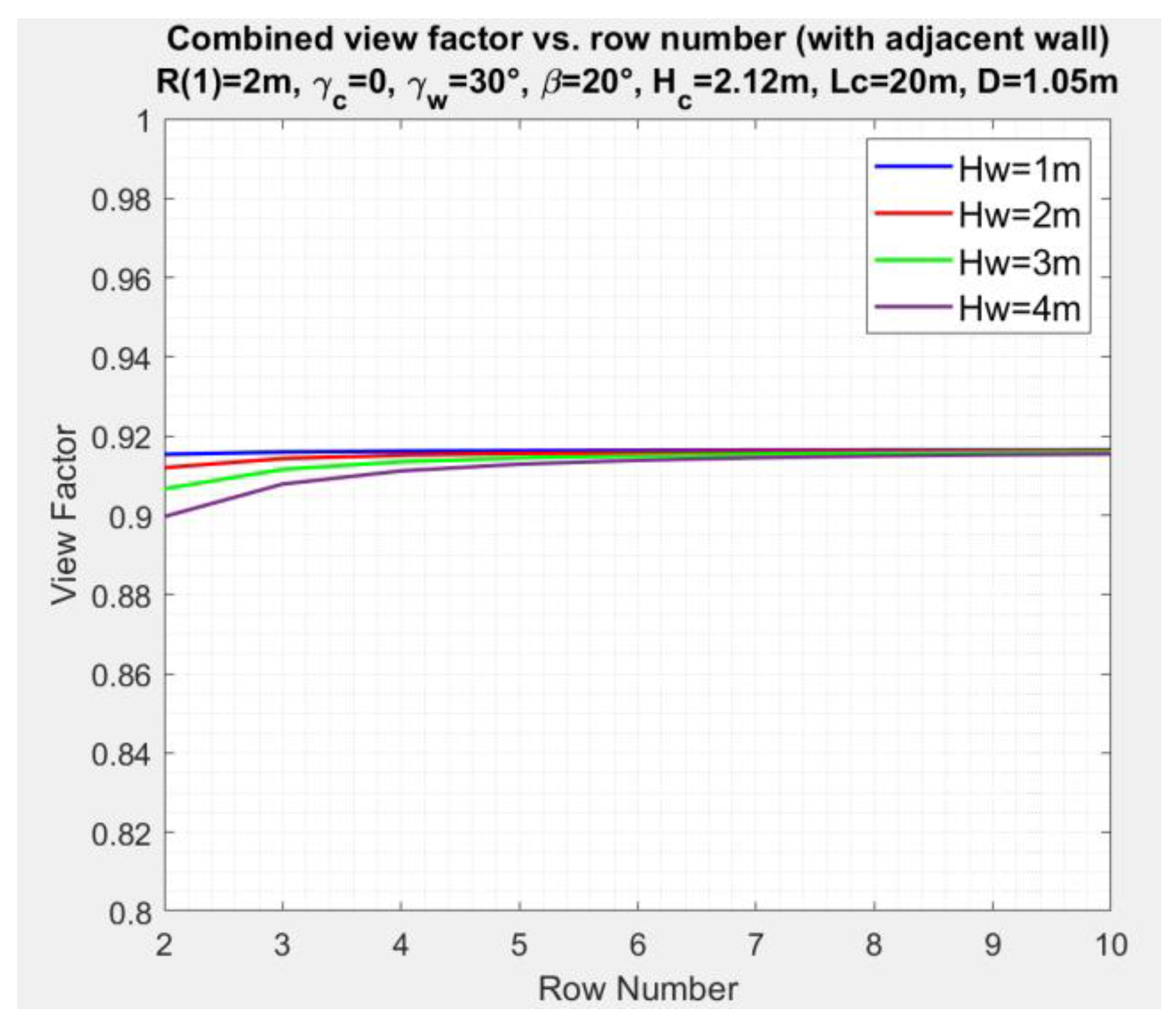
Figure 16 depicts the combined SVF, $V{F}^{conb.}$, of the second collector in a solar field as a function of the collector number $K$ for $R(1)=2 \mathrm{m}$. The calculation of the sky view factors corresponds to Equations (5), (6), (8) and (11) for $H_C=2.12 \mathrm{m},\beta =20°,D=1.05 \mathrm{m},L_C=20 \mathrm{m}$. The Figure shows a minor variation of the SVF with the collector row number $K$ for a wall azimuth angle ${\gamma }_W=30°$ and for different wall heights. The inter-row SVF value 0.9165, Equation (5), dominates the results.

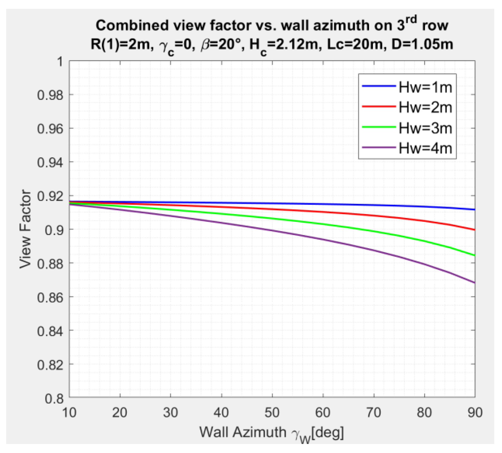
The effect of variation of the wall azimuth angle ${\gamma }_W$ on the combined SVF for deployment in Figure 7 is depicted in Figure 17, for collector number $K=3$, as an example. The calculation corresponds to Equations (5), (6) and (11), and for $H_C=2.12 \mathrm{m},\beta =20°,D=1.05 \mathrm{m},L_C=20 \mathrm{m}$, wall height $H_W=1,2,3,4 \mathrm{m}$. Decreasing the wall azimuth angle increases the distance between the wall and the collectors (see Equation (11)), therefore increasing the SVF.

3.4. Combined Sky View Factor, See Figure 8

The results for the sky view factors for the deployment in Figure 8 are the same as in Section 3.1.

Wall height may vary from 1.5 m for rooftop fences to 4 m and above, for building walls near PV collectors. The distance between walls and the collectors may vary depending on wall structures on the rooftops (small distances), and building walls across streets (large distances). The wall height, in the present study, varies between 1 and 4 m, and the distance between the wall and the collectors varies between 2 and 5 m. An example of the study shows that a wall of 4 m height at a distance of 2 m from the collectors and a collector length of 20 m, reduces the SVF by 6.2% (thus reducing the incident diffuse radiation on the collectors by 6.2%) as compared to the SVF of collectors installed in open space. The parameters that mostly affect the sky view factor are collector length $L_C$, wall height $H_W$, and distance $R$. The SVF of a horizontal plane $V{F}_R^h$ in the presence of a wall for collector length $L_C=10 \mathrm{m}$, the distance between the wall and the collector $R=2 \mathrm{m}$ and wall height $H_W=4 \mathrm{m}$ is 0.91, whereas for $L_C=20 \mathrm{m}$, it is 0.95. The $V{F}_R^h$ in the presence of a wall for $L_C=20 \mathrm{m}$, $H_W=4 \mathrm{m}$, and $R=2 \mathrm{m}$ is 0.91, whereas for $R=5 \mathrm{m}$, it is 0.97. The $V{F}_R^h$ in the presence of a wall for $L_C=20 \mathrm{m}$, $R=2 \mathrm{m}$, and $H_W=4 \mathrm{m}$ is 0.95, whereas for $H_W=2 \mathrm{m}$, it is 0.98. The inter-row sky view factor of the second and the subsequent rows $V{F}^C$ is 0.917; therefore, the combined SVF, $V{F}^{comb.}$, of a collector in the solar field, in the presence of a wall, is the product of the above view factors $V{F}_R^h$ and 0.917.

As the wall affects the incident diffuse radiation, Figure 18 shows the daily variation of the incident diffuse radiation, $\mathrm{W}/{\mathrm{m}}^2$, on a collector on May 1, for example, for a wall height of $4 \mathrm{m}$ (in blue) and for a wall height of $10 \mathrm{m}$ (in black) as compared to no wall in red. The wall is placed on the west side of the collectors, see Figure 5. The data for Figure 18 are $H_C=2.12 \mathrm{m},L_C=20 \mathrm{m},R=2 \mathrm{m},\beta =20°$. The figure clearly shows a reduction in the incident diffuse radiation with increasing wall height in the afternoon hours.

4. Discussion

PV systems, in urban environments, may also be deployed in areas between building walls on both sides of the systems. The calculation of the SVF, $V{F}_R^h$, of a horizontal plane, in the presence of walls, erected on both the east and west sides of the PV collectors may be based on the “cross-string rule” by Hottel [11]. This investigation is left for possible future work. The length of walls may be shorter than the available rooftop length for deployment of the PV systems. In this case, it would be necessary to modify the SVF, $V{F}_R^h$. The effect of higher walls and larger distances between walls and collectors on the sky view factors in the built environment may be investigated in an additional study. Published studies deal with sky view factors of PV systems deployed in open space, i.e., at locations without obscuring objects. Therefore, the motivation of the present study was to develop expressions and a methodology to determine the sky view factors of PV systems in the vicinity of walls.

5. Conclusions

Photovoltaic collectors deployed in multiple rows near the structure’s walls are partially obscured from the diffuse skylight, thus decreasing the incident diffuse radiation and resulting in diffuse radiation losses (masking losses). The diffuse radiation losses are associated with the SVF. The SVF of a collector stems from the inter-row SVF, $V{F}^C$, and from the SVF caused by the wall, $V{F}_R^h$. The combined SVF, $V{F}^{comb.}$, is the product of the two sky view factors: $V{F}^{conb.}=V{F}^C\times V{F}_R^h$, and by using the isotropic diffuse radiation model, the incident diffuse radiation on the collector thus becomes $V{F}^{comb.}{G}_{dh}$. This study investigates the parameters affecting the sky view factors. It includes the variation of the wall height, distance of the wall to the collectors, collector length, and collector and wall azimuth angles. The simulation results are drawn on the same scale to notice the range of variation for each studied case. The simulated results indicate that the overall range of the SVF variation may be quite noticeable and is between 0.78 (with a wall) and 0.97 (for no wall), for the parameters used in the study, meaning that the incident diffuse radiation may be reduced by about 20% in the presence of a wall. This reduction may be significant in locations with a high percentage of diffuse radiation.

The parameters that mostly affect the SVF are the collector length $L_C$, wall height $H_W$, and distance $R$. In summary, the simulation results indicate the following:

• The SVF increases for longer collectors and for lower wall heights.
• The SVF of a horizontal plane decreases for shorter distances from the collector to the wall.
• The effect of the collector azimuth angle on the SVF is small for larger azimuth angles.
• The SVF increases as the erected walls are more parallel to the collectors.

The study may assist the PV system designer in assessing the contribution of the incident diffuse radiation component to the generated electric energy for systems deployed near obscuring walls.