Prediction of Solar Flux Density Distribution Concentrated by a Heliostat Using a Ray Tracing-Assisted Generative Adversarial Neural Network

Abstract

Predicting the solar flux density distribution formed by heliostats in a concentrated solar tower power (CSP) plant is important for the optimization and stable operation of a CSP plant. However, the high temperature and blackbody attribute of the receiver makes direct measurement of the concentrated solar irradiance distribution a difficult task. To address this issue, indirect methods have been proposed. Nevertheless, these methods are either costly or not accurate enough. This study proposes a ray tracing-assisted deep learning method for the prediction of the concentrated solar flux density distribution formed by a heliostat. Namely, a generative adversarial neural network (GAN) model using Monte Carlo ray tracing results as the input was built for the prediction of solar flux density distribution concentrated by a heliostat. Experiments showed that the predicted solar flux density distributions were highly consistent with the concentrated solar spots on the Lambertian target formed by the same heliostat. This ray tracing-assisted deep learning method can be extended to other heliostats in the CSP plant and pave the way for the prediction of the solar flux density distribution concentrated by the whole heliostat field in a CSP plant.

1. Introduction

Concentrated solar power (CSP) is an important method of utilizing solar energy. When combined with thermal energy storage systems, CSP can offer stable and continuous power output during periods of high demand or unfavorable weather conditions. This can effectively address the intermittency issues associated with most other renewable energy sources [1]. It is well known that the concentrated solar flux density distribution at the receiver of the tower directly affects the working efficiency of the CSP station. However, it is difficult to directly measure the solar flux density distribution at the receiver. In the past two decades, several indirect methods have been proposed [2]. One indirect method is using heat flux meters installed on the receiver to obtain the heat flux values at some locations and then compute the solar density distribution on the basis of these discrete measurements and a thermal dynamic model of the receiver. Another indirect method is the photographic flux mapping method (PHLUX), which uses the same digital camera to capture images of the sun as well as the receiver [3]. The solar density distribution on the receiver was then calculated on the basis of the images and calibrated reflectivity of the receiver. This method consists of several tedious steps and is costly. In addition, it is not applicable to CSP stations with cavity-type receivers or other blackbody-type receivers [4]. As the proposed measuring methods are either costly or not applicable in real scenarios, simulations have been used for the prediction of solar flux density in CSP.

Currently, the simulation models adopted for the prediction of solar flux density distribution formed by heliostats can be classified into two categories. One category uses the Monte Carlo ray tracing (MCRT) method and another category employes analytical method [5]. Analytical methods normally assume that the flux density distribution of heliostats take the form of Gaussian functions and that the distribution can be estimated via data fitting or interpolation [6]. This avoids the complex ray tracing process and has been implemented in various simulation tools such as DELSOL, HFLCAL, SolarPILOT, and FluxSPT [7]. However, the accuracy achieved with these analytical models is far from satisfactory. Compared with analytical models, the MCRT methods normally give better results [8]. Existing simulation models using MCRT method include SolTrace, MIRVAL, Tracer, STRAL, Solfast4D, and the web application OTSunWebApp v0.7.6 [7,8,9,10]. Given enough computation time, the MCRT-based simulation models can output a prediction of the solar flux density distribution of a large-scale heliostat field at high resolution. But the results achieved are still not satisfactory, as the geometric errors and reflectivity differences of the reflecting surface of heliostats cannot be measured and taken into account in simulations.

With the rapid advancement of artificial intelligence, deep learning methods have been applied in many science and engineering fields. In the CSP field, deep learning techniques have been used to generate the aiming strategies of heliostats under varying solar angles and on cloudy days [11]. A model-free deep reinforcement learning and soft actor–critic algorithm was used to optimize the aiming strategies of heliostats to improve the concentrating efficiency of a CSP [12]. Some researchers proposed a method for predicting the irradiance flux density distribution using lunar light, and a computational model of lunar irradiance flux density has been established for dish concentrators under different lunar conditions [13]. However, the accuracy achieved with the lunar prediction method is not satisfactory. Several factors, e.g., the differences in the angular size and profiles of the solar disk vs. the lunar disk, and the interference of background lighting in the night sky, affect the prediction accuracy of the lunar method [14].

Researchers are also investigating the application of deep learning to the prediction of solar flux density distribution. Conditional generative adversarial networks have been proposed for predicting the solar density distribution of a heliostat based on lunar spots focused by a heliostat on a Lambertian target [15]. A data-driven method based on the StyleGAN architecture was proposed for the prediction of solar flux density by German researchers from the DLR [16]. A differentiable ray tracing method based on the captured calibration image of heliostat has been proposed for metric evaluations in CSP [17]. According to the paper, the differential ray tracing method achieved a prediction accuracy comparable with that of deflection measuring method [17]. A framework for a modern SCADA system in a CSP plant, integrating OPC UA, WiFi mesh networks, and deep learning algorithms, has been proposed for the improvement of the performance and the reduction of running costs [18].

Because the concentrated solar flux density of a heliostat is affected by many factors, for example, the incident angle of sunlight, the surface geometry of the heliostat, the surface quality of the heliostat, the reflectivity of the surface, the air temperature, and the humidity in the air, it is difficult to build an analytical model for the prediction of solar flux distribution. Deep learning models provide a good means of representing the complex effects of numerous factors on the solar flux density distribution of a heliostat. A Monte Carlo ray tracing-assisted generative adversarial network model is thus proposed for the prediction of solar flux density distribution in this study. The model is built on the Pix2Pix framework and trained using simulated spots from Monte Carlo ray tracing together with captured light spots on the Lambertian target as the inputs. Experimental results show that the model can generate accurate predictions of the solar flux density distribution concentrated by the heliostat. The proposed method can be extended to any other heliostat in the heliostat field. The solar flux density distribution of the whole heliostat field can thus be predicted on the basis of the combination of different GAN models for various heliostats.

2. Materials and Methods

A CSP station typically comprises tens of thousands of heliostats. Each heliostat tracks the movement of the Sun and reflects the sun’s rays onto the receiver positioned on top of the central tower. With prior knowledge of the physical parameters of the heliostat field, Monte Carlo-based ray tracing is a reliable way to obtain structural information on the concentrated solar energy density of the receiver. In the following text, the details of the ray-based simulation of a heliostat field and the design of the generative GAN model for the prediction of the solar flux distribution are presented.

2.1. Solar Radiation

Building a proper mathematical model for the radiation of the sun is the first step towards analyzing the solar irradiance density distribution. The pillbox model [19], the Gaussian distribution model [20], and Buie’s model [21] have been previously adopted in many solar radiation-related simulations. According to Buie’s model, terrestrial solar radiation simulation should consider the combined effects of both the central solar disk (with a half angle of 4.65 milli-radians, or 0.265°) and the circumsolar region (the half angle is between 0.265° and 2.5°). The radiation density is greatest within the disk and diminishes toward the circumsolar region, resulting in the characteristic halo effect of the sun [21]. As this research focuses on the use of deep learning models for the prediction of solar flux distribution, Buie’s sun shape model is not adopted for the ray tracing simulation. Instead, a simpler sun shape model [22], as shown in Equation (1), which consumes less computation time, is employed in the ray tracing process.

$$S\left(\alpha \right)=\left\{\begin{array}{cc}\hfill S_0(1-\lambda {\left({\displaystyle \frac{\alpha }{{\alpha }_{\mathrm{s}}}}\right)}^4),& \alpha \le {\alpha }_{\mathrm{s}}\hfill \\ \hfill 0,& \alpha >{\alpha }_{\mathrm{s}}\hfill \end{array}\right.$$

(1)

In Equation (1), S(α) represents the radiation flux at an emitting angle α, λ is a constant equaling 0.5138, and S₀ indicates the maximum energy flux at the center. The solar cone angle α_s is 4.65 milli-radians, as depicted in Figure 1. The solar radial flux density distributions of three models are compared in Figure 1b, where the blue curve represents the adopted sun shape model, the green dashed line represents the pillbox model, and the orange dashed line represents the Gaussian model.

2.2. Sun Tracking Process of a Heliostat

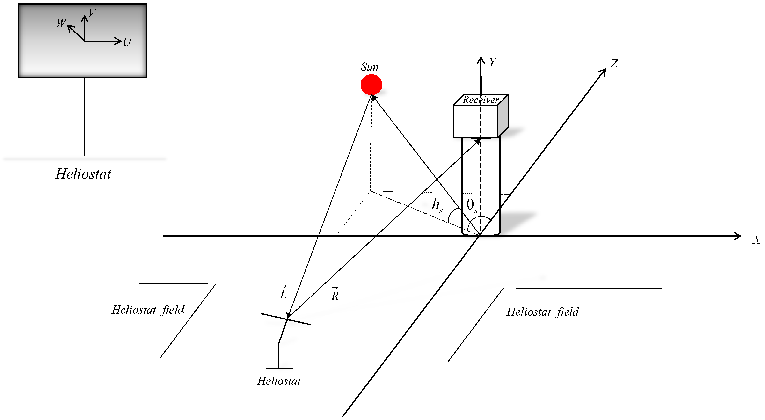
The coordinates of each heliostat and the aimed target were used to determine the normal direction of the reflecting surface of the heliostat at a specific time. The modeling of the sun tracking process involves three coordinate systems, namely the global coordinate system, the heliostat coordinate system, and the receiver coordinate system, as shown in Figure 2. The global coordinate system takes the east as the X axis, north as the Z axis, and the zenith as the Y axis. The origin of the global coordinate system is located at the bottom of the tower.

For the heliostat coordinate system, the origin is at the center of the heliostat’s surface, with the U axis parallel to the longer edge of the heliostat’s surface, the V axis parallel to the shorter edge of the heliostat’s surface, and the W axis perpendicular to the surface. The receiver coordinate system is defined as a two-axis system on the target plane, with the origin at the center of the receiver and two axes along the horizontal and vertical directions, respectively.

The position of the sun can be described using the solar elevation angle and solar azimuth angle in the world coordinate system. The solar elevation angle ${\alpha }_{\mathrm{s}}$ is defined as the angle between the solar vector $\overrightarrow{L}$ and the horizontal plane. The solar azimuth angle ${\beta }_{\mathrm{s}}$ is the angle between the projection of the solar vector $\overrightarrow{L}$ onto the horizontal plane and the positive north direction, i.e., the Z axis. The solar elevation and azimuth angles can be calculated using the following formulas

$$\left\{\begin{array}{c}sin\left({\alpha }_{\mathrm{s}}\right)=sin\left(\varphi \right)sin\left(\delta \right)+cos\left(\varphi \right)cos\left(\delta \right)cos\left(\omega \right)\\ sin\left({\beta }_{\mathrm{s}}\right)={\displaystyle \frac{cos\left(\delta \right)sin\left(\omega \right)}{cos\left(h_{\mathrm{s}}\right)}}\\ cos\left({\beta }_{\mathrm{s}}\right)={\displaystyle \frac{sin\left(\varphi \right)sin\left(h_{\mathrm{s}}\right)-sin\left(\delta \right)}{cos\left(\varphi \right)cos\left(h_{\mathrm{s}}\right)}}\end{array}\right.$$

(2)

where $\varphi$ is the latitude of observer, δ is the declination angle of the sun, and ω is the hour angle, which can be computed using the Cooper equation [23]. The vector of solar rays $\overrightarrow{L}$ can thus be expressed as follows:

$$\overrightarrow{L}=\left[\begin{array}{c}cos{\alpha }_{\mathrm{s}}·sin{\beta }_{\mathrm{s}}\\ cos{\alpha }_{\mathrm{s}}·cos{\beta }_{\mathrm{s}}\\ sin{\alpha }_{\mathrm{s}}\end{array}\right]$$

(3)

Considering the distribution of the solar energy flux density, the sun’s cone angle and its position at a specific time cannot be ignored. The other incident rays are represented as a vector offset from the main incident ray $\overrightarrow{L}$, as illustrated in Figure 3. For any nonparallel ray $\overrightarrow{H}$ within the light cone, its vector is given by:

$$\overrightarrow{H}={\displaystyle \frac{(\overrightarrow{L}+\overrightarrow{t})}{|\overrightarrow{L}+\overrightarrow{t}|}}$$

(4)

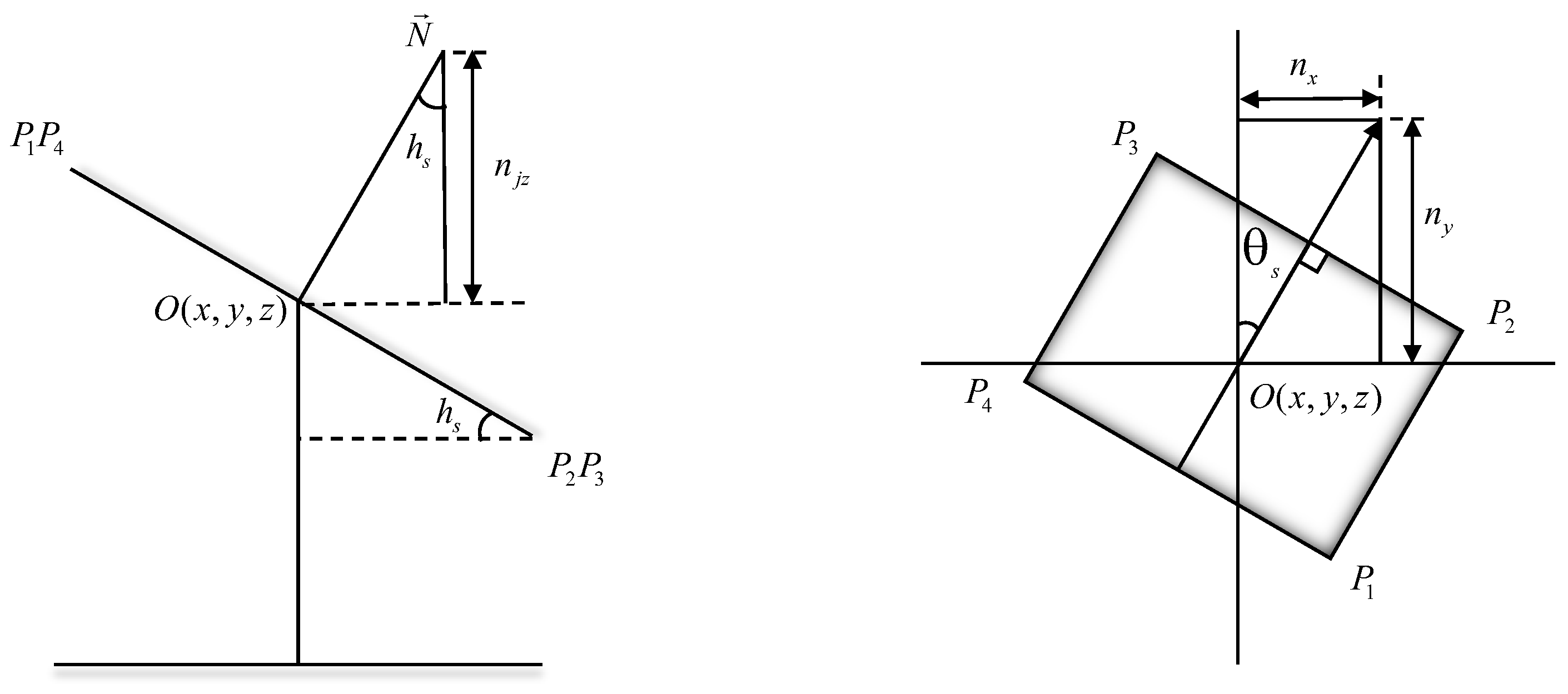
Assume that $\overrightarrow{N}$ is the normal vector of the heliostat’s surface. The angle between $\overrightarrow{N}$ and the zenith is the heliostat’s elevation angle $h_{\mathrm{s}}$. Figure 4 (left) is a side view of the heliostat. The elevation angle can thus be expressed as in Equation (5), where $n_{jz}$ is the Z coordinate of $\overrightarrow{N}$ in the heliostat coordinate system. Figure 4 shows the side and top views of the heliostat.

$$cos{h}_{\mathrm{s}}=n_{jz}sin{h}_{\mathrm{s}}=\sqrt{1-n_{jz}^2}$$

(5)

The azimuth angle of the heliostat can be expressed using the coordinates of the normal vector $\overrightarrow{N}$, as follows:

$${sin\theta }_s=-n_{jx}/\sqrt{n_{jx}^2+n_{jy}^2}{cos\theta }_s=-n_{jy}/\sqrt{n_{jx}^2+n_{jy}^2}$$

(6)

In the heliostat coordinate system, the rotation of the heliostat is represented by the angles $h_{\mathrm{s}}$ and ${\theta }_{\mathrm{s}}$. Assuming that the heliostat is located in the first quadrant of the coordinate system, the rotation of the heliostat can be regarded as rotating at $-h_s$ around the horizontal direction, and then rotating at $-{\theta }_s$ around the vertical direction. The global coordinates $P^W$ of a point can thus be obtained by multiplying the rotation matrix with the local coordinates $P_i^w$ in the heliostat coordinate system, as shown in Equation (7).

$$P^W=\left[\begin{array}{ccc}cos\left({\theta }_{\mathrm{s}}\right)& cos\left(h_{\mathrm{s}}\right)& sin\left({\theta }_{\mathrm{s}}\right)\\ -sin\left({\theta }_{\mathrm{s}}\right)& cos\left({\theta }_{\mathrm{s}}\right)& cos\left(h_{\mathrm{s}}\right)\\ 0& -sin\left(h_{\mathrm{s}}\right)& cos\left(h_{\mathrm{s}}\right)\end{array}\right]·P_i^w$$

(7)

2.3. Monte Carlo Ray Tracing for the Concentrated Solar Flux

Monte Carlo ray tracing (MCRT) is used to obtain the coarse information of the concentrated solar flux density distribution. MCRT uses discretely sampled rays to simulate the light source and tracks the paths of the light rays in accordance with the physical laws in the real world. With ongoing advancements in computing and digital display hardware, high-resolution ray tracing has become affordable for the simulation of optical fields.

In the ray tracing process, spatial validations are frequently used to check whether a ray intersects the surface of a heliostat. The reflecting surface of each heliostat is restricted by the four corner points in the heliostat coordinate system. The orientation of the heliostat can be theoretically calculated on the basis of the coordinates of the heliostat center (x,y,z). The normal vector $\overrightarrow{N}$ of the heliostat’s surface can be computed using the incident light vector $\overrightarrow{H}$ and the reflected light vector $\overrightarrow{R}$, which is decided by the coordinates of the heliostat center and the aimed point, i.e., the center of receiver (0,0,A) in this case, as shown in Equation (8).

$$\begin{array}{c}\overrightarrow{R}={\displaystyle \frac{\left(-x,-y,A-Z\right)}{\left|\overrightarrow{R}\right|}}\\ \overrightarrow{N}={\displaystyle \frac{(\overrightarrow{H}+\overrightarrow{R})}{\left|\overrightarrow{H}+\overrightarrow{R}\right|}}\end{array}$$

(8)

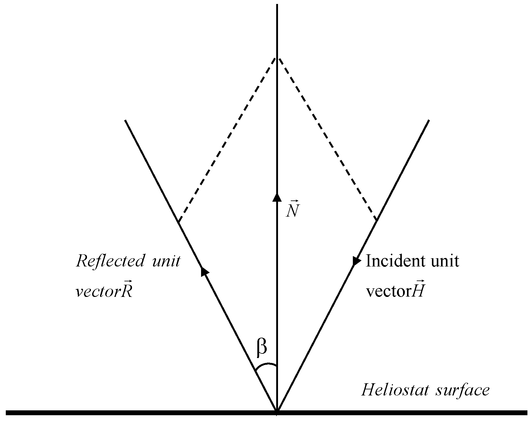
During the ray tracing process, directional rays are generated and sampled according to the distribution of the light source. The rays pass through the atmosphere and arrive at the heliostat and are then reflected by the surface onto the receiver atop the tower. Because the normal vector of the heliostat is known, for each generated ray, the corresponding reflecting ray can be obtained on the basis of the principle of symmetry for mirror reflection, as shown in Figure 5.

The concentrated solar flux density on the receiver is influenced by several factors, including the density of solar radiation, the geometric shape of the surface, and the bidirectional reflecting distribution functions of the heliostats. Assuming that the surface of the heliostat is a planar surface denoted by Ω, and ignoring the aiming accuracy of the heliostat, the sun rays reflected by the heliostat can be expressed using the following formula

$$R\left(x,y,z,{\omega }_0\right){|}_{(x,y,z)\in \mathsf{\Omega }}=\int f\left(x,y,z,{\omega }_i,{\omega }_0\right)L\left(x,y,z,{\omega }_i\right)({\omega }_i·n)d{\omega }_i$$

(9)

where R(x,y,z,ω₀) describes the light rays reflected at a point (x,y,z) on the heliostat at a solid angle of ω₀, ω_i is the solid angle of the incident light, the range of ω_i is related to the subtended angle of the sun, f(x,y,z,ω_i,ω₀) denotes the bidirectional reflecting function of the heliostat at point (x,y,z), L(x,y,z,ω_i) denotes the intensity of the incident light at the point, and $n$ is the surface normal at the point. Suppose that the heliostat’s surface is planar and the normal reflectivity is same across the planar surface, which means that f(x,y,z,ω_i,ω₀) in Equation (9) can be seen as a scalar, denoted as ρ in Equation (10), during the ray tracing process. The dot product ${\omega }_i·n$ can be represented by $cos{\theta }_i$, which represents the cosine angle of the incident ray with respect to the normal of the surface.

The light ray reflected by the heliostat falls on the receiver or on a Lambertian target during the calibration process, forming a light spot that can be captured using a digital camera. The intersection points can be calculated for each ray as the geometrical plane of the receiver or the target is known. The solar flux at a point [x,y,z], which corresponds to the intersection of the light rays R(x,y,z,ω₀) with the receiver, can thus be expressed as Equation (10)

$$E\left(x,y,z\right)=\iint R(x,y,z,{\omega }_0){\eta }_{Atm}d{\theta }_{0}d{\phi }_0\approx {\eta }_{Atm}{\sum }_{{\phi }_0}{\sum }_{{\theta }_0}\rho L\left({\omega }_i\right)cos{\theta }_i$$

(10)

where ${\eta }_{Atm}$ is the transmission attenuation factor in the mirror field, which can be calculated on the basis of the distance between the heliostat and receiver according to the empirical model proposed by [22].

$$\begin{array}{c}{\eta }_{Atm}=f\left(x\right)=\left\{\begin{array}{cc}\hfill 0.99321-1.176\times {10}^{-4}·D+1.97\times {10}^{-8}·D^2,& D<1000\mathrm{m}\hfill \\ \hfill e^{-0.0001106D},& D\ge 1000\mathrm{m}\hfill \end{array}\right.\end{array}$$

(11)

The final stage of the simulation is to collect the results from multiple threads of the ray tracing processes. The receiver is divided into two dimensional grids of cells along the horizontal and vertical directions. Each traced ray is mapped to the corresponding bin of the grid cells on the basis of the location of the beam intersection and the boundaries of each bin. The number of intersections for each bin are added up during the ray tracing process and stored in a matrix.

The matrix obtained is then converted into a grayscale image using a function named imagesc in MATLAB R2024a. The element values in the matrix are first normalized using (12)

$$\begin{array}{c}{c}_{ij}^{\prime }={\displaystyle \frac{c_{ij}-\min \left(C\right)}{\max \left(C\right)-\min \left(C\right)}}\end{array}$$

(12)

where $c_{ij}^{\prime }$ represents the normalized value, which is then used for mapping from a float value between [d_min,d_max] to a color map range in [1, N]. The mapping formula is given by Equation (13):

$$\begin{array}{c}index=\left[{\displaystyle \frac{\left(c_{ij}^{\prime }-d_{min}\right)}{\left(d_{max}-d_{min}\right)}}\times (N-1)\right]\end{array}+1$$

(13)

To check whether Gaussian noise helps the learning process, the color map produced with MCRT is processed further using a Gaussian smoothing filter. The Gaussian filter has a size of 13 × 13, with its peak value equal to 0.159. The smoothing process involves a convolution between the color map and the selected Gaussian kernel, as shown in Equation (14).

$$I_{mooths}(x,y)=I(x,y)\ast G(x,y)=\sum \sum I(m,n)·G(x-m,y-n)$$

(14)

2.4. Prediction of Solar Flux Density Distribution Using an MCRT-Assisted GAN Model

The concentrated solar density distribution of a heliostat depends on the density of the incident light, the incident angles, the surface geometry of the heliostat, and the reflectivity of the surface. The incident angle and density of solar radiation can be calculated using physical laws or mathematical models. However, the reflectivity and the surface geometry of the heliostat are not constant. The actual values of these variables are hard to measure online. To learn the reflecting properties of the heliostat surface, an approach combining MCRT and a generative adversarial network (GAN) is thus proposed.

Generative adversarial networks have achieved great success in image generation and many other fields [24,25]. A typical GAN consists of a generator network that produces samples and a discriminator network that discriminates the generated fake sample from the real sample. In this approach, the simulation result at a certain time produced by MCRT is used as the condition. The previously captured light spots on the Lambertian target concentrated by the heliostat are used as real samples of solar flux distribution. A conditional GAN model can then be trained for the prediction of the concentrated solar density distribution formed by the heliostat, as shown in Figure 6. The concentrated light spots on the Lambertian target were captured using a calibrated camera. These images contain full information on the surface geometry as well as the reflectivity attributes of the specific heliostat, and therefore provide efficient data for learning and modeling.

The framework of Pix2Pix, a well-known cGAN model, was used in this research. The generator network of Pix2Pix is a UNet, as shown in Figure 7. By directly linking the encoder and decoder pairs in the network, the skip connections in the UNet can preserve the features of different levels.

PatchGAN is used in the discriminator of Pix2Pix. PatchGAN evaluates images’ authenticity using localized patches rather than entire images. For example, to evaluate the generated flux density image, PatchGAN produces an authenticity matrix, where each element X_ij represents a patch’s score, as shown in Figure 8. The parameter PatchSize, namely, N in Figure 8, significantly influences the generated images’ quality and the training process.

The objective function for the training process is defined on the basis of the combination of discriminator loss and the L1 loss of the generator. The discriminator loss function ${\mathcal{L}}_{GAN}(G,D)$ is as shown in Equation (15). The generator loss function is shown in Equation (16). Equation (17) is the mathematical expression of total loss used for training.

$${\mathcal{L}}_{GAN}(G,D)={\mathbb{E}}_{x,y}\left[\mathit{log}D\right(x,y\left)\right]+{\mathbb{E}}_x[\mathit{log}(1-D(x,G\left(x\right)\left)\right)]$$

(15)

$${\mathcal{L}}_{L1}\left(G\right)={\mathbb{E}}_{x,y}[\Vert y-G(x\left){\Vert }_1\right]$$

(16)

$${\mathcal{L}}_{total}(G,D)={\mathcal{L}}_{GAN}(G,D)+\lambda {\mathcal{L}}_{L1}\left(G\right)$$

(17)

In Equations (15)–(17), $l\mathit{og}D(x,y)$ represents the logarithm of the discriminator outputs for the real image pairs (x,y), D(x, G(x)) represents the discriminator outputs for the generated images (x, G(x)), ${\mathbb{E}}_{x,y}\left[\mathit{log}D\right(x,y\left)\right]$ denotes the cross-entropy of the discriminator outputs for the variables x and y, ${\mathbb{E}}_x[\mathit{log}(1-D(x,G\left(x\right)\left)\right)]$ denotes the cross-entropy of the discriminator outputs for x and the generated image G(x), ${\mathbb{E}}_{x,y}[\Vert y-G(x\left){\Vert }_1\right]$ denotes the cross-entropy of the L1 distance between the generated image G(x) and the real image y.

3. Experiments and Analysis of Results

To evaluate the proposed method, experiments were organized, and a dataset was built using the reflected light spots of a heliostat located at Dahan CSP station, Beijing. The geographical position and geometric parameters of the heliostat and target are listed in

Table 1. Parameter settings for the ray tracing simulation.

Heliostat Field Parameters	Simulation Values	Heliostat Field Parameters	Simulation Values
Longitude/E	115.94°	Heliostat size	10 m × 10 m
Latitude/N	40.38°	Heliostat coordinates	(0; 26.7; 5.78)
Average altitude/m	40	Receiver coordinates	(0; 74; 74.5)
Number of points	40 million	Receiver size	5 m × 5 m

. Both MCRT simulation and AI learning were carried out on a computer equipped with an Intel Core i711700 CPU (Intel, Santa Clara, CA, USA) (2.50 GHz) and an NVIDIA GeForce RTX 3080 Ti card (NVIDIA, Santa Clara, CA, USA).

Images of the concentrated solar spots produced by Heliostat #7, collected for the study of the lunar concentration distribution [13], were employed to construct the dataset. Simulations were carried out for Heliostat #7 with known parameters and a selected time. The images of the solar spots concentrated by Heliostat #7 and captured on 1 March and 2 March 2023 were selected as the target data for the training of the Pix2Pix model. Selected data were mainly from the periods of 12:45–13:45 p.m. and 14:55~15:55 p.m. on 1 March 2023, and the periods of 9 a.m.~10 a.m. and 11 a.m.~12 a.m. on 2 March 2023. In total, 970 pairs of data were used to train the MCRT_Pix2Pix model.

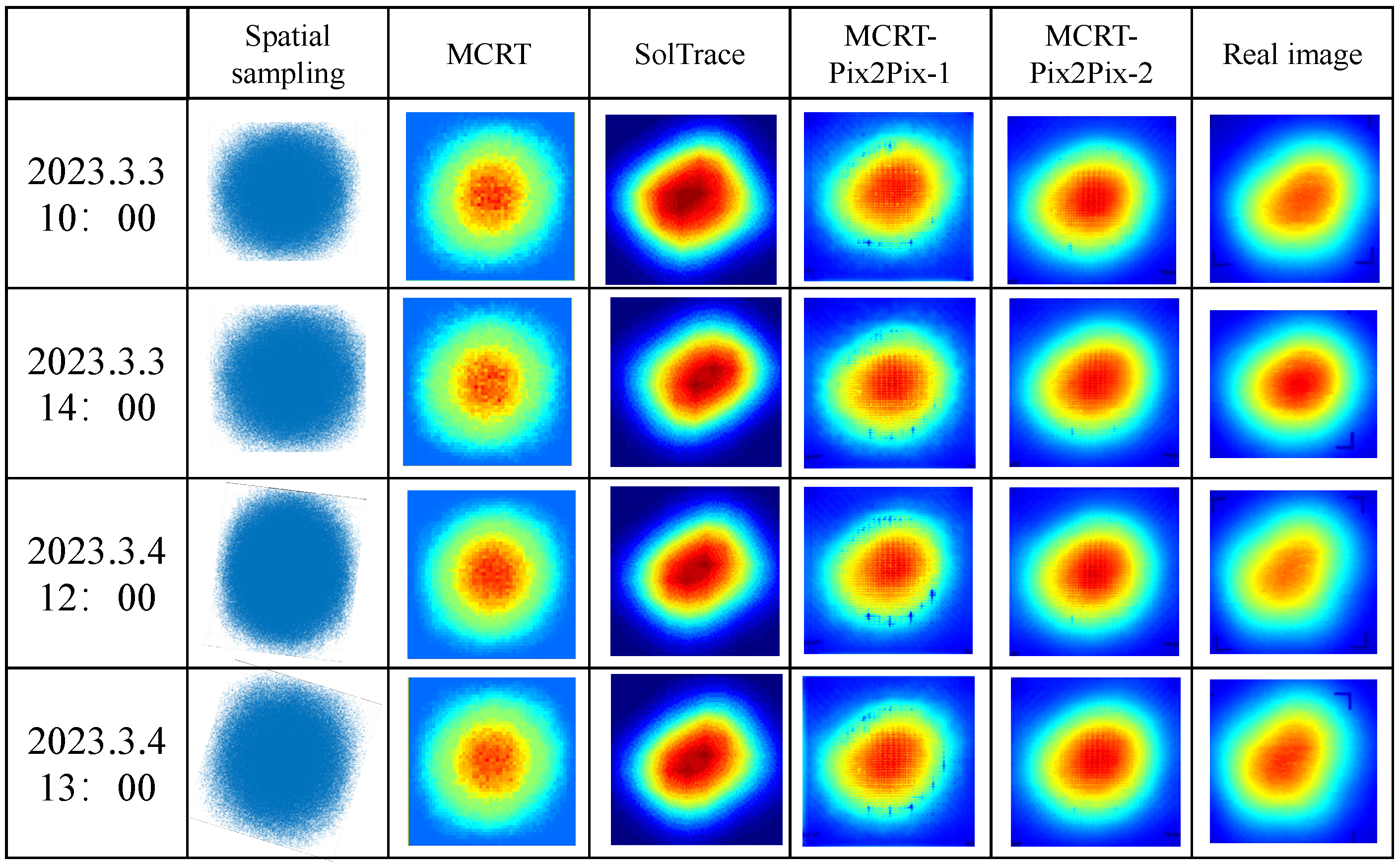
Two MCRT-assisted GAN models were trained: MCRT-Pix2Pix-1 using original MCRT images, and MCRT-Pix2Pix-2 using smoothing-filtered MCRT images. Both models showed similar performance during testing, as shown in Figure 9, which compares images generated from point clouds, MCRT, SolTrace, and both GAN models at four times (different from the training data’s date), along with captured images of concentrated solar spots on the Lambertian target.

It can be observed that the images generated by both MCRT-Pix2Pix models highly resemble the real images. As comparisons, the original MCRT result and the result from SolTrace (a well-known simulation tool in CSP) are shown together in Figure 9. The MCRT result is the input to the GAN model and is produced using the sun shape model introduced in Section 2.1. The result of SolTrace is obtained by using the pillbox sun shape model and setting the slope error as well as the specular errors to zero. The poor accuracy of SolTrace may be partially due to the ideal assumptions of these variables. However, the improvements in the generated images over the results of MCRT are also significant. To evaluate the performance of the ray tracing-assisted GAN model, different metrics have been selected to compare the generated samples and the real images.

3.1. Evaluation Metrics

The structural similarity index measure (SSIM) is a metric used to quantify the similarity between two images [26]. The SSIM has three key properties: symmetry, boundedness, and uniqueness. These features make the SSIM very effective for medical imaging, remote sensing, and compression quality assessment [14,27]. The SSIM measures images’ similarity by evaluating and combining weighted differences in brightness, contrast, and structure, thereby providing a comprehensive quality assessment, as shown in Equation (18).

$$\mathrm{SSIM}\left(x,y\right)={\displaystyle \frac{\left(2{\mu }_x{\mu }_y+C1\right)\left(2{\sigma }_{\mathrm{xy}}+C2\right)}{\left({{\mu }_x}^2+{{\mu }_y}^2+C1\right)\left({{\sigma }_x}^2+{{\sigma }_y}^2+C2\right)}}$$

(18)

Cosine similarity is widely used to compare two vectors or two matrices during signal processing. Discrete Fourier transform (DFT) can be used to find the spectrum of a digital image. The Fourier spectrum of an image reveals spatial variations in the irradiance on the subject at different spatial spans. After obtaining the spectrum of each image, the cosine similarity of the spectrum was calculated using Equation (19), where A_i and B_i represent the ith component of the spectrum vector.

$$cos\left(\theta \right)={\displaystyle \frac{A·B}{‖A‖‖B‖}}={\displaystyle \frac{\sum _{i=1}^n{A}_i{B}_i}{\sqrt{\sum _{i=1}^n{A}_i^2}\sqrt{\sum _{i=1}^n{B}_i^2}}}$$

(19)

The peak signal to noise ratio (PSNR), measured in decibels (dB), is another metric widely used for the evaluation of image quality, particularly in compression and reconstruction applications. To compute the PSNR, the mean square error (MSE) between the original image I and the reconstructed image K must be computed first. The formula for calculating the MSE is given in Equation (20). Equation (21) was used to calculate the PSNR.

$$\mathrm{MSE}={\displaystyle \frac{1}{mn}}{\sum }_{i=0}^{m-1}{\sum }_{j=0}^{n-1}\left[I\right(i,j)-K(i,j){]}^2$$

(20)

$$\mathrm{PSNR}=10·log\left({\displaystyle \frac{\mathrm{MA}{\mathrm{X}}^2}{\mathrm{MSE}}}\right)$$

(21)

where MAX denotes the maximum of the pixel values in the image.

3.2. Comparisons and Analysis

Forty images of light spots concentrated by the heliostat and captured on the dates of 3 March and 4 March 2023 using a digital camera were selected to evaluate the prediction accuracy of the MCRT-assisted GAN models. As the performance of MCRT_Pix2Pix_2, the model trained using Gaussian smoothed images of simulation results, was similar to that of MCRT_Pix2Pix_1, only comparison results between the images generated with MCRT_Pix2Pix_1 (denoted MCRT_Pix2Pix in the following text) and the real images are shown below.

3.2.1. Structural Similarity Index Measure

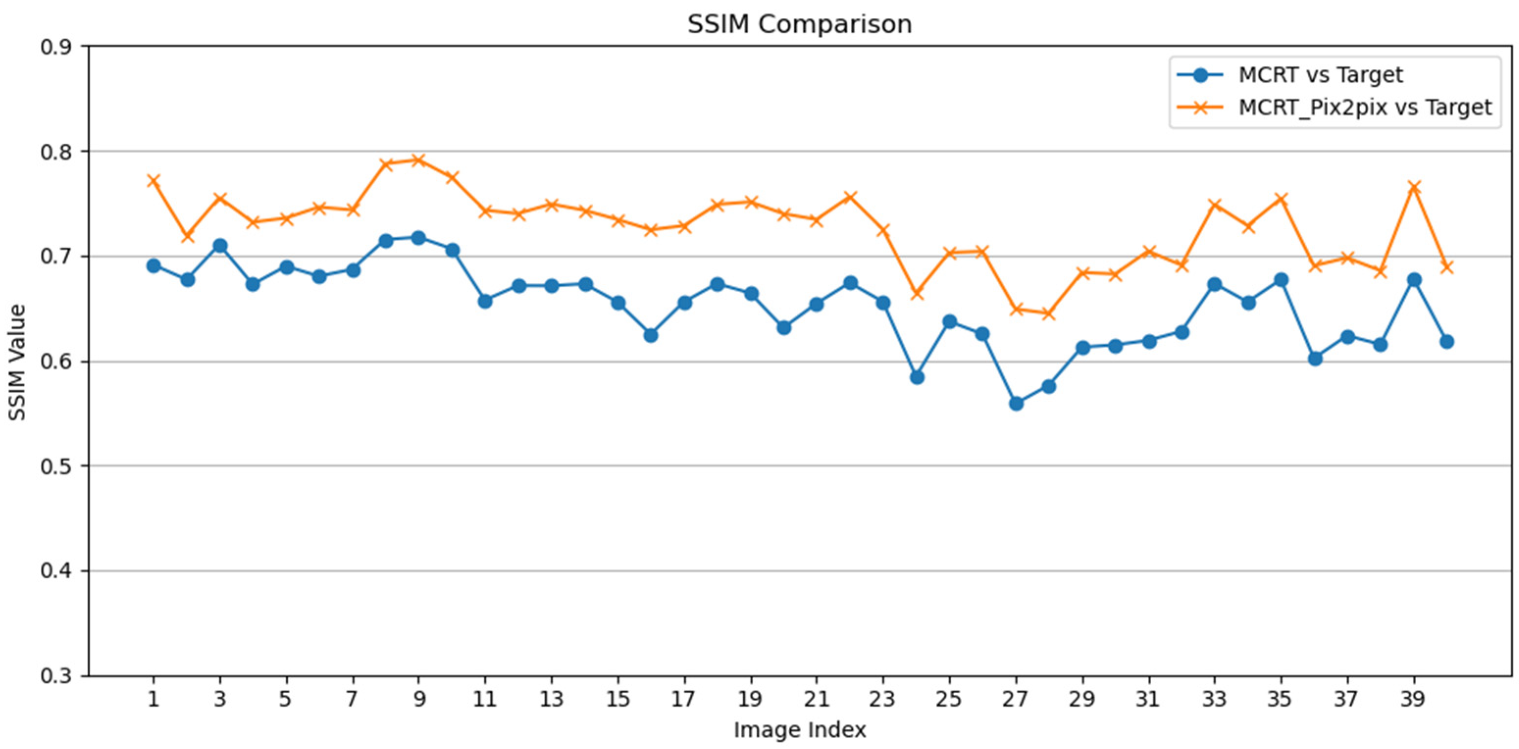
The SSIM between the generated images of the MCRT_Pix2pix model and the actual concentrated solar spots of the heliostat were calculated and compared. The results showed that the generated images of MCRT_Pix2Pix had a significant improvement in terms of the SSIM, as illustrated in Figure 10. The mean SSIM value between the simulations and the real images in the test dataset was approximately 0.65, whereas the mean SSIM between the images generated with MCRT_Pix2Pix and the real images increased to 0.73. This indicates that the MCRT_Pix2Pix models provide better predictions of concentrated solar density distribution than pure MCRT simulations.

For the whole test dataset, the variance of the SSIM with the MCRT group was 0.0014, and the variance of the SSIM with the MCRT_Pix2Pix model was 0.0012. The smaller variance implies that the stability of the MCRT_Pix2Pix model is as good as that of the simulation, which is of great significance for the consistent performance of the model in predicting the solar density distribution.

3.2.2. Cosine Similarity of Images

The average cosine similarity between the simulation result and the real images was 0.91, whereas the average cosine similarity between the images generated with MCRT-Pix2Pix and the actual images was approximately 0.94. Both groups were high, but the MCRT-Pix2Pix images were consistently better than those of the MCRT group for all test samples, as illustrated in Figure 11.

3.2.3. Cosine Similarity of the Spectrum

In the spatial frequency domain, MCRT_Pix2Pix achieves a higher average value in terms of cosine similarity than MCRT. In addition, the MCRT_Pix2Pix group has much less fluctuation in terms of spectral cosine similarity, as illustrated in Figure 12a. Comparisons of the cosine similarity of the central 64 × 64 pixels’ part of the spectrum (the low-frequency part of the spectrum), as shown in Figure 12b, also demonstrate that the images generated with MCRT-Pix2Pix are highly consistent with the real images, with the spectral cosine similarity reaching 0.9958.

3.2.4. PSNR

The PSNRs between the generated images and real images were also calculated for both MCRT and MCRT_Pix2Pix. The results are shown in Figure 13. The PSNRs for both groups were not high due to the low contrast of concentrated spots. Nevertheless, the average PSNR of the generated images from MCRT_Pix2Pix was approximately 13.91 dB, which was obviously higher than the average PSNR value of the MCRT group (approximately 12.13 dB).

4. Discussion

The experimental results reveal that the ray tracing-assisted GAN model achieved high fidelity in the reconstruction of the concentrated solar spots of a heliostat, as quantified by different metrics, such as the SSIM, spatial cosine similarity, spectral cosine similarity, and PSNR. All metrics improved compared with that of the ray tracing simulation results. For the test dataset, the average SSIM had an improvement of 11%, the spatial cosine similarity had an improvement of 3.4%, the spectral cosine similarity was improved by 1%, and the PSNR was improved by 14.8%. This demonstrates the potential of generative neural networks in the modeling of the concentrated solar flux density distribution of heliostats. Although the current experiment was performed with a single heliostat, the method can be easily extended to other heliostats. The concentrated solar flux density distribution of the whole heliostat field can be predicted on the basis of the integration of different GAN models.

A key advantage of the proposed method lies in its integration of physical-law-guided simulation with the deep learning-based or data-driven models. With this method, the physical laws as well as known parameters in the sun tracking process of heliostats, such as the position of the heliostat, the solar vector, etc., can be numerically modeled or calculated using analytical methods. The effects of latent variables, especially those that are hard to measure (e.g., the surface quality and the reflectivity, in this application), can be learnt via deep learning methods.

In the study, the ray tracing-assisted GAN model shows much better performance than the numerical ray tracing model. Nevertheless, there are some limitations with this method. First, enough data with various scenarios must be collected to ensure the accuracy of AI-based modelling. In this case of predicting the concentrated solar flux density distribution in CSP, enough reflected light spots of the heliostat at different periods of the year and with different sky conditions should be collected to improve the GAN model further. Secondly, more uncertainty may be introduced to the prediction results due to the numerous latent variables in the AI-based model. In fact, how to constrain or regularize the outputs of a data-driven model is a general problem in the development of AI for science and AI for engineering. Future work will concentrate on the regularization of the sampled data as well as the latent variables of the neural network to improve the reliability of prediction models.

5. Conclusions

An innovative approach integrating Monte Carlo ray tracing simulation with a generative adversarial neural network is proposed for the prediction of the solar flux density distribution concentrated by heliostats in a CSP plant. An image generative model taking the ray tracing simulation results as inputs was initiated and trained using the light spots on a Lambertian target concentrated by a heliostat. According to the experimental results of a single heliostat, the images generated with this MCRT-assisted GAN model were highly similar to the captured light spots on the Lambertian target from the perspectives of several criteria, including the SSIM, spatial cosine similarity, and spectrum cosine similarity. The PSNR was improved by about 14% compared with that of pure MCRT simulations. This implies that the MCRT-assisted GAN model provides a better prediction of the solar flux density distribution concentrated by a heliostat compared with MCRT simulation.

The training of the MCRT-assisted GAN model makes use of images of the concentrated solar spots captured during the calibration of heliostats. The calibration of heliostats for the improvement of aiming accuracy is a routine procedure in the operation of a CSP plant; hence the implementation of the proposed method needs no further investment in hardware. The proposed approach provides a low-cost solution for the prediction of the concentrated solar flux density distribution formed by heliostats. The tests have been carried out with a single heliostat at present. More experiments with other heliostats are planned. By leveraging the prior information of the reflected light spots and the physical laws applicable to the concentrating process, the ray tracing-assisted GAN model can give more accurate and more reliable predictions of the solar density distribution concentrated by the heliostats at any time and without additional cost.