Research on the Fire Risk of Photovoltaic DC Fault Arcs Based on Multiphysical Field Simulation

Abstract

With the rapid growth of photovoltaic power generation systems, fire incidents within the system have progressively increased. The lack of thorough studies on the temperature properties of direct current (DC) arc faults has resulted in an unclear ignition mechanism, significantly increasing the fire risk associated with such faults. Hence, this work presents a proposed experimental scheme for detecting photovoltaic DC series arc faults (SAFs) and the corresponding detection standards. Additionally, the temperature characteristics of the DC arc fault are further analyzed. The magnetohydrodynamic (MHD) arc fault simulation model is developed to investigate the temperature-related aspects of photovoltaic DC arc faults. Finally, our experimental validation confirms the precision of the model in simulating arc temperature. It is verified that the research presented in this paper can provide a good explanation for the rise time of DC arc temperature and the characteristic distribution of arc distance. This study elucidates the impact mechanism of line current, power supply voltage, and arc gap size on arc temperature in a photovoltaic system. Additionally, it proposes an evaluation method for assessing the arc fault ignition risk level. This method is essential for safeguarding against arc fault ignition risk in photovoltaic DC series cells.

1. Introduction

Photovoltaic power generation is the primary use of solar energy [1]. However, as photovoltaic power generation systems have become more popular, DC arc fault-related fires have increased [2]. Arc temperatures can reach several thousand degrees Celsius, allowing nearby combustibles to ignite [3] spontaneously. Therefore, the study of the DC fault arc has both academic significance and practical value in fire prevention. By analyzing its generation mechanism, characteristics, and development process, it is possible to provide a scientific basis for fire prevention strategies, improve the safety management level of power engineering, and reduce the incidence of fire accidents [4].

To be clear, DC fault arcs are often misinterpreted as other changes, making detection difficult [5]. Detecting the series fault arc requires a precise approach. A test can determine the internal and external characteristics of a DC arc. However, test equipment accuracy is limited, and the test environment can introduce measurement errors that affect test results. Therefore, local and international authors continue to study these arcs via simulation. Creating an arc model is crucial to such arc simulations. The arc’s chemical process is intricately complex under the microscope. The formula can explain particle motion and energy transfer in an arc [6], but the arc’s particle density is high under both atmospheric and high-pressure conditions. Therefore, several formulas are needed to accurately describe and calculate this phenomenon [7]. Moreover, microscopic analysis requires high computer performance and simulation challenges. Research in the field often uses the arc macroscopic model, which is a fluid model that considers temperature, laminar flow, and electromagnetic fields. Partial differential equations and numerical solutions define an arc’s properties. Arc macroscopic models include the black box and MHD models [8]. Although the black box model was proposed as early as the last century, there are still scholars studying to improve this model. W. Xu et al. established a Cassie model-based photovoltaic DC SAF simulation in PSACD for the first time [9]. Aljaž Blažič et al. used a three-phase equivalent circuit combined with the Cassie–Mayr arc model to capture the nonlinear and dynamic characteristics of the arc, including arc breakage and the ignition process. They used a particle swarm optimization (PSO) to process the actual electric field data to estimate the model parameters. On this basis, a new arc quality index (AQI) was proposed, which is similar to arc coverage and stability, to evaluate the deviation of arc quality from optimal conditions [10].

The black box model is part of the one-dimensional arc model but is superficial, inaccurate, and used in qualitative analysis. Two-dimensional and three-dimensional arc models based on MHD have been developed thanks to computer processing advances. Base on the principles of MHD, Hashemi et al. built a two-dimensional model of a vacuum arc fault to study how an ultra-fast transverse magnetic field affects DC vacuum circuit breakers [11]. DC fault arcs lack a natural zero-crossing point and are more challenging to extinguish than AC fault arcs, according to Jadidian J [12]. Two-spiral flux compression generators generate reverse current and a strong axial magnetic field to create artificial zero-crossing points. A two-dimensional DC fault arc model with an axial solid magnetic field was created based on MHD. This model showed that the approach improves circuit breaker breaking capacity. Huang K et al. used ANSYS 18.2 Fluent to model DC relay fault arcs in three dimensions [13]. They studied relay on–off circuits and fault arc properties with and without permanent magnets. They found that the Lorentz force, perpendicular to the magnetic field arc in permanent magnets, elongates and expands. Based on the Gas Discharge Plasma Database, Bowen JIA et al. built a two-dimensional MHD arc model by using COMSOL Multiphysics 6.0 software to simulate the breaking characteristics of multi-contact arcs in series under different background atmospheres. Then, a structural control method was adopted to make the arc voltage of each contact achieve dynamic uniformity in the breaking process, which improved the breaking capacity and switching electrical life [14]. Wu Qirong et al. [15] established a steady-state heat transfer numerical model of the DC arc fault and systematically calculated the number of discharge processes under different circuit voltages, resistors, and electrode spacings. The temperature distribution of the steady-state heat transfer model of DC arc fault was obtained.

At present, some scholars have studied the causes of photovoltaic DC fires. Wu Zuyu et al. [16] reduced the hot spot effect by adjusting the spacing between two photovoltaic modules in the photovoltaic array or rearranging some photovoltaic modules, and proposed a DC arc fault detection method to reduce the risk of photovoltaic fires. Wang Yue et al. [17] proposed a modeling and calculation method for the minimum safety distance of photovoltaic fire extinguishing process by establishing a photovoltaic fire extinguishing experimental platform under energized conditions. Zhao Xin et al. [18] conducted a small-scale test of photovoltaic fire smoke in a wind tunnel, proposed a scheme for roof photovoltaic arrays, and summarized photovoltaic fire prevention measures.

At present, the research on the temperature characteristics of the DC fault arc is still in a relatively preliminary stage, and has not been fully and deeply discussed. This means that we still lack a clear understanding of the specific change law of the fault arc in its temperature development process and the various factors affecting its temperature change. In addition, the mechanism of fire and other disasters caused by electric arcs is also complex, and the current research has not been able to clearly reveal the internal relationship and mechanism of action. The lack of this knowledge may have a certain impact on safety prevention and emergency response measures in related fields, so more systematic research is urgently needed to fill these gaps and provide a scientific basis for improving our electrical safety in the field of DC.

This paper takes the photovoltaic system as the research background and focuses on the DC fault arc, which can cause great harm in the photovoltaic system. In photovoltaic systems, DC fault arcs can be divided into series fault arcs and parallel fault arcs [19]. The parallel fault arc is mainly caused by aging and breakage of line insulation, which is easy to detect using overcurrent protection devices. However, series fault arcs are mostly generated where the conductor is broken or the connection is loose. Because the loop current is lower than the normal working current [20], the overcurrent protection device cannot be effectively detected, and it is easily confused with other current changes, making it more difficult to detect. In addition, the fire risk increases with the increase in series fault arc ignition time. In order to mitigate the fire risks associated with DC fault arcing, photovoltaic (PV) systems should be equipped with rapid-acting arc fault detection devices (AFDDs) [21], which are designed to detect arcing and interrupt the circuit. Furthermore, the development of effective new AFDDs is of paramount importance. This paper develops a photovoltaic DC series arc simulation model to evaluate the fire risk associated with arcs lasting less than 2.5 s, which are not adequately addressed in the current arc detection standards. The findings indicate that arcs of this duration still pose a significant fire risk, underscoring the necessity for the installation of AFDDs. Additionally, the study provides a theoretical foundation and experimental support for enhancing detection criteria, such as response time, in the AFDD test standards. These improvements aim to enhance the safety of photovoltaic systems, mitigate the potential fire hazards posed by arc faults, and ensure the reliable operation of photovoltaic systems.

The rest of this paper is organized as follows. In Section 2, we present the results of our Photovoltaic DC SAF detection test standard analysis, including the basic requirements of the test and the analysis of the test scheme. In Section 3, DC fault arc characteristics are analyzed and an MHD model is built. We present the variation rule of the arc gap temperature obtained through simulation tests in Section 4, followed by the corresponding analysis. Section 5 is used to conclude the paper.

2. Photovoltaic DC SAF Detection Test Standard Analysis

2.1. Basic Requirements of the Test

The current UL1699 B standard was published by the Underwriteries Laboratories Inc. in 2018. The impedance network, decoupling network, arc generator type, and D.C. arc fault circuit protection test items for photovoltaic systems are covered in this standard. The standard requires a photovoltaic simulation source, decoupling network, and impedance network to replace the test line photovoltaic panel. This method simplifies test parameter adjustment and ensures photovoltaic panel performance. The standard provides versatile test lines for series and parallel photovoltaic analog source connections. Figure 1 shows a simulated UL1699 B arc fault generator with a 6.35 mm cylindrical copper rod cathode and anode.

Table 1. Installation positions and applications of AFDDs in photovoltaic systems.

Installation Site	Applicable Circuit
Integrated in the inverter	(1) Concentrated power inverter, a series of photovoltaic modules. (2) Concentrated power inverter, two strings of photovoltaic modules. (3) The micro-inverter inverts a series of photovoltaic modules. (4) The micro-inverter inverts two series of photovoltaic modules, respectively.
Installed in the junction box	Circuit with confluence box
Free standing	(1) Concentrated power inverter, a series of photovoltaic modules. (2) Concentrated power inverter, two strings of photovoltaic modules. (3) Circuit with confluence box.
In DC-DC rectifier system	(1) Rectifiers rectify a series of photovoltaic modules. (2) The rectifier rectified two series of photovoltaic modules, respectively.

shows the four-fault arc detection device installation positions and test circuits in UL 1699 B. One of these four positions can meet experiment requirements. Independent fault arc detection devices are flexible in installation location. They can be placed along the line to aid in experimental research. Thus, this study uses independent experimental research.

Table 2. DC SAF experimental items for photovoltaic systems.

Test	Minimum	Impp	Vmpp	Voc	Rtot	Gap
No.	(A)	(A)	(V)	(V)	(Ω)	(mm)
1	2.5	3	312	480	56	0.8
2	7	8	318	490	21	0.8
3	14	16	318	490	11	1.1
4	7	8.5	607	810	24	2.5

lists UL 1699B-specified test items from this article. Since the current in the actual series circuit is uniform, a series fault arc can occur at any point, identifiable by the current change. Voltage change detection is only helpful for laboratory arc position determination, so it is not beneficial. This study concentrates on arc current phenomena. The current levels shown in Table 2, including a photovoltaic string’s trim current and a junction box line’s large current, provide a comprehensive analysis of the DC SAF current at various current levels. Additionally, these test items provide empirical guidance for the subsequent chapters.

UL 1699 B characterizes the fault arc ignition energy spectrum by plotting arc energy on the x-axis and arc ignition time on the y-axis, as illustrated in Figure 2. The diagram is divided into three distinct regions, each corresponding to different levels of fire risk. In Region A, where arc energy is less than 200 joules and the electrical circuit is interrupted within 2.5 s, the arc presents minimal fire ignition risk. In Region B, arc energy increases to between 200 and 750 joules. If the circuit is disconnected within the critical 2.5-s timeframe, the fire initiation probability remains low. However, Region C represents a significant change in risk profile; arcs exceeding either the 750-joule energy threshold or the 2.5-s time limit are identified as potential fire hazards. In these instances, even after circuit interruption, the accumulated energy or the extended duration may be sufficient to initiate combustion. The standard 2.5-s time index is further subdivided by photovoltaic module installation distance and by the time the arc temperature reaches the ignition point of surrounding combustibles under different test items. We determined the relationship between arc risk and the moment the AFDD cuts the line.

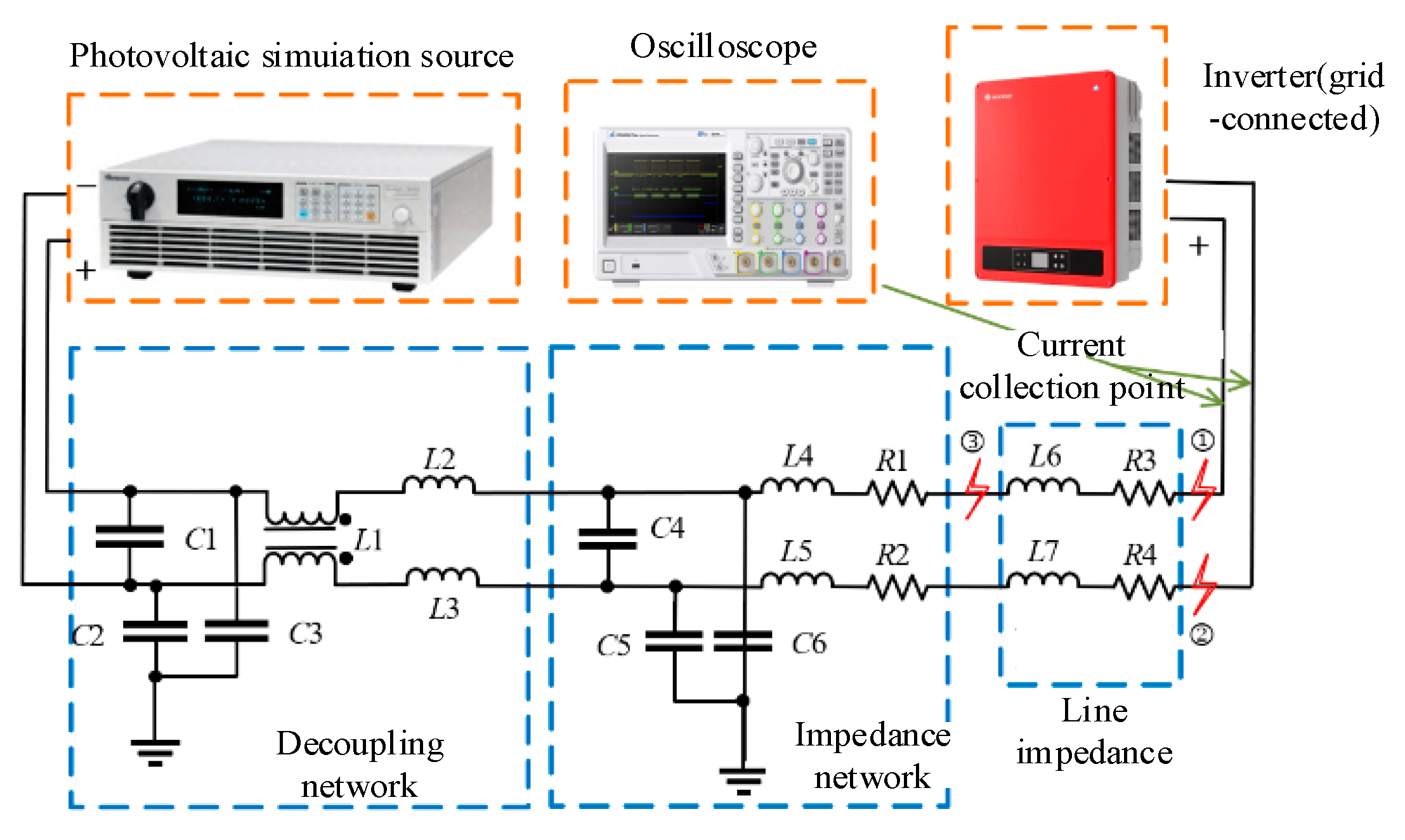
2.2. Analysis of Photovoltaic DC SAF Detection Test Scheme

For experimental analysis, this study chose a set of photovoltaic module test lines that implement inverter-integrated maximum power point tracking (MPPT) according to the UL 1699 B standard. The test platform used is depicted in Figure 3. In accordance with standard protocols, a photovoltaic simulation source was connected in series with a decoupling network and an impedance network to replicate the power generation characteristics of an actual photovoltaic panel. Arc initiation points were established at the “beginning ➀” and “end ➁” of the string. To investigate the attenuation effect of line impedance on arc signals, an additional arc initiation point ➂ was positioned upstream of the positive bus line impedance. The UL 1699 B standard specifies that the positions of arc occurrence are determined in the ‘string head’ and ‘string tail’, respectively. The attenuation effect of line impedance on the arc signal was studied by setting the arc occurrence position before the line impedance of the positive bus.

The decoupling network primarily modifies the output capacitance of the photovoltaic analog source and replicates the DC properties of the actual photovoltaic panel.

Table 3. Decoupling network element parameters.

Component	Value	Component	Value
C1	20 µF	L1	12 mH
C2	22 nF	L2	60 µH
C3	22 nF	L3	60 µH

reports the parameters of the components in the decoupling network.

A combined impedance network and photovoltaic simulation source accurately model the high-frequency properties of a photovoltaic panel when an arc is present in the natural photovoltaic system. The line impedance is a mathematical representation used to model the impedance of a parallel line. The selection of the 80 m line adheres to the UL 1699 B standard.

Table 4. Impedance network and line impedance element parameters.

Component	Value	Component	Value
C4	10 uF	R1	1 Ω
C5	1 nF	R2	1 Ω
C6	1 nF	L6, L7	0.7 µH/m
L4	50 µH	R3, R4	10 mΩ/m
L5	50 µH

displays the component parameters of the impedance network and the line impedance.

The ZDS4054 Plus oscilloscope is utilized for real-time observation and recording of the data change trend during acquisition. Given that the oscilloscope has a maximum input voltage of 300 V and the test involves a maximum voltage of 810 V, the Yokogawa 701926 high-voltage differential probe is employed for measuring the arc voltage. The Yokogawa 701933 current probe is used for current measurement in modern data acquisition. The waveform shown on the oscilloscope screen is modified throughout the test to preserve the necessary data and conduct subsequent investigations and analysis.

3. Characteristic Analysis and Model Construction of DC Fault Arc

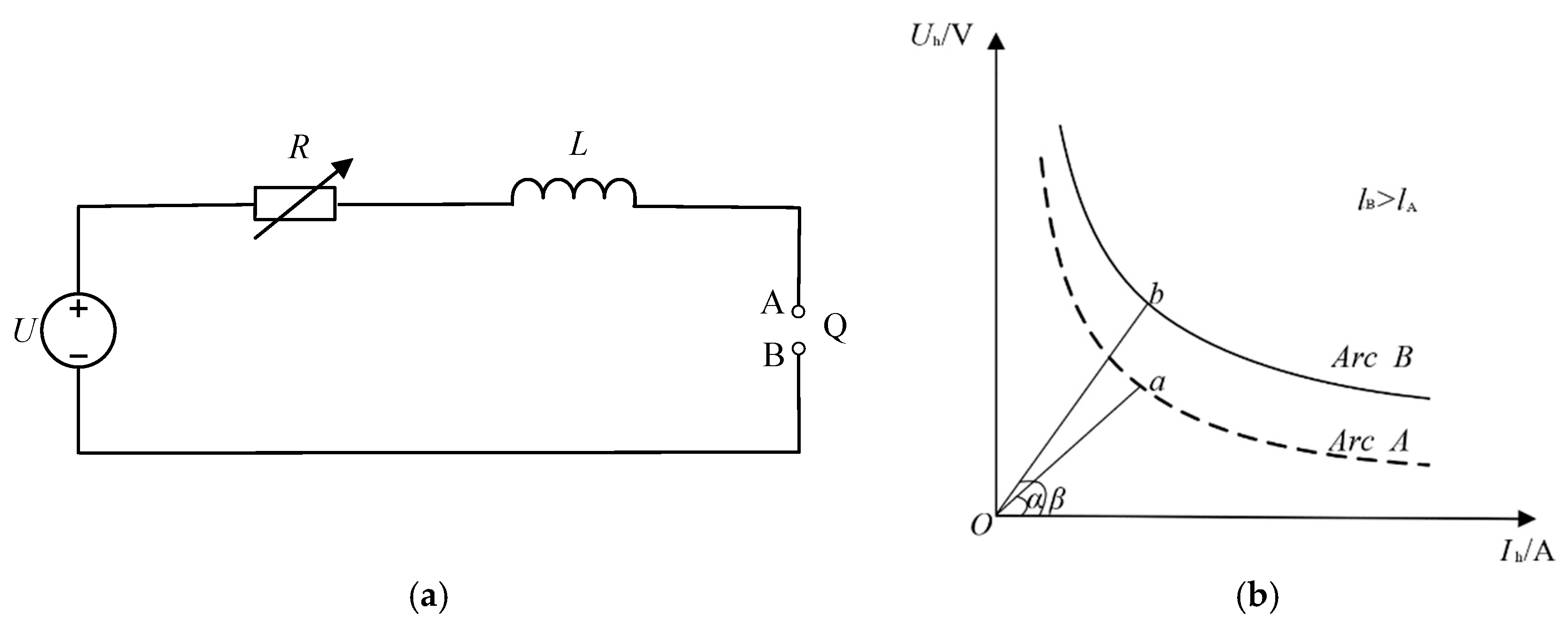
3.1. Characteristic Analysis

The DC fault arc has a cathode, anode, and arc column sections. Energy equilibrium states that the arc extinguishes when its input energy is less than its emitted energy, lowering its temperature and diameter. Consider an arc with equal input and output energy. The arc column’s temperature and diameter remain constant as it burns steadily. Consider that the arc absorbs more energy than it dissipates. Fuel combustion in the arc increases, as does arc column temperature and diameter. Energy is mainly dissipated by heat conduction, convection, and radiation in the arc.

The dynamic energy balance equation of arc can be expressed as

$${\displaystyle \frac{\mathrm{d}{\mathrm{W}}_{\mathrm{Q}}}{\mathrm{dt}}}={\mathrm{P}}_{\mathrm{h}}-{\mathrm{P}}_{\mathrm{s}}$$

(1)

In the formula, W_Q is the arc energy, t is time, P_h is the arc power, and P_s is the total output power. P_t is the heat conduction heat dissipation power, P_c is the heat convection heat dissipation power, and P_r is the heat radiation heat dissipation power. P_s = P_t + P_c + P_r. The calculation formula of heat conduction heat dissipation power P_t is

$${\mathrm{P}}_{\mathrm{t}}={\displaystyle \frac{\mathrm{k}{\mathrm{A}}_{\mathrm{t}}∆{\mathrm{T}}_{\mathrm{t}}}{\mathrm{d}}}$$

(2)

In the formula, k is thermal conductivity, A_t is the conduction heat transfer area, and d is the heat transfer distance. $∆{\mathrm{T}}_{\mathrm{t}}$ is the temperature difference between the arc and the air or electrode.

The calculation formula of thermal convection heat dissipation power is

$${\mathrm{P}}_{\mathrm{c}}=\mathrm{h}{\mathrm{A}}_{\mathrm{c}}∆{\mathrm{T}}_{\mathrm{c}}$$

(3)

In the formula, h is the convective heat transfer coefficient, A_c is the convective heat transfer area, mainly the surface area of the arc column, and $∆{\mathrm{T}}_{\mathrm{c}}$ is the temperature difference between the arc surface and the environment.

The calculation formula of thermal radiation heat dissipation power is

$${\mathrm{P}}_{\mathrm{r}}={\epsilon }_{\mathrm{r}}\sigma {\mathrm{A}}_{\mathrm{r}}{(∆{\mathrm{T}}_{\mathrm{r}})}^4$$

(4)

In the formula, ${\epsilon }_{\mathrm{r}}$ is the arc radiation coefficient, $\sigma$ is the Stefan–Boltzmann constant, A_r is the radiation heat transfer area, and $∆{\mathrm{T}}_{\mathrm{r}}$ is the temperature difference between the arc and the surrounding environment.

Arc heat dissipation relies on heat conduction and convection. Heat radiation contributes a small amount that is still significant to vacuum arc heat dissipation [22]. The MHD model developed in this work focuses on heat conduction and convection.

The arc burns freely in the air domain, and the laminar flow module is selected as the flow field. The reference pressure level is selected as an atmospheric pressure, and the reference temperature is set to 293.15 K. In the initial value setting, the speed is set to 0, the pressure is set to atmospheric pressure, and multiple physical fields share a coordinate system. The walls are set as boundaries 4 and 5 of the air domain. In the disconnection and connection loosening model, in order to produce the arcing effect, the cathode needs to move downward according to the set speed. The outlet is set as boundaries 6, 7, 8, and the pressure value is set to atmospheric pressure.

Due to the need to study the temperature change of the arc, the fluid heat transfer module is selected and the dependent variable is temperature. The fluid setting is for the air domain. Since the ‘thermal convection effect’ needs to be coupled with the laminar module, the ‘velocity field’ option needs to be selected. The heat conduction effect depends on the choice of materials. The fluid type is set as ‘gas/liquid’, and the density, constant pressure heat capacity, and specific heat rate are set as ‘from the material’. The initial temperature of the whole simulation area is set to 293.15 K. The two electrodes are set as the solid region, and the heat transfer parameters are set in the heat flux setting. The heat flux is set as ‘convective heat flux’, the external temperature is set to 293.15 K, and the heat transfer coefficient is set to W/(m²·K).

The experimental circuit for determining the static current–voltage characteristics of DC fault arcs is illustrated in Figure 4a. The circuit primarily consists of a DC power supply U, a variable resistor R, an inductor L, and an arc gap Q (where A represents the anode and B the cathode). The static current–voltage characteristic curve of the DC fault arc is obtained by measuring the voltage across the arc gap and the current flowing through it. By systematically varying the arc length and conducting repeated measurements, a family of static current–voltage characteristic curves corresponding to different arc lengths can be established. Figure 4b shows arc current I_h on the abscissa and arc voltage U_h on the ordinate. Arc voltage decreases with current, and arc resistance stabilizes on the static characteristic curve. According to static volt–ampere characteristic curves, arc resistance increases proportionally with arc length. Arcs resist current voltage and current according to the static characteristic curve’s gradient of the line connecting a point to the origin. Example: Arc resistance at point A is tanα, while at point B, it is tanβ. Multiple researchers have used mathematical fitting to derive the generic static characteristic formula under various conditions [23], as shown in

Table 5. Fitting formulas of static volt–ampere characteristics of DC arc faults.

Proposer	Fitting Formula	Test Conditions
Ayrton	UA= a + b l + (c + dl)/IA	IA < 100 A l < 10 mm
Nottingham	UA = a + b /In A	n is related to the electrode material l: 1~10 mm
Paukert	UA = a/I bA	IA: 0.3~100 kA l: 1~200 mm

. In the Table, a, b, c, and d are experimental constants, l is arc length, and I_A is arc current.

In fast current fluctuations, the dynamic volt–ampere ratio describes the arc voltage–current correlation due to thermal inertia, with arc temperature and column diameter changing slower than the current. Thus, when the current increases rapidly, the arc resistance exceeds the static volt–ampere characteristic curve resistance. The static volt–ampere characteristic curve shows a higher resistance than the arc resistance under rapid current reduction. Thus, the dynamic volt–ampere characteristic curve has several curves with different current change rates. This study examines the arc’s dynamic volt–ampere characteristics under various experimental conditions.

3.2. Arc Simulation Model Control Equation

COMSOL Multiphysics 6.0 is a simulation software suitable for multiphysics coupling. The essence of the multiphysics coupling problem is the establishment and solution of partial differential equations. As long as the model can be described by partial differential equations, COMSOL Multiphysics 6.0 software can be used to simulate and analyze it. The arc model simulation framework is shown in Figure 5.

In order to streamline computation and enhance the simulation speed, this study utilizes the r-z cylindrical coordinate system to construct a two-dimensional axisymmetric model based on the arc model, which can be considered a two-dimensional similar model. Given the assumption of a two-dimensional axisymmetric flow in the arc, the simplified equations of the arc MHD model are reformulated into Equations (5) to (11) based on the requirements of constructing the arc simulation model. The control equations are then derived by summarizing the Maxwell equations. The software calculation utilizes the control equation to address the multiphysical field coupling problem involving magnetic, electric, flow, and temperature field dynamics. The choice of boundary conditions also influences the results of the final model calculation.

The energy conservation equation is [24]

$$\begin{gathered} {\displaystyle \frac{\partial \left(\rho {\mathrm{c}}_{\mathrm{p}}\mathrm{T}\right)}{\partial \mathrm{t}}}+{\displaystyle \frac{1}{\mathrm{r}}}{\displaystyle \frac{\partial \left(\mathrm{r}\rho \psi {\mathrm{v}}_{\mathrm{r}}\right)}{\partial \mathrm{r}}}+{\displaystyle \frac{\partial \left(\rho \psi {\mathrm{v}}_{\mathrm{z}}\right)}{\partial \mathrm{z}}}={\displaystyle \frac{{\mathrm{j}}_{\mathrm{r}}^2+{\mathrm{j}}_{\mathrm{z}}^2}{\lambda }}+{\mathrm{Q}}_{\mathrm{rad}} \\ +{\displaystyle \frac{1}{\mathrm{r}}}{\displaystyle \frac{\partial \left(\frac{\mathrm{rk}}{{\mathrm{c}}_{\mathrm{p}}}\frac{\partial \psi }{\partial \mathrm{r}}\right)}{\partial \mathrm{r}}}+{\displaystyle \frac{\partial \left(\frac{\mathrm{k}}{{\mathrm{c}}_{\mathrm{p}}}\frac{\partial \psi }{\partial \mathrm{z}}\right)}{\partial \mathrm{z}}}+{\displaystyle \frac{5{\mathrm{k}}_{\mathrm{B}}}{2\mathrm{e}}}\left({\mathrm{j}}_{\mathrm{r}}{\displaystyle \frac{\partial \mathrm{T}}{\partial \mathrm{r}}}+{\mathrm{j}}_{\mathrm{z}}{\displaystyle \frac{\partial \mathrm{T}}{\partial \mathrm{z}}}\right) \end{gathered}$$

(5)

where r is the radial distance, z is the axial distance, $\rho$ is the plasma density, k is the thermal conductivity, v_r is the radial velocity, v_z is the axial velocity, j_z is the radial current density, j_r is the axial current density, t is temperature, k_B is the Boltzmann constant, c_p is the heat capacity of the arc under normal pressure, ${\mathrm{Q}}_{\mathrm{rad}}$ is the total volume radiation coefficient, ‘$\psi$’ is the surface heat transfer coefficient, and e is the basic charge.

The radial momentum conservation equation is

$$\begin{gathered} {\displaystyle \frac{\partial \left(\rho {\mathrm{v}}_{\mathrm{r}}\right)}{\partial \mathrm{t}}}+{\displaystyle \frac{1}{\mathrm{r}}}{\displaystyle \frac{\partial \left(\mathrm{r}\rho {\mathrm{v}}_{\mathrm{r}}^2\right)}{\partial \mathrm{r}}}+{\displaystyle \frac{\partial \left(\rho {\mathrm{v}}_{\mathrm{r}}{\mathrm{v}}_{\mathrm{z}}\right)}{\partial \mathrm{z}}}=-{\displaystyle \frac{\partial \mathrm{P}}{\partial \mathrm{r}}}-{\mathrm{j}}_{\mathrm{z}}{\mathrm{B}}_{\theta } \\ +{\displaystyle \frac{1}{\mathrm{r}}}{\displaystyle \frac{\partial \left(2\mathrm{r}\eta \frac{\partial {\mathrm{v}}_{\mathrm{r}}}{\partial \mathrm{r}}\right)}{\partial \mathrm{r}}}+{\displaystyle \frac{\partial \left[\eta \left(\frac{\partial {\mathrm{v}}_{\mathrm{r}}}{\partial \mathrm{z}}+\frac{\partial {\mathrm{v}}_{\mathrm{z}}}{\partial \mathrm{r}}\right)\right]}{\partial \mathrm{z}}}-2\eta {\displaystyle \frac{{\mathrm{v}}_{\mathrm{r}}}{{\mathrm{r}}^2}} \end{gathered}$$

(6)

The axial momentum conservation equation is

$$\begin{gathered} {\displaystyle \frac{\partial \left(\rho {\mathrm{v}}_{\mathrm{z}}\right)}{\partial \mathrm{t}}}+{\displaystyle \frac{1}{\mathrm{r}}}{\displaystyle \frac{\partial \left(\mathrm{r}\rho {\mathrm{v}}_{\mathrm{r}}{\mathrm{v}}_{\mathrm{z}}\right)}{\partial \mathrm{r}}}+{\displaystyle \frac{\partial \left(\rho {\mathrm{v}}_{\mathrm{z}}^2\right)}{\partial \mathrm{z}}}=-{\displaystyle \frac{\partial \mathrm{P}}{\partial \mathrm{z}}}+{\mathrm{j}}_{\mathrm{r}}{\mathrm{B}}_{\theta } \\ +{\displaystyle \frac{\partial \left(2\eta \frac{\partial {\mathrm{v}}_{\mathrm{r}}}{\partial \mathrm{z}}\right)}{\partial \mathrm{z}}}+{\displaystyle \frac{1}{\mathrm{r}}}{\displaystyle \frac{\partial \left[\mathrm{r}\eta \frac{\partial {\mathrm{v}}_{\mathrm{r}}}{\partial \mathrm{z}}+\frac{\partial {\mathrm{v}}_{\mathrm{z}}}{\partial \mathrm{r}}\right]}{\partial \mathrm{r}}} \end{gathered}$$

(7)

In the formula, P is the plasma pressure, “j_r”, “B_θ”, and “j_z” “B_θ” are Lorentz forces, and “η” is the dynamic viscosity coefficient.

The current continuity equation is

$${\displaystyle \frac{1}{\mathrm{r}}}+{\displaystyle \frac{\partial \mathrm{r}\psi \frac{\partial \mathrm{V}}{\partial \mathrm{r}}}{\partial \mathrm{r}}}+{\displaystyle \frac{\partial \left(\psi \frac{\partial \mathrm{V}}{\partial \mathrm{z}}\right)}{\partial \mathrm{z}}}=0$$

(8)

In the formula, V is the potential.

The mass conservation equation is

$${\displaystyle \frac{\partial \rho }{\partial \mathrm{t}}}+{\displaystyle \frac{1}{\mathrm{r}}}{\displaystyle \frac{\partial \left(\mathrm{r}\rho {\mathrm{v}}_{\mathrm{r}}\right)}{\partial \mathrm{r}}}+{\displaystyle \frac{\partial \left(\rho {\mathrm{v}}_{\mathrm{z}}\right)}{\partial \mathrm{z}}}=0$$

(9)

Maxwell ’s equation is

$${\displaystyle \frac{1}{\mathrm{r}}}{\displaystyle \frac{\partial \left(\mathrm{r}{\mathrm{B}}_{\theta }\right)}{\partial \mathrm{r}}}={\mathrm{j}}_{\mathrm{z}}{\mathrm{\mu }}_0$$

(10)

In the formula, “μ₀” is the vacuum permeability.

The expression of Ohm’s law is

$$\begin{gathered} {\mathrm{j}}_{\mathrm{r}}=-\lambda {\displaystyle \frac{\partial \mathrm{V}}{\partial \mathrm{r}}} \\ {\mathrm{j}}_{\mathrm{z}}=-\lambda {\displaystyle \frac{\partial \mathrm{V}}{\partial \mathrm{z}}} \end{gathered}$$

(11)

In the formula, “λ” is conductivity.

To simplify arc simulation and expedite model convergence, the following assumptions are specified based on References [25,26,27,28]:

(1)

The arcing stage is not considered;

(2)

The burning of the two electrodes by the arc and the sheath in the near-polar region is ignored;

(3)

The arc is treated as an incompressible fluid;

(4)

The arc is axisymmetric, and the flow of the arc fluid is laminar in the case of free arcing;

(5)

The arc’s thermodynamic properties vary with temperature, including density, thermal conductivity, constant pressure heat capacity, and viscosity coefficient.

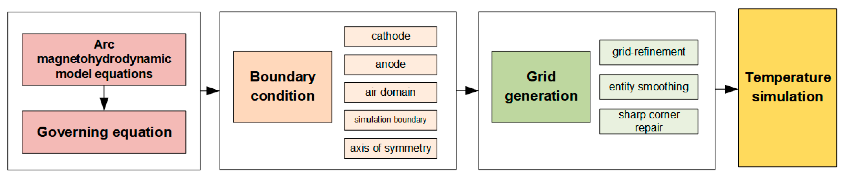
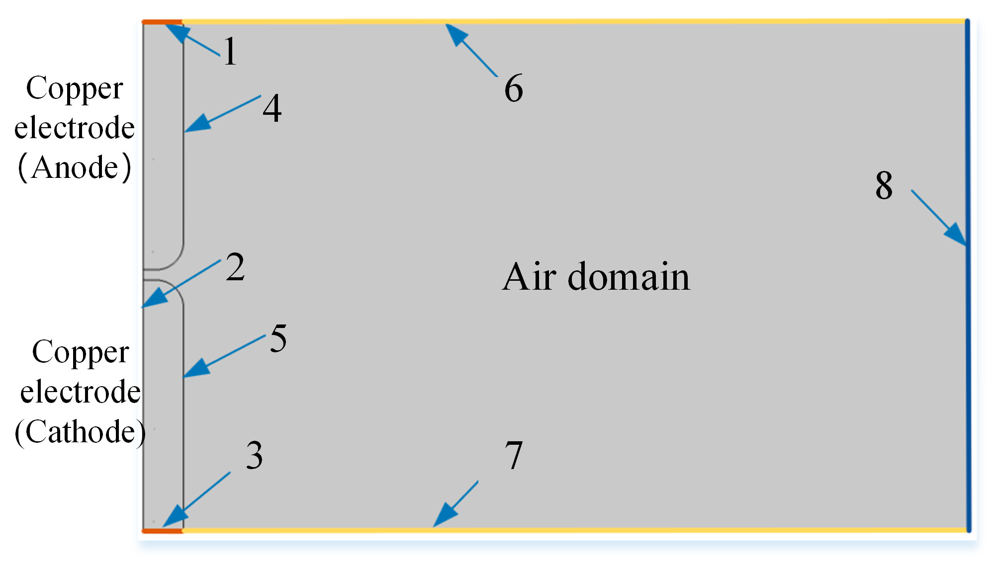
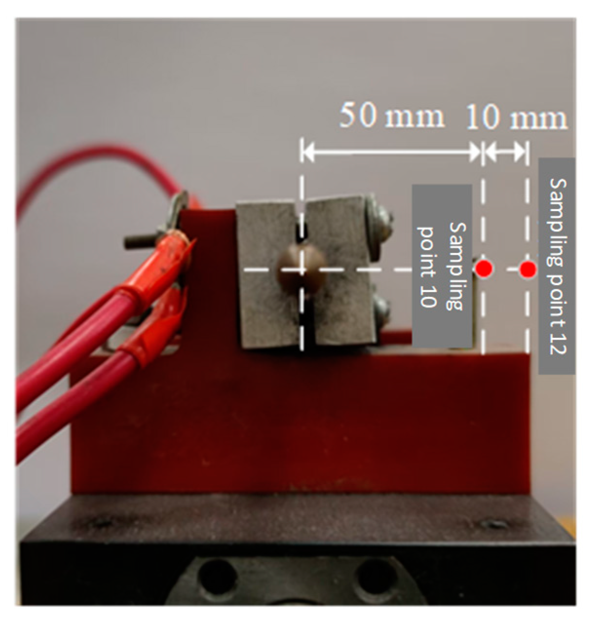
3.3. Fault Arc Boundary Conditions and Mesh Generation

This work presents an arc model with five modules: current, magnetic field, flow field, fluid heat transfer, and circuit, which are used to build the MHD model according to the construction criteria. Flow and temperature coupling are achieved using multiphysical field coupling for arc temperature simulations. Figure 6 shows numerical references for model region boundaries. boundary 1 is the external circuit-integrated anode and current inlet. Current flow stops at boundary 3, the obscured outermost section connected to the external circuit. The symmetry axis is boundary 2. The linear axis of symmetry will be symmetrically processed after simulation. In the actual scenario, the cathode and anode will have a diameter of 6.35 mm and air domains on both sides. The anode, cathode, and air domains intersect at boundaries 4 and 5. The simulation’s upper, lower, and proper boundaries are 6, 7, and 8.

Arc fault model research focuses on the electrode–air domain junction and arc gap. These two locations require a more complicated grid design than the others. Unit size mesh generation of the air domain uses a predefined refinement grid for fluid dynamics calibration. The unit size is calibrated to fluid dynamics standards for air domain–electrode interface boundaries 4 and 5. A predetermined ultra-thin mesh is used. Air domain and boundary points 4 and 5 undergo angle refinement iterations. The refinement unit-size scaling factor is 0.25, and the minimum boundary angle is 240°. The rest is divided by an autonomous triangle. A 1-scale ratio is used for geometric scaling across the region. The ’cross-removed control entity is smoothed’ setting is used with eight iterations and 8-unit depths. Due to the coarse remaining area, automatic refinement is chosen.

The gap breakdown model focuses primarily on the arc gap and the electrode–air domain interface, necessitating a more refined mesh in these regions while maintaining relatively coarse discretization elsewhere. For the air domain, a predefined refined mesh was implemented. At the interfaces between the air domain and the two electrodes (boundaries 4 and 5), a predefined ultra-fine mesh was applied. Additional angle refinement was performed on both the air domain and boundaries 4 and 5, while the remaining regions were discretized using free triangular elements. In the scaling geometry operation, the entire domain was assigned a scale factor of 1, with eight iterations and a maximum element depth of 8. For regions requiring less resolution, an automatic refinement method was selected. Subsequently, a boundary layer mesh was applied to further refine boundaries 4 and 5, with sharp corners trimmed to improve mesh quality. The boundary layer configuration consisted of two layers with a stretching factor of 1.2 and a thickness adjustment factor of 5. Conventional refinement was applied to the arc gap region. The resulting mesh structure is illustrated in Figure 7.

4. Experimental Verification and Fire Risk Analysis

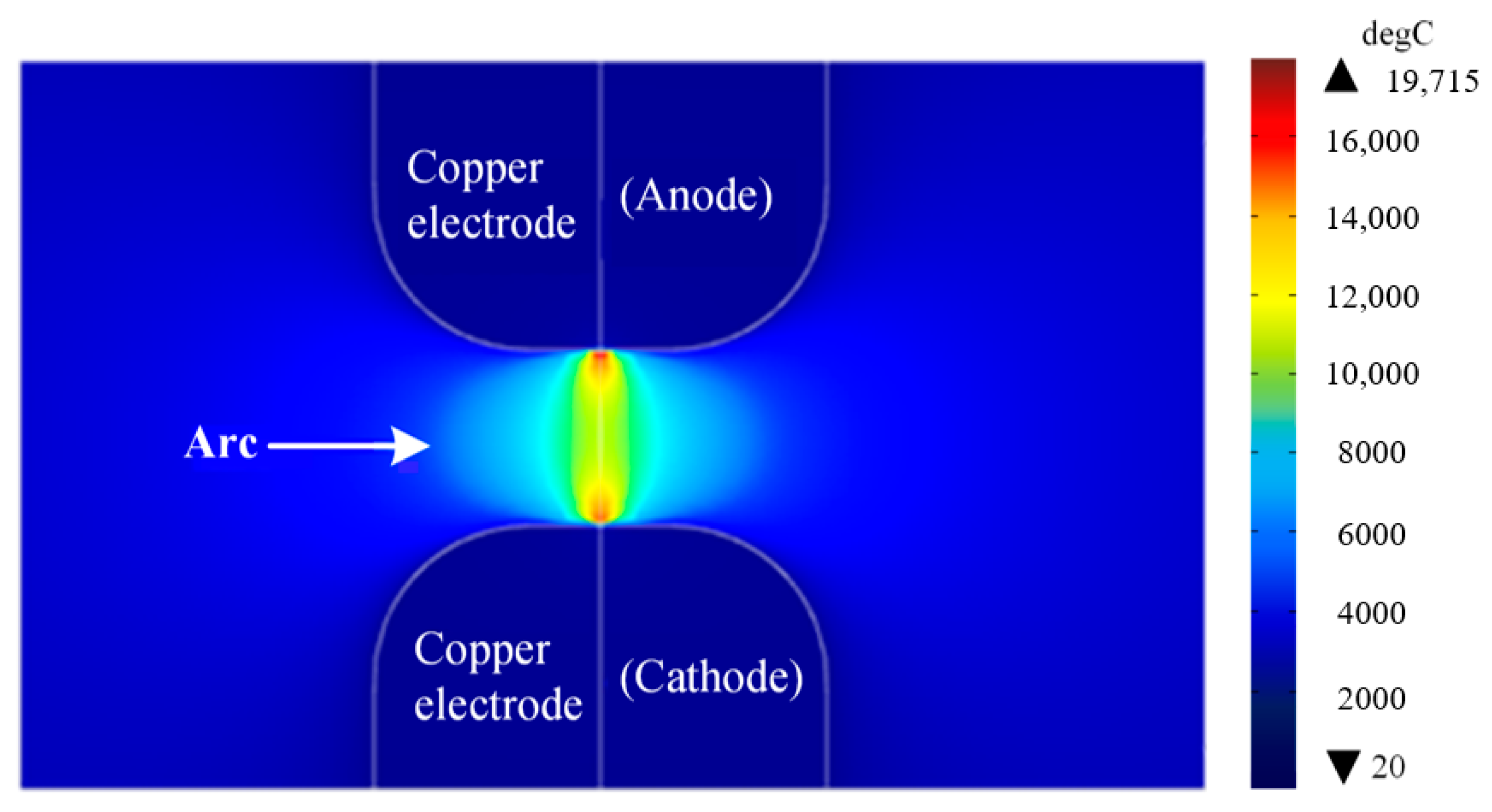
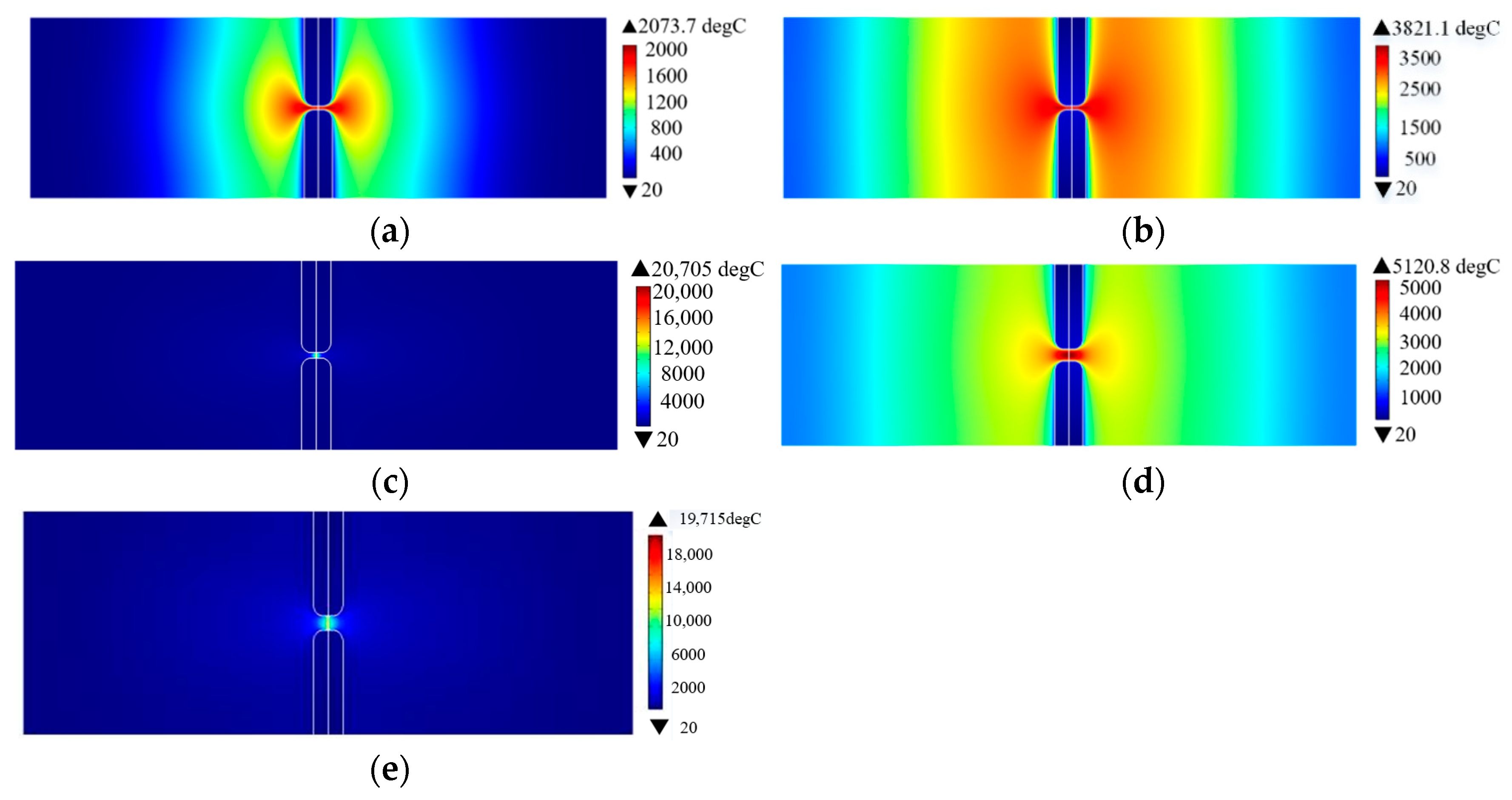
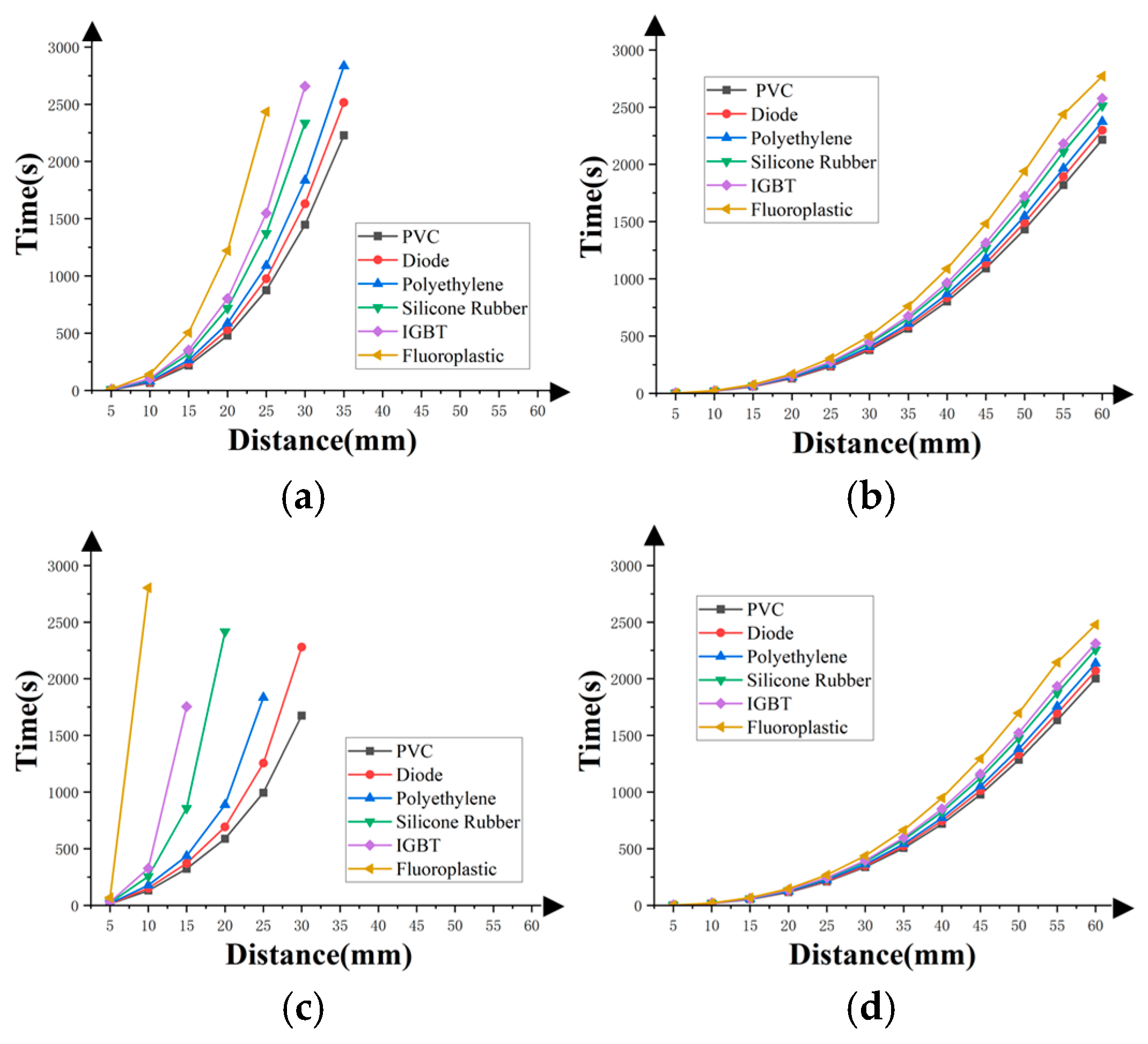
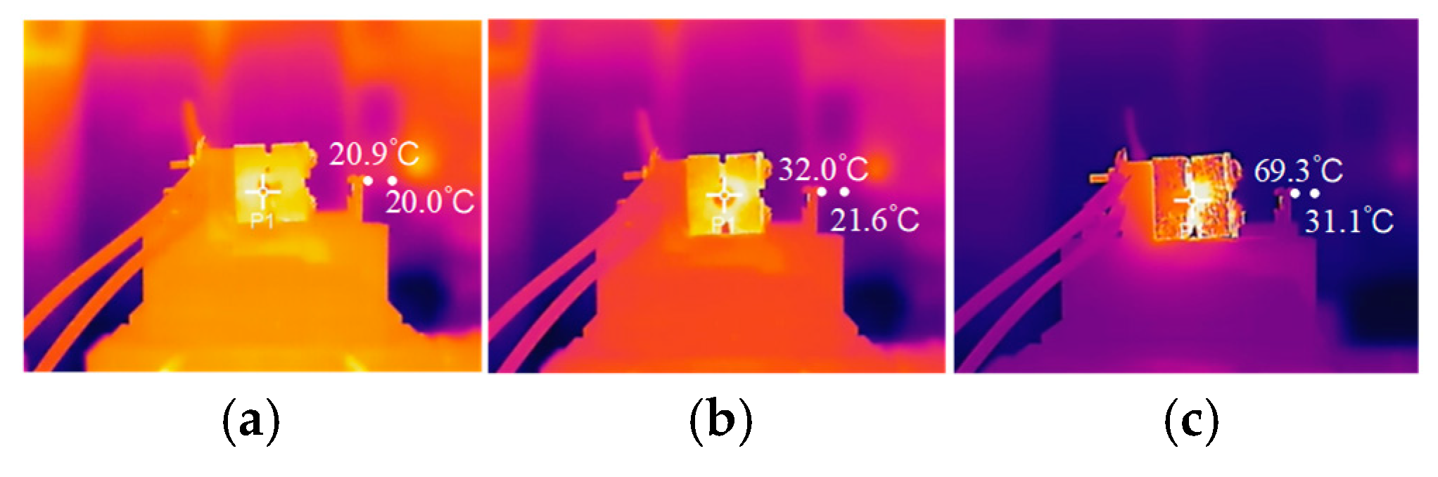
4.1. Arc Gap Temperature Change Rule

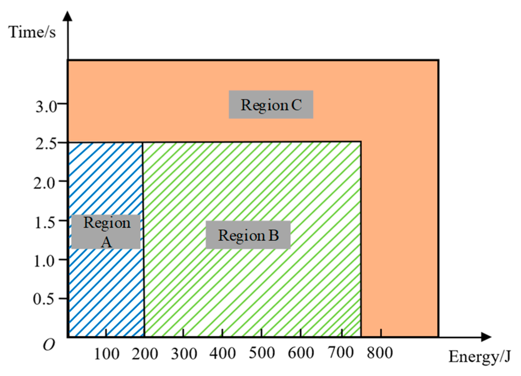
According to our simulations, the arc temperature stops rising after 3 s. Thus, under maximum current of 25, the fault arc model simulation results are obtained at 3 s. Figure 8 accurately depicts arc temperature distribution under test conditions. The arc contact electrode’s arc root has the highest temperature and causes material loss from electrode burning. The central temperature of the arc column is higher than that of the outer layer, but it decreases as the distance from it increases.

The fault arc model’s arc gap is predetermined based on the information presented in Table 2. At a sufficient voltage, the arc gap disintegrates, forming an arc. The simulation shows that the arc temperature stops rising after 3 s. Thus, the 3-s simulation results are examined. Figure 9a–d shows the arc gap temperature distribution for tests 1–4 conditions. Figure 9c shows that air molecules collide more often and more intensely when the arc gap temperature is too high. These motions and collisions accelerate heat transfer. Therefore, when the arc gap temperature is too high, the nearby air is more likely to transmit heat to the surrounding environment, increasing heat dissipation. The arc gap temperature rises while the ambient air temperature falls, resulting in a blue hue. Using the conditions of tests 1–4 from Table 2 and the arcing durations of 0.5 s, 1.0 s, 1.5 s, 2.0 s, 2.5 s, and 3.0 s,

Table 6. The variation law of arc fault gap temperature with time in the gap breakdown model.

Item	Max Arc Temperature at Different Times/°C
	0.5 s	1.0 s	1.5 s	2.0 s	2.5 s	3.0 s
1	2065	2068	2070	2072	2073	2073
2	3814	3817	3818	3820	3820	3821
3	21,001	20,901	20,837	20,784	20,735	20,705
4	5210	5174	5152	5138	5129	5120

shows the resulting maximum arc gap temperatures. This table directly shows arc gap temperature variation over time. The elevated temperatures of the arc gap tend to ignite nearby combustibles. The phenomenon is thoroughly examined in Section 4.2.

Figure 9 shows the simulation results of the temperature distribution of the arc gap when the arcing time is 3.0 s under the different conditions; the maximum temperature can reach 2073 °C, 3821 °C, 20,705 °C, 5120 °C, and 19,715 °C. Analysis of the information presented in Figure 9 and Table 6 reveals that the arc gap size of test 1 and test 2 is the same, the power supply voltage is relatively similar, the line current of test 2 is approximately 2.67 times greater than that of test 1—its arc gap temperature is around 1800 °C higher than that of test 1. The temperature of the arc gap is directly proportional to the arc current. The power supply voltages of test 2 and test 3 exhibit consistency, while the arc gap shows minimal variation. For test 3, the line current is double that of test 2, and the temperature is approximately 5.4 times higher than that of test 2. The present size is the determining factor in arc temperature. The difference in current between test 2 and test 4 is negligible. The power supply voltage of test 4 is approximately 1.9 times higher than that of test 2, while the arc gap is 3.125 times greater than that of test 2. Despite the larger arc gap of test 4, its voltage is also greater, thus amplifying the significance of the arc gap energy. Therefore, the breakdown of the arc gap is more direct, leading to the higher temperature exhibited by test 4 compared to test 2.

According to the analysis provided, the variability of the arc gap temperature in the arc fault model is influenced by several parameters including line current, power supply voltage, and arc gap size. Nevertheless, the line current exerts the most substantial impact on the temperature of the arc gap. The arc gap temperature increases proportionally with the magnitude of the current. The impact of arc gap size and power supply voltage on arc gap temperature is comparatively smaller than that of current saturation. More significant arc gaps correspond to lower temperatures. Increased power supply voltage corresponds to increased temperature.

4.2. Risk Analysis

Based on the study of temperature characteristics and development and influencing factors, we provide

Table 7. Summary of the mechanism of arc fire disaster.

I/A	U/V	Gap/mm	Max Arc Temperature at Different Times/°C			Analysis
			0.5 s	1.5 s	2.5 s
3	312	0.8	2065	2070	2073	With the increase in voltage and current, the temperature of sampling point rises faster, and the risk of arc ignition rises rapidly. The increase in arc gap size limits the temperature rise speed and reduces the fire risk to a certain extent.
8	318	0.8	3814	3818	3820
16	318	1.1	21,001	20,837	20,735
8.5	607	2.5	5210	5152	5129.3

to summarize the mechanism of arc fire occurrence, as follows. The UL 1699B standard requires interrupting the circuit within 2.5 s of arc detection to prevent fires. Using the conditions of tests 1–4 shown in Table 2, the fault arc model is used to study the arc gap’s maximum temperature change curve and temperature distribution pattern. The simulation lasts 3 s, with 0.1 ms steps. The temperature change law of the arc after 3 s is unimportant for arc ignition risk assessment. Self-heating spontaneous combustion and carbonization are two types of spontaneous combustion. High arc temperatures warm atmospheric air through heat conduction, convection, and radiation. Arc temperature reaches the ignition point without direct contact with combustibles. When heated, flammables spontaneously burn, starting fires. Thus, the arc’s temperature fluctuation regime must be examined.

To investigate the fire risk posed by electric arcs to surrounding combustible materials, 12 temperature sampling points were positioned adjacent to the arc gap in the arc model (at distances of 5, 10, 15, 20, 25, 30, 35, 40, 45, 50, 55, and 60 mm from the arc gap center). Temperature profiles at these points were analyzed to evaluate the thermal impact of the arc on proximate combustible materials. Combustible components in photovoltaic systems typically include wire insulation and power electronic devices within inverters. If an electric arc heats the surrounding air to the ignition temperature of these materials, there exists a risk of spontaneous combustion due to thermal exposure. Consequently, arc detection and circuit interruption must occur before the temperature at combustible material locations reaches the ignition threshold to prevent fire incidents. Wire insulation materials commonly include polyvinyl chloride (ignition temperature: 250 °C), polyethylene (ignition temperature: 350 °C), silicone rubber (ignition temperature: 450 °C), and fluoroplastics (ignition temperature: 670 °C). Power electronic components typically include diodes (ignition temperature: 300 °C) and IGBTs (ignition temperature: approximately 500 °C). It should be noted that these ignition temperatures represent standard conditions; actual ignition thresholds may vary depending on manufacturing processes and operational conditions. To comprehensively characterize the temporal–thermal relationship in the vicinity of the arc gap, this study analyzes the time required for different sampling points to reach the ignition temperatures of the aforementioned combustible materials within a 3-s interval.

The temperature flux of these 12 locations was analyzed to determine how Figure 10a shows the time at which each sampling point reaches the ignition point of the combustible under test 1 conditions, with a line current of 3.0 A, a power supply voltage of 312 V, and an arc gap of 0.8 mm. Significantly, the ignition point will be at most 35 mm from the sampling point. The temperature rises faster as the temperature sampling point approaches the arc gap (Figure 10a). This accelerates the ignition point of the combustible material, significantly increasing fire risk. However, extinguishing the arc takes time due to the photovoltaic system’s component distances. A fire can be prevented by extinguishing the arc before the sampling point at the matching location reaches the fuel ignition point.

Figure 10b shows when sampling points 1–12 reach the ignition point of each combustible under test 2 conditions: 8.0 A line current, 318 V power supply voltage, and a 0.8 mm arc gap. Figure 10a,b shows that when the power supply voltage and arc gap size are nearly equal, the sampling point temperature reaches the ignition point of combustibles faster as the line current increases. This phenomenon increases line-cutting speed requirements.

Figure 10c shows that in test 3, with a line current of 16.0 A, a power supply voltage of 318 V, and an arc gap of 1.1 mm, the time sampling points 1–12 reach each fuel’s ignition point. Temperature will not exceed ignition point beyond 35 mm from the sampling point. While maintaining a constant power supply voltage, the arc temperature increases as the arc gap size increases. Figure 10c shows that the time to reach the fuel’s ignition point increases. The main reason is that arc gap size increases and complicates arc breakdown, preventing arc development. Thus, increasing the arc gap reduces arc ignition occurrences.

Figure 10d shows the time at which sampling points 1–12 reach the ignition point of each combustible in under test 4 conditions, with an 8.5 A line current, a 607 V power supply voltage, and a 2.5 mm arc gap. Figure 10b,d shows that test 4’s power supply voltage is 1.9 times that of test 2. The arc gap size in test 4 is 3.125 times more significant than that of test 2, assuming constant line current. Thus, test 4 has a higher temperature rise rate at each sampling point than test 2. For larger power supply voltages, the rate of temperature increase around the arc accelerates, and the power supply voltage affects temperature more than the arc gap size.

4.3. Risk Validation

Heat transfer from the arc gap to the air becomes more challenging as the distance from it increases. The size of the arc-generating device determines the verification sampling locations at 50 and 60 mm from the arc gap. If the arcing time is 1, 2, or 3 s, the thermal imager’s continuous shooting mode can accurately measure the sampling point’s temperature with a minimum interval of 1 s. The photo shown in Figure 11 was obtained using the photo mode of an HIKMICRO H36. Figure 10 shows the necessary proof of temperature sampling points 10 and 12. The slider is secured by a screw that is not aligned with the arc gap. The infrared thermal image shows the temperature peak along a straight line perpendicular to the lens. The test begins when the central air conditioner sets the room temperature to 20 °C, the simulation model’s starting temperature.

Based on the temperature simulation results at sampling points 10 and 12 within a 3-s timeframe for test items 1 to 4, as presented in

Table 8. Temperature simulation values of temperature sampling point 10.

Time	Max Arc Temperature at Different Times/°C
	1	2	3	4
1 s	20.9	45.5	20.3	66.2
2 s	32.1	713.3	32.9	922.4
3 s	69.5	1315.5	66.7	1664

and

Table 9. Temperature simulation values of temperature sampling point 12.

Time	Max Arc Temperature at Different Times/°C
	1	2	3	4
1 s	20	21.4	19.9	21.8
2 s	21.6	144.9	21.3	248.5
3 s	31.1	906.0	30.8	1344.9

, the temperatures at sampling points 10 and 12 are below 650 °C, within the infrared thermal imager temperature range. This finding can be confirmed by experimental verification.

The images shown in Figure 12 and Figure 13 were obtained using the infrared mode of an HIKMICRO H36. Figure 12 shows infrared thermal images of temperature sampling points 10 and 12 at 1 s, 2 s, and 3 s under test 1 conditions. The P1 point is adjusted to align the copper rod for shot measurements to ensure a uniform shooting range for each image. The matching processing software of the infrared thermal imager can only display the mouse cursor temperature at any given time, not sampling points 10 and 12. Thus, temperature data is directly displayed and annotated in the same image, ensuring precise test results. Comparing the recorded temperature value to Table 9 and

Table 10. Results comparison of the proposed model with prior models.

Particulars	Yan. et al. [29]	Yang et al. [30]	Hu et al. [31]	Wu et al. [15]	This Paper
Model used	Cassie arc model	Mayr arc model	Mayr-Cassie arc model	MHD model	MHD model
Voltage and current	Yes	Yes	Yes	Yes	Yes
Arc gap size	No	No	No	Yes	Yes
Heat transfer	No	No	No	Yes	Yes
Temperature-time characteristics	No	No	No	Yes	Yes
Complexity	Simple	Simple	Medium	Complex	Complex

, the simulation data show a maximum deviation of 0.31% from the test results. This means the simulation results are trustworthy.

Figure 13 displays the infrared thermal images of temperature sampling points 10 and 12 at 1-s, 2-s, and 3-s intervals under test 3 conditions. The recorded temperature values are contrasted with those obtained from model calculations in Table 9 and Table 10. The maximum discrepancy between the simulation results and the test results is 0.32%, rendering the simulation results reliable.

At the same time, the DC arc model based on MHD used in this paper is compared with other models, as shown in Table 10. The existing models can simulate the voltage and current, but the Cassie and Mayr models cannot simulate the arc gap size, heat conduction, and time-temperature characteristics. However, the model based on MHD can simulate the arc gap size, heat conduction, and other aspects. The MHD model used in the other literature does not consider the time–temperature characteristics. Our model considers these aspects and can effectively support the development needs of photovoltaic systems. However, the calculation of this method is more complicated, and the requirements for the computing platform are higher.

5. Discussion

In this paper, an MHD arc fault simulation model that takes into account multiple physical fields has been developed. The study investigates the time–temperature characteristics of photovoltaic DC arc faults under various operating conditions. It reveals how factors such as line current, power supply voltage, and arc gap size influence the maximum temperature of the arc. The findings indicate that the current level is the most critical factor affecting arc temperature, followed by the power supply voltage and the size of the arc gap. The variation law of arc fault temperature with time was studied, and the time required for the external temperature of arc fault to reach the ignition point of surrounding combustibles under different current levels was obtained, which effectively characterizes the risk of arc fault ignition. The arc temperature experiment was designed to verify the accuracy of the model—the fault arc’s temperature changes at 5 cm and 6 cm under different working conditions. The error of the model simulation’s accuracy is within 0.31%, and the model’s reliability is thus proven. This study clarifies the influencing factors of arc fault temperature and the range of ignition risk, which provides strong support for evaluating the arc fault risk level and the electrical safety design of the photovoltaic power generation system.

The simulation model in this paper does not consider the influence of the thermal conductivity of various ignition materials on the ignition factors of arc faults in a complex environment. Based on the arc fault simulation model and ignition law proposed in this paper, future research can establish a scientific optimization scheme considering the heat capacity and thermal conductivity parameters of the arc fault simulation model material in a complex environment.

References

1. Wang, Y.; Zhang, Y.; Li, K. A review of research on photovoltaic DC arc fault detection methods. Electr. Appl. Energy Effic. Manag. Technol. 2018, 561, 1–6+37. [Google Scholar]
2. Huang, X.; Wu, C.; Li, Z.; Wang, F. Comparative study of DC arc fault detection methods in photovoltaic systems. Acta Energiae Solaris Sin. 2020, 41, 204–214. [Google Scholar]
3. Qu, N.; Wang, J.; Liu, J. An Arc Fault Detection Method Based on Current Amplitude Spectrum and Sparse Representation. IEEE Trans. Instrum. Meas. 2019, 68, 3785–3792. [Google Scholar] [CrossRef]
4. Zou, G.; Fu, G.; Han, B.; Wang, W.; Liu, C. Series Arc Fault Detection Based on Dual Filtering Feature Selection and Improved Hierarchical Clustering Sensitive Component Selection. IEEE Sens. J. 2023, 23, 6050–6060. [Google Scholar] [CrossRef]
5. Ahmadi, M.; Samet, H.; Ghanbari, T. Series Arc Fault Detection in Photovoltaic Systems Based on Signal to Noise Ratio Characteristics Using Cross-Correlation Function. IEEE Trans. Ind. Inform. 2019, 16, 3198–3209. [Google Scholar] [CrossRef]
6. Zhai, G.; Zhou, X.; Yang, W. Arc characteristics test when disconnecting DC inductive load under longitudinal and transverse magnetic fields. Trans. Chin. Soc. Electrotech. Eng. 2011, 26, 68–74. [Google Scholar]
7. Wang, H. Simulation Study on the Influence of Multiple Physical Factors on Arc and Electrical Erosion of DC Contactor. Bachelor’s Thesis, Shenyang University of Technology, Shenyang, China, 2020; pp. 3–7. [Google Scholar]
8. Cui, Y. Arc Characteristics and Simulation Research in DC Vacuum Circuit Breaker Under Transverse Magnetic Field. Bachelor’s Thesis, Hebei University of Technology, Tianjin, China, 2017; pp. 4–5. [Google Scholar]
9. Xu, W.; Yao, L.; Qi, J.; Tian, S.; Zhang, X.; Pan, M.; Wu, X. Extraction of Fault Characteristic Frequency Band of Photovoltaic DC Series Arc Based on Wavelet Packet Transform and Tsallis Entropy. In Proceedings of the 2023 5th Asia Energy and Electrical Engineering Symposium (AEEES), Chengdu, China, 23–26 March 2023; pp. 551–558. [Google Scholar]
10. Blažič, A.; Škrjanc, I.; Logar, V. Arc Quality Index Based on Three-Phase Cassie–Mayr Electric Arc Model of Electric Arc Furnace. Metals 2024, 14, 338. [Google Scholar] [CrossRef]
11. Hashemi, E.; Niayesh, K. DC Current Interruption Based on Vacuum Arc Impacted by Ultra-Fast Transverse Magnetic Field. Energies 2020, 13, 4644. [Google Scholar] [CrossRef]
12. Jadidian, J. A Compact Design for High Voltage Direct Current Circuit Breaker. IEEE Trans. Plasma Sci. 2009, 37, 1084–1091. [Google Scholar] [CrossRef]
13. Huang, K.; Niu, C.; Wu, Y.; Rong, M.; Yang, F.; Sun, H. Arc Plasma Simulation Method in DC Relay with Contact Opening Process. In Proceedings of the 2019 5th International Conference on Electric Power Equipment-Switching Technology (ICEPE-ST), Kitakyushu, Japan, 13–16 October 2019; IEEE: Piscataway, NJ, USA, 2019; pp. 226–229. [Google Scholar]
14. Jia, B.; Wu, J.; Li, S.; Wu, H.; Peng, X.; Dai, J.; Chen, R. Magneto-hydrodynamic simulation study of direct current multi-contact circuit breaker for equalizing breaking arc. Plasma Sci. Technol. 2023, 25, 025506. [Google Scholar] [CrossRef]
15. Wu, Q.; Liu, S.; Lv, Y.; Hu, D.; Liu, Y.; Feng, B.; Hou, S.; Fu, M. Simulation Study on Steady-State Heat Transfer characteristics of DC Arc Fault. Trans. China Electrotech. Soc. 2021, 36, 2697–2709. [Google Scholar]
16. Wu, Z.; Hu, Y.; Wen, J.X.; Zhou, F.; Ye, X. A Review for Solar Panel Fire Accident Prevention in Large-Scale PV Applications. IEEE Access 2020, 8, 132466–132480. [Google Scholar] [CrossRef]
17. Wang, Y.; Wang, S.; Zhao, Q.; Zhang, W. Modelling and calculation method of minimum safety distance for photovoltaic fire extinguishing under energized conditions. Sol. Energy 2025, 288, 113300. [Google Scholar] [CrossRef]
18. Zhang, X.; Reda, I.; Aram, M.; Qi, D.; Wang, L.L.; Fellouah, H. Wind-driven smoke dispersion in rooftop photovoltaic fires: An experimental investigation with helium smoke. J. Build. Eng. 2024, 83, 108467. [Google Scholar] [CrossRef]
19. Georgijevic, N.L.; Jankovic, M.V.; Srdic, S.; Radakovic, Z. The Detection of Series Arc Fault in Photovoltaic Systems Based on the Arc Current Entropy. IEEE Trans. Power Electron. 2016, 31, 5917–5930. [Google Scholar] [CrossRef]
20. Weng, J.; Zhang, J.; Li, D.; Zheng, H. Review of anti-interference technology for DC arc fault detection in photovoltaic systems. J. Electr. Eng. 2019, 14, 9–15. [Google Scholar]
21. Kavi, M.; Mishra, Y.; Vilathgamuwa, M. DC Arc Fault Detection For Grid-Connected Large-Scale Photovoltaic Systems. IEEE J. Photovolt. 2020, 10, 1489–1502. [Google Scholar] [CrossRef]
22. Gammon, T.; Lee, W.J.; Zhang, Z.; Johnson, B.C. A Review of Commonly Used DC Arc Models. IEEE Trans. Ind. Appl. 2015, 51, 1398–1407. [Google Scholar] [CrossRef]
23. Li, Y.; Zhang, R.; Yang, K.; Qi, Y.; Tu, R. Numerical investigations of AC arcs thermal characteristics in the short gap of copper-cored wires. Sci. Rep. 2024, 14, 4227. [Google Scholar] [CrossRef]
24. Yin, F.; Hu, S.; Gao, Z. Research progress in numerical simulation of plasma arc. Ordnance Mater. Sci. Eng. 2007, 30, 59–63. [Google Scholar]
25. Bauchire, J.M.; Gonzalez, J.J.; Gleizes, A. Modeling of a DC Plasma Torch in Laminar and Turbulent Flow. Plasma Chem. Plasma Process. 1997, 17, 409–432. [Google Scholar] [CrossRef]
26. Matthaeus, W.H.; Brown, M.R. Nearly incompressible magnetohydrodynamics at low Mach number. Phys. Fluids 1988, 31, 3634–3644. [Google Scholar] [CrossRef]
27. Yin, F.; Hu, S.; Zheng, Z.; Ma, L. Numerical simulation of plasma arc welding arc. J. Weld. 2006, 27, 51–54+115. [Google Scholar]
28. Zhong, Y. MHD Model Simulation and Experimental Study of Low Current DC Air Arc. Master’s Thesis, Chongqing University, Chongqing, China, 2020; pp. 15–17. [Google Scholar]
29. Yan, K.; Ma, S.; Wang, W.; Du, P.; Xu, Z. Research on low voltage series arc discharge detection and fault protection simulation based on wavelet analysis and Cassie model. Electr. Appl. Energy Effic. Manag. Technol. 2019, 48–52+67. [Google Scholar] [CrossRef]
30. Yang, F.; Gao, Y. Simulation analysis of fast transient overvoltage in GIS under Mayr arc model. Electr. Appl. Energy Effic. Manag. Technol. 2024, 28–32+38. [Google Scholar] [CrossRef]
31. Hu, W.; Wang, S. Modeling and simulation of single-phase grounding arc in distribution network based on Mayr-Cassie. Electr. Eng. 2020, 519, 48–51. [Google Scholar]
Figure 1. Structure diagram of the arc fault generator.
Energies 18 01396 g001
Figure 2. Standard division of ignition range caused by arc fault.
Energies 18 01396 g002
Figure 3. DC SAF experimental platform for photovoltaic systems.
Energies 18 01396 g003
Figure 4. (a) DC fault arc static volt–ampere characteristics test circuit; (b) DC arc fault static volt-ampere characteristics curves.
Energies 18 01396 g004
Figure 5. Research method framework diagram.
Energies 18 01396 g005
Figure 6. The reference numbers of simulation model boundaries.
Energies 18 01396 g006
Figure 7. Grid generation result of the gap breakdown model.
Energies 18 01396 g007
Figure 8. Simulation results of temperature distribution inside the arc fault of the gap breakdown model.
Energies 18 01396 g008
Figure 9. (a) 3.0 A, 312 V, 0.8 mm arc gap temperature distribution; (b) 8.0 A, 318 V, 0.8 mm arc gap temperature distribution; (c) 16.0 A, 318 V, 1.1 mm arc gap temperature distribution; (d) 8.5 A, 607 V, 2.5 mm arc gap temperature distribution; (e) 16.0 A, 318 V, 2.5 mm arc gap temperature distribution.
Energies 18 01396 g009
Figure 10. The time for combustibles to reach the ignition point at different sampling points: (a) Experiment 1; (b) Experiment 2; (c) Experiment 3; (d) Experiment 4.
Energies 18 01396 g010
Figure 11. The position of temperature sampling points.
Energies 18 01396 g011
Figure 12. Infrared thermograms of experiment 1: (a) Infrared thermal imaging image at 1 s of arc burning; (b) Infrared thermal imaging image at 2 s of arc burning; (c) Infrared thermal imaging image at 3 s of arc burning.
Energies 18 01396 g012
Figure 13. Infrared thermograms of experiment 3: (a) Infrared thermal imaging image at 1 s of arc burning; (b) Infrared thermal imaging image at 2 s of arc burning; (c) Infrared thermal imaging image at 3 s of arc burning.
Energies 18 01396 g013