Voltage Control Nonlinearity in QZSDMC Fed PMSM Drive System with Grid Filtering

Abstract

This publication investigates the control of output voltage-boosting in a Quasi-Z-Source direct matrix converter operating as part of a PMSM drive system with an RLC grid filter. The structure and control algorithms enabling regulation of the converter’s output voltage in both step-down and step-up modes are presented. These methods are based on the $dq$ transformation, which provides a measurement signal for a linear PI-type controller. The article includes simulation results obtained using Matlab Simulink 2019a, which facilitated the preliminary verification of the applied structures and methods. The obtained model revealed the presence of nonlinearities in the Quasi-Z-Source voltage control system, which were subsequently confirmed through experimental verification. The system is stable but exhibits oscillatory behavior, with its parameters dependent on the amplitude of the step of the voltage gain coefficient. The voltage control system regulates the output voltage at least 10 times faster than a single period of the grid voltage sine wave. To enhance voltage control, a tunable controller with optimized parameters was proposed. The conducted studies demonstrated a 16.5% improvement in the IAE index and faster settling time for Quasi-Z-Source voltage control using the proposed controller compared to the reference controller.

1. Introduction

In industry, one of the most commonly encountered consumers of electrical energy is electric motors. Among these machines, permanent magnet synchronous motors (PMSM) stand out due to their excellent dynamic properties, low inertia, high power density, and high efficiency.

Currently, due to the significant reduction in the cost of electronic components, power electronic converters are used to control PMSMs. Energy efficiency requirements encourage researchers to focus on bidirectional power flow in drives. Consequently, various converter topologies are being investigated to find alternatives to those currently available on the market. The matrix converter (MC) is an AC-AC converter consisting of a matrix of bidirectional power electronic switches capable of connecting any load phase to any supply phase. MCs can be categorized into direct (DMC) and indirect (IMC) types. The MC offers several advantages over traditional converters, such as sinusoidal input and output currents, bidirectional power flow, and the ability to control the power factor. However, its disadvantages include reduced output voltage, limited to 0.866 times the supply voltage, and susceptibility to degraded power quality of the supply voltage.

Matrix converters are gaining popularity, among others, in wind turbines as converters capable of both supplying and receiving energy from the generator and the grid. Despite their advantages, MCs have not replaced conventional solutions. One reason for this could be the lower output voltage of the device compared to its input voltage.

This issue has been addressed based on the work of Fang Zheng Peng, who described a buck-boost converter, the Z-Source (ZS), in [1]. Additionally, in [2], the Quasi-Z-Source (QZS) converter was proposed, which partially resolved the problems of the earlier device. The first integration of Peng’s concept with matrix converters can be observed in [3], where a new family of single-phase buck-boost power electronic converters, called Z-source matrix converters (ZSMC), was introduced. This concept was further extended to the three-phase case in [4]. These developed converters have been studied for their ability to boost voltage, enabling the creation of devices that are fault-tolerant or that minimize the effects of grid failures.

The works [5,6,7,8,9] present the application of QZS with DMC or IMC as an alternative to traditional converters. These articles focus on boosting the input voltage of DMC or IMC so that the output voltage used by the motor achieves its rated value. The QZS boost values were selected as constant. It should be noted that only the work [9] has been experimentally verified, while the remaining studies were conducted solely through simulations.

Studies on QZS operation during grid voltage sags are presented in [10,11]. In [10], the research utilized a PMSM and a QZSIMC converter. The authors proposed a method for calculating the voltage boost based on the measured input voltage and the output voltage of the QZSIMC converter, as determined by the current regulators. Since no measurement or estimation of the QZS output voltage was applied, this cannot be considered a true automatic voltage control system. The presented studies were conducted through simulations.

In [11], the authors aimed to make a paint flow control machine resistant to grid voltage sags. This machine was powered by an induction motor, whose rotational speed decreased when the converter was unable to provide the rated operating voltage. The authors applied a QZS converter with discontinuous conduction mode (DCM) connected to an IMC. A fuzzy controller was used, which had two inputs: the grid voltage error and the rotational speed error. The voltage error was calculated as the difference between the rated grid voltage and the measured voltage. The speed error was determined as the difference between the desired and the measured rotational speed. Based on this, the fuzzy controller calculated the voltage boost. Similar to the publication [10], the system did not measure or estimate the voltage on the motor stator windings. A potential issue with this approach could be incorrect voltage-boosting during dynamic states of motor operation (e.g., during startup) when the speed error is large, and despite increasing the voltage at the machine terminals, the speed does not decrease. The presented results were experimentally verified.

In [12], the authors built a control system for a three-phase induction motor with open windings. Due to the machine’s construction, two separate converters in the QZSIMC topology were used. The output voltage from the QZS was controlled by a PI controller. The measured and controlled value was the voltage across the converter capacitors. The authors experimentally investigated the system’s operation during voltage sags. The publication presents regulation results in time windows much larger than the voltage control time constant. For this reason, it is difficult to assess the controller’s performance in dynamic states.

Currently, Quasi-Z-Source converters and matrix converters with Quasi-Z-Source topology continue to be popular among researchers. The literature includes review articles [13], studies on new commutation methods [14], voltage control using linear regulators [15], current control with predictive regulators [16], one-phase QZS with Model Predictive Control [17,18,19,20,21,22,23,24,25,26], Reinforcement Learning [27] or neural controller [28] and QZSIMC control under PMSM motor fault conditions [29]. However, these publications do not address the topic of QZSDMC voltage control for low time constants, which are characteristic of step changes in voltage control.

This paper presents research related to the control of the output voltage from the QZS in a PMSM drive system with an RLC network filter. It was assumed that the control system response should reach the set value within a time close to the system’s time constants. During identification work, nonlinearities in the control system were observed, which have not been described in the literature so far. This nonlinearity significantly affects the selection of the voltage controller and, combined with the small time constants of the system, makes the QZS voltage regulation problem non-trivial.

The article is divided into seven sections. It begins with an introduction to the research and a review of the current state of knowledge based on the literature. The subsequent section presents the mathematical model of the permanent magnet synchronous motor used for analysis. The next chapter focuses on a detailed description of the structure and operation of the QZSDMC converter. The introductory part concludes with an overview of the measurement and control system. In the following sections, the parameters of the experimental setup used in simulations are described, along with the simulation results, which reveal nonlinearities in the voltage control loop of the QZS converter. The penultimate chapter includes experimental results that confirm the behavior observed during simulations. The final chapter provides a summary of the study, consolidating conclusions and suggesting directions for future research.

2. PMSM

A Permanent Magnet Synchronous Motor (PMSM) is a type of alternating-current electric motor in which the rotor’s magnetic flux is generated by permanent magnets mounted on it [30,31,32,33,34,35,36]. The rotor is positioned inside the stator, which contains coils that generate a rotating magnetic field that drives the rotor. The motor is called synchronous due to the relationship between the rotor’s rotational speed and the stator’s magnetic field, which is equal to the number of pole pairs in the machine. In a special case, when the number of pole pairs is equal to one, the rotor speed and the magnetic field speed are identical.

The presented machine is characterized by a number of advantages: high power density, high efficiency, small mechanical time constants (a high torque-to-inertia ratio), a full range of torque control from zero to nominal speed, and high precision in positioning.

The mathematical model of the PMSM is based on the space vector method, developed by K. P. Kovacs and J. Racz [37]. These motors are powered by sinusoidal alternating voltage, which results in the presence of trigonometric dependencies in the formulas for inductance and flux. However, the description in the stationary three-phase coordinate system $abc$ complicates the creation of the mathematical model and the selection of control methods. Therefore, the space vector method was applied to simplify the description by transitioning from the stationary reference frame associated with the stator phases to the rotating reference frame associated with the rotor magnetic flux. These transformations, known as the $dq$ transformation, were developed by Clarke and Park and are commonly used in the literature [32,38].

In this work, a distinction is made between the three-phase coordinate system associated with the PMSM stator (denoted by lowercase letters $abc$) and the three-phase coordinate system associated with the power grid (denoted by uppercase letters $ABC$). The transformation matrix for both the $abc$ and $ABC$ coordinate systems to the $dq$ system is identical and is given by the following equation:

$${\mathbf{T}}_{dq0}={\displaystyle \frac{2}{3}}\left[\begin{array}{ccc}cos\left(\theta \right)& cos(\theta -{\displaystyle \frac{2\pi }{3}})& cos(\theta +{\displaystyle \frac{2\pi }{3}})\\ -sin\left(\theta \right)& -sin(\theta -{\displaystyle \frac{2\pi }{3}})& -sin(\theta +{\displaystyle \frac{2\pi }{3}})\\ {\displaystyle \frac{1}{2}}& {\displaystyle \frac{1}{2}}& {\displaystyle \frac{1}{2}}\end{array}\right]$$

(1)

The inverse transformation matrix can be written as:

$${\mathbf{T}}_{abc}={\displaystyle \frac{2}{3}}\left[\begin{array}{ccc}cos\left(\theta \right)& -sin\left(\theta \right)& 1\\ cos(\theta -{\displaystyle \frac{2\pi }{3}})& -sin(\theta -{\displaystyle \frac{2\pi }{3}})& 1\\ cos(\theta +{\displaystyle \frac{2\pi }{3}})& -sin(\theta +{\displaystyle \frac{2\pi }{3}})& 1\end{array}\right]$$

(2)

where $\theta$ represents the phase shift angle between the $abc$ and $dq$ coordinate systems. These matrices can be used to calculate the motor currents in the $dq$ frame:

$$\left[\begin{array}{c}{i}_d\\ i_q\\ i_0\end{array}\right]={\mathbf{T}}_{dq0}\left[\begin{array}{c}{i}_a\\ i_b\\ i_c\end{array}\right]$$

(3)

or its voltages:

$$\left[\begin{array}{c}{u}_d\\ u_q\\ u_0\end{array}\right]={\mathbf{T}}_{dq0}\left[\begin{array}{c}{u}_a\\ u_b\\ u_c\end{array}\right]$$

(4)

where $i_d$, $i_q$, $i_0$ are the PMSM currents in the rotating $dq0$ axis, and $i_a$, $i_b$, $i_c$ are the PMSM currents in the stationary $abc$ axes. The same notation is used for voltages.

The use of transformation (1) allows for deriving the mathematical model of the PMSM:

$${\displaystyle \frac{d{i}_d}{dt}}={\displaystyle \frac{1}{L_d}}{u}_d-{\displaystyle \frac{R_s}{L_d}}{i}_d+{\displaystyle \frac{L_q}{L_d}}p\omega i_q$$

(5)

$${\displaystyle \frac{d{i}_q}{dt}}={\displaystyle \frac{1}{L_q}}{u}_q-{\displaystyle \frac{R_s}{L_q}}{i}_q-{\displaystyle \frac{L_d}{L_q}}p\omega i_d-{\displaystyle \frac{{\mathrm{\Psi }}_{f}p\omega }{L_q}}$$

(6)

$$M_e={\displaystyle \frac{3}{2}}p[{\mathrm{\Psi }}_f{i}_q+(L_d-L_q)i_d{i}_q]$$

(7)

$${\displaystyle \frac{d\omega }{dt}}={\displaystyle \frac{1}{J}}{M}_e-{\displaystyle \frac{1}{J}}{M}_{op}$$

(8)

$${\displaystyle \frac{d\theta }{dt}}=\omega$$

(9)

where $M_e$ is the electromagnetic torque, $M_{op}$ is the resistive torque, ${\mathrm{\Psi }}_f$ is the flux of the permanent magnets, $\omega$ is the angular velocity of the rotor, $\theta$ is the angular position of the rotor, p is the number of pole pairs, $L_d$, $L_q$ are the inductance components in the d and q axes, $R_s$ is the stator resistance, and J is the equivalent moment of inertia referred to the rotor.

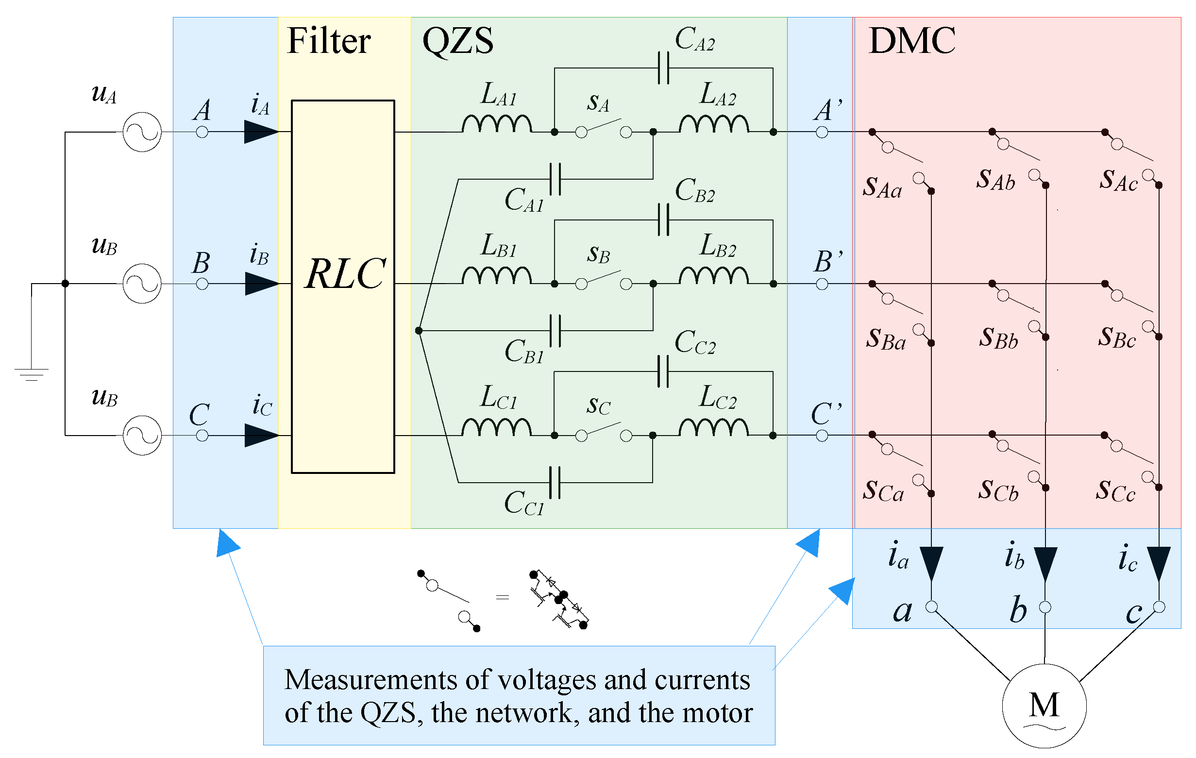
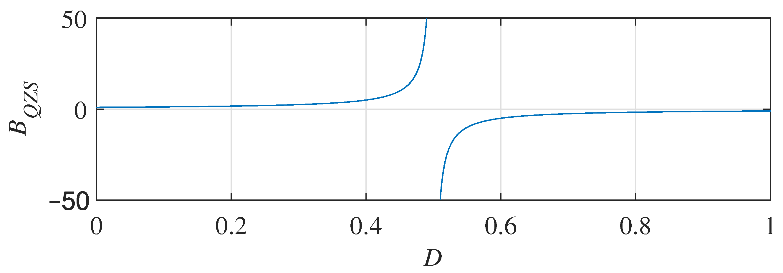
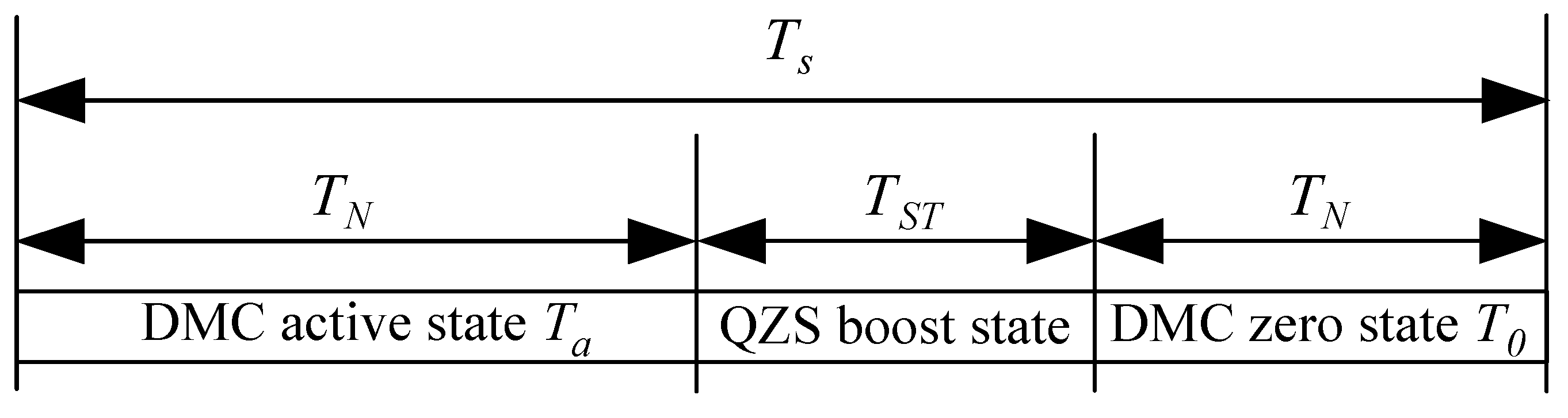
3. Quasi-Z-Source Direct Matrix Converter

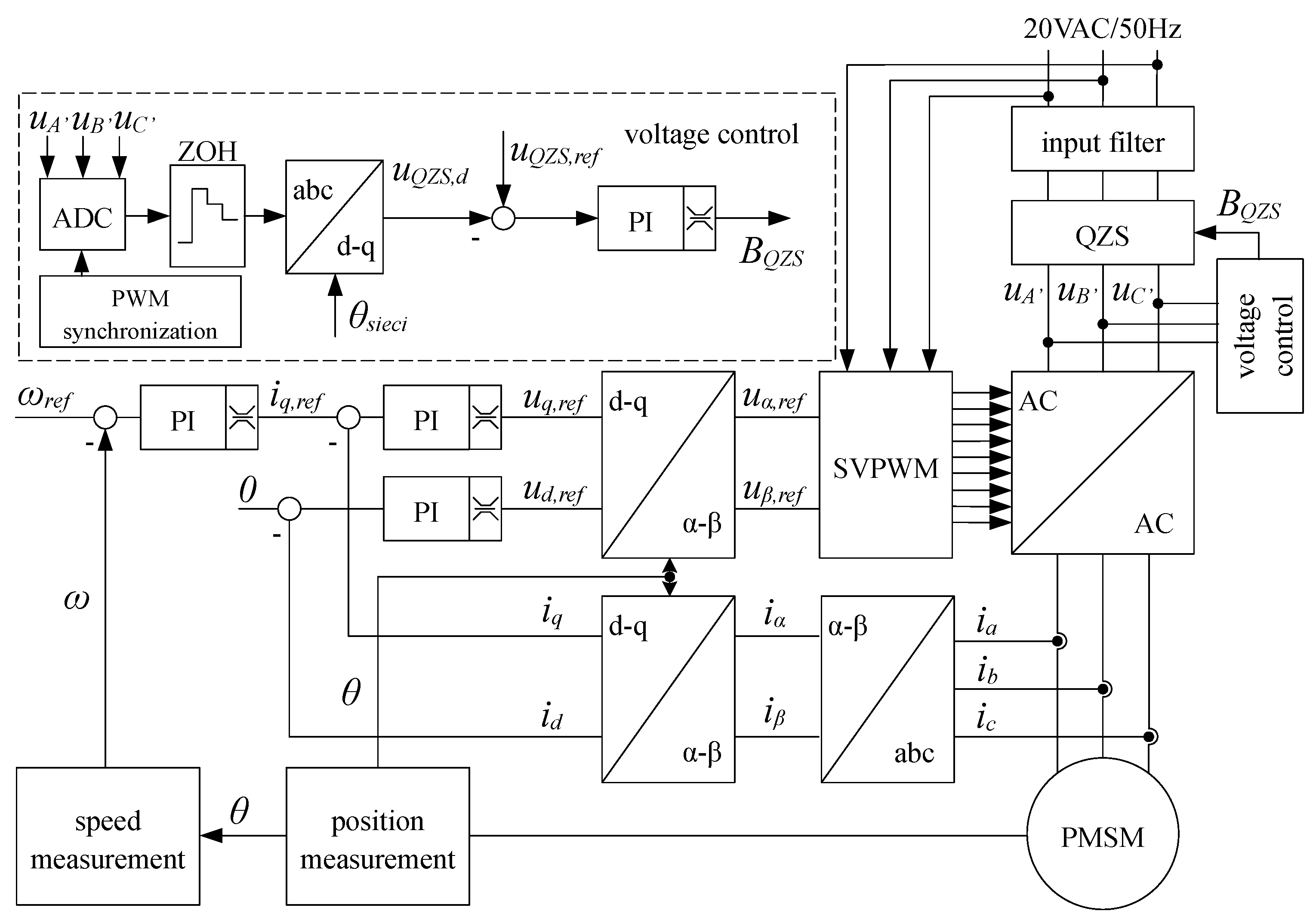
The quasi-Z-source direct matrix converter (QZSDMC) is a type of AC/AC buck-boost converter that allows for both increasing and decreasing the average voltage within one PWM period. QZSDMC utilizes the unchanged topology of the Direct Matrix Converter (DMC), to which a Quasi-Z-Source (QZS) circuit is connected without any additional modifications. The QZS circuit is a boost-type converter that supplies voltage equal to or higher than the grid voltage to the DMC converter, which operates as a buck converter controlling the average voltage from 0 to 0.866 times the voltage at the output of the QZS.

The QZSDMC converter with a grid filter is shown in Figure 1. Three main components of the converter can be identified: the grid filter, the QZS, and the DMC. The grid filter reduces the ripple in the current drawn from the grid by the converter and facilitates the measurement of the voltage between the QZS and DMC. The QZS module is responsible for boosting the input voltage, while the DMC module shapes the average output voltage according to the control system requirements. A detailed description of DMC control can be found in [39,40,41,42,43,44,45]. The device consists of a low-pass RLC filter, which can be constructed in various ways, six inductors ($L_{A1}$, $L_{B1}$, $L_{C1}$, $L_{A2}$, $L_{B2}$, $L_{C2}$), six capacitors ($C_{A1}$, $C_{B1}$, $C_{C1}$, $C_{A2}$, $C_{B2}$, $C_{C2}$), and three power electronic switches in the QZS section and nine switches in the DMC section. Inductors $L_{A1}$, $L_{B1}$, and $L_{C1}$ act as current buffers, preventing step changes in the current drawn from the grid, thus protecting the grid from significant distortions caused by the discontinuous current draw of the device. Inductors $L_{A2}$, $L_{B2}$, and $L_{C2}$ function as current sources, supplying the QZS capacitors with high voltage. Voltage-boosting in the converter is made possible by the use of three additional power electronic switches ($S_A$, $S_B$, $S_C$). These switches are used to control the voltage gain factor of the QZS and should operate synchronously, meaning they can be controlled by a single control signal. In [46], it is proven that, due to the symmetry of the converter, the described passive components should have identical inductance and capacitance values.

The QZSDMC switches between two states during operation [9,47,48]. In the first state, called the Nonshoot-through (NST) state, the switches $S_{ABC}$ are in saturation, allowing the DMC converter to generate the desired output voltage. In the second state, called the shoot-through (ST) state, the switches $S_{ABC}$ are in the off state (blocking), while the switches $S_{Aa}$, $S_{Ba}$, and $S_{Ca}$ are in saturation, creating a short circuit at the output of the QZS. During this state, electrical energy from the source does not reach the DMC and the voltage at the QZS output increases. The diagram illustrating these states of the converter is shown in Figure 2.

For a single switching period $T_s$, the duration of the ST state can be denoted as $T_{ST}$ and the duration of the NST state as $T_N$, such that $T_s=T_{ST}+T_N$. The duty cycle of the ST state is given by: $D={\displaystyle \frac{T_{ST}}{T_s}}$. This duty cycle D represents the fraction of the period during which the converter operates in the shoot-through (ST) state.

Based on Figure 2b, the voltage equations for the ST state can be expressed as [9]:

$$\left[\begin{array}{c}{u}_{AB}\\ u_{BC}\\ u_{CA}\end{array}\right]=\left[\begin{array}{c}{u}_{L_{A1}}\\ u_{L_{B1}}\\ u_{L_{C1}}\end{array}\right]+\left[\begin{array}{c}{u}_{C_{A2}}\\ u_{C_{B2}}\\ u_{C_{C2}}\end{array}\right]-\left[\begin{array}{c}{u}_{C_{B2}}\\ u_{C_{C2}}\\ u_{C_{A2}}\end{array}\right]-\left[\begin{array}{c}{u}_{L_{B1}}\\ u_{L_{C1}}\\ u_{L_{A1}}\end{array}\right]$$

(10)

where: $u_{AB}$, $u_{BC}$, $u_{CA}$—input line-to-line voltages, $u_{Ln}$—voltage drop across the inductor 1 in phase n, $u_{Cn}$—voltage drop across the capacitor 2 in phase n. Based on Figure 2a, the voltage equations for the NST state can also be derived, which can be written as [9]:

$$\left[\begin{array}{c}{u}_{AB}\\ u_{BC}\\ u_{CA}\end{array}\right]=\left[\begin{array}{c}{u}_{L_{A1}}\\ u_{L_{B1}}\\ u_{L_{C1}}\end{array}\right]+\left[\begin{array}{c}{u}_{C_{A2}}\\ u_{C_{B2}}\\ u_{C_{C2}}\end{array}\right]+\left[\begin{array}{c}{u}_{A^{\prime }{B}^{\prime }}\\ u_{B^{\prime }{C}^{\prime }}\\ u_{C^{\prime }{A}^{\prime }}\end{array}\right]-\left[\begin{array}{c}{u}_{C_{B2}}\\ u_{C_{C2}}\\ u_{C_{A2}}\end{array}\right]-\left[\begin{array}{c}{u}_{L_{B1}}\\ u_{L_{C1}}\\ u_{L_{A1}}\end{array}\right]$$

(11)

In the steady state, the average voltage across the inductors over a single operating period of the converter should equal zero. By utilizing the symmetrical capacitor voltages in the three phases, as per [4], we obtain:

$$\left[\begin{array}{c}{u}_{AB}\\ u_{BC}\\ u_{CA}\end{array}\right]={\displaystyle \frac{1}{1-2D}}\left[\begin{array}{c}{u}_{L_{B1}}\\ u_{L_{C1}}\\ u_{L_{A1}}\end{array}\right]$$

(12)

In [4], the boost factor for the QZS is defined as:

$$B_{QZS}={\displaystyle \frac{u_o}{u_i}}={\displaystyle \frac{1}{1-2D}}$$

(13)

where: $u_i$—the amplitude of the input voltage of the QZS, $u_o$—the amplitude of the output voltage of the QZS.

Figure 3 shows the QZSDMC gain as a function of the D duty cycle of the ST state. An asymptotically infinite increase in the gain $B_{QZS}$ can be observed at $D=0.5$. This indicates that, at least theoretically, QZSDMC can achieve arbitrarily high output voltage values. In practice, however, parasitic parameters of the utilized components prevent achieving infinite gains [49].

In this study, the Simple Boost (SB) algorithm was chosen to control the voltage boost [1]. SB control involves adding the ST state during the duration of the zero vector $T_0$ when the load is disconnected from the grid, thereby reducing the impact of voltage-boosting on the load operation. In this method, the duration of the NST state must be at least equal to the duration of the active state $T_a$ in the DMC. This limitation protects the load from errors in controlling the output voltage of the converter. Figure 4 illustrates the sequence of voltage states during a single operating cycle of the QZSDMC.

4. Control System

This research focuses on the issue of controlling the voltage boost of a QZSDMC converter with a grid filter operating in the speed control system of a PMSM. The developed system should enable fast and stable control of the QZS output voltage. Fast control refers to achieving control within a time frame close to the electrical time constants of voltage rise in the QZS converter. Stable control means regulating the QZS output voltage in a way that does not negatively impact the operation of the PMSM speed control system.

The research was conducted on a system whose block diagram is shown in Figure 5. This diagram is divided into two parts: one related to the control of the PMSM torque and the other to the control of the QZS converter output voltage.

The torque control system utilizes vector control, which involves transforming the coordinate system of the machine’s voltages and currents from the $ABC$ frame, associated with the stator, to the $dq$ frame, associated with the rotor of the motor. The mathematical operator used in this process is the Clarke and Park transformation, described by Equation (1). Vector control enables the application of linear single-input, single-output controllers to regulate the motor currents. In this study, PI controllers with saturation and anti-windup mechanisms were used for both current and speed control. A constant power angle control strategy was implemented, where the $i_d$ current controller maintains a fixed reference value of $i_{d_{ref}}=0$ A. This approach ensures a linear relationship between the electromagnetic torque and the $i_q$ current.

In the block diagram presented in Figure 5, the method for controlling the output voltage of the QZS is illustrated. The primary challenge lies in accurately measuring this voltage. Typically, measurements are taken directly across the QZS capacitors. However, in this study, the measurement is performed between the QZS and the DMC, which, while reducing the need for additional measurement devices, introduces challenges related to synchronizing the measurement moments with the PWM signal. Once the voltage value is obtained for a given period, it is maintained using a zero-order hold and then transformed via the Clarke and Park transformation into the $dq$ coordinate system associated with the grid phase angle. This approach converts the three-phase voltage state variables $u_{A^{\prime }}$, $u_{B^{\prime }}$, and $u_{C^{\prime }}$ into a single state variable $u_{QZS}$, corresponding to the d-axis component of the resulting vector. This enables the use of a single linear PI controller to regulate the voltage effectively.

The studies utilized a grid filter whose structure was adapted from [50]. The implementation of this filter reduces the negative impact of the converter’s boost on the grid current, thereby improving the quality of the $u_{QZS}$ voltage measurement in the system. The schematic diagram of the filter is shown in Figure 6. The passive parameters were selected based on Formulas (14)–(16):

$$L_f={\displaystyle \frac{k_F^2}{2{\pi }^2{f}_0^2{C}_F}}$$

(14)

$$R_{ft}=\sqrt{{\displaystyle \frac{L_f}{C_f}}}$$

(15)

$$C_{ft}=4C_f$$

(16)

where $C_F$ is the filter capacitance value, arbitrarily chosen to minimize size, power losses, and current distortion, $k_F$ is the factor determining the offset of the cutoff frequency from the converter’s operating frequency, and $f_0$ is the filter’s cutoff frequency.

The measurement of $u_{QZS}$ is complicated by the pulsed nature of power electronic converters. It is conducted at the $u_{A^{\prime }{B}^{\prime }{C}^{\prime }}$ point (between QZS and DMC), where the zero vectors do not reduce the electrical potential of the lines to zero. A decision must be made on whether the algorithm should measure the voltage during the active vectors or the zero vectors. It was determined that the measurement would be performed during the vector with the greater duty cycle calculated for the given control period.

Figure 7 presents graphs related to the measurement of the $u_{QZS}$ voltage. The first part of the figure shows the value of the counter synchronizing the triggering of the QZSDMC control algorithm over time, denoted here as t. This counter operates with a period of $T_{PWM}$. Zero vector $T_0$ is marked with arrows. The second part of the figure zooms in on a single phase of the $u_{A^{\prime }{B}^{\prime }{C}^{\prime }}$ voltage. The blue line indicates the $u_{A^{\prime }}$ voltage behind the QZS converter, while the purple line represents the measured voltage used in the $u_{QZS}$ voltage controller. It highlights the measurement moment $T_m$, located at the midpoint of the zero vector. The $T_m$ period is equal to the control period $T_s$. The measurement occurs at the moment:

$$tmod{T}_{\mathrm{PWM}}={\displaystyle \frac{T_{\mathrm{PWM}}(d_{ST}+1)}{2}}$$

(17)

The third graph shows all three phases of the $u_{A^{\prime }{B}^{\prime }{C}^{\prime }}$ voltage, along with the resulting measurements and the highlighted $ST$ state, where the voltage between the QZS and DMC is zero (phases are short-circuited). The last graph displays the voltage on the motor phases, with the active vector period $T_a$ marked.

Figure 7 shows the measurement of $u_{QZS}$ at a magnification that allows focusing on individual PWM periods. This view helps in understanding the detailed operation of the process but does not represent the measurements used for voltage control. These measurements are depicted in Figure 8. The observation range here is 40 ms, covering the duration of two steps in the boost factor $B_{QZS}$. In the first part of the figure, the three-phase voltage $u_{A^{\prime }{B}^{\prime }{C}^{\prime }}$ is shown along with its close-up view. These are raw, unprocessed simulation data, which are challenging to analyze in the control system due to the $ST$ states. The second graph shows the same data after applying the algorithm synchronizing the measurements with the PWM. It can be observed that the resulting signals resemble the envelopes of the signals from the first graph. The third graph presents the data after synchronization and $dq$-transformation. Such a signal can now be effectively used in a linear controller for regulating the voltage $u_{QZS}$.

5. Simulation Research

The simulation studies were conducted using the Matlab 2019a Simulink environment and the Simscape library. Continuous elements, such as the PMSM motor and electronic components, were simulated with a step size of 250 ns. Control elements were calculated with a step size equal to $T_{PWM}=50$$\mathsf{\mu }\mathrm{s}$. The Simscape library facilitates the simulation of electronic components such as resistors, inductors, capacitors, diodes, and transistors. The models used allow for the inclusion of parasitic parameters, enhancing modeling accuracy. In the presented tests, converters and filters were built from these components. Due to additional complexity and minimal impact on the final results, bidirectional power electronic switches were approximated using ideal bidirectional switches. The simulations employed a ready-made PMSM model available within Matlab Simscape [51], whose parameters were taken from PMSM used in laboratory stand (Teknic M2310P-LN-04K) (

Table 1. Rated parameters of PMSM.

Parameter	Symbol	Value
Maximum voltage	$u_{max}$	40 V
Rated voltage	$u_n$	24 V
Rated current	$i_n$	$7.1$ A
Electromagnetic torque	$k_M$	$0.0122{\displaystyle \frac{\mathrm{N}·\mathrm{m}}{\mathrm{A}}}$
Rated speed	${\omega }_n$	$628{\displaystyle \frac{\mathrm{rad}}{\mathrm{s}}}$
Number of pole pairs	p	3
Stator resistance	$R_s$	$0.72$$\mathrm{\Omega }$
Inductance in the d-axis	$L_d$	336 $\mathsf{\mu }\mathrm{H}$
Inductance in the q-axis	$L_q$	336 $\mathsf{\mu }\mathrm{H}$

). Similarly, a model was used for a step-down transformer reducing the mains voltage (50 Hz frequency, 325 V amplitude, corresponding to an RMS value of 230 V) to a voltage with an amplitude of 20 V. The network filter model was constructed using basic elements, and its schematic diagram is shown in Figure 6.

The parameters of the network filter, along with the QZSDMC converter parameters, are described in

Table 2. Parameters of the RLC network filter.

Parameter	Symbol	Value
Filter inductance	$L_f$	375 $\mathsf{\mu }\mathrm{H}$
Filter capacitance	$C_f$	$0.3$ $\mathsf{\mu }\mathrm{F}$
Damping capacitance	$C_{ft}$	$1.2$ $\mathsf{\mu }\mathrm{F}$
Damping resistance	$R_{ft}$	35 $\mathrm{\Omega }$

and

Table 3. Passive parameters of the QZSDMC converter.

Parameter	Symbol	Value
QZS inductance	$L_{ABC}$	30 $\mathsf{\mu }\mathrm{H}$
QZS capacitance	$C_{ABC}$	10 $\mathsf{\mu }\mathrm{F}$

.

During the simulation studies, the effect of voltage surges $u_{QZS}$ in an open-loop system (without $B_{QZS}$ boost regulation) on the voltage across the PMSM and the current drawn from the grid was examined (Figure 9). In the test, the motor shaft rotated at a speed of 200 rad/s, and the current $i_q$ had a value of 2 A. The machine’s moment of inertia was artificially increased to ensure its speed and power remained unchanged. The voltage boost $B_{QZS}$ varied randomly in the range of 1 to 3. In Figure 9, it can be observed that the current drawn from the grid correlates with the voltage boost: the higher the boost, the greater the current. During the studies, it was noted that exciting the system with rectangular voltage boost steps caused significant oscillations. Even a slight limitation of the derivative of the voltage boost signal reduced their occurrence. This limitation was applied in the presented test.

The design of automatic control systems typically begins with gaining knowledge about the controlled object. One of the methods used for system identification is applying a step change to its input. These signals can have different steady-state values and time delays, and they depend on the specific characteristics of the object. In the presented studies, during the simulation, it was observed that exciting the object with step changes of varying amplitudes resulted in different responses at the output. Based on this observation, a step-like reference signal was created. It changed every $0.02$ s in the range from $B_{QZS}=1$ to $B_{QZS}=5$ with a step size of $0.5$. Such excitation allowed testing of how the height of the voltage $u_{QZS}$ influences the time constants and the gains of the object. The response of the QZS to the described signal is shown in Figure 10. It can be seen that the initial oscillatory behavior decreases with increasing voltage while the gain of the object remains unchanged.

Figure 11 shows the voltages $u_{QZS}$ for four selected steps of $B_{QZS}$ with values $\langle 1.5,2.5,4,5\rangle$. As seen, the character of the object’s oscillations changes. As the output voltage decreases, the frequency of oscillations increases, and the damping decreases. Due to the increase in damping, the oscillation frequency could only be determined for the first two steps (a) and (b), which were 1845 Hz and 1152 Hz, respectively. The rise time was $0.15$ ms for response (a), $0.15$ ms for (b), $0.45$ ms for (c), and $0.5$ ms for (d). It can also be observed that non-minimum phase behavior appears in the system. Based on this behavior, it was decided to investigate this characteristic on a real system.

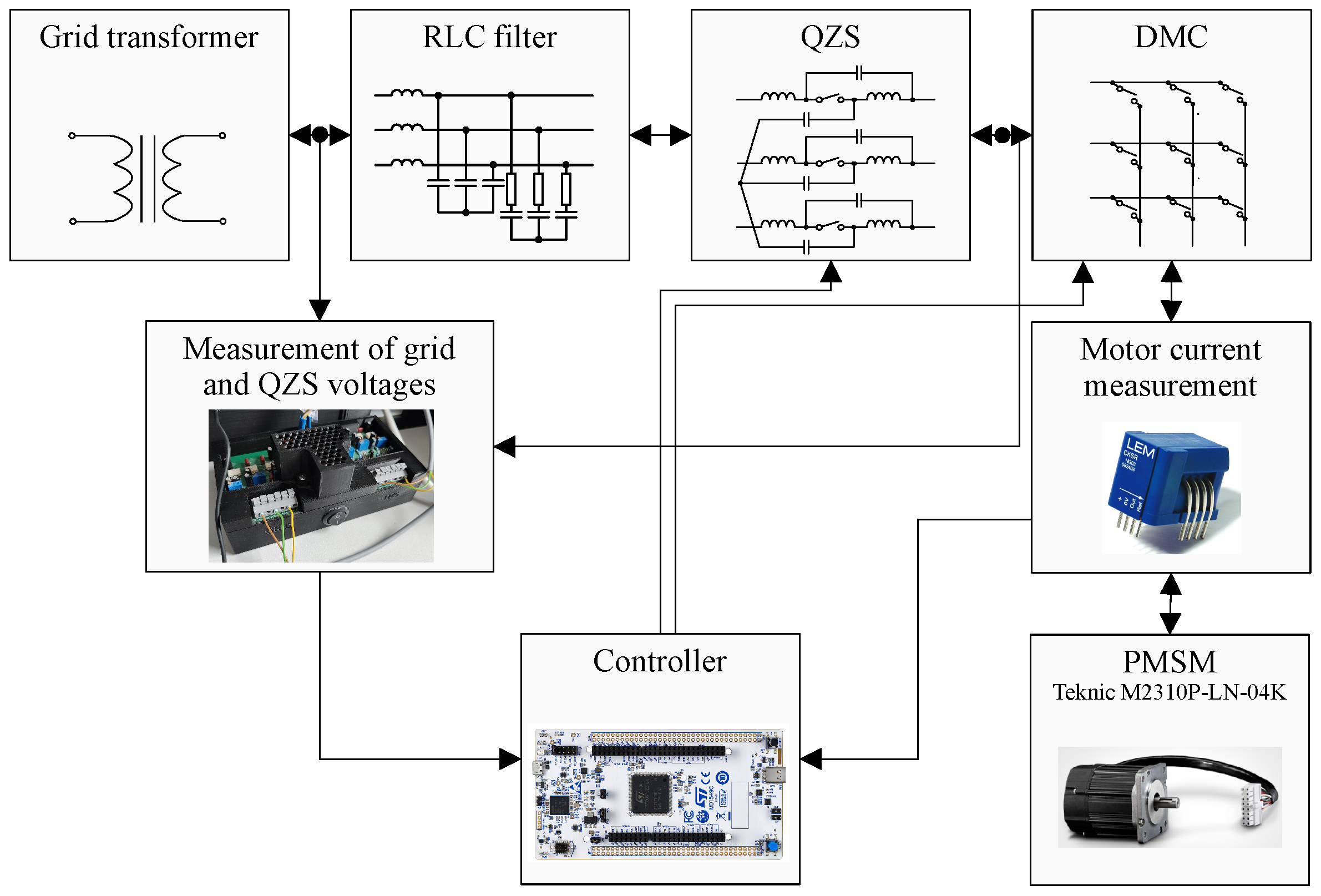
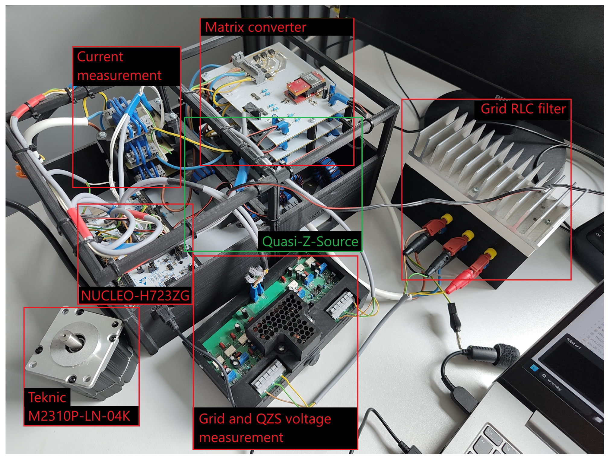
6. Experimental Research

The block diagram of the experimental setup used in the studies is shown in Figure 12. Each module of the device, represented as a single block in the diagram, is connected to the other modules via electrical connectors, which allow for the disconnection of a particular part. The drive system was designed in a modular way, which facilitates easy replacement of components or their reorganization. The experimental setup prepared for the studies is shown in Figure 13.

The prototype of the PMSM drive powered by a Quasi-Z-Source inverter with a matrix converter, presented in this section, was used for research on voltage boost control in such systems. The literature does not contain publications related to the control of the output voltage from QZSDMC that consider the problem within a time window close to the time constants of the system. The publications on this topic only describe the global effect of changes in the QZS gain on the system, focusing on time scales that span multiple cycles of the network’s sinusoidal wave. This approach does not allow for the study of controllers that provide rapid changes in the controlled voltage. To select the parameters of such a controller, the work must begin with system identification, which, in this case, is especially important due to the demonstration of nonlinearities during the simulation tests.

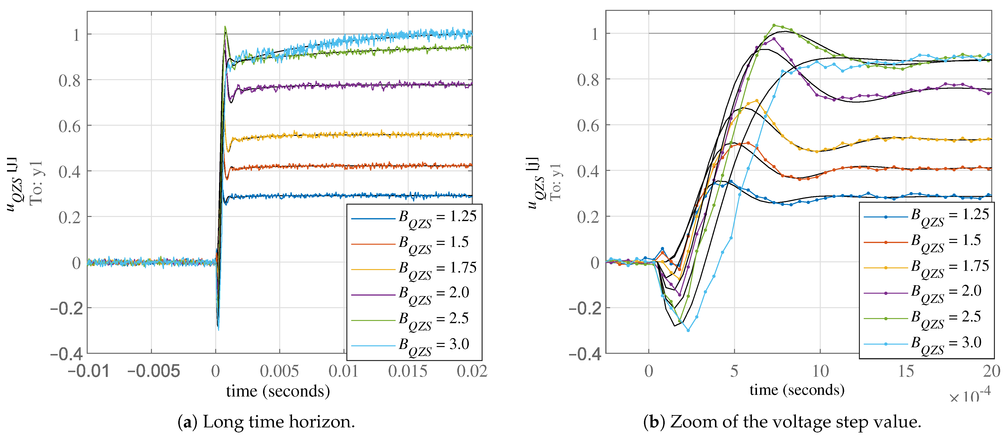
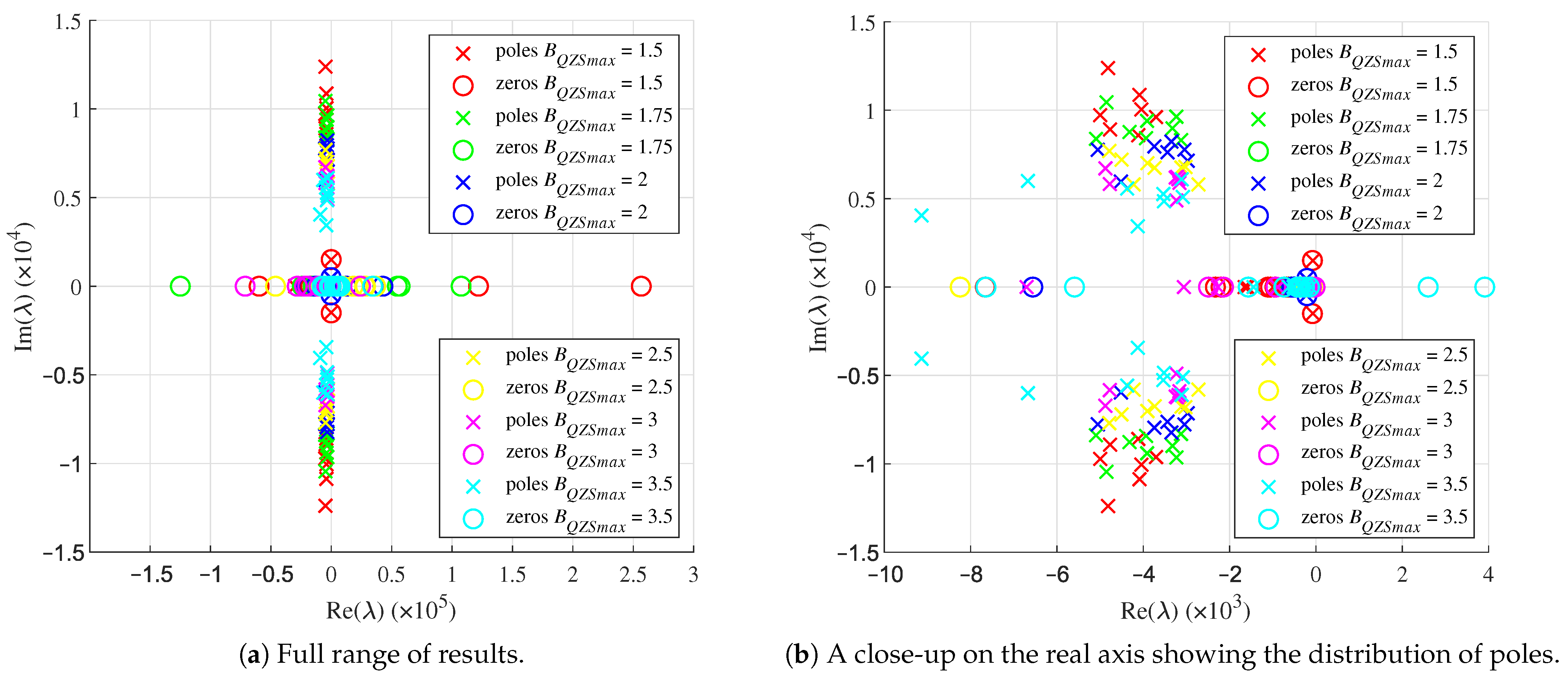
6.1. System Identification

During the simulation tests, potential variability of the system depending on the forced gain in the system was observed. This variability could significantly affect the operation of the system in a closed-loop feedback control. Therefore, identification is crucial to prove its existence and determine its scope. This information allows for the selection of the optimal control strategy that ensures stable system operation. In this work, offline identification methods were chosen due to the risk of damaging the converter with high voltages that can occur in the case of incorrect QZS control.

To eliminate noise and obtain high-quality datasets for identification, all measurements were performed in a series of 20 identical tests. Each set of measurements was subjected to a filtering process to remove disturbances. The filtering procedure involved calculating the arithmetic mean of the measurements taken at the same time point across all test series. This process can be described by the following formula:

$${\overline{u}}_{QZS}\left(k\right)=\sum _{j=1}^n{\displaystyle \frac{u_{QZS}(k,j)}{n}}$$

(18)

where ${\overline{u}}_{QZS}$ is the filtered measurement of the voltage at the QZS, $u_{QZS}$ is the voltage measurement at the QZS with index j, k is the sample number of the measurement signal, and n is the maximum number of collected datasets.

This approach preserved the information about the object’s characteristics while removing randomly occurring disturbances.

During the simulation tests, it was observed that the gain $B_{QZS}$ affects the character of the response of the simulated system. Therefore, it was decided to check how changes in this parameter influence the behavior of the real object. Eight different values of the maximum gain were chosen for testing, as presented below:

$$B_{QZ{S}_{max}}=\langle 1.25;1.5;1.75;2.0;2.5;3.0;3.5\rangle$$

(19)

These values determined the maximum voltage $u_{QZS}$ for the generated step responses. These steps gradually decreased their amplitude over time by increasing the minimum voltage of each step, creating a staircase-like characteristic. The minimum value of the voltage step is expressed by Equation (20).

$$B_{QZ{S}_{min}}=\left\{\begin{array}{c}1,\hfill \\ B_{QZ{S}_{max}}-0.8·(B_{QZ{S}_{max}}-1),\hfill \\ B_{QZ{S}_{max}}-0.7·(B_{QZ{S}_{max}}-1),\hfill \\ B_{QZ{S}_{max}}-0.6·(B_{QZ{S}_{max}}-1),\hfill \\ B_{QZ{S}_{max}}-0.5·(B_{QZ{S}_{max}}-1),\hfill \\ B_{QZ{S}_{max}}-0.4·(B_{QZ{S}_{max}}-1),\hfill \\ B_{QZ{S}_{max}}-0.3·(B_{QZ{S}_{max}}-1),\hfill \\ B_{QZ{S}_{max}}-0.2·(B_{QZ{S}_{max}}-1),\hfill \end{array}\right.$$

(20)

This choice of identification signals allows for testing a wide range of excitations, both absolute and relative voltage amplitudes, while also reducing the number of tests required.

The research used the Ident tool in the Matlab environment, which provides a convenient method for identifying dynamic systems based on experimental data. It allows for modeling transfer functions, state-space equations, and other mathematical models that best reflect the system’s behavior based on the collected data. Due to the ease of analysis, transfer function models were used to model the studied object.

The Ident tool requires the user to select the order of the transfer function in the prepared model. This order must be high enough to correctly capture the dynamics of the object, but too high an order increases computational complexity and makes the analysis more difficult. For this reason, the transfer function order should be chosen as low as possible while maintaining satisfactory accuracy. In these studies, it was decided that the model should have at least 90% fit to experimental data, which, considering the above considerations, allowed selecting two zeros and three poles for the transfer function.

In the presented studies, identification was performed using a nonlinear least squares method with an automatically selected direction search method.

The creator of the tool, in its documentation [52], recommends properly preparing experimental data to maximize the linear model’s fit to the physical object. According to the provided documentation, short time horizons before and after the unit step (10 ms before the step and 20 ms after the step) were selected. The signals were normalized in amplitude relative to the maximum value of the voltage $u_{QZS}$ obtained at the highest tested gain $B_{QZS}=3.5$. Additionally, the signal’s average value, calculated when the converter was not performing voltage-boosting, was subtracted from the signal. The data preparation can be described by the following equation:

$${\overline{u}}_{QZSnorm}={\displaystyle \frac{{\overline{u}}_{QZS}-\frac{1}{b}{\sum }_{k=1}^b{\overline{u}}_{QZ{S}_{B_{QZS}=1}}\left(k\right)}{\frac{1}{b}{\sum }_{k=1}^b{\overline{u}}_{QZ{S}_{B_{QZS}=3,5}}\left(k\right)-\frac{1}{b}{\sum }_{k=1}^b{\overline{u}}_{QZ{S}_{B_{QZS}=1}}\left(k\right)}}$$

(21)

where ${\overline{u}}_{QZSnorm}$ is the normalized voltage signal ready for identification, ${\overline{u}}_{QZ{S}_{B_{QZS}=x}}$ is the averaged voltage measurement at gain x, calculated using Formula (18), k is the sample number of the measurement vector, and b is the number of the last sample of the measurement vector before the change in voltage gain.

In this study, a transfer function model was created for each of the obtained step responses—8 maximum gain values $B_{QZ{S}_{max}}$, with each having 8 values of $B_{QZ{S}_{min}}$, which together created 64 models. However, it should be noted that the voltage boost $B_{QZ{S}_{max}}=1.1$ did not provide valid solutions for the Ident algorithm, meaning that 56 different transfer function models were realistically created. Several of these models, created for $B_{QZ{S}_{min}}=1$, are presented in

Table 4. Obtained system transfer functions for $B_{QZ{S}_{max}}=\langle 1.25;1.5;1.75;2.0;2.5;3.0;3.5\rangle$ and $B_{QZ{S}_{min}}=1$.

${\mathit{B}}_{{\mathbf{QZS}}_{\mathbf{max}}}$	System Transfer Function
1.25	model order too low
1.5	${\displaystyle \frac{-629.6s^2+1.612·{10}^{8}s+1.033·{10}^{11}}{s^3+8694s^2+1.222·{10}^{8}s+7.077·{10}^{10}}}$
1.75	${\displaystyle \frac{-969s^2+1.037·{10}^{8}s+5.249·{10}^{10}}{s^3+6727s^2+8.177·{10}^{7}s+3.729·{10}^{10}}}$
2	${\displaystyle \frac{-6177s^2+7.325·{10}^{7}s+3.988·{10}^{10}}{s^3+6423s^2+6.268·{10}^{7}s+2.855·{10}^{10}}}$
2.5	${\displaystyle \frac{-5659s^2+4.753·{10}^{7}s+2.057·{10}^{10}}{s^3+5833s^2+4.316·{10}^{7}s+1.588·{10}^{10}}}$
3	${\displaystyle \frac{-5789s^2+3.688·{10}^{7}s+4.036·{10}^9}{s^3+6570s^2+3.507·{10}^{7}s+3.388·{10}^9}}$
3.5	${\displaystyle \frac{-5752s^2+2.384·{10}^{7}s+3.696·{10}^9}{s^3+8383s^2+2.989·{10}^{7}s+3.641·{10}^9}}$

. Unlike $B_{QZ{S}_{max}}=1.1$, the voltage boost $B_{QZ{S}_{max}}=1.25$ provided valid identification results, but the order of the chosen model was too low. Increasing the model order led to the creation of a correct transfer function. However, it was decided that comparing a model with a higher order than the others would not allow for meaningful conclusions from this study.

Analyzing the obtained data, part of which is presented in Table 4, it can be observed that the transfer functions found during identification differ from each other in terms of their parameters. The coefficients of the numerator and denominator associated with the s-operators of low powers $\langle 0;1\rangle$ show a clear downward trend, starting from the lowest voltage boost to the highest one. This indicates that the models exhibit some variation. The existence of this trend suggests that the variation is not merely a measurement error caused by noise but rather that the object demonstrates some variability in its parameters dependent on the voltage boost.

In Figure 14, the response of six selected transfer function models, presented in Table 4, to a normalized $B_{QZS}$ step change is shown. The figure overlays the data used in Ident with the results obtained from the simulation of the model. Figure 14a shows the response over a long time horizon. This figure demonstrates the convergence of all the models, including the one for $B_{QZ{S}_{max}}=3.5$, where the system, after an initial step, continues to slowly increase the output value. The voltage step rise times are not easily analyzed in Figure 14a, which is why Figure 14b is presented with a time scale reduced by a factor of ten for better clarity. In Figure 14b, it can be seen that the models correctly capture the system’s behavior, including oscillations and non-minimum phase characteristics. Attention can also be drawn to the time constants that characterize the object. Depending on the signal amplitude, the system reaches a steady state within 1.5 ms, and the rise times of the responses are on the order of hundreds of microseconds, placing high computational demands on the controller. The results for the remaining step responses were checked in the same manner, but due to the clutter in the figure containing all the models, only selected results are shown. This test confirms the accurate identification of the transfer function models for the system in 56 operating points.

One of the methods for studying the variability of the transfer function is to check the distribution of its zeros and poles on a complex plane plot. This method allows for a graphical representation of the system’s frequency characteristics, which helps to understand its behavior under different operating conditions. It enables a quick assessment of the system’s stability and its response to changes in parameters. This type of analysis is shown in Figure 15. The plot consists of two elements. Figure 15a presents the full range of the real axis, which allows for the analysis of the distribution of the zeros of the transfer function models. From the figure, it can be seen that the zeros vary significantly depending on the chosen gain. Figure 15b presents a zoomed-in view of the real axis, enabling a detailed analysis of the distribution of the system’s poles. The plot shows that no pole has a positive real value, indicating that the system is stable within the investigated range. The poles also frequently occur in pairs symmetrically around the real axis, which suggests that the system is oscillatory. In Figure 15, poles and zeros for a given gain $B_{QZ{S}_{max}}$ are marked in the same color, allowing for the analysis of poles depending on this parameter. An obvious conclusion is the change in the region where the system’s poles occur. As $B_{QZ{S}_{max}}$ increases, the poles have a higher average absolute value of the imaginary part (they move away from the real axis). The displacement from the complex axis, and thus the real part of the poles, shows no significant changes. This observation can be crucial when selecting a QZS voltage controller. It may be possible to choose its parameters based on the average of all poles or, as seems reasonable, apply a tunable controller with gain values recorded in the table, which depend on the value of the voltage gain $B_{QZ{S}_{max}}$.

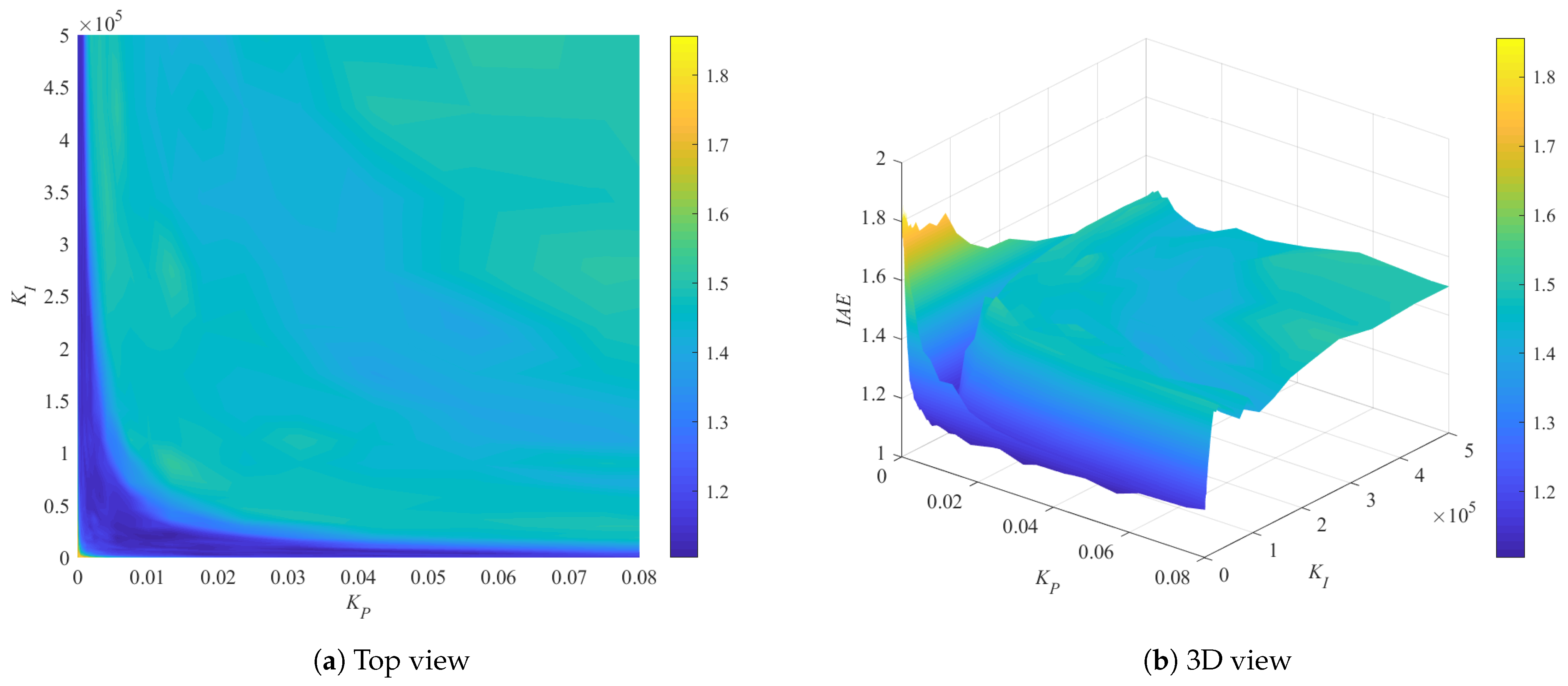
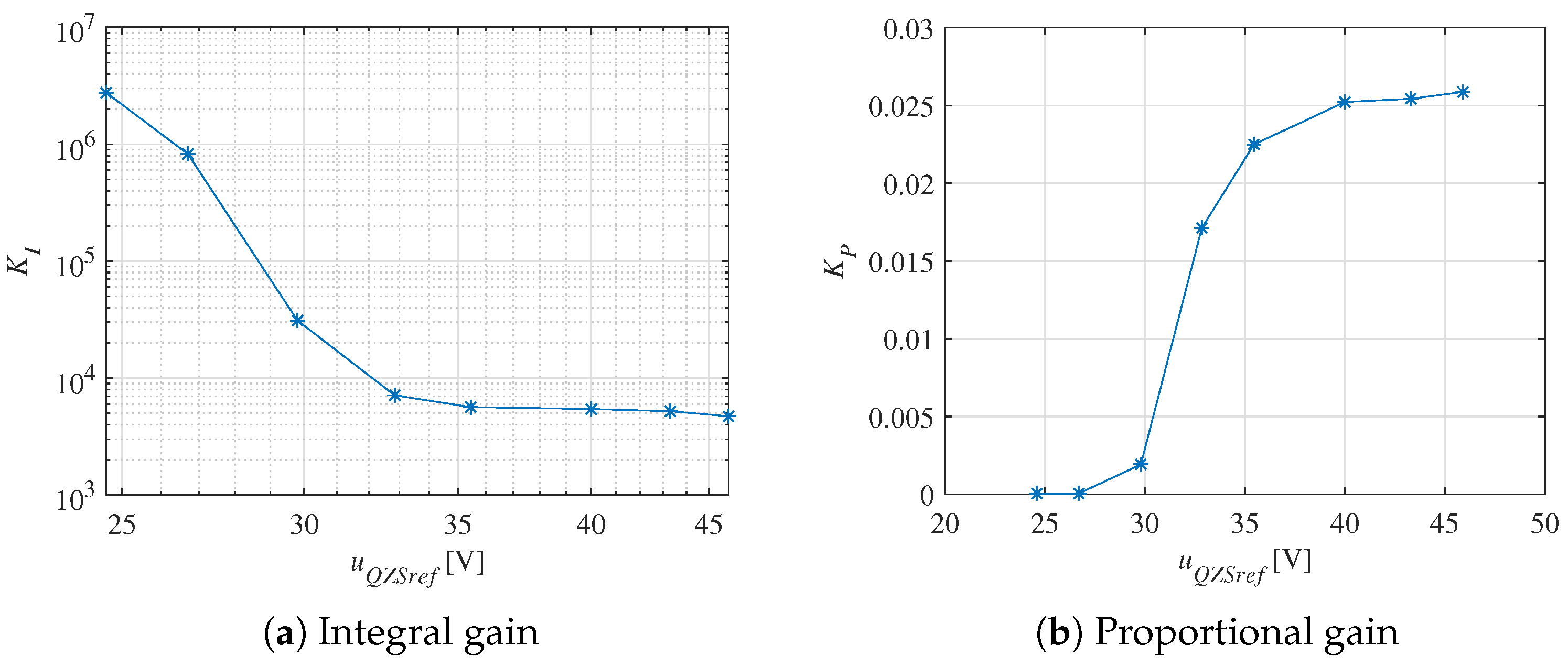
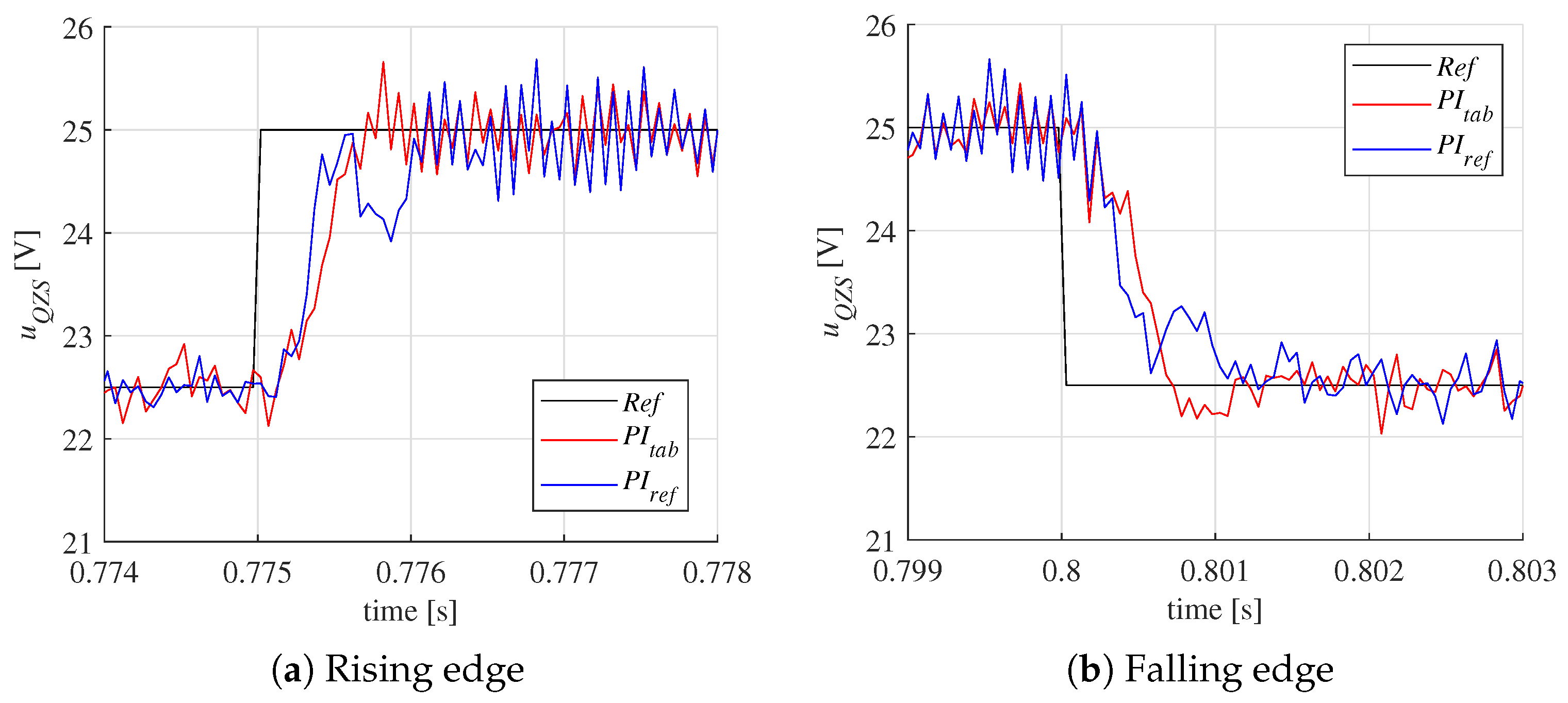
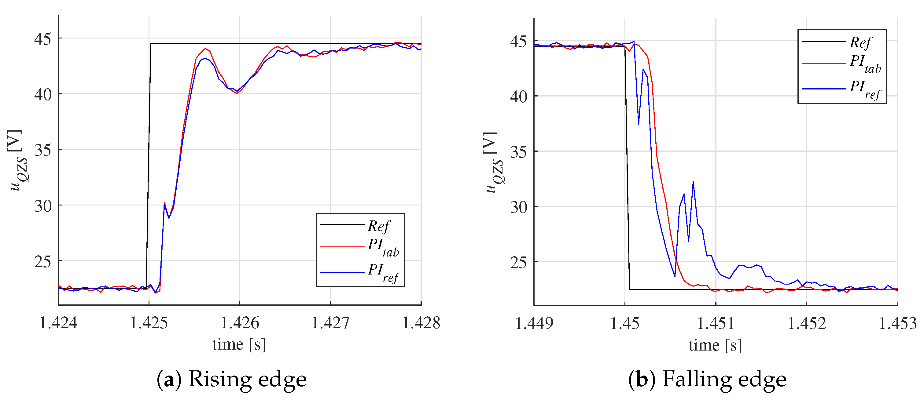
6.2. Controller Design

Linear controllers, including the proportional-integral (PI) controller and the proportional- integral-derivative (PID) controller, are among the most commonly used controllers in the field of automation. They find application in a wide range of systems, from simple temperature control loops to advanced motor control systems.

In this work, linear controllers with constraints and an anti-windup mechanism were used as a key element of the control strategy. This decision stems from the need to ensure not only efficiency but also safety in the context of controlling the voltage supplied to the PMSM motor. To achieve this, a PI controller was applied, which utilizes voltage measurements on the converter, enabling proper voltage regulation.

One of the advantages of this approach is the assurance of maintaining the voltage at the PMSM terminals within safe limits, ensuring not only optimal operating conditions for the drive but also minimizing the risk of undesirable phenomena such as overload or overheating.

Tunable PI controllers with gain values stored in a table format are a variant of traditional PI controllers that use predefined lookup tables to determine the controller parameters based on specific input conditions [53,54,55]. These tables typically map input parameters, such as error and its derivative, to corresponding controller parameters, such as proportional and integral gains. This approach offers advantages in systems where real-time calculation of new parameters is impractical due to limited computational power or where precise tuning is required for different operating conditions.

However, it is important to ensure that the lookup table adequately covers the range of operating conditions and that the stored values accurately reflect the system’s response to various inputs.

The existence of a correlation between the average pole positions on the complex plane and the gain $B_{QZS}$ allows for the use of controllers with gain values stored in a lookup table format. This approach improves the solution’s robustness and regulation quality without increasing the computational overhead while ensuring the system’s determinism.

The dependence of the controller parameters on the current reference signal $u_{QZ{S}_{ref}}$ is tied to the regulation object’s behavior. Its response mainly depends on the voltage (gain) at which a particular step ends. This can be inferred from the appearance of non-minimum phase behavior in the object’s response, as shown in Figure 14. The figure depicts steps starting at the same voltage but ending at different maximum voltage values. Non-minimum phase behavior occurs before the voltage reaches the steady-state value. In such cases, it seems reasonable to set the reference value as a parameter that switches the operating points of the controller.

The number of different values for the PI controller’s gain, or the number of its operating points, must strike a balance between the time spent searching for parameter values and the quality of regulation. In this study, it was decided that parameter selection would be based on voltages resulting from the application of voltage boosts described by Equation (19). The resulting voltage values were:

$${\mathbf{U}}_{QZ{S}_{ref}}=\left[\begin{array}{cccccccc}24.6& 26.7& 29.8& 32.85& 35.45& 40& 43.3& 45.9\end{array}\right]$$

(22)

In this study, it was decided that the best method to check whether the voltage regulation of the QZSDMC converter, performed at different operating points, yields better results than a single, fixed controller is the optimal selection of PI controller parameters involved in the experiment. The optimization process can ensure the best possible solution in terms of minimizing the cost function. This means that if the controllers are correctly chosen using the optimization method, it would be difficult or even impossible to select controllers that achieve smaller values of the quality index. Therefore, if a controller that adjusts its gains using a lookup table achieves better performance than a controller optimized for the middle reference voltage $u_{QZ{S}_{ref}}$, it could confirm that regulation at multiple operating points of the system is better than using a single, unchanging controller.

In the presented studies, the Hooke-Jeeves method, a gradient-free optimization algorithm named after its authors, was used to find the optimal values of the PI controller parameters [56,57]. The objective function used in the optimization was expressed by the formula:

$$IAE={\int }_0^t\left|u_{QZ{S}_{ref}}-u_{QZS}\right|dt$$

(23)

The termination condition of the algorithm was the achievement of a smaller jump amplitude value in each direction than an arbitrarily selected tolerance parameter. This parameter was chosen experimentally to ensure the algorithm achieved the best possible accuracy in finding the parameters and maintained convergence within a finite time. In practice, the optimizer found about 2000 points with a lower cost function value than the previous point for each linearization point. This resulted in tens of thousands of experiments to find the controller parameters at a single operating point. The algorithm was modified so that each increase in the jump amplitude was twice as large as its decrease. As a result, the algorithm significantly increased the search time for the optimum, but the possibility of getting stuck in a local optimum was considerably reduced.

In order to visualize the results of the optimization algorithm, it was decided to present the values of the objective function found for a single operating point and given parameters $K_P$ and $K_I$ in the form of a three-dimensional surface (Figure 16). A clear trend is visible here, where the objective function decreases within the hyperbolic region near the coordinate axes. The resulting grid of points was used to determine the optimization boundaries, which during the initial tests were set as $(K_{P_{max}}<1)\wedge (K_{P_{min}}>0)$ and $(K_{I_{max}}<5,000,000)\wedge (K_{I_{min}}>1)$. Subsequently, during further tests, the maximum proportional gain was reduced to $(K_{P_{max}}<0.05)$ due to the solutions that tended towards values smaller than $K_{P_{max}}=1$.

The optimization was performed while the system operated with a deterministic excitation vector $u_{QZ{S}_{ref}}$. The excitations began from the supply voltage value, and then the maximum jump value increased by 1.5 V with each subsequent jump. During the optimization, the regulator could freely switch its gains $K_P$ and $K_I$ to the gains ${\mathbf{K}}_{\mathbf{P}}$ and ${\mathbf{K}}_{\mathbf{I}}$ stored in the table. Switching occurred when the reference voltage $u_{QZ{S}_{ref}}$ was closer to another voltage point stored in the table ${\mathbf{U}}_{QZ{S}_{ref}}$. However, it should be noted that at any given time, optimization was applied only to a single row of the ${\mathbf{K}}_{\mathbf{P}}$ and ${\mathbf{K}}_{\mathbf{I}}$ gain table. This ensured the natural operation of the regulator while simultaneously optimizing its single operating point. The range of voltages describing the switching of the regulator’s gains was expressed using Formula (26).

$$K_P={\mathbf{K}}_{\mathbf{P}}\left[i\right]$$

(24)

$$K_I={\mathbf{K}}_{\mathbf{I}}\left[i\right]$$

(25)

$$\begin{array}{c}\hfill i=\underset{k}{\mathrm{argmin}}\left(\left|u_{QZ{S}_{ref}}-{\mathbf{U}}_{QZ{S}_{ref}}\left[k\right]\right|\right),k=0,1,2,\dots ,7\end{array}$$

(26)

The optimization algorithm described above found solutions for the eight planned sets of voltage regulator PI gains $u_{QZS}$ in the experiment. These gains were stored in

Table 5. Optimized $u_{QZS}$ controller gains.

${\mathit{K}}_{\mathit{I}}$	${\mathit{K}}_{\mathit{P}}$	${\mathit{u}}_{{\mathbf{QZS}}_{\mathbf{ref}}}$[V]
$2,760,000$	$0.0000559$	$24.6$
$825,000$	$0.000056$	$26.7$
$31,000$	$0.00193$	$29.8$
7120	$0.0171$	$32.85$
5640	$0.0225$	$35.45$
5430	$0.0252$	40
5210	$0.0254$	$43.3$
4710	$0.0259$	$45.9$

. In the presented results, a certain trend can be observed: the higher the reference voltage, the smaller the $K_I$ and the larger the $K_P$. However, these gains depend non-linearly on the switching point. These functions are shown in Figure 17. Figure 17a contains data for $K_I$, which is presented on a logarithmic scale due to the large variability of the parameter. Figure 17b consists of the $K_P$ gains. Their relatively small variability allowed the results to be presented on a linear scale. From both of these plots, it is clearly visible that in Figure 17a, the trend is non-increasing, while in Figure 17b, the trend is non-decreasing.

The quality of the voltage regulator’s performance was evaluated by comparing it to a traditional linear PI controller with fixed parameters, referred to as the reference controller ($P{I}_{ref}$) below. In this work, a controller with variable gains ($P{I}_{tab}$) is compared to a controller with fixed gains, tuned for the middle value of the voltage $u_{QZS}$ through optimization. In practice, this means that the controller with switching gains is compared to a controller with gains from the middle of the table.

The parameters of the controller used are:

$$K_P=0.0225$$

(27)

$$K_I=5640$$

(28)

During the experiments, it was decided that the controllers would be tested using a reference signal $u_{QZ{S}_{ref}}$ containing 16 unit step changes, always starting from the supply voltage. Each subsequent step is greater than the previous one by 1.5 V, so the last step is approximately twice the supply voltage. This signal was applied to the control system with both the reference and tunable controllers. This test allows the evaluation of the controllers at different operating points, which depend on the amplitude and voltage value of the QZS.

During the test, the settling time of the control system response was also measured. It was assumed that the voltage should remain within a $\pm 0.5$ V range. This tolerance was determined as the boundary of the measurement noise occurring in the steady state.

In Figure 18, the following steps are shown: Figure 18a—an increase in voltage by 2.5 V, and Figure 18b—a decrease in voltage by the same amount. It can be observed that the waveforms favor $P{I}_{tab}$. The reference controller has a settling time of 985 $\mathsf{\mu }\mathrm{s}$, while the tunable controller achieves a settling time of 518 $\mathsf{\mu }\mathrm{s}$. The latter reaches the setpoint without introducing additional oscillations, which would otherwise slow down the regulation process and introduce extra disturbances into the PMSM motor current regulation system.

In Figure 19, step changes in the reference voltage with an amplitude of 13 V are shown. The voltage value to which the voltage is increased is chosen so that the reference controller operates under optimal conditions. In this case, both systems being tested have the same parameters. This fact is evident in part (a) of Figure 19. If measurement noise is disregarded, the responses are identical with equal settling time. However, Figure 19b shows the advantage of the tunable controller, which becomes apparent after the $P{I}_{tab}$ controller switches to the values derived from optimization for lower reference voltages. This advantage is the absence of additional oscillations in the response, allowing the system to reach the setpoint more quickly. In this case, the settling time is $1.5$ ms for $P{I}_{ref}$ and 1 ms for $P{I}_{tab}$.

Figure 20 shows a step change in the voltage with an amplitude of 22 V. Similar behavior of both controllers can be observed after the rising edge of $u_{QZ{S}_{ref}}$. The tunable controller exhibits larger oscillation amplitudes, but this does not affect the settling time, which remains the same for both controllers. However, the situation is different for the falling edge, where, despite the same step amplitude, the control systems behave quite differently. After switching the $P{I}_{tab}$ controller to the parameters optimized for lower gains, a clearly shorter settling time and fewer oscillations are observed. In contrast, during the regulation with $P{I}_{ref}$, noticeable oscillations appear in the system’s response, which prolongs the process. The settling time of the control system is 2.1 ms for $P{I}_{ref}$ and 686 $\mathsf{\mu }\mathrm{s}$ for $P{I}_{tab}$. This indicates that the linear reference controller performs better with higher amplitudes of $u_{QZ{S}_{ref}}$ than with lower amplitudes, compared to the optimized working point.

The performance evaluation of the presented controllers also includes a comparison of the regulation quality index IAE, given by Formula (23). These values were calculated based on the system responses to a set of unit steps described above. The index was computed 20 times for the tunable controller and 20 times for the reference controller, with the results for each of them averaged. It was decided not to compute the indices for filtered data (Formula (21)) due to the potential loss of information regarding fast, non-deterministic oscillations and the controllers’ response to measurement noise. The results are presented below:

$$IA{E}_{ref}=0.9996$$

(29)

$$IA{E}_{tab}=0.8351$$

(30)

The controller that changes the operating point has a lower average IAE index value by 16.5%. This further confirms the validity of using the proposed controller.

7. Conclusions

In the simulation studies, the response of the converter to step changes in the voltage boost $B_{QZS}$ was examined. It was observed that a step increase in the boost leads to a step increase in the current drawn from the grid. Additionally, a relationship was found between the value of the voltage boost and the character of the open-loop step response. The smaller the boost, the larger the oscillations in the system, while the larger the boost, the greater the damping. Non-minimum phase behavior was also observed. The simulation results suggest that the system is nonlinear, and its response depends on the value of the voltage boost.

Experiments were conducted on the test bench to investigate the variability of the system depending on the voltage boost coefficient $B_{QZS}$, an effect that had been previously observed in simulations. The goal was to verify whether this effect also occurs under real conditions. Test data were prepared in the form of unit step changes, where the amplitude gradually decreased while the boost offset steadily increased. The results were then recorded and, after appropriate normalization, were used in the Ident tool within MATLAB 2019a to identify the transfer functions modeling the system. This process enabled the identification of transfer models and further analysis of the data.

It was experimentally confirmed that the parameters of the system vary as a function of the voltage gain. An analysis of the zeros and poles of the identified transfer functions showed that the system is stable, as it did not have any poles on the positive side of the complex plane. Furthermore, due to the existence of paired poles, the system exhibited oscillatory behavior. Differences between the identified transfer functions were observed in terms of damping and gain. The transfer functions obtained for step inputs with different amplitudes but the same maximum step value $B_{QZ{S}_{max}}$ were found to be closely grouped on the graph, suggesting the possibility of identifying average ranges of transfer function changes for a given $B_{QZ{S}_{max}}$.

Experimental studies confirmed the nonlinear nature of the system, which is dependent on the voltage gain coefficient $B_{QZS}$. It was concluded that the real system is variable due to the amplitude of the $B_{QZS}$ step, where the current voltage value does not play as significant a role. This is demonstrated by the observed non-minimum phase behavior. If the system were only dependent on the current $u_{QZS}$, the non-minimum phase behavior should appear only when a certain output voltage from the QZS is reached and would occur independently of the step amplitude. However, non-minimum phase behavior is observed for unit steps with a large amplitude, regardless of the current value of $u_{QZS}$.

Due to the system’s variability, despite the potential for more advanced methods such as adaptive algorithms, neural networks, or fuzzy logic, which could provide better adaptation to changes, it was decided to use a tunable PI controller with gain values stored in a table. This choice was made for its speed of operation, which is crucial for real-time work, especially considering the extremely short time constants of the system.

The studies required certainty that the chosen controller was optimal for the given operating point. Therefore, optimization of the parameters at this point was carried out using a pattern search algorithm. A clear trend was observed where the integral gain $K_I$ decreased as the reference voltage $u_{QZ{S}_{ref}}$ increased, while the proportional gain $K_P$ increased with the growing voltage $u_{QZ{S}_{ref}}$. These results may indicate certain trends within the control system. To assess the performance of the proposed controller, a reference controller was introduced. It was a PI controller with parameters selected from the middle of the optimized gain table $K_P$ and $K_I$. The responses of the drives with both controllers were then tested, and the results were compared. Depending on the step amplitude, the system’s responses were completed within a time range of 1 ms to 2 ms, which is 10 to 20 times faster than one period of the network voltage sine wave. Comparative studies showed that for the given control cycle, the tunable controller had a 16.5% lower IAE index than the reference controller.

Additionally, $P{I}_{tab}$ exhibited shorter settling times for voltage step changes in lower values. For step changes in ±2.5 V and −13 V, the response was 1.5 times faster than the reference system, and for a step change in −22 V, the difference was threefold in favor of the table-based controller. The settling time was the same for positive step changes with amplitudes of 13 V and 22 V.

The obtained results encourage further research. Future work should focus on identifying the source of the system’s nonlinearity and further optimizing the control system to achieve the best possible voltage response of the QZSDMC converter. The control system could be improved by implementing control algorithms designed for oscillatory systems and those capable of real-time adaptation to system changes, such as fuzzy TSK regulators or neural model predictive control.

References

1. Peng, F.Z. Z-source inverter. IEEE Trans. Ind. Appl. 2003, 39, 504–510. [Google Scholar] [CrossRef]
2. Anderson, J.; Peng, F. Four quasi-Z-Source inverters. In Proceedings of the 2008 IEEE Power Electronics Specialists Conference, Rhodes, Greece, 15–19 June 2008; pp. 2743–2749. [Google Scholar] [CrossRef]
3. Nguyen, M.K.; Jung, Y.G.; Lim, Y.C. Single-Phase Z-Source Buck-Boost Matrix Converter. In Proceedings of the 2009 Twenty-Fourth Annual IEEE Applied Power Electronics Conference and Exposition, Washington, DC, USA, 15–19 February 2009; pp. 846–850. [Google Scholar] [CrossRef]
4. Ge, B.; Lei, Q.; Qian, W.; Peng, F.Z. A Family of Z-Source Matrix Converters. IEEE Trans. Ind. Electron. 2012, 59, 35–46. [Google Scholar] [CrossRef]
5. Liu, S.; Ge, B.; Abu-Rub, H.; Jiang, X.; Peng, F.Z. A novel indirect quasi-Z-source matrix converter applied to induction motor drives. In Proceedings of the 2013 IEEE Energy Conversion Congress and Exposition, Denver, CO, USA, 15–19 September 2013; pp. 2440–2444. [Google Scholar] [CrossRef]
6. Ellabban, O.; Abu-Rub, H.; Baoming, G. Field oriented control of an induction motor fed by a quasi-Z-source direct matrix converter. In Proceedings of the IECON 2013—39th Annual Conference of the IEEE Industrial Electronics Society, Vienna, Austria, 10–13 November 2013; pp. 4850–4855. [Google Scholar] [CrossRef]
7. Li, M.; Liu, Y.; Abu-Rub, H. Optimizing control strategy of quasi-Z source indirect matrix converter for induction motor drives. In Proceedings of the 2017 IEEE 26th International Symposium on Industrial Electronics (ISIE), Edinburgh, UK, 19–21 June 2017; pp. 1663–1668. [Google Scholar] [CrossRef]
8. Liu, S.; Ge, B.; Abu-Rub, H.; Peng, F.Z.; Liu, Y. Quasi-Z-source matrix converter based induction motor drives. In Proceedings of the IECON 2012—38th Annual Conference on IEEE Industrial Electronics Society, Montreal, QC, Canada, 25–28 October 2012; pp. 5303–5307. [Google Scholar] [CrossRef]
9. Ellabban, O.; Abu-Rub, H.; Ge, B. A Quasi-Z-Source Direct Matrix Converter Feeding a Vector Controlled Induction Motor Drive. IEEE J. Emerg. Sel. Top. Power Electron. 2015, 3, 339–348. [Google Scholar] [CrossRef]
10. Guo, M.; Liu, Y.; Liu, S.; Nie, N. High efficiency operation control of quasi-Z-source based permanent magnetic synchronous motor drive. In Proceedings of the 2018 IEEE 12th International Conference on Compatibility, Power Electronics and Power Engineering (CPE-POWERENG 2018), Doha, Qatar, 10–12 April 2018; pp. 1–6. [Google Scholar] [CrossRef]
11. Sri Vidhya, D.; Venkatesan, T. Quasi-Z-Source Indirect Matrix Converter Fed Induction Motor Drive for Flow Control of Dye in Paper Mill. IEEE Trans. Power Electron. 2018, 33, 1476–1486. [Google Scholar] [CrossRef]
12. Guo, M.; Liu, Y.; Ge, B.; Li, X.; de Almeida, A.T.; Ferreira, F.J.T.E. Dual, Three-Level, Quasi-Z-Source, Indirect Matrix Converter for Motors With Open-Ended Windings. IEEE Trans. Energy Convers. 2023, 38, 64–74. [Google Scholar] [CrossRef]
13. Maheswari, K.; Bharanikumar, R.; Manivannan, S. Comparative evaluation of Z source / quasi Z-source direct and indirect matrix converters for PMG based WECS. Results Eng. 2024, 22, 102219. [Google Scholar] [CrossRef]
14. Manivannan, S.; Saravanakumar, N.; Vijeyakumar, K.N. Dual space vector PWM technique for a three-phase to five-phase quasi Z-source direct matrix converter. Automatika 2022, 63, 756–778. [Google Scholar] [CrossRef]
15. Maheswari, K.T.; Kumar, C.; Balachandran, P.K.; Senjyu, T. Modeling and analysis of the LC filter-integrated quasi Z-source indirect matrix converter for the wind energy conversion system. Front. Energy Res. 2023, 11, 1230641. [Google Scholar] [CrossRef]
16. Guo, Y.; Dai, F. Current predictive control of Quasi-Z source three-phase four-leg direct matrix converter. IET Conf. Proc. 2022, 2022, 994–1001. [Google Scholar] [CrossRef]
17. Fang, F.; Li, Y.; Zhang, R.; Liu, Y. An nonlinear control strategy for single-phase Quasi-Z-source grid-connected inverter. In Proceedings of the IECON 2017—43rd Annual Conference of the IEEE Industrial Electronics Society, Beijing, China, 29 October–1 November 2017; pp. 7685–7690. [Google Scholar] [CrossRef]
18. Liu, C.; Liu, P.; Luo, H.; Huang, S.; Xu, J. A New Model Predictive Control Strategy for Quasi-Z-Source Inverters. In Proceedings of the 2019 22nd International Conference on Electrical Machines and Systems (ICEMS), Harbin, China, 11–14 August 2019; pp. 1–5. [Google Scholar] [CrossRef]
19. Bakeer, A.; Ismeil, M.A.; Kouzou, A.; Orabi, M. Development of MPC algorithm for quasi Z-source inverter (qZSI). In Proceedings of the 2015 3rd International Conference on Control, Engineering & Information Technology (CEIT), Tlemcen, Algeria, 25–27 May 2015; pp. 1–6. [Google Scholar] [CrossRef]
20. Liu, P.; Tong, L.; Liu, C.; Huang, S. Model Predictive Control for Quasi-Z-Source Inverter without Weighting Factors. In Proceedings of the 2020 IEEE 9th International Power Electronics and Motion Control Conference (IPEMC2020-ECCE Asia), Nanjing, China, 29 November–2 December 2020; pp. 3045–3050. [Google Scholar] [CrossRef]
21. Ayad, A.; Karamanakos, P.; Kennel, R. Direct model predictive voltage control of quasi-Z-source inverters with LC filters. In Proceedings of the 2016 18th European Conference on Power Electronics and Applications (EPE’16 ECCE Europe), Karlsruhe, Germany, 5–9 September 2016; pp. 1–10. [Google Scholar] [CrossRef]
22. Mo, W.; Loh, P.C.; Blaabjerg, F. Model predictive control for Z-source power converter. In Proceedings of the 8th International Conference on Power Electronics—ECCE Asia, Jeju, Republic of Korea, 30 May–3 June 2011; pp. 3022–3028. [Google Scholar] [CrossRef]
23. Saavedra, J.L.; Baier, C.R.; Marciel, E.I.; Rivera, M.; Carreno, A.; Hernandez, J.C.; Melín, P.E. Comparison of FCS-MPC Strategies in a Grid-Connected Single-Phase Quasi-Z Source Inverter. Electronics 2023, 12, 2052. [Google Scholar] [CrossRef]
24. Diaz-Bustos, M.; Baier, C.R.; Torres, M.A.; Melin, P.E.; Acuna, P. Application of a Control Scheme Based on Predictive and Linear Strategy for Improved Transient State and Steady-State Performance in a Single-Phase Quasi-Z-Source Inverter. Sensors 2022, 22, 2458. [Google Scholar] [CrossRef] [PubMed]
25. Abid, A.; Bakeer, A.; Zellouma, L.; Bouzidi, M.; Lashab, A.; Rabhi, B. Low Computational Burden Predictive Direct Power Control of Quasi Z-Source Inverter for Grid-Tied PV Applications. Sustainability 2023, 15, 4153. [Google Scholar] [CrossRef]
26. Horrillo-Quintero, P.; García-Triviño, P.; Sarrias-Mena, R.; García-Vázquez, C.A.; Fernández-Ramírez, L.M. Model predictive control of a microgrid with energy-stored quasi-Z-source cascaded H-bridge multilevel inverter and PV systems. Appl. Energy 2023, 346, 121390. [Google Scholar] [CrossRef]
27. Zandi, O.; Poshtan, J. Voltage Control of a Quasi Z-Source Converter Under Constant Power Load Condition Using Reinforcement Learning. Control Eng. Pract. 2023, 135, 105499. [Google Scholar] [CrossRef]
28. Rostami, H.; Khaburi, D.A. Neural networks controlling for both the DC boost and AC output voltage of Z-source inverter. In Proceedings of the 2010 1st Power Electronic & Drive Systems & Technologies Conference (PEDSTC), Tehran, Iran, 17–18 February 2010; pp. 135–140. [Google Scholar] [CrossRef]
29. Guo, Y.; Wu, M.; Peng, S.; Liu, F. Fault-tolerant Control of PMSM Based on Double Quasi-Z-Source Four-Leg Indirect Matrix Converter. In Proceedings of the 2023 26th International Conference on Electrical Machines and Systems (ICEMS), Zhuhai, China, 5–8 November 2023; pp. 1807–1812. [Google Scholar] [CrossRef]
30. Morawiec, M. The Adaptive Backstepping Control of Permanent Magnet Synchronous Motor Supplied by Current Source Inverter. IEEE Trans. Ind. Inform. 2013, 9, 1047–1055. [Google Scholar] [CrossRef]
31. Urbanski, K.; Janiszewski, D. Improving the Dynamics of an Electrical Drive Using a Modified Controller Structure Accompanied by Delayed Inputs. Appl. Sci. 2024, 14, 10126. [Google Scholar] [CrossRef]
32. Liu, H.; Li, S. Speed Control for PMSM Servo System Using Predictive Functional Control and Extended State Observer. IEEE Trans. Ind. Electron. 2012, 59, 1171–1183. [Google Scholar] [CrossRef]
33. Qu, K.; Pang, P.; Hua, W. High-Precision Rotor Position Fitting Method of Permanent Magnet Synchronous Machine Based on Hall-Effect Sensors. Energies 2024, 17, 5625. [Google Scholar] [CrossRef]
34. Aguilar-Mejia, O.; Valderrabano-Gonzalez, A.; Hernández-Romero, N.; Seck-Tuoh-Mora, J.C.; Hernandez-Ochoa, J.C.; Minor-Popocatl, H. A Neuroadaptive Position-Sensorless Robust Control for Permanent Magnet Synchronous Motor Drive System with Uncertain Disturbance. Energies 2024, 17, 5477. [Google Scholar] [CrossRef]
35. Akrami, M.; Jamshidpour, E.; Baghli, L.; Frick, V. Application of Low-Resolution Hall Position Sensor in Control and Position Estimation of PMSM—A Review. Energies 2024, 17, 4216. [Google Scholar] [CrossRef]
36. Yu, F.; Liu, J. Switching Current Predictive Control of a Permanent Magnet Synchronous Motor Based on the Exponential Moving Average Algorithm. Energies 2024, 17, 3577. [Google Scholar] [CrossRef]
37. Kovács, K.; Rácz, I. Transiente Vorgänge in Wechselstrommaschinen; Number t. 1; Verlag der Ungarischen Akademie der Wissenschaften: Budapest, Hungary, 1959. [Google Scholar]
38. Pillay, P.; Krishnan, R. Modeling, simulation, and analysis of permanent-magnet motor drives. I. The permanent-magnet synchronous motor drive. IEEE Trans. Ind. Appl. 1989, 25, 265–273. [Google Scholar] [CrossRef]
39. Casadei, D.; Grandi, G.; Serra, G.; Tani, A. Space vector control of matrix converters with unity input power factor and sinusoidal input/output waveforms. In Proceedings of the 1993 Fifth European Conference on Power Electronics and Applications, Brighton, UK, 13–16 September 1993; Volume 7, pp. 170–175. [Google Scholar]
40. Siwek, P.; Urbański, K. Quasi Z-source direct matrix converter for enhanced resilience to power grid faults in permanent magnet synchronous motor applications. Bull. Pol. Acad. Sci. Tech. Sci. 2024, 72, e150201. [Google Scholar] [CrossRef]
41. Huber, L.; Borojevic, D. Space vector modulated three-phase to three-phase matrix converter with input power factor correction. IEEE Trans. Ind. Appl. 1995, 31, 1234–1246. [Google Scholar] [CrossRef]
42. Rodriguez, J.; Rivera, M.; Kolar, J.W.; Wheeler, P.W. A Review of Control and Modulation Methods for Matrix Converters. IEEE Trans. Ind. Electron. 2012, 59, 58–70. [Google Scholar] [CrossRef]
43. Majchrzak, D.; Siwek, P. Comparison of FOC and DTC methods for a Matrix Converter-fed permanent magnet synchronous motor. In Proceedings of the 2017 22nd International Conference on Methods and Models in Automation and Robotics (MMAR), Miedzyzdroje, Poland, 28–31 August 2017; pp. 525–530. [Google Scholar] [CrossRef]
44. Toledo, S.; Caballero, D.; Maqueda, E.; Cáceres, J.J.; Rivera, M.; Gregor, R.; Wheeler, P. Predictive Control Applied to Matrix Converters: A Systematic Literature Review. Energies 2022, 15, 7801. [Google Scholar] [CrossRef]
45. von Jouanne, A.; Agamloh, E.; Yokochi, A. A Review of Matrix Converters in Motor Drive Applications. Energies 2025, 18, 164. [Google Scholar] [CrossRef]
46. Liu, S.; Ge, B.; Liu, Y.; Abu-Rub, H.; Balog, R.S.; Sun, H. Modeling, Analysis, and Parameters Design of LC-Filter-Integrated Quasi-Z -Source Indirect Matrix Converter. IEEE Trans. Power Electron. 2016, 31, 7544–7555. [Google Scholar] [CrossRef]
47. Liu, Y.; Chen, H.; Fang, R. Virtual Inertia Implemented by Quasi-Z-Source Power Converter for Distributed Power System. Energies 2023, 16, 6667. [Google Scholar] [CrossRef]
48. Cao, Y.; Xiao, S.; Lin, Z. A Flying Restart Strategy for Position Sensorless PMSM Driven by Quasi-Z-Source Inverter. Energies 2022, 15, 3469. [Google Scholar] [CrossRef]
49. Strzelecki, R.; Vinnikov, D. Modele przekształtników typu qZ. Przegląd Elektrotechniczny 2010, 86, 80–84. [Google Scholar]
50. Bauer, J.; Fligl, S.; Steimel, A. Design and Dimensioning of Essential Passive Components for the Matrix Converter Prototype. Automatika 2012, 53, 134. [Google Scholar] [CrossRef]
51. Permanent Magnet Synchronous Motor with Sinusoidal Flux Distribution. Available online: https://www.mathworks.com/help/sps/ref/pmsm.html (accessed on 8 May 2024).
52. System Identification Toolbox. Available online: https://www.mathworks.com/help/ident/ (accessed on 10 April 2024).
53. Orelind, G.; Wozniak, L.; Medanic, J.; Whittemore, T. Optimal PID gain schedule for hydrogenerators-design and application. IEEE Trans. Energy Convers. 1989, 4, 300–307. [Google Scholar] [CrossRef]
54. Shao, P.; Zhou, Z.; Ma, S.; Bin, L. Structural robust gain-scheduled PID control and application on a morphing wing UAV. In Proceedings of the 2017 36th Chinese Control Conference (CCC), Dalian, China, 26–28 July 2017; pp. 3236–3241. [Google Scholar] [CrossRef]
55. Veselý, V.; Ilka, A. PID robust gain-scheduled controller design. In Proceedings of the 2014 European Control Conference (ECC), Strasbourg, France, 24–27 June 2014; pp. 2756–2761. [Google Scholar] [CrossRef]
56. Moser, I. Hooke-Jeeves revisited. In Proceedings of the 2009 IEEE Congress on Evolutionary Computation, Trondheim, Norway, 18–21 May 2009; pp. 2670–2676. [Google Scholar] [CrossRef]
57. Hooke, R.; Jeeves, T.A. “Direct Search” Solution of Numerical and Statistical Problems. J. ACM 1961, 8, 212–229. [Google Scholar] [CrossRef]
Figure 1. Electrical diagram of a direct matrix converter system with a Quasi-Z-Source (QZSDMC) and RLC filter.
Energies 18 01334 g001
Figure 2. Equivalent electrical diagrams for: (a) Nonshoot-through (NST) and (b) Shoot-through (ST) states.
Energies 18 01334 g002
Figure 3. QZS voltage boost characteristic.
Energies 18 01334 g003
Figure 4. Switching cycle of states of the QZSDMC converter in a single PWM period when B Q Z S > 1 .
Energies 18 01334 g004
Figure 5. Block diagram of the control strategy for a PMSM drive with QZSDMC.
Energies 18 01334 g005
Figure 6. Electrical diagram of a network RLC filter.
Energies 18 01334 g006
Figure 7. Simulation of operation of the voltage measurement synchronization system with PWM. Black arrows indicate the time periods: T 0 —the period of the zero vector along with its beginning, T m —the measurement period along with its beginning, which is equal to the control period T s , T S T —the duration of the ST vector along with its beginning, T a —the period of the active vectors along with their beginning. Dashed lines indicate the duration of the active and ST vectors.
Energies 18 01334 g007
Figure 8. Simulated waveforms of the measured three-phase QZS voltage in the successive phases of the transformation from the voltage u A B C in the A B C system to the voltage u Q Z S in the d q system.
Energies 18 01334 g008
Figure 9. The simulated response of the drive to pseudorandom jumps in the voltage boost factor B Q Z S . The voltage u a b c of the motor, the voltage u Q Z S between the converters, and the current i A B C drawn from the grid.
Energies 18 01334 g009
Figure 10. Simulated response of the QZS converter to step changes in the voltage boost factor B Q Z S .
Energies 18 01334 g010
Figure 11. Selected simulation results of voltage boost factor changes B Q Z S = 1.5 ; 2.5 ; 4 ; 5 . Response parameters: (a) oscillation frequency f o s c = 1845 Hz, rise time T r i s e = 0.15 ms; (b) f o s c = 1152 Hz, T r i s e = 0.15 ms; (c) f o s c = none, T r i s e = 0.45 ms; (d) f o s c = none, T r i s e = 0.5 ms.
Energies 18 01334 g011
Figure 12. Block diagram of the test stand.
Energies 18 01334 g012
Figure 13. Photo of the laboratory test stand for testing a PMSM drive powered by a Quasi-Z-Source direct matrix converter.
Energies 18 01334 g013
Figure 14. Comparison of u Q Z S voltage step response of identified models to actual measurements.
Energies 18 01334 g014
Figure 15. Zeros and poles of the transfer functions of identified systems.
Energies 18 01334 g015
Figure 16. Objective function value surface.
Energies 18 01334 g016
Figure 17. Changes in PI controller parameters depending on u Q Z S r e f . The data from Table 5 are marked with an asterisk (*).
Energies 18 01334 g017
Figure 18. Response of the voltage control system with a table-based and reference controller to a 2.5 V step change in the u Q Z S r e f reference value.
Energies 18 01334 g018
Figure 19. Response of the voltage control system with a table-based and reference controller to a 13 V step change in the u Q Z S r e f reference value.
Energies 18 01334 g019
Figure 20. Response of the voltage control system with a table-based and reference controller to a 22 V step change in the u Q Z S r e f reference value.
Energies 18 01334 g020