
Frequency Scanning-Based Dynamic Model Parameter Estimation: Case Study on STATCOM


Abstract
1. Introduction
2. Proposed Method
3. Case Study
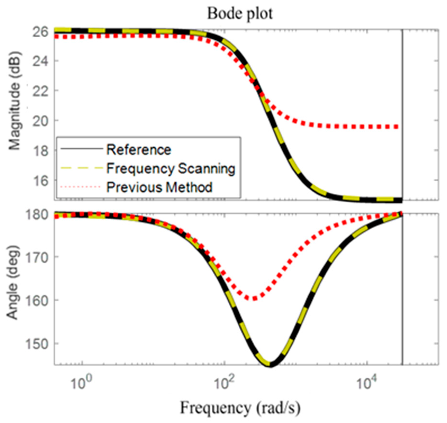
3.1. System Modeling and Verification
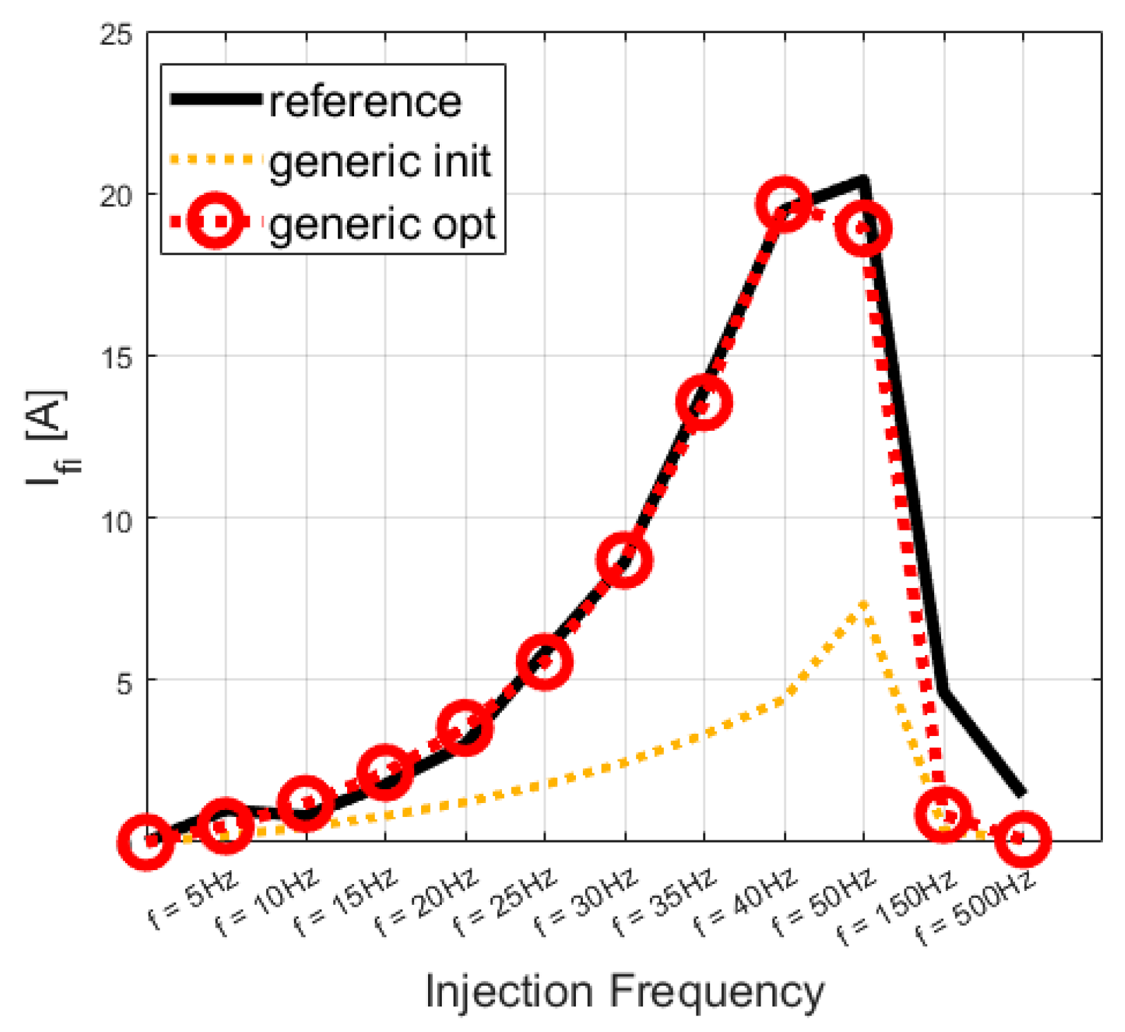
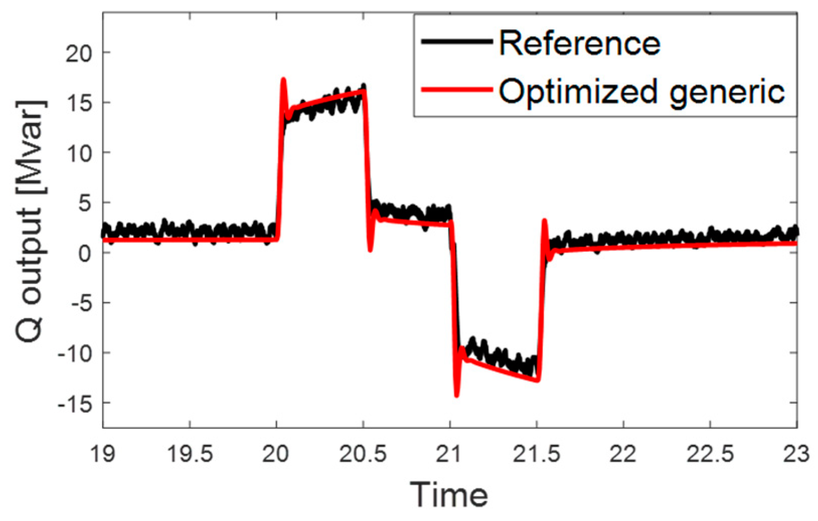
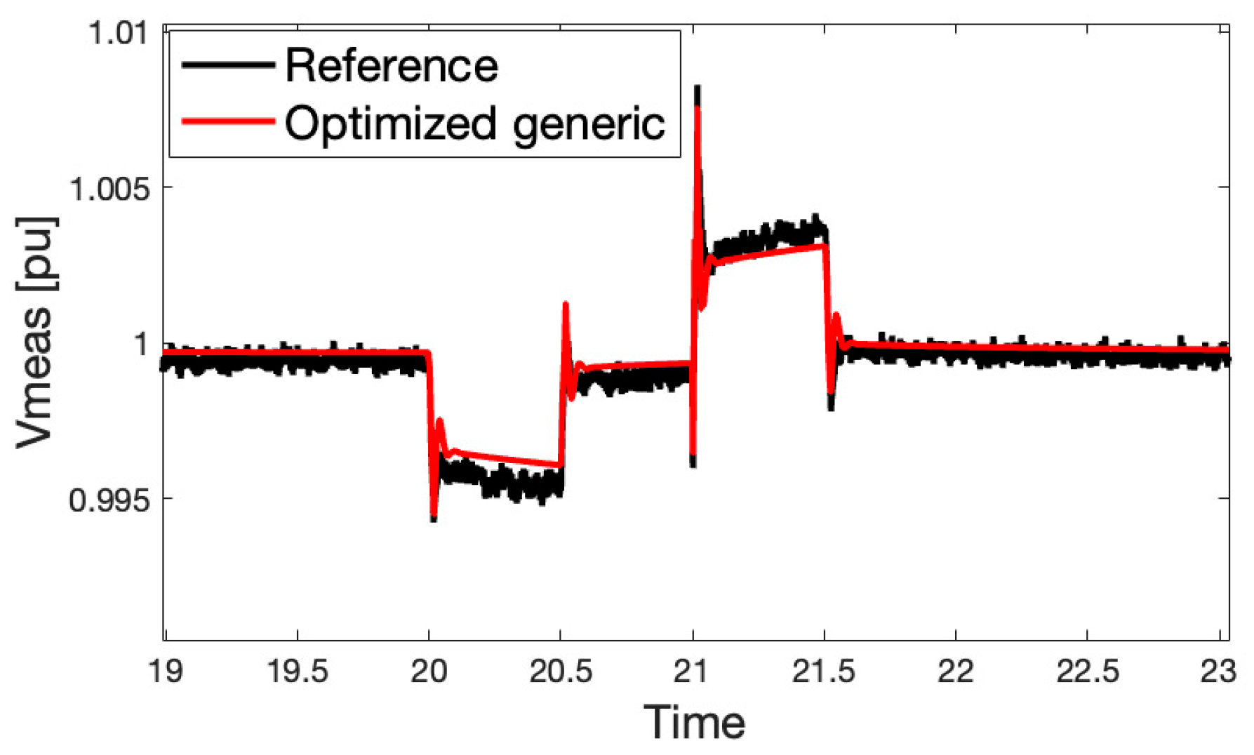
3.2. Using the Generic Model as a Reference
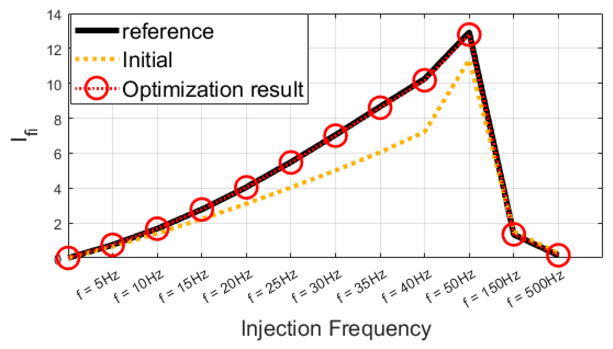
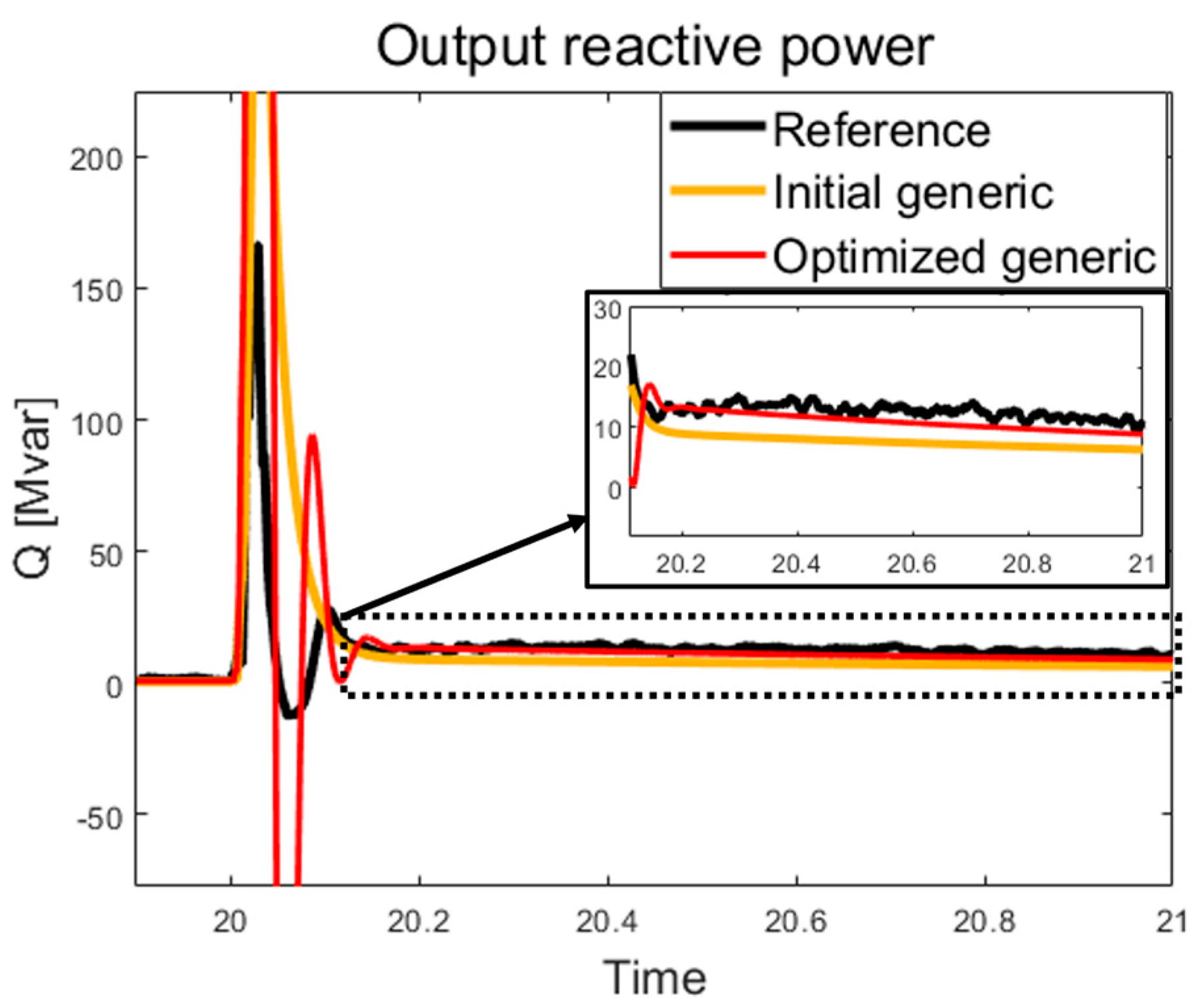
3.3. Using the Switching-Based Model as the Reference
4. Conclusions
- To enable various analyses using the TSA program, the proposed method was validated with the TSA generic model as the reference, demonstrating improved generalizability compared to previous approaches.
- To verify the applicability of the proposed model when the reference model is provided as a switching-based black-box model, a validation process was conducted using a detailed model as the reference, confirming that the proposed model accurately replicates the reference model with high precision.
Author Contributions
Funding
Data Availability Statement
Conflicts of Interest
References
- Quintero, J.; Vittal, V.; Heydt, G.T.; Zhang, H. The Impact of Increased Penetration of Converter Control-Based Generators on Power System Modes of Oscillation. IEEE Trans. Power Syst. 2014, 29, 2248–2256. [Google Scholar] [CrossRef]
- Poulose, A.; Kim, S. Transient Stability Analysis and Enhancement Techniques of Renewable-Rich Power Grids. Energies 2023, 16, 2495. [Google Scholar] [CrossRef]
- Cole, S.; Beerten, J.; Belmans, R. Generalized Dynamic VSC MTDC Model for Power System Stability Studies. IEEE Trans. Power Syst. 2010, 25, 1655–1662. [Google Scholar] [CrossRef]
- Kwon, J.; Wang, X.; Blaabjerg, F.; Bak, C.L.; Sularea, V.-S.; Busca, C. Harmonic Interaction Analysis in a Grid-Connected Converter Using Harmonic State-Space (HSS) Modeling. IEEE Trans. Power Electron. 2016, 32, 6823–6835. [Google Scholar] [CrossRef]
- Zhu, Y.; Gu, Y.; Li, Y.; Green, T.C. Impedance-Based Root-Cause Analysis: Comparative Study of Impedance Models and Calculation of Eigenvalue Sensitivity. IEEE Trans. Power Syst. 2022, 38, 1642–1654. [Google Scholar] [CrossRef]
- Kwon, D.; Kim, Y. Analyses and Comparisons of Generic and User Writing Models of HVDC System Considering Transient DC Current and Voltages. Energies 2021, 14, 7897. [Google Scholar] [CrossRef]
- Cossart, Q.; Colas, F.; Kestelyn, X. Model reduction of converters for the analysis of 100% power electronics transmission systems. In Proceedings of the 2018 IEEE International Conference on Industrial Technology (ICIT), Lyon, France, 20–22 February 2018; pp. 1254–1259. [Google Scholar]
- Hu, W.; Wu, Z.; Dinavahi, V. Dynamic Analysis and Model Order Reduction of Virtual Synchronous Machine Based Microgrid. IEEE Access 2020, 8, 106585–106600. [Google Scholar] [CrossRef]
- Zhang, B.; Nie, S.; Jin, Z. Electromagnetic Transient-Transient Stability Analysis Hybrid Real-Time Simulation Method of Variable Area of Interest. Energies 2018, 11, 2620. [Google Scholar] [CrossRef]
- Ray, I. Review of Impedance-Based Analysis Methods Applied to Grid-Forming Inverters in Inverter-Dominated Grids. Energies 2021, 14, 2686. [Google Scholar] [CrossRef]
- Agnihotri, P.; Das, M.K.; Gole, A.M.; Jayasekara, B.; Muthumuni, D. Transient Simulation Based Model Identification of a Black Boxed LCC HVDC. In Proceedings of the 2018 Power Systems Computation Conference (PSCC), Dublin, Ireland, 11–15 June 2018. [Google Scholar]
- Filizadeh, S.; Gole, A.M.; Woodford, D.A.; Irwin, G.D. An Optimization-Enabled Electromagnetic Transient Simulation-Based Methodology for HVDC Controller Design. IEEE Trans. Power Deliv. 2007, 22, 2559–2566. [Google Scholar] [CrossRef]
- Ko, B.; Nam, S.; Koo, B.; Kang, S. A Study on Estimation of Facts Dynamic Model Parameters Using Pmu Data. Trans. Korean Inst. Electr. Eng. 2020, 69, 1149–1156. [Google Scholar] [CrossRef]
- Resende, F.O.; Lopes, J.A.P. Development of Dynamic Equivalents for MicroGrids using System Identification Theory. In Proceedings of the 2007 IEEE Lausanne Power Tech, Lausanne, Switzerland, 1–5 July 2007. [Google Scholar]
- Cifuentes, N.; Sun, M.; Gupta, R.; Pal, B.C. Black-Box Impedance-Based Stability Assessment of Dynamic Interactions Between Converters and Grid. IEEE Trans. Power Syst. 2021, 37, 2976–2987. [Google Scholar] [CrossRef]
- Zhao, F.; Wang, X.; Zhou, Z.; Harnefors, L.; Svensson, J.R.; Kocewiak, L.; Gryning, M.P.S. A General Integration Method for Small-Signal Stability Analysis of Grid-Forming Converter Connecting to Power System. In Proceedings of the 2020 IEEE 21st Workshop on Control and Modeling for Power Electronics (COMPEL), Aalborg, Denmark, 9–12 November 2020; pp. 1–7. [Google Scholar]
- Rygg, A.; Molinas, M. Apparent Impedance Analysis: A Small-Signal Method for Stability Analysis of Power Electronic-Based Systems. IEEE J. Emerg. Sel. Top. Power Electron. 2017, 5, 1474–1486. [Google Scholar] [CrossRef]
- Amin, M.; Molinas, M. Small-Signal Stability Assessment of Power Electronics Based Power Systems: A Discussion of Impedance- and Eigenvalue-Based Methods. IEEE Trans. Ind. Appl. 2017, 53, 5014–5030. [Google Scholar] [CrossRef]
- Sun, J. Impedance-Based Stability Criterion for Grid-Connected Inverters. IEEE Trans. Power Electron. 2011, 26, 3075–3078. [Google Scholar] [CrossRef]
- Nelder, J.A.; Mead, R. A Simplex Method for Function Minimization. Comput. J. 1965, 7, 308–313. [Google Scholar] [CrossRef]
- PSS®E 34.4 Model Library; Siemens Industry, Inc., Siemens Power Technologies International: Schenectady, NY, USA, 2018.
- MathWorks. Statcom Detailed Model. Available online: https://www.mathworks.com/help/sps/ug/statcom-detailed-model.html (accessed on 13 January 2025).
- Paolone, M.; Gaunt, T.; Guillaud, X.; Liserre, M.; Meliopoulos, S.; Monti, A.; Van Cutsem, T.; Vittal, V.; Vournas, C. Fundamentals of Power Systems Modelling in the Presence of Converter-Interfaced Generation. Electr. Power Syst. Res. 2020, 189, 106811. [Google Scholar] [CrossRef]


| CASE | T1 | T2 | T3 | T4 | KDROOP | X | KI |
|---|---|---|---|---|---|---|---|
| REFERENCE | |||||||
| INITIAL | |||||||
| RESULT |
| Reference System | Proposed Method | Previous Method | |
|---|---|---|---|
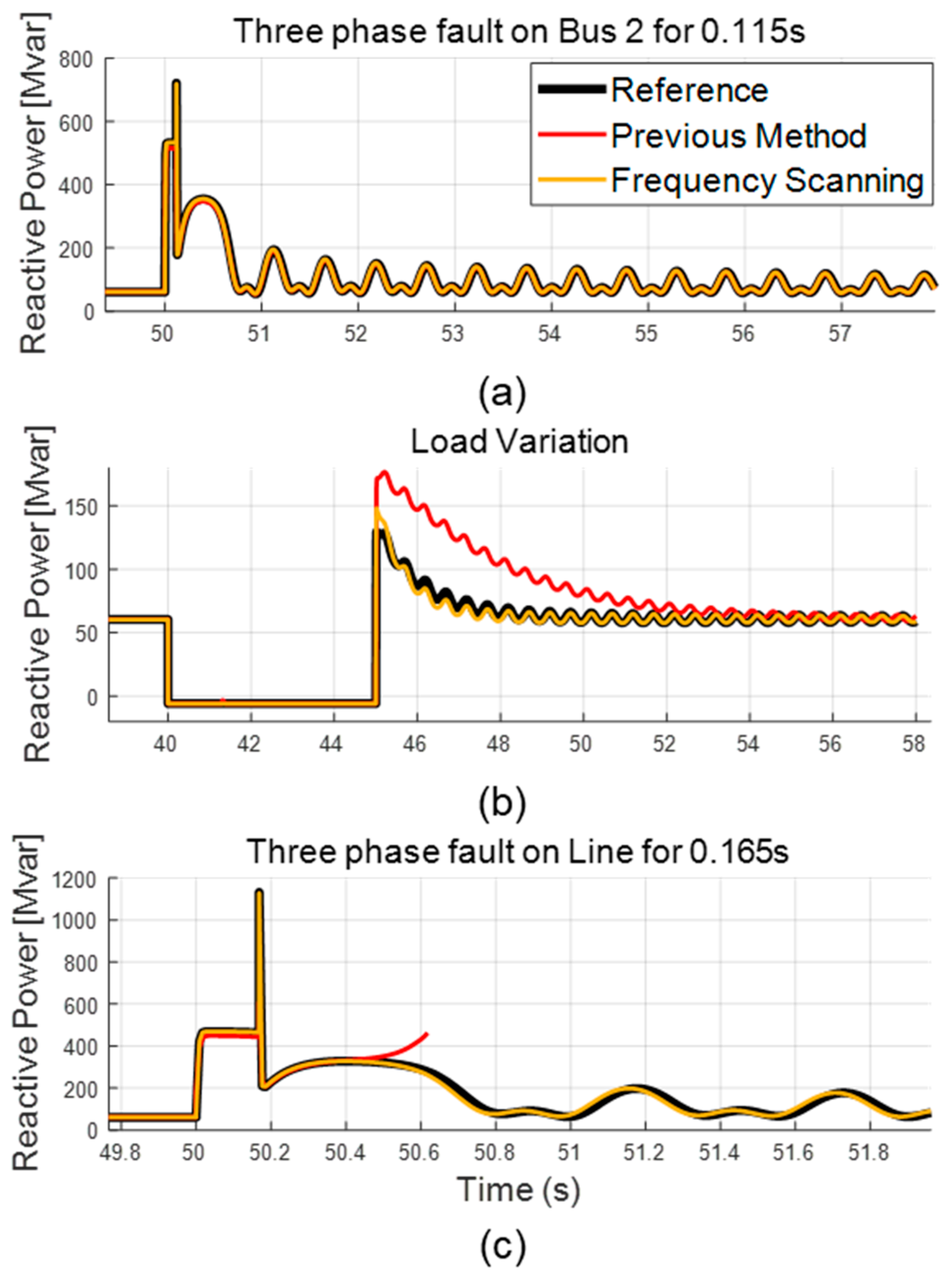
| Scenario Number | Scenario Description |
|---|---|
| 1 | Three-phase fault at bus 2 |
| 2 | Q variation at load 2 |
| 3 | Three-phase fault at bus 1–3 branch |
| Parameter Estimation Method | Settling Time [s] | Peak Q Value [Mvar] |
|---|---|---|
| Reference system | 47.87 | 129.63 |
| Proposed method | 47.34 | 148.02 |
| Previous method | 53.27 | 176.63 |
| T1 | T2 | T3 | T4 | Kdroop | X | Ki |
|---|---|---|---|---|---|---|
| Time [s] | ~20 | 20 | 20.5 | 21 | 21.5 |
|---|---|---|---|---|---|
Disclaimer/Publisher’s Note: The statements, opinions and data contained in all publications are solely those of the individual author(s) and contributor(s) and not of MDPI and/or the editor(s). MDPI and/or the editor(s) disclaim responsibility for any injury to people or property resulting from any ideas, methods, instructions or products referred to in the content. |
© 2025 by the authors. Licensee MDPI, Basel, Switzerland. This article is an open access article distributed under the terms and conditions of the Creative Commons Attribution (CC BY) license (https://creativecommons.org/licenses/by/4.0/).
Share and Cite
Jo, H.; Lee, J.; Kim, S. Frequency Scanning-Based Dynamic Model Parameter Estimation: Case Study on STATCOM. Energies 2025, 18, 1326. https://doi.org/10.3390/en18061326
Jo H, Lee J, Kim S. Frequency Scanning-Based Dynamic Model Parameter Estimation: Case Study on STATCOM. Energies. 2025; 18(6):1326. https://doi.org/10.3390/en18061326
Chicago/Turabian StyleJo, Hyeongjun, Juseong Lee, and Soobae Kim. 2025. "Frequency Scanning-Based Dynamic Model Parameter Estimation: Case Study on STATCOM" Energies 18, no. 6: 1326. https://doi.org/10.3390/en18061326
APA StyleJo, H., Lee, J., & Kim, S. (2025). Frequency Scanning-Based Dynamic Model Parameter Estimation: Case Study on STATCOM. Energies, 18(6), 1326. https://doi.org/10.3390/en18061326