Article

Evaluating Combustion Ignition, Burnout, Stability, and Intensity of Coal–Biomass Blends Within a Drop Tube Furnace Through Modelling

by
Garikai T. Marangwanda
1,2,* and
Daniel M. Madyira
1
1
Department of Mechanical Engineering Science, University of Johannesburg, Johannesburg 2026, South Africa
2
Centre of Applied Research and Innovation in the Built Environment, University of Johannesburg, Johannesburg 2026, South Africa
*
Author to whom correspondence should be addressed.
Energies 2025, 18(6), 1322; https://doi.org/10.3390/en18061322
Submission received: 3 February 2025 / Revised: 27 February 2025 / Accepted: 28 February 2025 / Published: 7 March 2025

Abstract

:
This study focused on evaluating the combustion ignition, burnout, stability, and intensity of Hwange coal and Pinus sawdust blends within a drop tube furnace (DTF) through modelling. The cocombustion of coal with biomass is gaining attention as a strategy to improve fuel efficiency and reduce emissions. Hwange coal, a key energy source in Zimbabwe, produces significant emissions, while Pinus sawdust offers a renewable alternative with favourable combustion properties. Optimising cocombustion performance is highly dependent on understanding various mass- and energy-conservation-related parameters in detail, hence the motivation of this study. The fuels of interest were blended through increasing the Pinus sawdust mass percentages up to 30%. A DTF that is 2 m long and 0.07 m in diameter was modelled and validated successfully using particle residence time and temperature profiles. An increase in blending resulted in an increase in combustion intensity, as made apparent by the heat of reaction profiles, which were also shown to be dependent on the kinetic rate of the reaction between CO and O2 to form CO2. The burnout rate profiles demonstrated that as blending increased, heat was released more abruptly over a short distance; hence, combustion became less stable. The burnout rate profiles were shown to be dependent on the kinetic rate of reaction between char and O2 to form CO. The effect of DTF wall temperatures (1273, 1473, and 1673 K) was also studied, with the results showing that at a low temperature, the reaction zone was delayed to a distance of 0.8 m from the injection point, as compared to 0.4 m at 1673 K. In summary, this study demonstrated that combustion ignition, burnout, and intensity increased with the blending ratio of Pinus sawdust, whilst combustion stability decreased.

1. Introduction

The cocombustion of coal with biomass waste has been under investigation for a long time with the main aim of reducing emissions traditionally obtained from coal combustion on its own [1]. Varied experimental techniques ranging from pilot-scale to actual power plant combustion scenarios have been studied over the years with success [2,3]. With the continued developments in technology, the modelling of cocombustion has also taken a prominent role as engineers seek to optimise the combustion process by extracting maximum energy and maximum waste incineration at reduced emissions and minimum cost [4,5]. Some researchers then saw it fit to characterise the change in combustion parameters from a technical point of view, thus studying the influence of cocombustion on burnout, ignition, stability, and intensity [6]. Being able to predict the influence of cocombustion on various combustion parameters is of practical importance to furnace operators in industry. Good and predictable ignition properties imply that combustion reactions commence within the expected time range, thus avoiding problems caused by premature or delayed ignition [7]. Consequently, the energy absorbed from the furnace to offset ignition is accurately predicted, leaving furnace operators with useful optimum operating parameters.
Burnout can be described as the ability of a fuel sample to extinguish its combustible material, which includes the volatile matter and char constituents. With respect to solid fuel combustion, most researchers monitor burnout in the same manner by measuring the char content only at the furnace exit in comparison to the initial fixed carbon content [7]. Benim et al. [2] during their studies with pre-dried lignite and torrefied biomass and Gao et al. [8] during their studies with Colombian coal and woodchip directly or indirectly showed improvement in the overall burnout as blending increased when they monitored the char content in the products. It is important not to overlook the homogenous gaseous combustion products when analysing burnout since carbon monoxide and other unburnt gaseous constituents also influence the overall burnout percentage [9]. Some heavy volatile components released during the devolatilisation process of solid fuels require relatively long residence times to attain complete combustion [10]. As far as the researchers are concerned, no CFD studies have been reported that have managed to monitor both carbon in ash and carbon monoxide in flue gases concurrently as a function of burnout percentage.
The application of mass conservation towards cocombustion entails looking at the quantity and composition as well as the rate of production or depletion of combustion species. By extension, the validation of a cocombustion model is usually based on measuring the species molar fraction along and across the furnace. The application of energy conservation towards cocombustion modelling entails monitoring temperature-related parameters. The basic parameters that are mainly used for cocombustion model validation are temperature and wall heat flux [11]. Of equal importance, but less alluded to during the combustion modelling of boilers, are flame stability and intensity. Combustion stability, a measure relatively linked to ignition and homogenous combustion, is generally used to monitor the predictability of a combustion process [6]. When fuel blending is being monitored, it is imperative that stability is maintained to avoid any flashback or liftoff flames or, in extreme cases, flame extinction [12]. Ma et al. [13] monitored the heat flux profiles that are exhibited by blended samples, which can be used to evaluate combustion stability and intensity. To be more accurate, it makes sense to monitor combustion stability through plotting rate of heat release profiles, as residence time is also incorporated into the analysis. It is expected that homogeneous volatile combustion is less stable compared to heterogeneous char combustion, which means that highly blended samples are less stable when comparing the activation energy required in each case [14,15].
Interestingly, the lesser the stability, the higher the combustion intensity, which is closely linked to the heat released, as demonstrated by Marangwanda et al. [6] during their studies with coal and sawdust. As far as experimental procedures are concerned, the use of image processing techniques will likely give a complete understanding of flame behaviour, which can help with the evaluation of combustion intensity. Unfortunately, most of these experimental procedures require specialised equipment [16,17].
Table 1 summarises different modelling studies that have been carried out and how they reported on ignition, burnout, intensity, and stability. The ability to capture almost all of these combustion parameters by CFD makes it an indispensable and affordable tool with regard to cocombustion optimisation. This study addresses the gap existent with regard to combining most of these combustion parameters whilst optimising the cocombustion process.

2. Experimental Methods

2.1. Fuel Blend Characterisation

The physical and chemical fuel specifications of the fuel blends of interest have been detailed in a prior publication by the same authors [22]. Hwange coal, a bituminous thermal-grade coal, is widely used in Zimbabwe’s power generation due to its high availability and established infrastructure for extraction and utilisation. However, its combustion leads to significant greenhouse gas emissions, making it necessary to explore alternative co-firing strategies. Pinus sawdust, on the other hand, is an abundant waste biomass in Zimbabwe, primarily sourced from sawmill operations in the Eastern Highlands. Its high volatile matter and lower sulphur content make it a suitable candidate for cocombustion with coal, contributing to emission reduction and improved combustion characteristics [6,22]. Using the fuel characterisation results, the volatile composition for each blend was determined. It was assumed that each volatile had a lumped form represented by CaHbOcNdSe regardless of the various constituents of volatiles such as CH4, CO, etc. Using proximate, ultimate, and calorific experimental data, the lumped volatile composition for each fuel blend was derived through analytical methods [23], as demonstrated by the equations in Table 2.
Here, VM and FC represent volatile matter and fixed carbon, whilst the subscript daf denotes “dry ash free”. C, H, N, S, and O represent carbon, hydrogen, nitrogen, sulphur, and oxygen. To determine the enthalpy of formation for the volatile (Hf,vol), Equation (3) was employed after rearranging Equations (1) and (2).
H f , fuel =   FC daf × H f , char + VM daf × H f , vol
H f , char :   C + O 2 = CO 2   32.8 MJ / kg ;   H f , char = LCV coal
H f , char = LCV coal = HCV coal h latent , H 20 × MC ar 1 MC ar Ash ar H ar × Mr H 2 O 2 × Mr H × h latent , H 20
This method offered a more comprehensive approach to representing fuel properties, avoiding the assumption that the fuel sample consists solely of methane or butane, as suggested by some authors [24,25]. The proximate and volatile compositions of the blends that were used are presented in Table 3.
The molar ratio of carbon showed an increase with blending from 0.292 up to 0.579 for a 30% blending ratio, as summarised in Table 3. Similar trends were also experienced with hydrogen and oxygen though to a lesser magnitude. Nitrogen in the volatile decreased with blending from 0.086 to 0.052 as blending increased, whilst the sulphur content decreased marginally with blending. This is supported by other authors indirectly through the assertion that biomass contains higher volatile matter than coal. This translates to a gradual decrease in energy content since the H/C ratio of blended volatiles is lower than that of the unblended sample [26]. Maisyarah et al. [27] also suggested that a lower H/C ratio tended to result in a higher mass loss for the overall sample at the end of the combustion process. As such, a higher mass loss was expected for the blended fuel samples. The kinetic parameters of the fuel blends as obtained from thermogravimetric analysis are summarised in Table 4, representing the homogenous (volatile) and heterogenous (char) combustion stages. Detailed information about kinetic parameter determination is available in a previous paper by the same authors [22].

2.2. Drop Tube Furnace Experimental Setup

The drop tube furnace (DTF) experimental setup consisted of an alumina tube serving as the furnace, with a total height of 2032 mm and an internal diameter of 70 mm. A detailed description of the setup and procedure is available in the work of Marangwanda and Madyira [28]. The furnace had an alumina silicate refractory lining, with heating tubes systematically positioned around the alumina tube. Fuel blends were introduced through a 2 mm cooled injector at 373 K, while a 6 mm cooled sampling probe at the reactor exit facilitated collection. Within the fuel feeding system, 15 g of fuel blends was placed in a test tube, which was connected to the primary carrier gas flowing at an average rate of 2.5 NL/min (within a 1.5–3.5 NL/min range). An electromechanical vibrator enabled controlled fuel feeding, ensuring fluidisation by the primary carrier gas, which transported the fuel into the outgoing pipe leading to the furnace. The water-cooled sampling probe maintained a suction flow rate of 6–15 NL/min, while the secondary gas was preheated to 1273 K and supplied at 10–20 NL/min, depending on the required furnace residence time. The collecting probe was positioned at variable distances 520 mm, 920 mm, and 1320 mm along the furnace centreline at pre-determined experimental conditions. A bag filter was located at the outlet such that char and ash could be collected for subsequent analysis.
During devolatilisation, the system operated at a single set temperature of 1273 K, whereas during char combustion, three furnace temperature settings (1273 K, 1473 K, and 1673 K) were investigated. The injector was modelled to introduce fuel in a normal direction to the inlet, making an assumption that no swirl effects existed. The experimental procedure was conducted in two distinct stages. The first stage was performed under a nitrogen atmosphere, simulating the devolatilisation process, while the second stage took place in an oxygen-enriched environment, representing char combustion. During the first stage, only solid char was collected and analysed, as the released volatiles were carried away with the exhaust gases. Given that devolatilisation requires short residence times, a 520 mm probing position was deemed adequate for data collection. Following char collection and characterisation, the second stage involved reintroducing the char into the DTF under an oxygen-enriched atmosphere (3% O2, 97% N2), leading to the final production of ash. The use of a two-stage approach was necessitated by DTF operating temperature limitations and combustion atmosphere constraints. A controlled 3% O2 concentration ensured the development of gradual combustion profiles suitable for this study. Higher O2 concentrations tend to accelerate combustion reactions, potentially leading to intensified reaction zones or even explosive conditions, making precise measurement difficult with the available instrumentation.
These observations were experimentally demonstrated by Zou et al. [29] whilst studying the combustion of pulverised coal under various atmospheres ranging from 21% to 50% O2.
Within a DTF, the fuel is exposed to an isothermal heating rate within the range of 104 and 105 K/s, which is quite high when compared to any TGA analysis. Liu et al. [30] studied the cocombustion kinetic parameters of biomass and plastic at high heating rates within the range of 104 K/s. Their findings demonstrated that in as much as combustion parameters vary by large factors when the heating rate increases, kinetic parameters such as the activation energy and pre-exponential factor succumb to the compensation effect at high heating rates. The heating rate increased with activation energy at first; it then decreased and eventually remained at the same value for heating rates of 750 and 1000 K/min. However, Czajka et al. [31], whilst extrapolating the kinetic parameters of South African coal during the pyrolysis process, suggested using corrections, as given in Equations (4) and (5).
k heat 1 k heat 2 = A heat 1 A heat 2 n = β heat 1 β heat 2 n
A heat 1 β heat 1 = ϑ 1 . e x p ( ϑ 2 . E )
where k denotes the kinetic rate, β is the heating rate, n is a factor dependent on the amount of weight released, heat1 and heat2 refer to parameters at the 1st and 2nd heating rates, and ϑ is a parameter which is closely related to the compensation effect [32]. Through inference from their findings, the authors determined the corresponding kinetic parameters for DTF simulation. As noted, during the first stage of the experiment, which was conducted under a nitrogen atmosphere, the released volatiles were entrained in the carrier gas, while the solid char was collected using a bag filter at the outlet. In the second stage, which was under an oxygen-enriched atmosphere, the char underwent complete combustion, leaving behind ash, which was collected at the outlet as well. The properties of the particles that were not directly measurable were estimated indirectly using experimental data, which included the use of fluid velocity and particle size distribution.

3. Numerical Methods

ANSYS FLUENT 2021 R1 was used to implement the cocombustion model that had been developed which is based on the conservation equation, as given in Equation (6) [33].
t ρ φ + x i ρ U i φ = x i Γ φ x i + S φ
where the following variables are used:
  • ρ: represents the density;
  • φ: variable (mass, specific enthalpy, or species mass fraction);
  • Ui: velocity (u, v, w);
  • Γ: variable diffusion coefficient;
  • Sφ: variable source or sink.

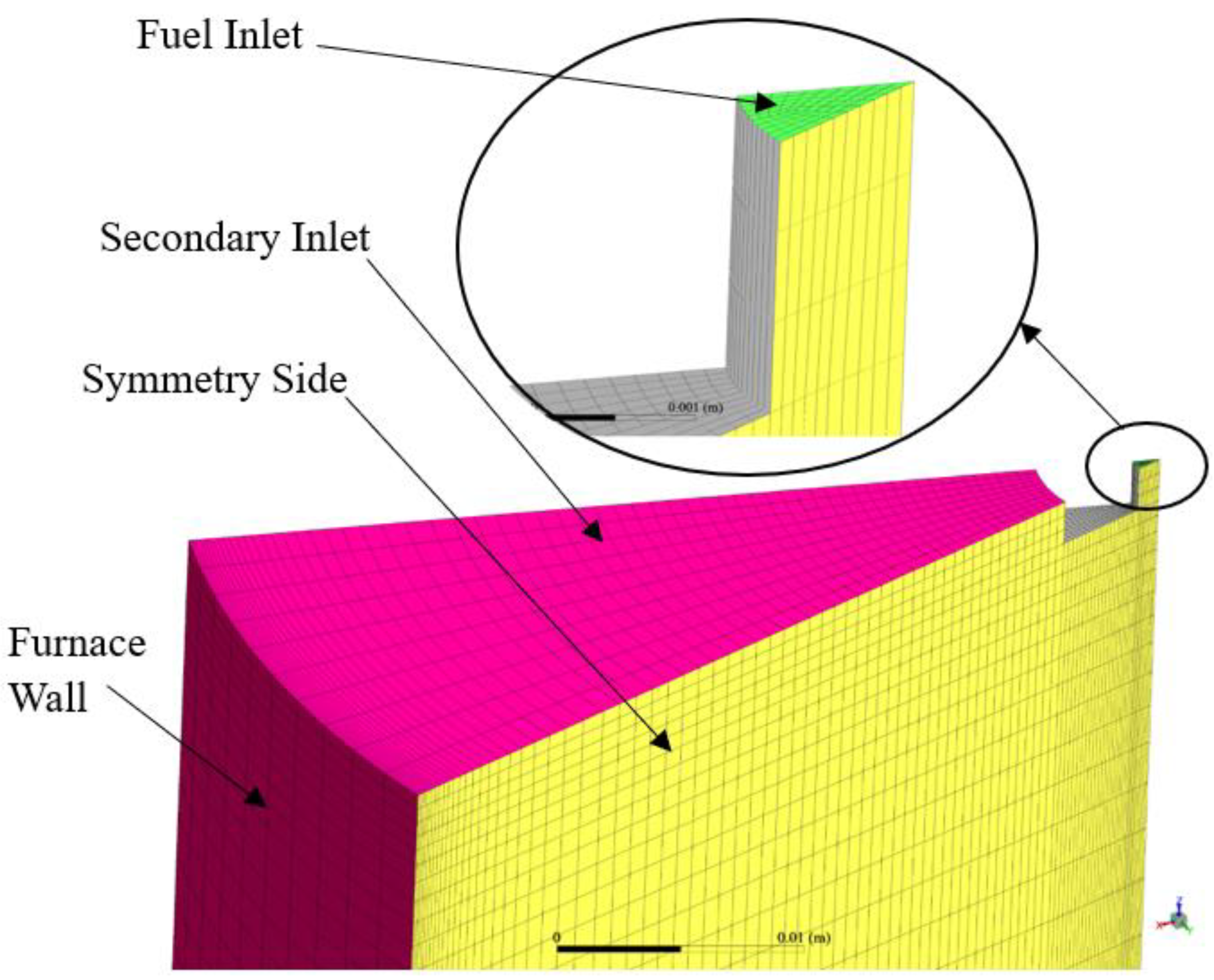
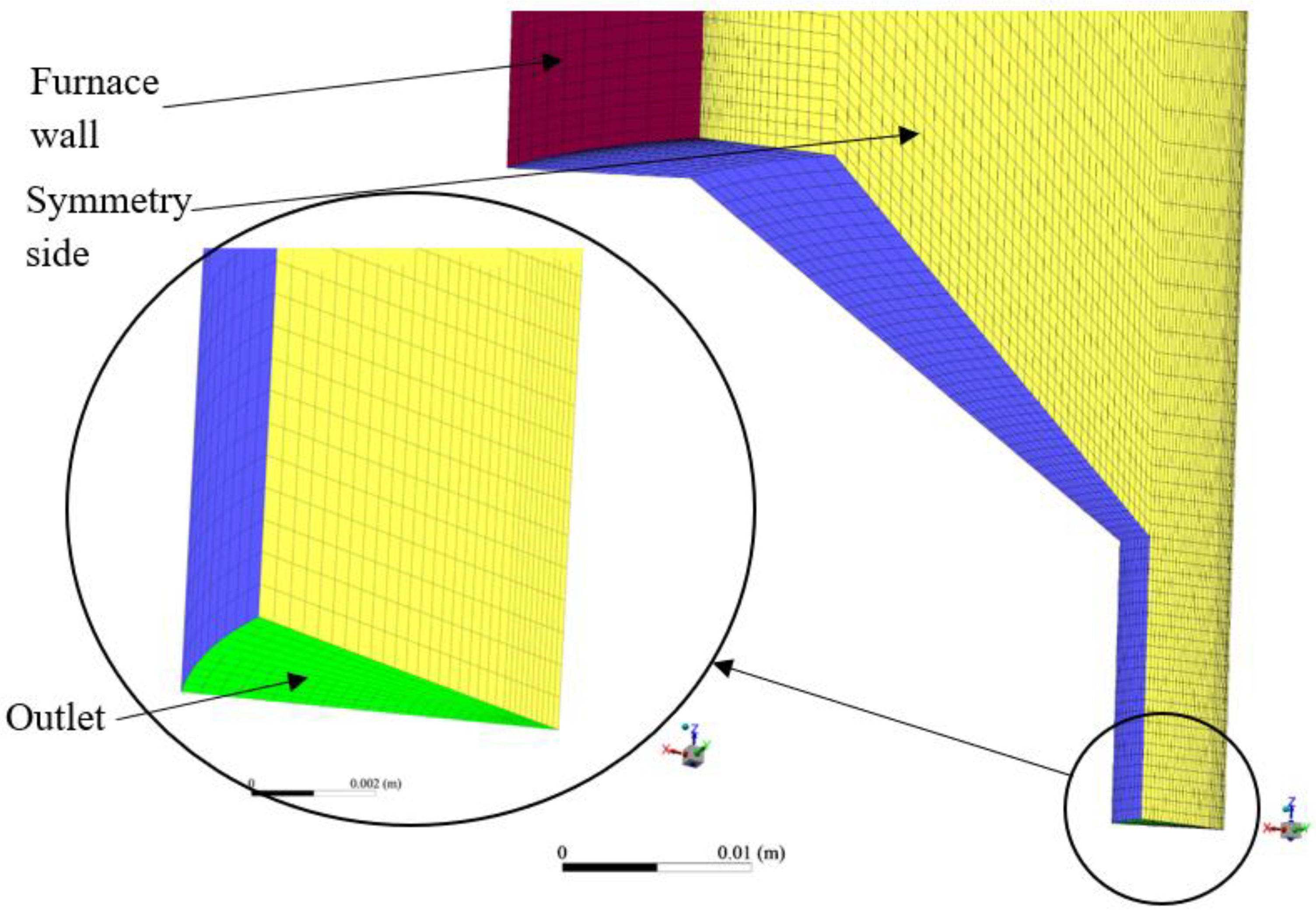
3.1. Furnace Geometry and Meshing

The boundaries drawn and meshed were simplified to only capture the important physics that influence the combustion process.
Since the experimental DTF had a cylindrical shape, only 30° of the DTF was modelled due to the following:
  • There was a need to reduce the computational power required to run the setup;
  • The geometry was cylindrical about the furnace axis;
  • A 3D analysis would be able to capture the axial and radial variation in parameters with more precision as compared to a 2D analysis;
  • The inlets (fuel inlet and secondary carrier gas inlet) and outlet boundaries were all normal to the symmetrical planes that were defined;
  • The expected flow was going to be repeated periodically about the axis since the fuel and secondary carrier gas inlet flows were distributed evenly and normal to their corresponding boundaries.
A structured mesh was employed for the furnace meshing; thus, hexa-meshing was performed. During meshing, emphasis was placed on achieving acceptable determinant (>0.2), angle (>18°), and warpage (<10) values for all the meshes that were generated so as to reduce any errors associated with bad meshing in the later stages. All the structured meshes had some wall inflation to capture the boundary layer and a bit of refinement towards the axis to anticipate the reaction zone position. Illustrations of the meshing employed within this study are given in Figure 1 and Figure 2.

3.2. Cocombustion Model Setup

The submodels that were used to capture combustion were compiled within ANSYS FLUENT 2021 R1. The main strength of ANSYS FLUENT 2021 R1 with regard to combustion modelling lies within its ability to handle user-defined functions (UDFs). UDFs allowed the researchers to include customised submodels other than those built in by default within ANSYS FLUENT 2021 R1. Due to their versatility and conciseness, C++ codes were written to act as the UDFs for incorporation into the ANSYS FLUENT 2021 R1 overall combustion model. The UDFs were used to customise mainly the furnace freeboard temperature profile, particle drag properties of the coal and biomass species as they travelled through the furnace, and specific heat capacities of the various participating gaseous species such as CO2, N2, O2, and H2O. Table 5 summarises the boundary conditions that were employed by the researchers.
The sawdust particles utilised a shape factor of 0.83 since a cylindrical shape was assumed due to the fibrous nature of biomass. In as much as the pulverised Hwange coal particles were irregular in shape, they were assumed to be spherical because when small coal particles heat up, they tend to soften up and adopt a spherical shape [26].
Since the first stage was carried out under a nitrogen-enriched atmosphere, resembling the devolatilisation process, the main chemical reactions that were expected were related to the release of volatiles. As already investigated under the TGA experiments, devolatilisation was deduced to follow the single-rate kinetic devolatilisation submodel, as given in Table 4. The second stage was carried out under a 97% nitrogen and 3% oxygen atmosphere, resembling the heterogenous combustion of char. No homogenous combustion of volatiles was expected because all the volatiles were carried along with the carrier gas in the first stage and, thus, were not present during the second stage. The heterogenous surface reaction mechanisms are also known as multiple surface reaction mechanisms because the reactions are assumed to take place within the boundary layer and bulk flow simultaneously. The activation energy and pre-exponential factors during heterogenous combustion are given in Table 4, as determined by the researchers using TGA experiments. The gasification reactions of char with CO2 or H2O were overlooked since the reaction temperatures within the reactor were not high enough to warrant their influence. Furthermore, the concentrations of CO2 and H2O were low as compared to N2 [34].
The furnace was calibrated using a different coal sample to verify the effectiveness of the thermal measurements. In as much as the furnace wall was set to have a certain temperature, the actual furnace wall temperature was slightly different from the setting, as shown in Figure 3. A known fuel sample made of South African coal was used to calibrate the furnace and validate the cocombustion model. Table 6 summarises the chemical properties of the South African coal used for furnace calibration and validation.

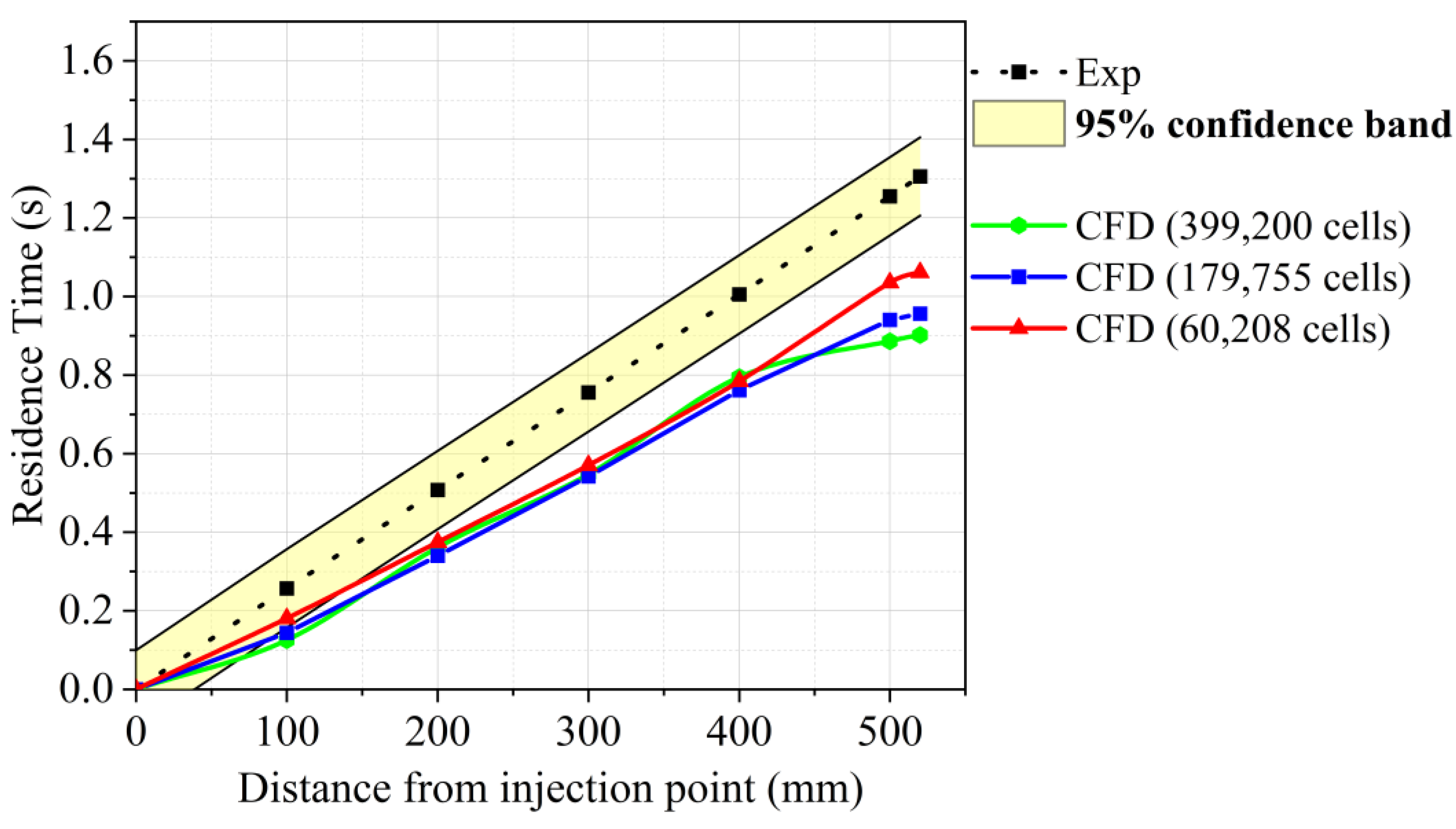
3.3. Drop Tube Furnace Model Sensitivity Analysis

The grid convergence index (GCI), as propounded by Roache [35], looks at the effect of mesh density on the variation in performance parameters. This index is adapted for fluid-based analysis through its ability to analyse boundary layer effects by the use of near-wall inflation monitoring. Only the GCI analysis was conducted, as it was deemed enough to analyse the combustion parameters under consideration. More focus was placed on the near-wall inflation parameters, hence the GCI. The performance parameters were those variables of interest to the user during the modelling practice. As such, mesh independence was achieved when the index approached unity. In this case, the particle final residence time and particle peak temperature were used to evaluate the GCI. As illustrated in Figure 1 and Figure 2, the shortest edge had a distance of 1.109 mm, which was used to guide the initial seed element size for the course mesh.
Refinement was then carried out depending on the required emphasis, as presented. The 399,200-cell mesh (mesh 1), 159,755-cell mesh (mesh 2), and 60,208-cell mesh (mesh 3) were evaluated to give a refinement ratio (r) of around 2.576. Equations (7) to (10) were thus employed to evaluate the GCI based on the parameters of interest, as presented in Table 7.
p = ln f 3 f 2 f 2 f 1 / ln ( r )  
GCI 12 = F s × f 2 f 1 f 1 r p 1
GCI 23 = F s × f 3 f 2 f 2 r p 1
GCI 23 r p ×   GCI 12 1
where the following variables are used:
  • p: order of convergence;
  • f: performance parameter;
  • r: refinement ratio = 2.576;
  • GCI: grid convergence index;
  • Fs: factor of safety (in this case, 2 levels of refinement = 1.25).
As illustrated in Table 7, the asymptotic range values are both within the range of unity, highlighting how the solution is mesh-independent for the three meshes under consideration. Potgieter et al. [36] made a similar conclusion with regard to the grid convergence index during their heat transfer studies, which further supports the robust nature of this approach.
Table 7. Mesh sensitivity based on grid convergence index.
Mesh CellsMesh LabelPerformance ParameterpGCI1GCI2Asymptotic Range Value
[Particle residence time (s)]
399,20011.29910.49860.09320.15651.0471
159,75521.2407
60,20831.3343
[Particle peak temperature (K)]
399,20011006.141.18400.01370.04130.9778
159,75521029.03
60,2083958.85
Figure 4 shows a trace of the average particle residence time as it passes through the furnace for the South African fuel sample under a 1273 K furnace temperature with a 520 mm probing position setting. All CFD meshes demonstrated a good initial estimation of particle residence time up to around 250 mm from the injection point. Eventually, the course mesh (60,208 cells) produced the least deviation from the experimental values by staying closer to the 95% confidence band up to the furnace exit.
In conclusion, mass conservation suggested the use of a medium-density mesh, whilst analysis based on energy conservation suggested the use of a course-density mesh. Correlation with the experimental parameters suggested the use of the course mesh; thus, all subsequent analysis employed a mesh density similar to the course mesh.

3.4. Cocombustion Model Validation

The char produced during stage 1 was then passed through the DTF under an oxidative atmosphere of 0.3% O2 and 97% N2. As expected, this triggered oxidation reactions as far as the char particle is concerned; hence, the experimental results related to the oxidation of SA coal char were subsequently used to validate the model further with respect to the particle residence time and particle temperature. The stage 2 setup allowed for extra probing positions at 520 mm, 920 mm, and 1320 mm from the fuel injection point. The stage 2 setup also allowed the researcher to investigate the effect of the heating rate as the SA char particle moved through the DTF by having different furnace wall temperatures of 1273, 1473, and 1673 K. Data obtained on the variation in the experimental and predicted residence time with respect to the position when the char from the SA coal sample was combusted within the DTF are presented in Table 8 and Figure 5.
The predicted values produced a similar trend as compared to experimental values, though an overprediction was experienced at all probing positions. A furnace temperature of 1273 K allowed the combusting particles to have a predicted residence time of 1.523 s when probed at 520 mm from the injection point. As the particle moved further within the furnace, the residence time increased to 4.755 s when probed at 1320 mm from the injection point. When compared to experimental residence times, a deviation of 17.05% was experienced at a 520 mm probing position. A deviation of 48.60% was experienced at a 1320 mm probing position. Averaging these deviations in the predicted particle residence times against the experimental residence times resulted in a root mean square error (RMSE) of 1.117 for a furnace temperature of 1273 K.
An increase in the DTF heating rate through an increase in the furnace temperature resulted in a decrease in the deviation between the experimental and predicted particle residence times. A furnace temperature of 1673 K resulted in a predicted particle residence time of 1.083 s at a probing position of 520 mm compared to an experimental value of 1.000 s, which represents a deviation of 8.30%. At a probing position of 1320 mm, the predicted particle residence time was 2.977 s compared to an experimental value of 2.500 s, representing a deviation of 19.08%. Similarly, averaging the deviations between the experimental and predicted values at a furnace temperature of 1673 K showed an RMSE value of 0.557.
The overprediction can be attributed to various factors related to the determination of the experimental particle residence time. The experimental particle residence time was determined indirectly through experimental measurements of fluid velocity and temperature at various positions. The evaluation of the experimental particle residence time assumed a constant particle diameter and density, though in reality, combustion causes a loss in mass for the char particle. This, in turn, gave a semblance of a heavy particle, whilst in reality, it is lighter in weight. Consequently, the terminal velocity was skewed to appear as if the particle was moving fast, which is far from reality (DTF used downward firing; thus, particles moved in the same direction as gravitational force).
Secondly, the drag model that was employed during CFD prediction is based on Haider and Levenspiel [37], whilst that used in the experimental determination is anchored on a constant derived from Stokes’ Law. This allowed the prediction model to capture the drag induced by an irregular-shaped particle, unlike the approach used in the experimental determination. Lastly, the deduction used for the experimental particle residence time assumes that all particles travel in a one-dimensional direction without any recirculation. This, in turn, overlooks the effect of the recirculation and three-dimensional movement of particles, as utilised by the CFD model. Thus, the overprediction of particle residence time is justified and within the acceptable range for the predicted and experimental values.
As the fuel particle travelled through the furnace, the experimental and predicted values of particle temperature were also evaluated for validation purposes. Table 9 and Figure 6 summarise the experimental and predicted results. As the combusting particles travelled through the DTF, comparison between the experimental and predicted particle temperatures demonstrated a reduction in deviation. At a furnace wall temperature of 1673 K, the combusting particle attained an experimental temperature of 1676.80 K compared to a predicted value of 1289.18 K when probed at a distance of 520 mm from the injection point. This represented a negative deviation of 23.11%. When probed at 1320 mm from the injection point, a positive deviation of 4.79% was experienced between the experimental particle temperature of 1511.19 K and the predicted value of 1583.59 K. Monitoring these deviations at various probing positions showed that when the DTF is under a high heating rate, the RSME attains its lowest value of 0.1422. This is mirrored by the RSME values for the particle residence time, which also show better prediction as the furnace wall temperature increases.
The deviation between the experimental and predicted particle temperature values can be attributed to the manner in which the experimental particle temperatures were determined. The experimental particle temperatures were not determined directly but rather through experimental furnace wall temperatures and equations related to the theory of char combustion. One of the steps used to determine the experimental particle temperature involved the use of a single-step mechanism to represent the oxidation of char. The single-step mechanism stipulates that char oxidises to CO2 without any formation of intermediate species. This notion contradicts what other researchers such as Zhou et al. [38] and Graeser et al. [39], who investigated coal char under different operating conditions, have suggested. As such, the cocombustion model employed the two-step mechanism which also catered for particle diffusion, conductivity, variable specific heat capacity, and the change in char porosity during the combustion process. In summary, the cocombustion model did manage to predict the char combustion of SA coal at different furnace temperatures with success. Measuring combustion parameters during drying, devolatilisation, char combustion, and volatile combustion is very difficult and largely dependent on sophisticated instruments since the residence time is very small. In as much as Table 9 and Figure 6 demonstrate deviations between the experimental and CFD temperature parameters, the trends correspond to each other. As articulated by Zhang et al. [40], at high heating rates, such as those encountered within a DTF, the validation of combustion models using experimental values tends to be centred around verifying if the trends correspond rather than obtaining accurate values.

4. Results and Discussion

Due to the release of heat during combustion, parameters related to the conservation of energy were monitored in detail for the different fuel blends using the developed cocombustion model (100HC, 90HC10PS, 80HC20PS, and 70HC30PS). These parameters included the particle temperature, sensible heat of the reaction, absolute heat of the reaction, and ignition, as well as the burnout properties. The heat released during char oxidation was modelled as a two-step reaction by assuming the formation of CO within the boundary layer and its subsequent oxidation to CO2 in the bulk flow. Since coal char had a higher combustible fraction than sawdust char, as demonstrated in a publication by the same authors [22], more heat was expected from the unblended sample. Figure 7 shows the particle temperature of the 100HC case as well as the 70HC30PS case when combusted in the DTF with a wall temperature of 1473 K. Blending did not result in any significant variation in the particle temperatures along the axis or radially. One of the main characteristics that influences solid fuel combustion is surface area. The particle sizes that were employed were relatively small to warrant influence due to size difference. Mandø et al. [41] suggested that pulverised samples adopt a quasi-similar spherical shape during combustion unlike large particles, which was demonstrated in this study. Blending was performed on a mass basis; thus, the fuel flow rates that were employed were constant regardless of fuel blending.
With the small flow rates that were employed in this study, furnace wall temperatures rather than combustion reactions were able to influence the particle temperature, as demonstrated in Figure 8. The figure demonstrates the influence of having a DTF wall temperature of 1673 K and 1273 K on the combustion of a 70HC30PS fuel sample. As the flow developed in an almost similar fashion, the particles under a high DTF wall temperature were able to attain higher values along the axial direction. Correlating with Figure 9, which shows species molar fractions of CO2 at various DTF wall temperatures, it is evident that particle temperature plays an important role in aiding the formation of CO2, as higher temperatures promote the formation of CO2.
With respect to the heat released, Figure 10 shows heat of reaction contours along the axis and radially for the 70HC30PS case as a function of furnace temperature. Since the oxidation of char is treated as a two-step reaction, the contours of the kinetic reaction rates were also superimposed on the figures for better analysis. The setting up of the cocombustion model had to resemble the experimental conditions, which required an artificial atmosphere containing 97% N2 and 3% O2 by volume; Equations (11) and (12) were employed after assuming a 100% excess O2 scenario. This was deduced through calculating the average experimental O2-to-fuel ratio for the various fuel blends.
C + 0.5   O 2 + 32.333   N 2 CO + 16.167   N 2
CO + 1.0   O 2 + 32.333   N 2 CO 2 + 32.333   N 2 + 0.5   O 2
The high N2 content in the products of combustion due to the artificial atmosphere resulted in a reduced heat of reaction for all the cases. This can be attributed to the fact that N2 has a higher specific heat capacity than O2. This allows N2 to absorb more heat than O2 just to raise the temperature by a unit temperature [42]. By correlating with Figure 11, which shows discrete-phase particle burnout superimposed with contours of the Equation (11) kinetic rate of reaction, it becomes quite evident that most of the heat was released during the oxidation of CO. The initial heat released during char oxidation corresponded to the particle burnout profiles. Low DTF wall temperatures reduced the heat of the reaction, as shown in Figure 10. As expected, low DTF wall temperatures hindered the oxidation of CO to form CO2, thus delaying the reaction zone to an average location of 0.8 m from the injection point as compared to the initial 0.4 m obtained at high furnace temperatures. The nature of the flow development resulted in a reaction zone that tended to be concentrated towards the centreline for high temperatures and near walls for low temperatures. The sensible heat released during combustion increased with temperature, as shown in Figure 12. As already discussed, high furnace temperatures increased the subsequent kinetic reaction rate associated with char oxidation and the heat of the reaction.
The effect of blending on the heat of the reaction is represented in Figure 13 with an illustration of axial and radial contours. Blending affected the heat of the reaction by delaying the reaction zone as well as increasing the intensity of combustion within the zone. The intensity of combustion is an index (Ψ1) that can be investigated through thermogravimetric experiments as well. Thermogravimetric experiments demonstrated an increase with respect to the combustion intensity index from 17.0470 × 10⁻⁸ to 38.9440 × 10⁻⁸ as blending increased from 90HC10PS to 70HC30PS for a heating rate of 20 K/min [6]. Figure 13 supports these findings by highlighting where these high-combustion-intensity zones are located within the furnace with respect to the injection point.
The 70HC30PS fuel blend contours show a gradual release of heat which is directly linked to the gradual burnout of the char particles. In contrast, the 90HC10PS fuel sample shows a shorter intense reaction zone. Even though a higher combustible matter fraction was associated with the 90HC10PS fuel, the rapid release of CO, hence burnout, was experienced due to its lower porosity as seen by the early onset of the CO oxidation. A low porosity is associated with high-density particles as with the coal char particle, hence less surface area available for combustion reactions. This assertion is supported by other researchers such as Tang et al. [43] during their studies with demineralised coal, Di Blasi [44] during his pyrolysis studies of wood, and Sadhukhan et al. [45], who focused on large coal particles. As demonstrated in Figure 14, blending increased particle burnout maximum values marginally, though the reaction zone for all the cases was located within the same region. The burnout contours showed dependence on the kinetic reaction rate of char with O2 to form CO.
Specifically, HC exhibits a lower porosity compared to PS, and increasing the proportion of PS in the blend augments the fuel’s porosity. This enhancement facilitates improved air permeability and oxygen diffusion during combustion, promoting more efficient combustion reactions and leading to an increased heat release rate. This aligns with the experimental data obtained by Marangwanda et al. [6] which demonstrate that a blend containing 30% PS by weight results in a 15% increase in combustion efficiency compared to pure HC. Further supporting this, Vyas et al. [46] emphasised that increased porosity in biomass fuels enhances internal surface area, facilitating better oxygen diffusion and more complete combustion.

5. Conclusions

The cocombustion model was successfully employed to predict the combustion behaviour of coal and biomass fuel blends. In summary, the findings of this study are as follows:
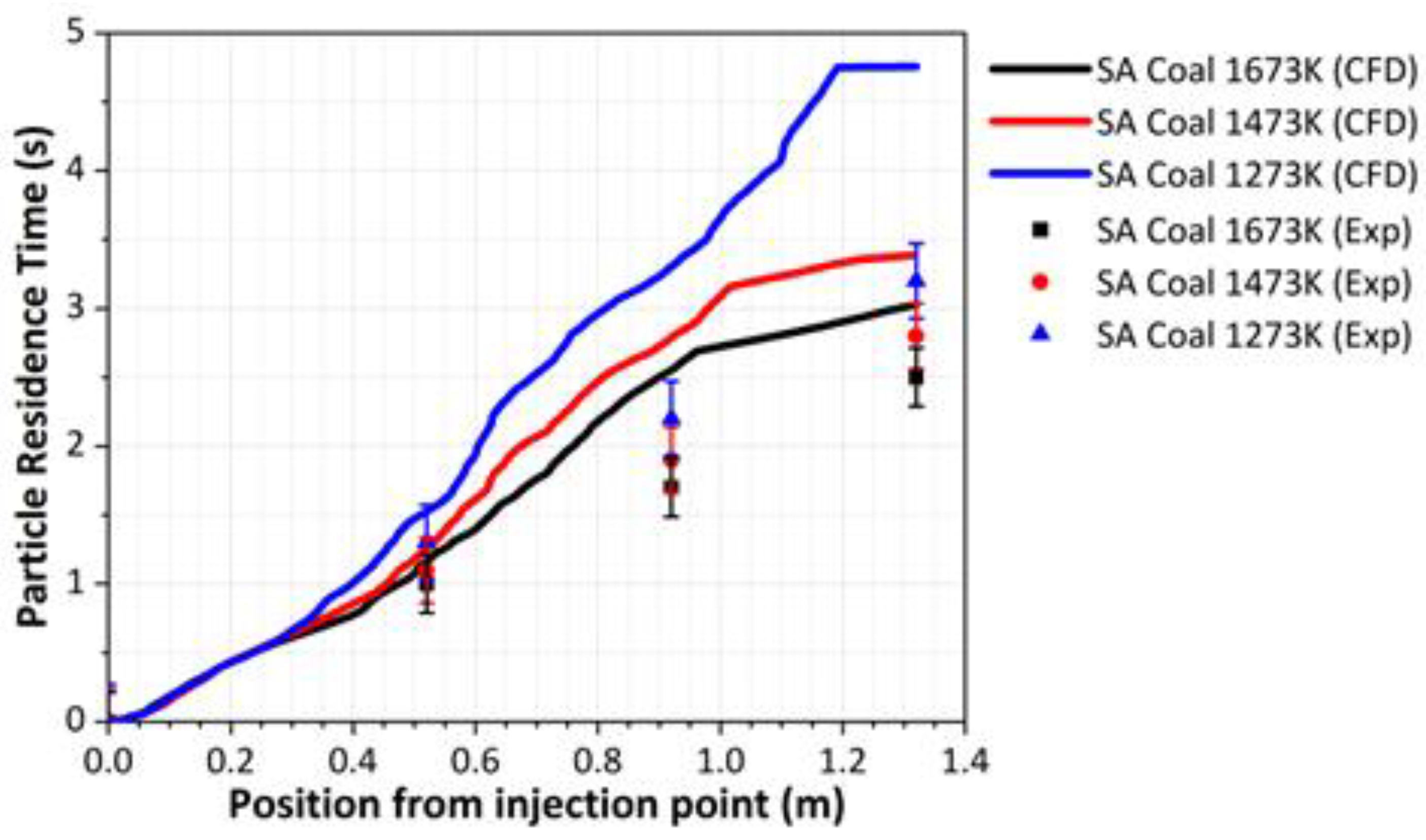
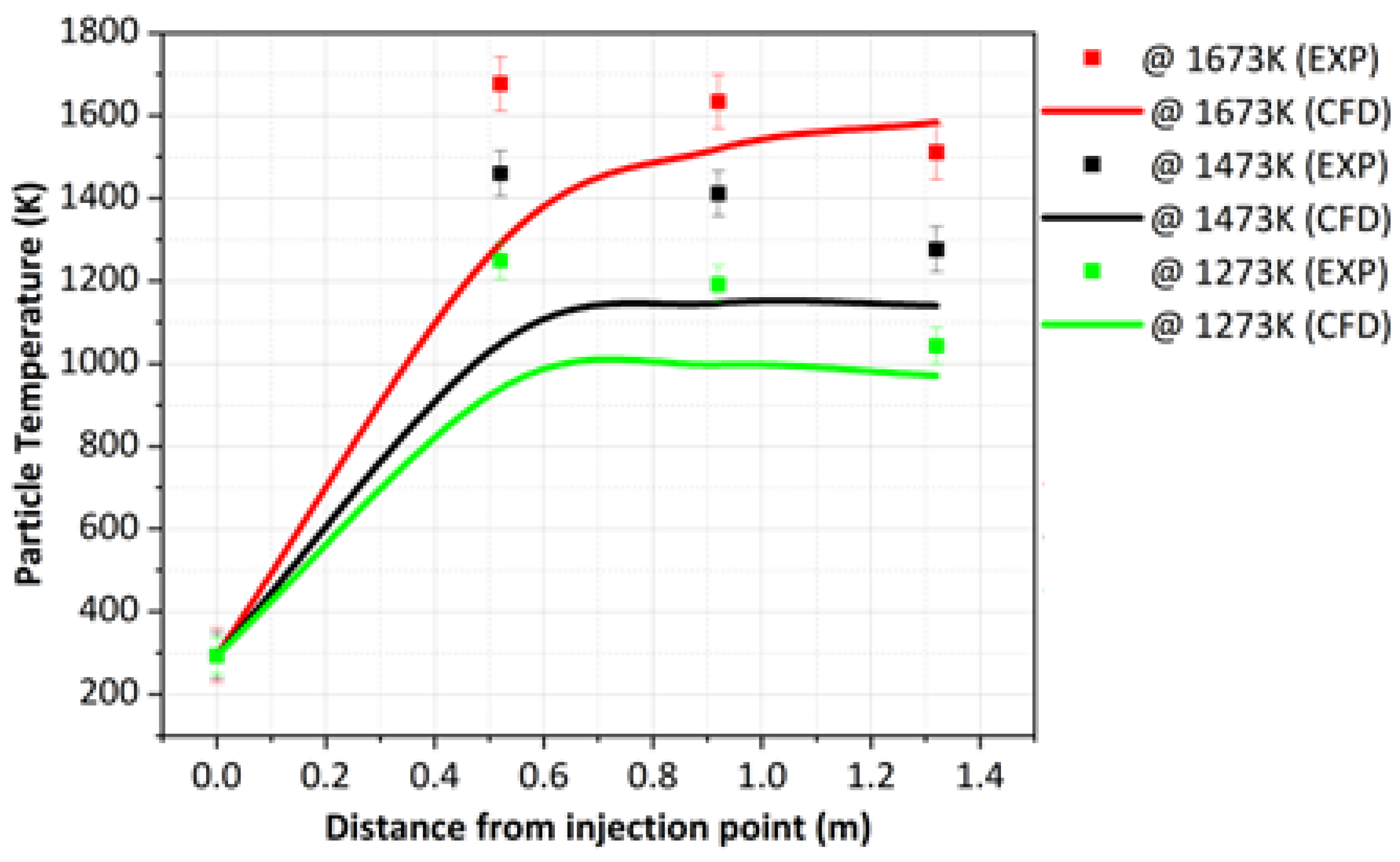
  • The variation in the particle residence time and temperature within the DTF was used to validate the cocombustion model. The predicted values produced a similar trend as compared to experimental values, though an overprediction was experienced with an average root mean square error (RMSE) of 1.117 at a 1273 K DTF wall temperature and 0.557 at a 1673 K DTF wall temperature. This overprediction was attributed to various factors related to the experimental procedure; hence, further research with regard to the characterisation of the char and volatiles produced by devolatilisation was suggested.
  • Increasing the Pinus sawdust blending ratio resulted in more volatiles being released, as mirrored by the proximate composition of the fuel blends. As such, the volatile composition on the fuel blends showed that the molar ratio of carbon increased with blending (0% to 30% sawdust) from 0.292 up to 0.579. The hydrogen and oxygen molar ratios also increased with Pinus sawdust blending, though to a lesser magnitude. The nitrogen molar ratio decreased from 0.086 to 0.052 as blending with Pinus sawdust increased, whilst the sulphur molar ratio decreased marginally.
  • The cocombustion model was able to bring synergy between various submodels of interest which tend to be overlooked in certain instances. The eddy dissipation concept submodel captured the combustion mechanisms successfully; the weighted sum of grey gases model captured the radiation from the combustion products successfully.
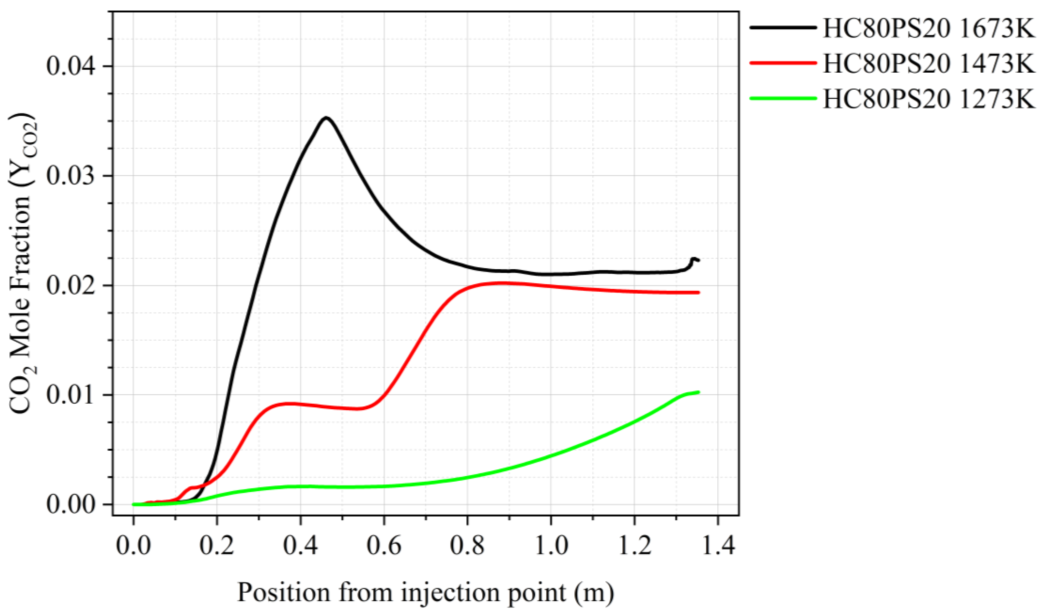
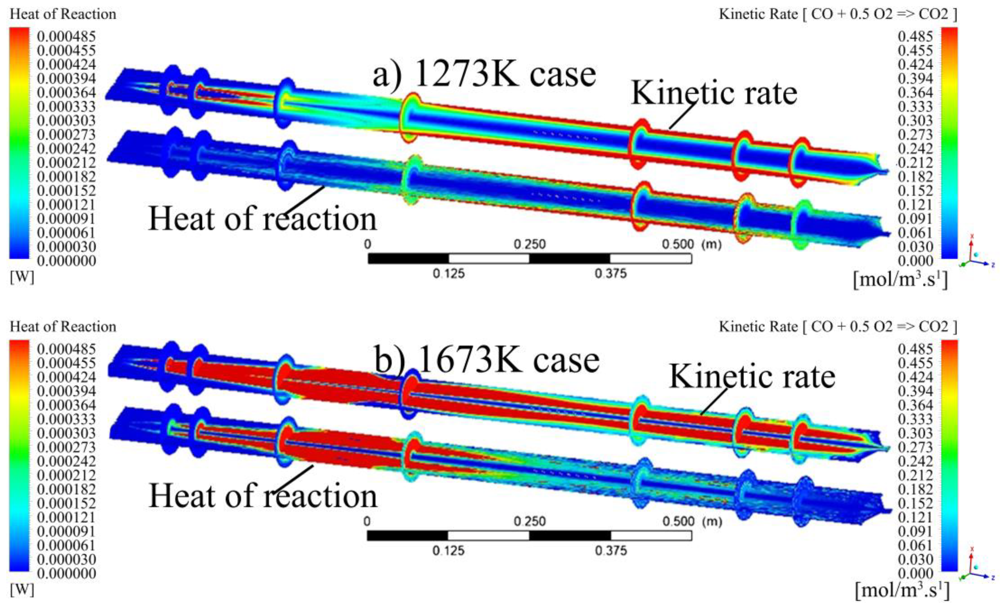
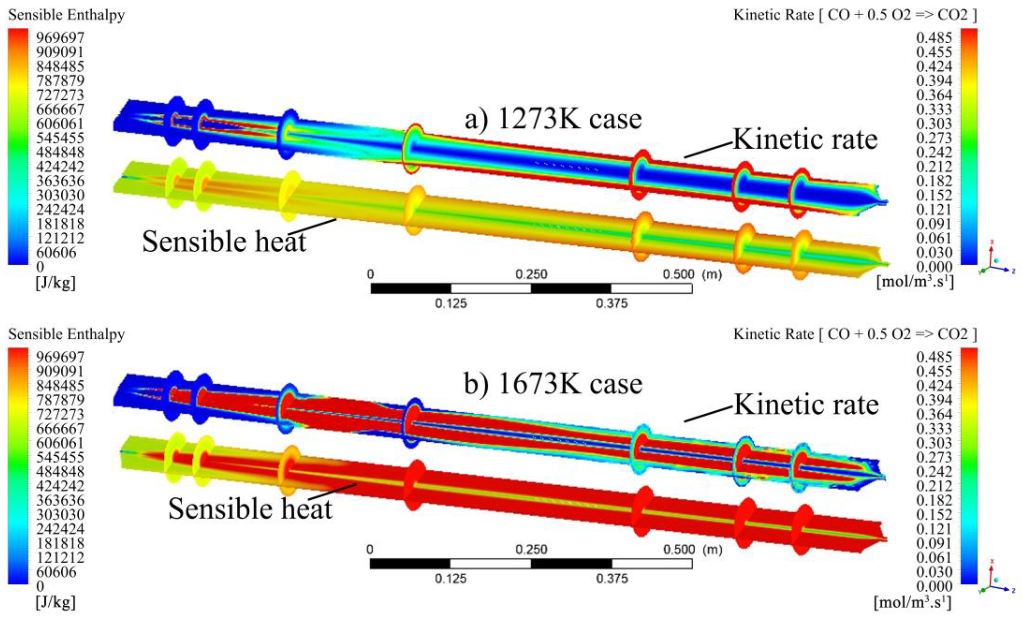
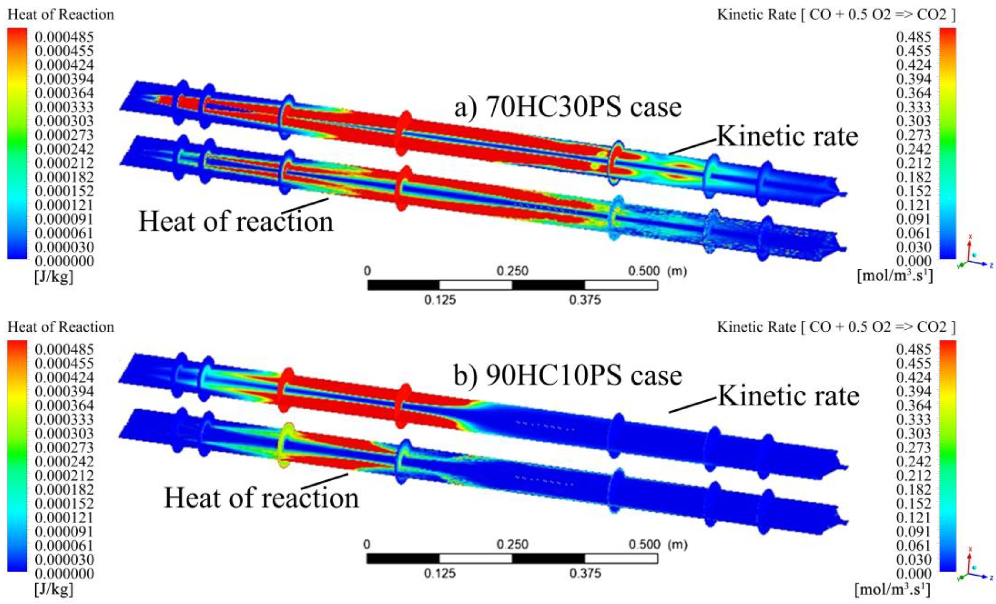
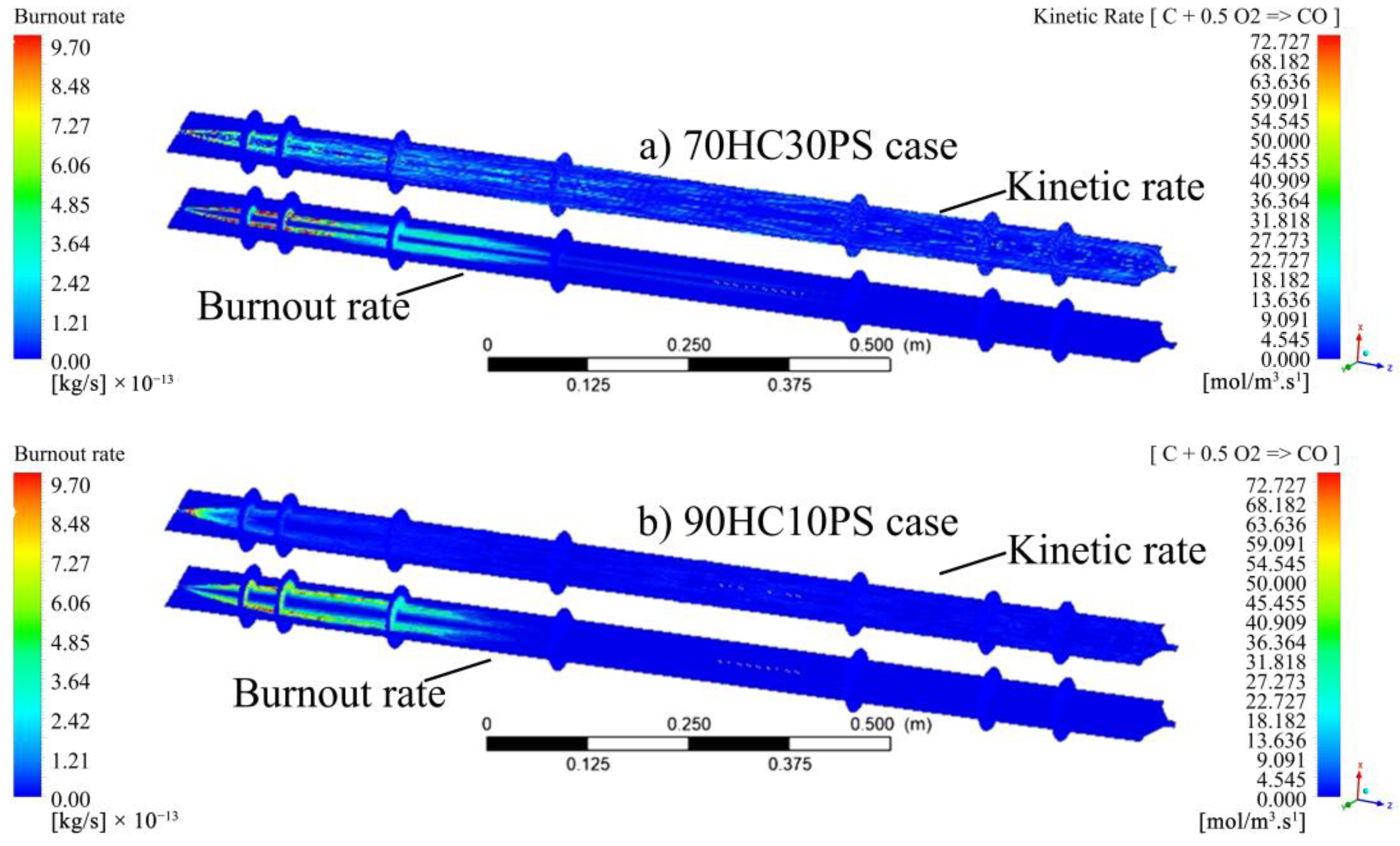
  • The visualisation of various profiles highlighted the co-dependency of certain combustion parameters on others. The discrete-phase particle burnout profiles were shown to be dependent on the oxidation of CO to form CO2 kinetic rate of reaction. It was also made evident that low DTF wall temperatures hindered the oxidation of CO to form CO2, thus delaying the reaction zone to an average location of 0.8 m from the injection point as compared to the initial 0.4 m obtained at high DTF wall temperatures.
  • Blending affected the heat of the reaction by promoting the onset of the reaction zone as well as increasing the combustion intensity within the reaction zone. The gradual release of heat was shown to be directly linked to the gradual burnout of the char particle. In conclusion, the reaction zone was modelled successfully to highlight the important combustion parameters.

Author Contributions

G.T.M. was responsible for conceptualisation, formal analysis, investigation, methodology, and writing of this manuscript. D.M.M. was responsible for funding acquisition and resources, as well as reviewing and editing of this manuscript. All authors have read and agreed to the published version of the manuscript.

Funding

This research received no external funding.

Data Availability Statement

The raw data supporting the conclusions of this article will be made available by the authors on request.

Acknowledgments

Special thanks to the University of Johannesburg, South Africa, for supporting the authors during their research.

Conflicts of Interest

The authors declare no conflicts of interest.

Nomenclature

The following units, symbols, and abbreviations were used in this manuscript:
Units
EaActivation energy (kJ/mol)
TStatic temperature (K)
APre-exponential factor (s−1)
UiVelocity (m/s)
Greek Symbols
ρDensity
φVariable (mass, specific enthalpy, or species mass fraction)
ΓVariable diffusion coefficient
Variable source or sink
Abbreviations
HCBituminous coal
PSPinus sawdust
TGAThermogravimetric analysis
CFDComputational fluid dynamics
FCFixed carbon
VMVolatile matter
DTFDrop tube furnace
EDCEddy dissipation concept
HHVHigher heat value
GCIGrid convergence index
Subscripts
dafDry ash free
volVolatile

References

  1. Zhou, C.; Gao, F.; Yu, Y.; Zhang, W.; Liu, G. Effects of Gaseous Agents on Trace Element Emission Behavior during Co-Combustion of Coal with Biomass. Energy Fuels 2020, 34, 3843–3849. [Google Scholar] [CrossRef]
  2. Benim, A.C.; Deniz Canal, C.; Boke, Y.E. Computational Investigation of Oxy-Combustion of Pulverized Coal and Biomass in a Swirl Burner. Energy 2022, 238, 121852. [Google Scholar] [CrossRef]
  3. Cardoso, J.S.; Silva, V.; Chavando, J.A.M.; Eusébio, D.; Hall, M.J. Numerical Modelling of the Coal Phase-out through Ammonia and Biomass Co-Firing in a Pilot-Scale Fluidized Bed Reactor. Fuel Commun. 2022, 10, 100055. [Google Scholar] [CrossRef]
  4. Wei, D.; An, D.; Wang, T.; Zhang, H.; Guo, Y.; Sun, B. Influence of Fuel Distribution on Co-Combustion of Sludge and Coal in a 660 MW Tangentially Fired Boiler. Appl. Therm. Eng. 2023, 227, 120344. [Google Scholar] [CrossRef]
  5. Lyu, Q.; Wang, R.; Du, Y.; Liu, Y. Numerical Study on Coal/Ammonia Co-Firing in a 600 MW Utility Boiler. Int. J. Hydrogen Energy 2023, 48, 17293–17310. [Google Scholar] [CrossRef]
  6. Marangwanda, G.T.; Madyira, D.M.; Ndungu, P.G.; Chihobo, C.H. Combustion Characterisation of Bituminous Coal and Pinus Sawdust Blends by Use of Thermo-Gravimetric Analysis. Energies 2021, 14, 7547. [Google Scholar] [CrossRef]
  7. Jin, W.; Si, F.; Kheirkhah, S.; Yu, C.; Li, H.; Wang, Y. Numerical Study on the Effects of Primary Air Ratio on Ultra-Low-Load Combustion Characteristics of a 1050 MW Coal-Fired Boiler Considering High-Temperature Corrosion. Appl. Therm. Eng. 2023, 221, 119811. [Google Scholar] [CrossRef]
  8. Gao, H.; Runstedtler, A.; Majeski, A.; Boisvert, P.; Campbell, D. Optimizing a Woodchip and Coal Co-Firing Retrofit for a Power Utility Boiler Using CFD. Biomass Bioenergy 2016, 88, 35–42. [Google Scholar] [CrossRef]
  9. Gu, T.; Ma, W.; Guo, Z.; Berning, T.; Yin, C. Stable and Clean Co-Combustion of Municipal Sewage Sludge with Solid Wastes in a Grate Boiler: A Modeling-Based Feasibility Study. Fuel 2022, 328, 125237. [Google Scholar] [CrossRef]
  10. Chen, B.; Liu, B.; Shi, Z. Combustion Characteristics and Combustion Kinetics of Dry Distillation Coal and Pine Tar. Int. J. Aerosp. Eng. 2020, 2020, 8888556. [Google Scholar] [CrossRef]
  11. Choi, C.R.; Kim, C.N. Numerical Investigation on the Flow, Combustion and NOx Emission Characteristics in a 500 MWe Tangentially Fired Pulverized-Coal Boiler. Fuel 2009, 88, 1720–1731. [Google Scholar] [CrossRef]
  12. Mohanna, H. Combustion of Pulverized Biomass: Impact of Fuel Preparation and Flow Conditions. Ph.D. Thesis, Normandie Université, Montpellier, France, 2021. [Google Scholar]
  13. Ma, W.; Zhou, H.; Zhang, J.; Zhang, K.; Liu, D.; Zhou, C.; Cen, K. Behavior of Slagging Deposits during Coal and Biomass Co-Combustion in a 300 KW Down-Fired Furnace. Energy Fuels 2018, 32, 4399–4409. [Google Scholar] [CrossRef]
  14. Fang, Y.; Qiao, L.; Wang, C.; Luo, X.; Xiong, T.; Tian, R.; Tang, Z.; Sun, H. Study on the Influence of the Activation Energy on the Simulation of Char Combustion. IOP Conf. Ser. Earth Environ. Sci. 2019, 300, 042062. [Google Scholar] [CrossRef]
  15. Xinjie, L.; Shihong, Z.; Xincheng, W.; Jinai, S.; Xiong, Z.; Xianhua, W.; Haiping, Y.; Hanping, C. Co-Combustion of Wheat Straw and Camphor Wood with Coal Slime: Thermal Behaviour, Kinetics, and Gaseous Pollutant Emission Characteristics. Energy 2021, 234, 121292. [Google Scholar] [CrossRef]
  16. Wang, G.; Guiberti, T.F.; Cardona, S.; Jimenez, C.A.; Roberts, W.L. Effects of Residence Time on the NOx Emissions of Premixed Ammonia-Methane-Air Swirling Flames at Elevated Pressure. Proc. Combust. Inst. 2022, 39, 4277–4288. [Google Scholar] [CrossRef]
  17. Sarroza, A.C.; Bennet, T.D.; Eastwick, C.; Liu, H. Characterising Pulverised Fuel Ignition in a Visual Drop Tube Furnace by Use of a High-Speed Imaging Technique. Fuel Process. Technol. 2017, 157, 1–11. [Google Scholar] [CrossRef]
  18. Yin, C.; Rosendahl, L.A.; Kær, S.K. Towards a Better Understanding of Biomass Suspension Co-Firing Impacts via Investigating a Coal Flame and a Biomass Flame in a Swirl-Stabilized Burner Flow Reactor under Same Conditions. Fuel Process. Technol. 2012, 98, 65–73. [Google Scholar] [CrossRef]
  19. Demirbaş, A. Biomass Co-Firing for Boilers Associated with Environmental Impacts. Energy Sources 2005, 27, 1385–1396. [Google Scholar] [CrossRef]
  20. Xia, Y.; Zhang, J.; Tang, C.; Pan, W. Research and Application of Online Monitoring of Coal and Biomass Co-Combustion and Biomass Combustion Characteristics Based on Combustion Flame. J. Energy Inst. 2023, 108, 101191. [Google Scholar] [CrossRef]
  21. Kuznetsov, V.A.; Minakov, A.V.; Bozheeva, D.M.; Dekterev, A.A. International Journal of Greenhouse Gas Control Oxy-Fuel Combustion of Pulverized Coal in an Industrial Boiler with a Tangentially Fired Furnace. Int. J. Greenh. Gas Control 2023, 124, 103861. [Google Scholar] [CrossRef]
  22. Marangwanda, G.T.; Madyira, D.M.; Chihobo, C.H. Determination of Cocombustion Kinetic Parameters for Bituminous Coal and Pinus Sawdust Blends. ACS Omega 2022, 7, 32108–32118. [Google Scholar] [CrossRef] [PubMed]
  23. ANSYS. ANSYS FLUENT User’s Guide; ANSYS: Canonsburg, PA, USA, 2021; pp. 1–170. [Google Scholar]
  24. Yin, C.; Rosendahl, L.A.; Condra, T.J.; Kær, S.K. Use of Numerical Modeling in Design for Co-Firing Biomass in Wall-Fired Burners. Chem. Eng. Sci. 2004, 59, 3281–3292. [Google Scholar] [CrossRef]
  25. Al-Abbas, A.H.; Naser, J. Effect of Chemical Reaction Mechanisms and NOx Modeling on Air-Fired and Oxy-Fuel Combustion of Lignite in a 100-KW Furnace. Energy Fuels 2012, 26, 3329–3348. [Google Scholar] [CrossRef]
  26. Marangwanda, G.T.; Madyira, D.M.; Babarinde, T.O. Coal Combustion Models: An Overview. J. Phys. Conf. Ser. 2019, 1378, 032070. [Google Scholar] [CrossRef]
  27. Maisyarah, A.; Shiun, J.; Nasir, F.; Hashim, H. Ultimate and Proximate Analysis of Malaysia Pineapple Biomass from MD2 Cultivar for Biofuel Application. Chem. Eng. Trans. 2018, 63, 127–132. [Google Scholar] [CrossRef]
  28. Marangwanda, G.T.; Madyira, D.M. Experimental Investigation on the Effect of Blending Bituminous Coal with Pinus Sawdust on Combustion Performance Parameters. Heliyon 2024, 10, e27287. [Google Scholar] [CrossRef]
  29. Zou, C.; Cai, L.; Wu, D.; Liu, Y.; Liu, S.; Zheng, C. Ignition Behaviors of Pulverized Coal Particles in O2/N2 and O2/H2O Mixtures in a Drop Tube Furnace Using Flame Monitoring Techniques. Proc. Combust. Inst. 2015, 35, 3629–3636. [Google Scholar] [CrossRef]
  30. Liu, M.; Han, B.; Bai, J.; Ru, J.; Wang, X.; Xing, L.; Li, H.; Lv, S.; Gao, A.; Wang, Y.; et al. Investigation on the Synergistic Effects and Thermokinetic Analyses during Co-Combustion of Corn Stalk and Polyethylene Plastic: Effect of Heating Rate and Placement Method. Fuel 2025, 385, 134032. [Google Scholar] [CrossRef]
  31. Czajka, K.M.; Modliński, N.; Kisiela-Czajka, A.M.; Naidoo, R.; Peta, S.; Nyangwa, B. Volatile Matter Release from Coal at Different Heating Rates –Experimental Study and Kinetic Modelling. J. Anal. Appl. Pyrolysis 2019, 139, 282–290. [Google Scholar] [CrossRef]
  32. Mularski, J.; Lue, L.; Li, J. Development of a Numerical Method for the Rapid Prediction of Ignition Performance of Biomass Particles. Fuel 2023, 348, 128520. [Google Scholar] [CrossRef]
  33. Versteeg, H.K.; Malalasekera, W. An Introduction to Computational Fluid Dynamics: The Finite Volume Method Approach; Prentice Hall: Hoboken, NJ, USA, 1996. [Google Scholar]
  34. de Souza-Santos, M.L. Solid Fuels Combustion and Gasification; CRC Press: Boca Raton, FL, USA, 2010; ISBN 9781420047509. [Google Scholar]
  35. Roache, P.J. Perspective: A Method for Uniform Reporting of Grid Refinement Studies. J. Fluids Eng. 1994, 116, 405–413. [Google Scholar] [CrossRef]
  36. Potgieter, M.S.W.; Bester, C.R.; Bhamjee, M. Experimental and CFD Investigation of a Hybrid Solar Air Heater. Sol. Energy 2020, 195, 413–428. [Google Scholar] [CrossRef]
  37. Haider, A.; Levenspiel, O. Drag Coefficient and Terminal Velocity of Spherical and Nonspherical Particles. Powder Technol. 1989, 58, 63–70. [Google Scholar] [CrossRef]
  38. Zhou, Z.; Chen, L.; Guo, L.; Qian, B.; Wang, Z.; Cen, K. Computational Modeling of Oxy-Coal Combustion with Intrinsic Heterogeneous Char Reaction Models. Fuel Process. Technol. 2017, 161, 169–181. [Google Scholar] [CrossRef]
  39. Graeser, P.; Schiemann, M. Investigations on the Emissivity of Burning Coal Char Particles: Influence of Particle Temperature and Composition of Reaction Atmosphere. Fuel 2020, 263, 116714. [Google Scholar] [CrossRef]
  40. Zhang, J.; Zheng, S.; Chen, C.; Wang, X.; ur Rahman, Z.; Tan, H. Kinetic Model Study on Biomass Pyrolysis and CFD Application by Using Pseudo-Bio-CPD Model. Fuel 2021, 293, 120266. [Google Scholar] [CrossRef]
  41. Mandø, M.; Rosendahl, L.A.; Yin, C.; Sørensen, H. Pulverized Straw Combustion in a Low-NOx Multifuel Burner: Modeling the Transition from Coal to Straw. Fuel 2010, 89, 3051–3062. [Google Scholar] [CrossRef]
  42. Turns, S. An Introduction to Combustion: Concepts and Applications, 2nd ed.; McGraw-Hill Series in Mechanical Engineering; McGraw-Hill: New York, NY, USA, 1996; ISBN 9780077418946. [Google Scholar]
  43. Tang, L.; Xiao, J.; Mao, Q.; Zhang, Z.; Yao, Z.; Zhu, X.; Ye, S.; Zhong, Q. Thermogravimetric Analysis of the Combustion Characteristics and Combustion Kinetics of Coals Subjected to Different Chemical Demineralization Processes. ACS Omega 2022, 7, 13998–14008. [Google Scholar] [CrossRef]
  44. Di Blasi, C. Modeling Chemical and Physical Processes of Wood and Biomass Pyrolysis. Prog. Energy Combust. Sci. 2008, 34, 47–90. [Google Scholar] [CrossRef]
  45. Sadhukhan, A.K.; Gupta, P.; Saha, R.K. Modeling and Experimental Investigations on the Pyrolysis of Large Coal Particles. Energy Fuels 2011, 25, 5573–5583. [Google Scholar] [CrossRef]
  46. Vyas, A.; Chellappa, T.; Goldfarb, J.L. Porosity Development and Reactivity Changes of Coal–Biomass Blends during Co-Pyrolysis at Various Temperatures. J. Anal. Appl. Pyrolysis 2017, 124, 79–88. [Google Scholar] [CrossRef]
Figure 1. DTF mesh showing inlets.
Energies 18 01322 g001
Figure 2. DTF mesh showing outlet.
Energies 18 01322 g002
Figure 3. Furnace wall temperature calibration.
Energies 18 01322 g003
Figure 4. Mesh sensitivity analysis.
Energies 18 01322 g004
Figure 5. DTF stage 2 plot of experimental and predicted residence times of SA coal fuel.
Energies 18 01322 g005
Figure 6. DTF stage 2 plot of experimental and predicted particle temperatures of SA coal sample.
Energies 18 01322 g006
Figure 7. DTF stage 2 particle temperature on axial and radial planes for (a) 100HC and (b) 70HC30PS fuel samples at 1473 K DTF wall temperature.
Energies 18 01322 g007
Figure 8. DTF stage 2 particle temperature against axial particle position for a 70HC30PS fuel sample at (a) 1273K and (b) 1673 K DTF wall temperatures.
Energies 18 01322 g008
Figure 9. DTF stage 2 axial variation in CO2 mole fraction for an 80HC20PS fuel sample at different DTF wall temperatures.
Energies 18 01322 g009
Figure 10. DTF stage 2 heat of reaction contours and kinetic reaction rate contours for a 70HC30PS fuel sample at (a) 1273 K and (b) 1673 K DTF wall temperatures.
Energies 18 01322 g010
Figure 11. DTF stage 2 particle burnout contours and kinetic reaction rate contours for a 70HC30PS fuel sample at (a) 1273 K and (b) 1673 K DTF wall temperatures.
Energies 18 01322 g011
Figure 12. DTF stage 2 sensible heat contours and kinetic reaction rate contours for a 70HC30PS fuel sample at (a) 1273 K and (b) 1673 K DTF wall temperatures.
Energies 18 01322 g012
Figure 13. DTF stage 2 heat of reaction contours and kinetic reaction rate contours for (a) 70HC30PS and (b) 90HC30PS at 1473 K.
Energies 18 01322 g013
Figure 14. DTF stage 2 DPM burnout contours and kinetic reaction rate contours for (a) 70HC30PS and (b) 90HC10PS at 1473 K.
Energies 18 01322 g014
Table 1. Summary of methods used to report on combustion parameters.
DescriptionFuelsMethod of Reporting on
IgnitionBurnoutIntensityStability
Combustion in a 150 kW reactor [18]Coal and wheat strawTemperaturesChar
percentage
--
Lab-scale bubbling fluidised bed combustor [19]Coal, lignite, spruce wood, wheat straw, and hazelnut shell-Unburnt carbon--
Cocombustion in a 660 MW tangentially fired boiler [4]Coal and sewage sludge--Heat flux-
Experimental study on combustion with nitrogen [20]Coal, poplar wood, and corn stalksTemperature
Radiation spectrum
--Image
processing
Cocombustion in a 500 MW boiler [21]Coal slurryTemperatureSpecies molar fractions--
Table 2. Volatile composition determination.
Constituent%Weight%Mol
C C daf FC daf VM daf 1 12 × C daf FC daf VM daf × Mr volatile = a
H H daf VM daf 1 1 × H daf VM daf × Mr volatile = b
O O daf VM daf 1 16 × O daf VM daf × Mr volatile = c
N N daf VM daf 1 14 × N daf VM daf × Mr volatile = d
S S daf VM daf 1 32 × S daf VM daf × Mr volatile = e
Table 3. Chemical compositions of fuel blends.
Fuel BlendProximate Analysis
on a Dry Basis
Volatile Molar
Composition
Volatile Molar MassEnthalpy of Formation
for Volatile (Hf,vol)
100HC53.97FC, 23.10VM, 22.93AshC0.292H2.200O0.618N0.086S0.01417.24−5.904 × 10⁷
90HC10PS48.21FC, 29.91VM, 21.88AshC0.535H2.102O0.556N0.0646S0.011118.68−7.862 × 10⁷
80HC20PS46.35FC, 31.82VM, 21.83AshC0.559H2.36O0.618N0.0585S0.01120.11−9.819 × 10⁷
70HC30PS46,02FC, 33.74VM, 20.24AshC0.579H2.615O0.683N0.052S0.01121.55−1.178 × 10⁸
100PS15.62FC, 80.68VM, 3.70AshC1.107H2.37O0.99N0.0131.63−2.548 × 10⁸
Table 4. Activation energy and pre-exponential factor values for the fuel blends heated in air.
Fuel BlendStageEa (kJ/mol)A (s−1)
100HC Volatile combustion92.985.84 × 105
Char combustion52.901.16 × 103
90HC10PS Volatile combustion107.895.05 × 106
Char combustion68.992.78 × 104
80HC20PSVolatile combustion104.952.94 × 108
Char combustion90.529.53 × 105
70HC30PSVolatile combustion106.052.72 × 109
Char combustion103.856.12 × 107
Table 5. Combustion model boundary conditions.
PhysicsModel
TurbulenceRNG k-epsilon, scalable wall function
Radiation Discrete ordinate model, P1 model weighted sum of grey gases model (WSGGM)
Particle distribution40 continuous-phase iterations per DPM iteration
Rosin–Rammler diameter distribution
InletsFuel velocity inlet as 1.85 m/s
For a 30° modelled section, total fuel mass flow rate translated to 2.08 × 10⁻⁶ kg/s, primary carrier gas mass flow rate was 4.85 × 10⁻⁷ kg/s, and secondary carrier gas was 2.43 × 10⁻⁵ kg/s
Chemical rectionSpecies transport option, eddy dissipation concept
Table 6. South African coal chemical analysis.
AshVMFCMCCHNSCarbonatesOHHV (MJ/kg)
28.920.447.92.854.752.411.301.473.964.4121.00
Table 8. DTF stage 2 experimental and predicted residence times of SA coal sample.
PositionDesignationResidence Time at Various Furnace Wall Temperatures (s)
1273 K1473 K1673 K
520 mmSA coal (Exp)1.30001.10001.0000
SA coal (CFD)1.52171.27551.0826
920 mmSA coal (Exp)2.20001.90001.7000
SA coal (CFD)3.32902.95572.5335
1320 mmSA coal (Exp)3.20002.80002.5000
SA coal (CFD)4.75513.30352.9774
RSME1.11680.68280.5566
Table 9. DTF stage 2 experimental and predicted particle temperatures of SA coal sample.
PositionDesignationParticle Temperature (K)
1273 K1473 K1673 K
520 mmSA coal (Exp)1248.001459.821676.80
SA coal (CFD)939.611048.271289.18
920 mmSA coal (Exp)1191.801411.481633.88
SA coal (CFD)997.211145.571519.20
1320 mmSA coal (Exp)1042.741276.331511.19
SA coal (CFD)970.601140.551583.59
RSME0.17590.20520.1422
Disclaimer/Publisher’s Note: The statements, opinions and data contained in all publications are solely those of the individual author(s) and contributor(s) and not of MDPI and/or the editor(s). MDPI and/or the editor(s) disclaim responsibility for any injury to people or property resulting from any ideas, methods, instructions or products referred to in the content.

