A Comparative Analysis of Machine Learning Algorithms in Energy Poverty Prediction

Abstract

Given the limited potential of conventional statistical models, machine learning (ML) techniques in the field of energy poverty have attracted growing interest, especially during the last five years. The present paper adds new insights to the existing literature by exploring the capacity of ML algorithms to successfully predict energy poverty, as defined by different indicators, for the case of the “Urban Region of Athens” in Greece. More specifically, five energy poverty indicators were predicted on the basis of socio-economic/technical variables through training different machine learning classifiers. The analysis showed that almost all classifiers managed to successfully predict three out of five energy poverty indicators with a remarkably good level of accuracy, i.e., 81–94% correct predictions of energy-poor households for the best models and an overall accuracy rate of over 94%. The most successful classifier in terms of energy poverty prediction proved to be the “Random Forest” classifier, closely followed by “Trees J48” and “Multilayer Perceptron” classifiers (decision tree and neural network approaches). The impressively high accuracy scores of the models confirmed that ML is a promising tool towards understanding energy poverty drivers and shaping appropriate energy policies.

1. Introduction

1.1. The Problem of Energy Poverty

Research on energy poverty is gaining more and more interest over the last years, with numerous new enquiries on the definition, measurement, and analysis of the phenomenon. In general, energy poverty is a serious socio-economic problem, with different conceptual approaches throughout the world. In the developed world, it is connected to the lack of access to clean energy services and electricity for 2 billion people and 750 million people, respectively [1], whereas, in the developed world, it is mainly associated with the inability of households to adequately meet their energy needs at an affordable cost.

A policy and academic acknowledgement of the issue has been developed recently, arguing that energy poverty is rather a social than an inherently economic or environmental issue, following global issues [2]. Indeed, vulnerable consumers were inevitably affected by the negative impact of the COVID-19 pandemic outbreak on the energy market [3,4]. The increase in energy prices along with the pandemic led crowds of people to difficulty or inability to pay their energy bills [5]. Hence, final energy use was drastically reduced by the household sector, primarily among vulnerable parts of the population, such as low-income households [6]. This issue has intensified in Europe throughout the last years, as a consequence of financial crises and global geopolitical crises (e.g., war in Ukraine, conflicts in the Middle East), which have brought about great instability and great increases in energy prices.

Greece is among the European countries with severe energy poverty issues [7], also coming 5th in ranking with people “at risk of poverty or social exclusion” (26.1% of the country’s population) [8]. Over the past decade, a significant rise in fuel costs has taken place, combined with a remarkable decrease in the real value of households’ disposable incomes. At the same time, a dramatic rise in the level of food prices has been recorded, and environmental and health issues have multiplied due to the use of inappropriate and low-cost or free materials as fuels for space heating.

Research on energy poverty in Greece has gained increasing attention over the last decade, mainly due to the deterioration of the problem recently. Indicatively, Atsalis et al. [9] analyzed energy poverty as being expressed by the 10% indicator (ratio of energy expenses to the household’s income), based on data from the Household Budget Survey of the Hellenic Statistical Authority, showing an energy poverty rate of about 20–25% in Greece in 2013. Papada and Kaliampakos [10] carried out a primary survey in the whole country, revealing that 58% of households in Greece faced energy poverty in 2015, according to the 10% indicator, while a similar study in the mountainous areas of the country pointed out the intensity of the problem in these areas, affecting 73.5% of mountainous households [11]. Further works have studied the problem in specific geographical areas, such as in Athens [12,13], in the Attica region [14], in Western and Central Macedonia [15], in the Thessaloniki Urban Complex [16], etc. Moreover, new indicators have been suggested over time, such as, for instance, the indicator of “Degree of Coverage of Energy Needs” [17], demonstrating that 46% of Greek households compress their energy needs.

Numerous works have used traditional statistical tools to measure energy poverty in Greece. Indicatively, logistic regression models were used by Lyra et al. [18], showing that 40% of households in Greece face energy poverty, while also highlighting certain variables, i.e., household income, dwelling type, location of residence, and educational level, as decisive predictors of the problem. Similarly, binary logistic regression models were used by Kalfountzou et al. [19] to predict various indicators (10%, 2M, M/2) based on certain socio-economic variables. Halkos and Kostakis [20] employed a probit model [15], according to which 9–10% of Greek households are steadily vulnerable to energy poverty, and factors such as income level, educational level, housing characteristics, migration background, and employment proved to be the ones that mostly affect the problem.

However, given the limited potential of conventional statistical models [21] and the identification that current challenges entail large and complex datasets, there is a growing need for models with improved predictive power [22], a finding that has been especially confirmed, among other research areas, for the field of energy poverty mitigation [23]. In this context, machine learning algorithms predicting energy poverty have started attracting increasing attention recently.

1.2. Machine Learning and Energy Poverty

Although conventional regression models can be used to explore relationships between socio-economic variables and energy poverty risk, the employment of machine learning (ML) offers three (3) distinct advantages for such types of analyses:

• Modern-day issues often include large amounts of data with multiple features, which are challenging for traditional regression models to handle. ML algorithms though are fundamentally designed to process and analyze large and complex datasets effectively.
• Conventional regression models typically require prior assumptions regarding the correlations between the factors, potentially inserting bias in the analysis or limiting its scope. ML algorithms though learn from real data and identify correlations through the training process, without requiring any prior assumptions.
• ML algorithms are inherently able to address non-linear dependencies, which is a main requirement for studying and analyzing complex phenomena such as energy poverty, whereas traditional regression models are better suited to address linear relationships.

The literature shows that a large number of works have used machine learning techniques to study partial aspects of energy poverty, including high energy prices, low household income, and low energy efficiency of residences [24], but a limited quantity of such works focus on energy poverty as a multidimensional phenomenon [24]. Actually, machine learning techniques addressing energy poverty alleviation have begun to gain popularity, mainly during the last five years, with the most famous among them being decision tree-based and neural network-based approaches [24].

As regards decision tree-based approaches, Longa et al. [25] used the XGBoost classifier to predict energy poverty, defined by the ratio of household energy costs to household income (four risk categories) in the Netherlands, using as input variables income and socio-economic factors (household size, economic value of the property, property status, house age, and average population density). Al Kez et al. [26] used a random forest classifier to predict energy poverty, defined by the “Low Income Low Energy Efficiency” indicator (four risk categories) in the UK, based on socio-economic data and satellite remote sensing, using secondary statistical data (UK English Housing Survey). A random forest classifier was also used by Spandagos et al. [27] to predict energy poverty for all the EU-28 countries, based on data from Eurostat’s EU-SILC survey. van Hove et al. [28] trained a gradient boosting classifier (CatBoost model) in order to identify energy poverty risk (four risk categories), based on socio-economic factors and using data from a primary survey within 11 European countries. The same algorithm (CatBoost) was also used by Mukalabai et al. [29] in order to explore energy poverty in the global south (South America, Africa, and Asia).

As regards neural network-based approaches, Pino-Mejías et al. [30] used artificial neural networks (ANNs) to predict the “Fuel Poverty Potential Risk Index” in Chile and, particularly, in the Bio-Bio Region. Building upon this work, Bienvenido-Huertas et al. [31] applied ANNs to predict the same indicator (FPPRI) in Chile’s three cities with different climate zones (Valparaiso, Concepción, and Santiago). Papada and Kaliampakos [32] used a multilayer perceptron classifier to predict energy poverty defined by various “objective” indicators, using as inputs “subjective” indicators. In the developing world, Abbas et al. [33] employed a multilayer perceptron to predict the “Multidimensional Energy Poverty Index” in Africa and Asia, using as input variables socio-economic variables of survey data.

Apart from studies using a distinct ML algorithm, there are numerous references employing two or more ML algorithms in terms of energy poverty prediction. Indicatively, Bienvenido-Huertas et al. [31] employed three ML algorithms, i.e., random forest, multilayer perceptron (ANN), and M5P, to predict the “2M” indicator of energy poverty in Spain. Hong and Park [22] applied different ML algorithms, i.e., ANN, decision tree, random forest, bagging, support vector machine, and extreme gradient boosting, to predict energy poverty based on secondary statistical data, with the random forest algorithm presenting the best performance among the predictive models. Three ML algorithms were employed by Gawusu et al. [34], including XGBoost—multiple linear regression (MLR), XGBoost—random forest (RF), and XGBoost—artificial neural network (ANN), to predict the “Multidimensional energy poverty index” in Wa, located in Ghana, concluding that the XGBoost—random forest (RF) algorithm achieved the best accuracy. Different ML algorithms were also applied by Balkissoon et al. [35], namely, decision tree, random forest, support vector machine, and extreme gradient boosting, to forecast energy poverty in Missouri, with the extreme gradient boosting showing the best performance among all the models. Grzybowska et al. [36] applied logistic regression, along with three ML algorithms, i.e., CatBoost, extreme gradient boosting, and balanced random forest, to forecast energy poverty—as being defined by the “inability to keep the home warm” indicator—in the Visegrad Group countries (Hungary, Slovakia, and Poland), based on data from Eurostat’s EU-SILC survey.

As a result, there is a growing number of studies adopting ML techniques to forecast energy poverty in the last five years. In an attempt to enhance the existing knowledge of ML performance in the field, in the present paper, different ML algorithms were employed to predict energy poverty depending on various socio-economic/technical variables within the “Urban Region of Athens” (URA) in Greece. More precisely, the Urban Region of Athens (URA) is the heart of Greater Athens, the capital of Greece, and the most densely populated area of the country. It covers a space of 412 km² and has a population of more than 3 million people (30% of the country’s population), making it the biggest urban area in Greece. Furthermore, apart from large parts of the population, the study area concentrates most services and facilities; hence, it is a research area of particular importance.

The rest of the paper is structured as follows: Section 2 introduces the methodology employed to conduct the survey. It presents the energy poverty indicators, as well as the predictors used. Additionally, this section describes the various ML algorithms and provides a description of how the accuracy of the models was evaluated. Section 3 provides the results of the research and discusses how they can be interpreted with respect to previous studies. Section 4 presents the main conclusions of the research.

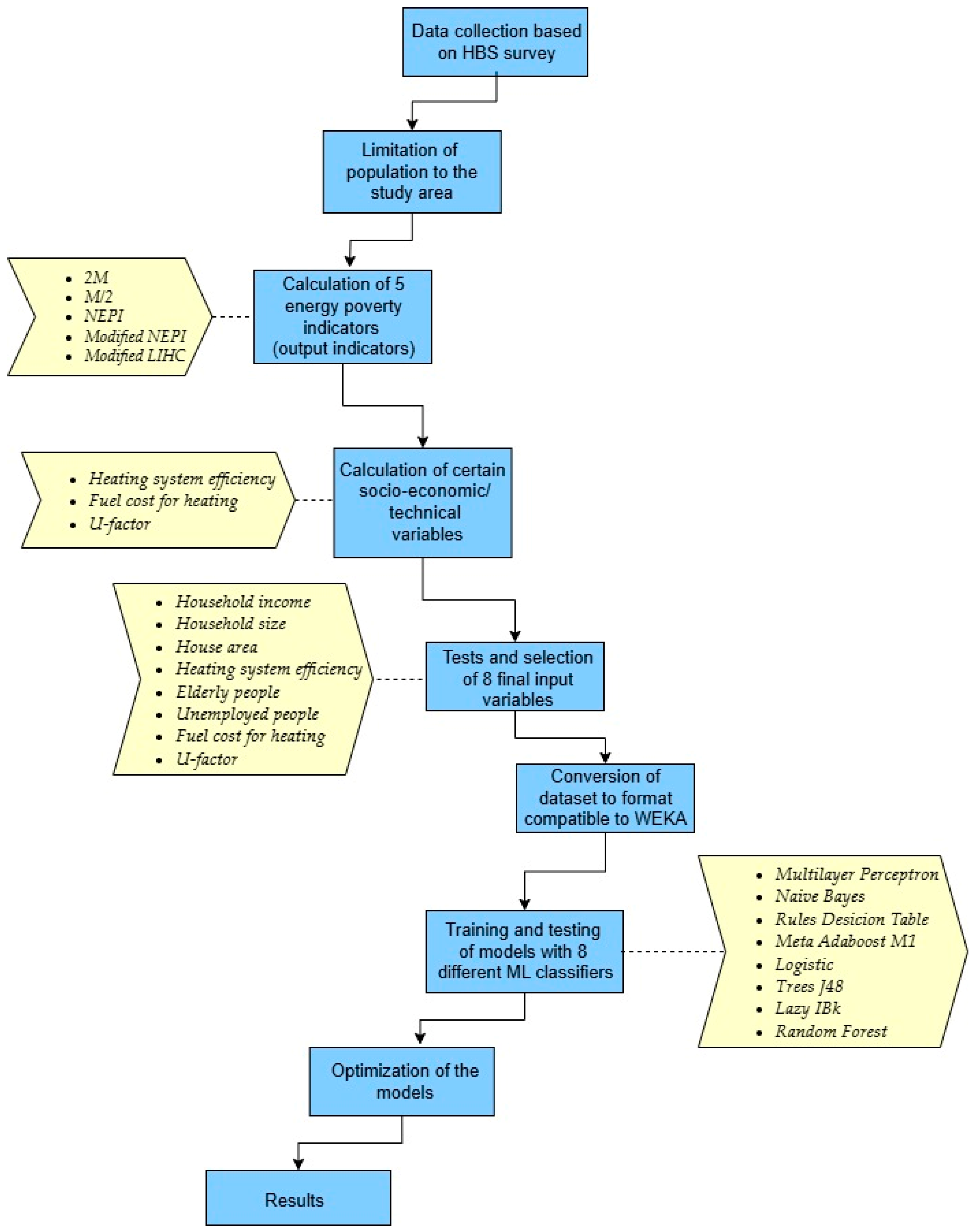
2. Materials and Methods

Data on energy poverty were collected using the Household Budget Survey (HBS) datasets that were obtained by the Hellenic Statistical Authority. The HBS survey microdata—provided at the household level—were obtained for the period 2017–2021. From the whole dataset and, in order to limit the sample to the Urban Region of Athens (URA), only observations related to the region “EL30–Attiki” (variable HA08) and to densely populated areas (variable HA09) were taken into account, amounting to 6645 observations.

The analysis aimed to predict energy poverty, as defined by different indicators (output indicators), on the basis of particular socio-economic/technical factors (input variables), using machine learning. In more detail, the authors identified five (5) energy poverty indicators as the most representative of the energy poverty problem, as they capture its crucial aspects (low income and high energy cost) from many different sides. The five (5) energy poverty indicators (output indicators) were calculated as described below:

• The 2M indicator classifies households as energy poor if their ratio of equivalised energy expenses to equivalised disposable income exceeds twice the national median ratio. Both the variables of energy expenses and income were equivalised in order to take into account differences in size and composition of the household, i.e., energy cost was divided by the equivalisation factors and disposable income by the equivalent household size based on the scale of equivalence of the modified OECD, accordingly.
• The M/2 indicator classifies households as energy poor if their absolute equivalised energy expenses are less than half the national median value.
• The official national energy poverty indicator (NEPI) classifies households as energy poor if (i) the annual expenditure on the total final energy consumed in the dwelling is less than 80% of the theoretically required amount of energy and (ii) the equivalised total household income is less than 60% of the median equivalised national income, based on the respective poverty definition in Greece.
• The modified NEPI indicator differs from the NEPI index only in point (i), by setting a different limit for classifying a household as energy poor, i.e., the limit of 60% vs. 80% used in the NEPI indicator [13]. In more detail, the share of 60% of the theoretical energy consumption, needed to guarantee an adequate level of energy services at home, represents the actual energy consumption of Greek households according to Greek circumstances.
• The modified LIHC (low income high cost) classifies households as energy poor if they have an equivalised residual income below 60% of the equivalised median national income. In order to calculate the equivalised residual income, 60% of equivalised required energy costs was deducted from the equivalised total income of the household. Then, this value was compared to 60% of the equivalised median national income, and if it was lower, the household was regarded as energy poor. Energy costs were equivalised according to the equivalisation factors employed in the official LIHC index.

The eight (8) socio-economic/technical factors used as main predictors of energy poverty are described below:

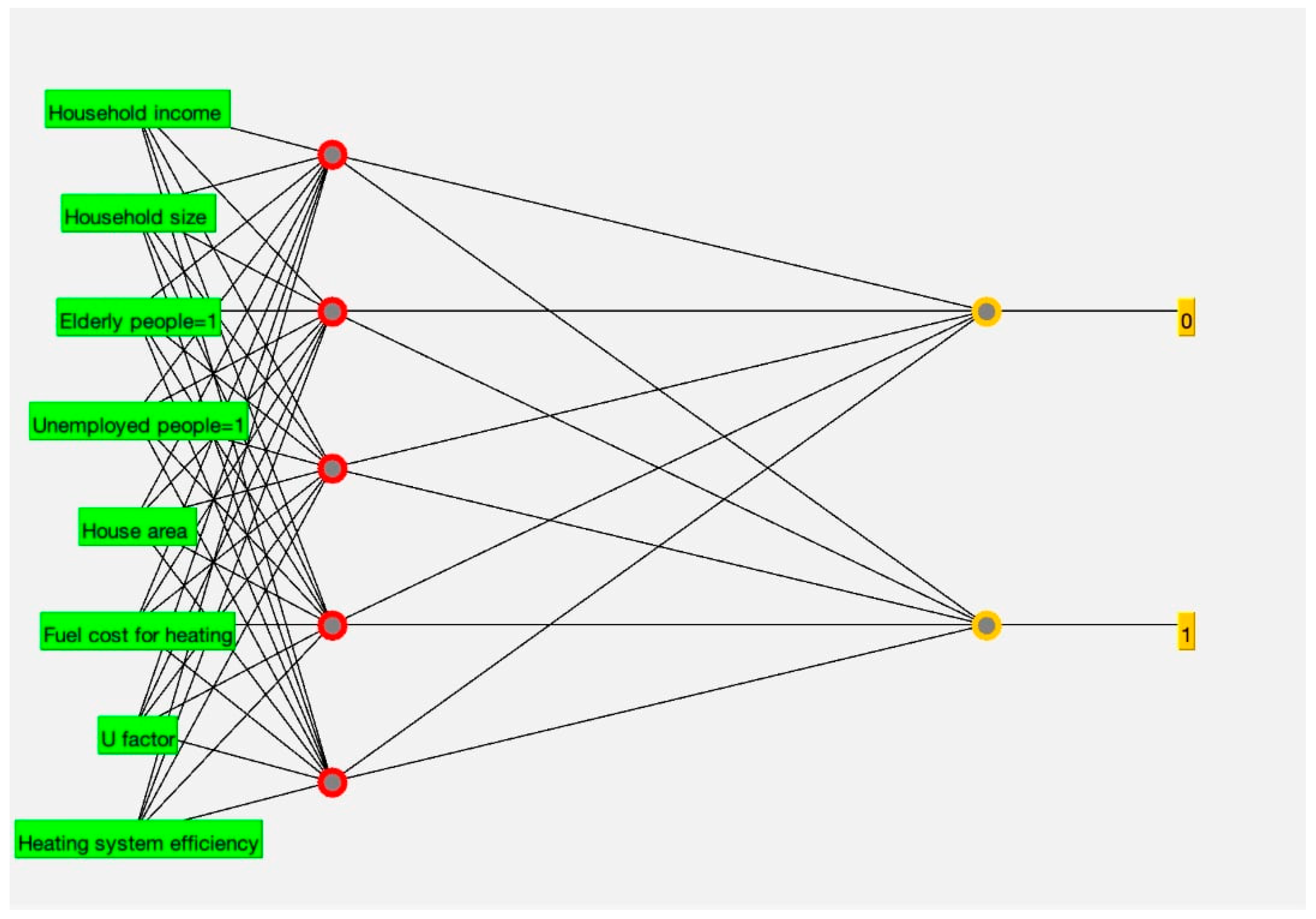
• Household income (HH099): continuous variable in HBS that represents net income, i.e., total income of all sources including non-monetary elements, before income taxes.
• Household size (HB05): integer variable in HBS that represents the number of household members.
• House area (DS017): continuous variable in HBS representing the square meters (m²) of the area of the residence.
• Heating system efficiency: continuous variable expressed in percentage. Estimates were made by the authors based on typical efficiency ratio values of heating systems in buildings.
• Elderly people: binary variable that indicates the presence of elderly people in households (1 if people over 65 years old live in the residence and 0 otherwise).
• Unemployed people: binary variable that indicates the presence of unemployed people in households (1 if unemployed people live in the residence and 0 otherwise).
• Fuel cost for heating: continuous variable that is expressed in EUR/kWh. Estimates were made by the authors based on statistics from the “Liquid Fuel Prices Observatory” of the Ministry of Development [37], as well as from other sources [38].
• U-factor: building continuous technical variable that is expressed in W/m² K. Estimates were made by the authors based on the proposed coefficients from the “Regulation of Energy Efficiency in Buildings” in Greece [39].

The final selection of the predictors (input variables) was based on numerous tests that examined several different variables to identify the most decisive factors affecting energy poverty. The predictors that gave the best results in the tested models were finally selected.

After the calculation of indicators and variables, the data selected were modified, i.e., missing values were detected, the file was converted to an “arff” file, etc., in order to be transferred in the appropriate format to “WEKA”, i.e., the application used to train machine learning algorithms. More precisely, written in Java at the University of New Zealand, WEKA (Waikato Environment for Knowledge Analysis) provides several machine learning algorithms and a set of data preprocessing tools [40]. The classifiers included in WEKA are generally divided into six (6) main categories, i.e., functions, decision trees, Bayesian classifiers, rules, meta-learning algorithms, and lazy classifiers.

• From the group of functions’ classifiers, multi-layer perceptron (MLP) and logistic regression were selected for the present analysis. More specifically:
  • The multilayer perceptron is a kind of artificial neural network, which uses a nonlinear activation function within its hidden layer, providing a nonlinear mapping between the input and the output layer. Its basic structure is divided into three layers, of which one layer defines the input values, another one or more the mathematical function, and, finally, the output layer that captures the final result. A large number of neurons in each layer are linked with weighted connections, in which entire layers of neurons are interlinked through weighted connections with every neuron [41].
  • Logistic regression is a type of classification algorithm that is used under supervised learning and determines the likelihood of an event, with a binary output. In contrast with linear regression, which returns a continuous output, logistic regression returns a probability score of the outcome of the binary event. A logistic regression model identifies all the underlying “weights” and “biases” based on the provided dataset during training and understands how to correctly classify the dataset using the dependent categorical variables.
• From the group of decision trees’ classifiers, the J48 classification algorithm and Random Forest were selected for the present analysis. In general, a decision tree builds a tree that utilizes the branching technique to show every possible outcome of a decision. Each internal node in its decision tree representation symbolizes a feature, every branch symbolizes the result of the parent node, and, finally, each leaf symbolizes the class label. In order to classify a case, a top-down “divide and conquer” strategy begins at the root of the tree [42]. More specifically:
  • The J48 classification algorithm is based on the C4.5 algorithm, an extension of Ross Quinlan’s ID3, i.e., a statistical decision tree classifier. J48 is extremely useful for examining categorical and continuous data. In WEKA, J48 includes many additional features that can be configured by the user, such as decision tree pruning, missing value estimation, and attribute value range. Pruning, for instance, is the act of selecting the largest tree and removing all the branches below this level. It is an essential process that handles the phenomenon of overfitting [43].
  • Random forest classification algorithm is based on forming multiple individual decision trees that are derived from a different sample taken from the dataset. At every tree node, a random subgroup is utilized in order to split the dataset into increasingly uniform subgroups. The subgroup of variables achieving the best performance in terms of data purity is chosen at this tree node. After creating the forest of decision trees, the ultimate outcome of classification is based on voting by every tree. The most votes give the final classification [44].
• From the group of Bayesian classifiers, naïve Bayes was selected for the present analysis. Bayes’ theorem with independent hypotheses among the predictors is the basic concept of the naïve Bayes classifier. The simplest approach to the Bayes network in WEKA is the naïve Bayes, in which all attributes of a dataset, given the target class, are independent of each other. Thus, in naïve Bayes’ network, the class has no “parent”, i.e., it does not receive its properties from another dataset, and each attribute has the class as a unique “parent” [45]. The classification model is created without complex iterative parameter estimation. Due to this feature, Bayesian classifiers are useful even for very large datasets and provide reliable results for complex, real-world problems [41].
• From the group of rules’ classifiers, Decision Table was selected for the present analysis. This algorithm constructs a classifier represented in the form of a decision table and represents a particularly simple classifier regarding its classification methodology. It evaluates subsets of features using a sequential search for the optimal initial choice and is able to use cross-validation for the evaluation procedures. Basically, through the decision table, a comprehensive system is created that includes all possible scenarios of conditions under which classification can be performed, from which the algorithm determines the scenario that presents the highest accuracy and probability of occurrence [46].
• From the group of meta-learning algorithms, AdaBoost.M1 was selected for the present analysis. Meta-learning algorithms transform classification algorithms into more powerful classification tools, significantly improving their learning capabilities. This improvement is achieved by different methods, such as by combining different output data from separate classifiers. WEKA includes numerous meta-learning algorithms, which follow different forms of algorithm improvement. The main ones are boosting, bagging, and randomization, combining classifiers and cost-sensitive learning. From the available improvement algorithms, a boosting-type algorithm was selected. Boosting is a general improvement method that creates a strong classifier from a number of weak classifiers. This is carried out by creating a model from the training data and then creating a second model that tries to correct the errors of the first model. Models are added until the training set is optimally predicted or until a maximum number of models are added. A classic case of a boosting algorithm is AdaBoost.M1 (or AdaBoost). AdaBoost.M1 can be used to boost the performance of any machine learning algorithm, but it works most efficiently on algorithms with low training capacity. Thus, AdaBoost delivers maximum performance when used to boost decision trees [47].
• From the group of lazy classifiers, IBk (instance-based learning with parameter k) was selected for the present analysis. The principle of an IBk algorithm is essentially equivalent to the kNN (k-nearest neighbor) algorithm, using the same distance metric. When classifying with kNN, the value is classified according to the majority presence of its near neighbors. The value is then assumed to belong to the most popular class among its nearest neighbors. A different type of search algorithm can be implemented to enhance the efficiency of nearest neighbor detection. While linear search is the standard approach, alternatives such as ball trees, K-D trees, and so-called “cover trees” are also available. The parameter of this classifier is the distance function. Predictions from multiple neighbors are weighted from the case tested, according to their distance [48].

In order to optimize the models, numerous different types of the above classifiers were tested in terms of their characteristics in order to detect the best features of each one. Indicatively, the “SMOTE” supervised filter (synthetic minority oversampling technique) was applied to all cases in order to handle the unbalanced classes of the dataset and minimize bias in the results. In addition, some adjustments were made to the SMOTE application parameters, e.g., to the k-nearest neighbor approach used to create synthetic cases in order to normalize data (selection of k = 10, so that the filter is instructed to create synthetic cases based on the ten nearest neighboring cases). Furthermore, the “Randomize” unsupervised filter was applied to all cases in order to avoid bias and overfitting. It should be noted though that no normalization or standardization was performed on the data. In order to train and test the models, the “Percentage Split” method was selected, and, more specifically, it was determined that 70% of the data will be used for training and 30% for testing the model.

To assess the accuracy of the models, a set of indicators was taken into account:

• Accuracy: It is the main statistical result and the first value taken into account for the evaluation. WEKA presents the number of correct predictions and their percentage over the total predictions made. Τhis percentage is referred to simply as the “Accuracy” of the model. It is defined by the following equation:

Accuracy = True Instances/(True Instances + False Instances)

(1)

• Detailed accuracy by class: The main statistical metrics that represent the accuracy level by class are the following:
  • Precision or positive predictive: It refers to the ratio of true positive instances to the total positive (true and false) instances of each class. It is defined by the following equation:
    Precision = True Positive Instances/(True Positive Instances + False Positive Instances)

    (2)
  • Recall or sensitivity: It refers to the ratio of true positive instances to the sum of true positive and false negative instances of each class. It is defined by the following equation:
    Recall = True Positive Instances/(True Positive Instances + False Negative Instances)

    (3)
  • F-measure: It expresses the harmonic mean of “Recall” and “Precision” values. It allows a model to be evaluated taking into account symmetrically the above factors in one metric, which is useful when describing the performance of the model. It is defined by the following equation:
    F–Measure = (2 × Precision × Recall)/(Precision + Recall)

    (4)
  • ROC (receiver operating characteristic) area: It is an accuracy measure, which indicates the ability of the model to accurately predict random data. It aims to be as high as possible for a high-performing model.
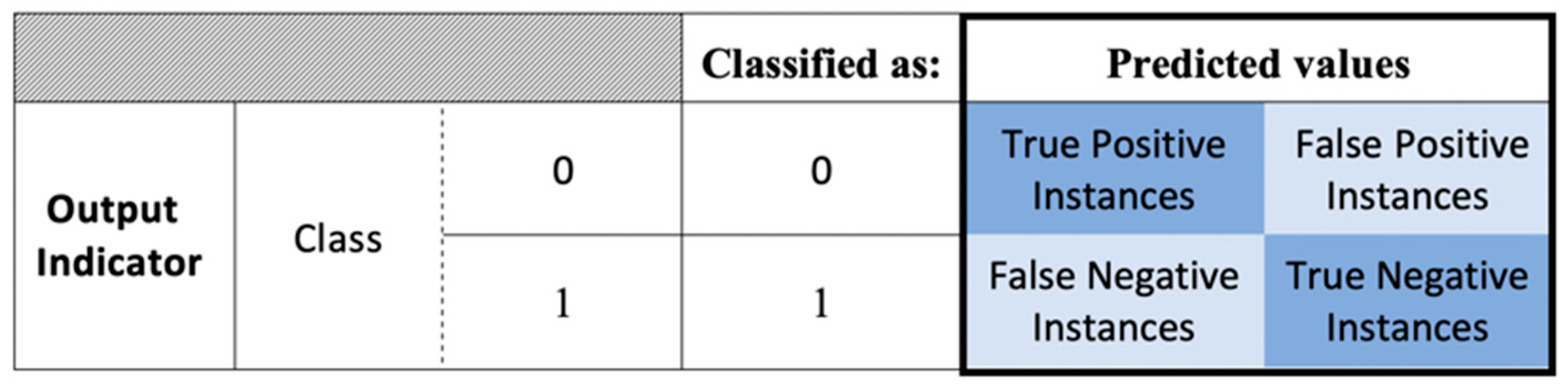
• Confusion matrix: It is a 2 × 2 matrix in which the percentages of true and false instances of each class are presented, with the diagonal elements representing the true instances (true positive and true negative) for each class of the output variable (Figure 1).

Figure 1. The confusion matrix.

Figure 1. The confusion matrix.

A detailed flowchart displaying the entire methodology performed is illustrated in Figure 2.

Figure 2. Flowchart of the methodology performed.

Figure 2. Flowchart of the methodology performed.

3. Results and Discussion

Table 1, Table 2, Table 3, Table 4 and Table 5 present the performance of the machine learning classifiers tested per indicator. Among the hundreds of tests performed aiming at improving performance levels, the best models are the only ones presented, i.e., those with the best performance metrics, along with the highest accuracy scores.

3.1. Prediction of the Indicator “NEPI”

Regarding the prediction of the indicator “NEPI”, almost all classifiers present highly valuable models, with the accuracy score ranging from 87.77% to 94.00% (Table 1). Small differences appear between the models presented, as the performance metrics (precision, recall, F-measure, and ROC area) exceed 0.75 for the weighted average in all models, or even 0.87 if not taking into account the “Lazy IBk” classifier. The correctly predicted instances range between 95% and 97% for the class of the non-energy-poor households and between 57% and 82% for the class of the energy-poor households. Overall, the best performance of the indicator “NEPI” is achieved by the “Random Forest” (94.02%) and the “Multilayer Perceptron” (93.34%) classifiers, with negligible differences between them, followed by “Trees J48” (92.79%), “Rules Decision table” (92.15%), and “Logistic” (91.84%) classifiers (also high predictive models) and, at a longer distance by “Meta AdaBoost M1”, “Naïve Bayes” and “Lazy IBk” classifiers. A graphical interface of classifiers is given indicatively in Figure 3, displaying the ANN (multilayer perceptron) predicting the indicator “NEPI”.

The model resulting from the “Random Forest” classifier presents the best results of the seven classifiers, with an accuracy rate of 94.02%. The performance metrics (precision, recall, F-measure, and ROC area) of this model are remarkably good, exceeding 0.93 for the weighted average. ROC area is equal to 0.97, almost approaching 1.0, implying that the examined model is approaching an ideal model. Similarly, 97% of non-energy-poor households and 81% of energy-poor households are correctly predicted, according to the diagonal elements of the confusion matrix. In the best model, the supervised filter “SMOTE” was used to adapt the relative frequency between majority and minority classes, i.e., increase twofold the instances of the minority class based on the k-nearest neighbor method (10 nearest neighbors selected), and then the unsupervised filter “Randomize” was used in order to shuffle the order of instances.

When removing the variable of “household income” as an input variable, the predictive power of the model with respect to energy-poor households falls drastically. In more detail, in this case, the “Random Forest” classifier manages to correctly predict only 32% of energy-poor households while maintaining significantly high percentages in terms of correctly predicting the class of non-energy-poor households (95%), according to the confusion matrix. This model presents an overall accuracy score of 83.67% and good performance metrics (precision, recall, F-measure, and ROC area), exceeding 0.79 for the weighted average, yet it is regarded as an unreliable model due to the extremely low rates of the second class. The above finding highlights the principal role of income in energy poverty prediction, as without it, the model loses its predictive power of the one class by almost 50 percentage points.

Table 1. Prediction of indicator “NEPI” and confusion matrices (test sets presented).

Prediction of Indicator NEPI–2192 Instances
Classifier	Precision	Recall	F-Measure	ROC Area	Class	Accuracy	Confusion Matrix
Multilayer perceptron	0.959	0.960	0.959	0.973	Non-energy poor	93.34%	96%	4%
	0.820	0.816	0.818	0.973	Energy poor		18%	82%
	0.933	0.933	0.933	0.973	(weighted avg)
Naïve Bayes	0.920	0.937	0.929	0.925	Non-energy poor	88.23%	94%	6%
	0.695	0.639	0.666	0.925	Energy poor		36%	64%
	0.879	0.882	0.880	0.925	(weighted avg)
Rules decision table	0.937	0.969	0.953	0.968	Non-energy poor	92.15%	97%	3%
	0.838	0.709	0.768	0.968	Energy poor		29%	71%
	0.919	0.922	0.919	0.968	(weighted avg)
Meta AdaBoost M1	0.920	0.961	0.940	0.938	Non-energy poor	90.06%	96%	4%
	0.786	0.629	0.699	0.938	Energy poor		37%	63%
	0.896	0.901	0.896	0.938	(weighted avg)
Logistic	0.939	0.963	0.951	0.968	Non-energy poor	91.84%	96%	4%
	0.812	0.721	0.764	0.968	Energy poor		28%	72%
	0.916	0.918	0.916	0.968	(weighted avg)
Trees J48	0.947	0.965	0.956	0.923	Non-energy poor	92.79%	97%	3%
	0.832	0.761	0.795	0.923	Energy poor		24%	76%
	0.926	0.928	0.927	0.923	(weighted avg)
Lazy IBk	0.907	0.947	0.927	0.758	Non-energy poor	87.77%	95%	5%
	0.707	0.570	0.631	0.758	Energy poor		43%	57%
	0.871	0.878	0.872	0.758	(weighted avg)
Random forest	0.958	0.969	0.964	0.971	Non-energy poor	94.02%	97%	3%
	0.856	0.811	0.833	0.971	Energy poor		19%	81%
	0.939	0.940	0.940	0.971	(weighted avg)

Table 1. Prediction of indicator “NEPI” and confusion matrices (test sets presented).

Prediction of Indicator NEPI–2192 Instances
Classifier	Precision	Recall	F-Measure	ROC Area	Class	Accuracy	Confusion Matrix
Multilayer perceptron	0.959	0.960	0.959	0.973	Non-energy poor	93.34%	96%	4%
	0.820	0.816	0.818	0.973	Energy poor		18%	82%
	0.933	0.933	0.933	0.973	(weighted avg)
Naïve Bayes	0.920	0.937	0.929	0.925	Non-energy poor	88.23%	94%	6%
	0.695	0.639	0.666	0.925	Energy poor		36%	64%
	0.879	0.882	0.880	0.925	(weighted avg)
Rules decision table	0.937	0.969	0.953	0.968	Non-energy poor	92.15%	97%	3%
	0.838	0.709	0.768	0.968	Energy poor		29%	71%
	0.919	0.922	0.919	0.968	(weighted avg)
Meta AdaBoost M1	0.920	0.961	0.940	0.938	Non-energy poor	90.06%	96%	4%
	0.786	0.629	0.699	0.938	Energy poor		37%	63%
	0.896	0.901	0.896	0.938	(weighted avg)
Logistic	0.939	0.963	0.951	0.968	Non-energy poor	91.84%	96%	4%
	0.812	0.721	0.764	0.968	Energy poor		28%	72%
	0.916	0.918	0.916	0.968	(weighted avg)
Trees J48	0.947	0.965	0.956	0.923	Non-energy poor	92.79%	97%	3%
	0.832	0.761	0.795	0.923	Energy poor		24%	76%
	0.926	0.928	0.927	0.923	(weighted avg)
Lazy IBk	0.907	0.947	0.927	0.758	Non-energy poor	87.77%	95%	5%
	0.707	0.570	0.631	0.758	Energy poor		43%	57%
	0.871	0.878	0.872	0.758	(weighted avg)
Random forest	0.958	0.969	0.964	0.971	Non-energy poor	94.02%	97%	3%
	0.856	0.811	0.833	0.971	Energy poor		19%	81%
	0.939	0.940	0.940	0.971	(weighted avg)

In other words, the “Random Forest” classifier, using the eight (8) input socio-economic/technical variables, i.e., household income, household size, house area, heating fuel cost, heating system efficiency, presence of elderly people, presence of unemployed people, and building U-factor, can correctly predict energy poverty, as being defined by the indicator “NEPI”, at a remarkably good level (correct prediction of energy-poor households of 81%), with the overall accuracy rate of the model reaching 93.34%.

Compared with previous relevant research, Papada and Kaliampakos [21] used a neural network (multilayer perceptron classifier) to predict the same output variable (NEPI) in Greece with the same machine learning tool (WEKA), using as independent variables socio-economic/geographical factors, i.e., household size, house area, house age, ownership status, and elevation. The best model of these tests showed an overall accuracy score lower compared to the present outcomes of the “Random Forest” classifier (82.72% vs. 93.34%) and lower performance metrics (over 0.82 vs. over 0.93 of the present model for the weighted average of all metrics). As per the confusion matrix, the best model of [32] showed fewer correct predictions, i.e., 73% vs. 82% for the class of energy-poor households and 88% vs. 96% for the class of non-energy-poor households. The two models are comparable as they use the same methodology for predicting the same indicator but different samples and different input variables. Overall, the performance of the present model is significantly higher, probably because of the use of more (in number) and more detailed input variables.

3.2. Prediction of the Indicator “Modified NEPI”

As regards the prediction of the indicator “modified NEPI”, highly valuable models arise, as also was the case with the “NEPI” indicator. More precisely, all classifiers present high accuracy scores, ranging from 86.62% to 94.45% (Table 2). Small differences appear between most of the models presented, as the performance metrics (precision, recall, F-measure, and ROC area) exceed 0.77 for the weighted average in all models, or even 0.87 if not taking into account the “Lazy IBk” classifier. The correctly predicted instances range between 93% and 97% for the class of non-energy-poor households and between 57% and 83% for the class of energy-poor households. Overall, the best performance of the indicator “modified NEPI” is achieved by the “Random Forest” (94.45%) and “Trees J48” (93.36%) classifiers with negligible differences between them, followed by “Multilayer Perceptron” (92.54%), “Logistic” (92.30%), and “Rules Decision table” (91.53%) classifiers (also high predictive models) and, at a longer distance, by “Meta AdaBoost M1”, “Naïve Bayes”, and “Lazy IBk” classifiers.

The model resulting from the use of the “Random Forest” classifier presents the best results, with an accuracy rate of 94.45%. The performance metrics (precision, recall, F-measure, and ROC area) are remarkably good, exceeding 0.94 for the weighted average. ROC area equals 0.98, almost approaching the ideal unit of 1.0. Similarly, 97% of non-energy-poor households and 83% of energy-poor households are correctly predicted, according to the diagonal elements of the confusion matrix. In the best model, the supervised filter “SMOTE” was used to adapt the relative frequency between majority and minority classes, based on the k-nearest neighbor method (10 nearest neighbors selected), and then the unsupervised filter “Randomize” was used in order to shuffle the order of instances.

If removing the variable of “household income” as an input variable, the predictive power of the model for energy-poor households falls drastically, as also was the case with the “NEPI” indicator. Similarly, in the absence of income, the “Random Forest” classifier manages to correctly predict only 37% of energy-poor households, and, despite its impressive predictive power of non-energy-poor households (97%) with an accuracy rate of 85.75%, the model is regarded as unreliable in total.

In other words, the “Random Forest” classifier, using the eight (8) input socio-economic/technical variables, can correctly predict energy poverty, as being defined by the indicator “modified NEPI”, at a remarkably good level (correct prediction of energy-poor households of 83%), with the overall accuracy rate of the model reaching 94.45%.

Table 2. Prediction of indicator “modified NEPI” and confusion matrices (test sets presented).

Prediction of Indicator Modified NEPI–2197 Instances
Classifier	Precision	Recall	F-Measure	ROC Area	Class	Accuracy	Confusion Matrix
Multilayer perceptron	0.947	0.962	0.954	0.972	Non-energy poor	92.54%	96%	4%
	0.826	0.771	0.798	0.972	Energy poor		23%	77%
	0.924	0.925	0.924	0.972	(weighted avg)
Naïve Bayes	0.905	0.932	0.919	0.914	Non-energy poor	86.62%	93%	7%
	0.670	0.587	0.626	0.914	Energy poor		41%	59%
	0.861	0.866	0.863	0.914	(weighted avg)
Rules decision table	0.931	0.967	0.949	0.952	Non-energy poor	91.53%	97%	3%
	0.832	0.697	0.758	0.952	Energy poor		30%	70%
	0.912	0.915	0.912	0.952	(weighted avg)
Meta AdaBoost M1	0.904	0.959	0.931	0.902	Non-energy poor	88.44%	96%	4%
	0.765	0.568	0.652	0.902	Energy poor		43%	57%
	0.878	0.884	0.878	0.902	(weighted avg)
Logistic	0.940	0.966	0.953	0.970	Non-energy poor	92.30%	97%	3%
	0.838	0.740	0.786	0.970	Energy poor		26%	74%
	0.921	0.923	0.921	0.970	(weighted avg)
Trees J48	0.956	0.962	0.959	0.945	Non-energy poor	93.36%	96%	4%
	0.834	0.814	0.824	0.945	Energy poor		19%	81%
	0.933	0.934	0.933	0.945	(weighted avg)
Lazy IBk	0.909	0.943	0.926	0.774	Non-energy poor	87.80%	94%	6%
	0.714	0.601	0.653	0.774	Energy poor		40%	60%
	0.872	0.878	0.874	0.774	(weighted avg)
Random forest	0.960	0.972	0.966	0.975	Non-energy poor	94.45%	97%	3%
	0.874	0.828	0.850	0.975	Energy poor		17%	83%
	0.944	0.944	0.944	0.975	(weighted avg)

Table 2. Prediction of indicator “modified NEPI” and confusion matrices (test sets presented).

Prediction of Indicator Modified NEPI–2197 Instances
Classifier	Precision	Recall	F-Measure	ROC Area	Class	Accuracy	Confusion Matrix
Multilayer perceptron	0.947	0.962	0.954	0.972	Non-energy poor	92.54%	96%	4%
	0.826	0.771	0.798	0.972	Energy poor		23%	77%
	0.924	0.925	0.924	0.972	(weighted avg)
Naïve Bayes	0.905	0.932	0.919	0.914	Non-energy poor	86.62%	93%	7%
	0.670	0.587	0.626	0.914	Energy poor		41%	59%
	0.861	0.866	0.863	0.914	(weighted avg)
Rules decision table	0.931	0.967	0.949	0.952	Non-energy poor	91.53%	97%	3%
	0.832	0.697	0.758	0.952	Energy poor		30%	70%
	0.912	0.915	0.912	0.952	(weighted avg)
Meta AdaBoost M1	0.904	0.959	0.931	0.902	Non-energy poor	88.44%	96%	4%
	0.765	0.568	0.652	0.902	Energy poor		43%	57%
	0.878	0.884	0.878	0.902	(weighted avg)
Logistic	0.940	0.966	0.953	0.970	Non-energy poor	92.30%	97%	3%
	0.838	0.740	0.786	0.970	Energy poor		26%	74%
	0.921	0.923	0.921	0.970	(weighted avg)
Trees J48	0.956	0.962	0.959	0.945	Non-energy poor	93.36%	96%	4%
	0.834	0.814	0.824	0.945	Energy poor		19%	81%
	0.933	0.934	0.933	0.945	(weighted avg)
Lazy IBk	0.909	0.943	0.926	0.774	Non-energy poor	87.80%	94%	6%
	0.714	0.601	0.653	0.774	Energy poor		40%	60%
	0.872	0.878	0.874	0.774	(weighted avg)
Random forest	0.960	0.972	0.966	0.975	Non-energy poor	94.45%	97%	3%
	0.874	0.828	0.850	0.975	Energy poor		17%	83%
	0.944	0.944	0.944	0.975	(weighted avg)

3.3. Prediction of the Indicator “2M”

Regarding the prediction of the indicator “2M”, classifiers present reasonable models, with high accuracy scores but average correct predictions of the class of energy-poor households. More precisely, the accuracy score ranges from 93.34% to 97.24% (Table 3), while the performance metrics (precision, recall, F-measure, and ROC area) exceed 0.71 for the weighted average in all models, or even 0.86 if not taking into account the “Lazy IBk” classifier. The confusion matrix provides remarkably high values for the class of non-energy-poor households in all models (of the order of 98–100%), but average rates for the class of energy-poor households (43% to 65%). As a result, the models derived from “Naïve Bayes”, “Lazy IBk”, and “Logistic” classifiers are considered non-meaningful at all, due to the low rates (below and around 50%) of the confusion matrix of the second class.

Overall, the best performance of the indicator “2M” is achieved by the “Rules Decision table” (97.24%) and the “Random Forest” (96.70%) classifiers with minor differences between them, followed by “Trees J48” (96.00%), “Meta AdaBoost M1” (95.34%), and “Multilayer Perceptron” (93.34%) classifiers.

Table 3. Prediction of indicator “2M” and confusion matrices (test sets presented).

Prediction of Indicator 2M–2062 Instances
Classifier	Precision	Recall	F-Measure	ROC Area	Class	Accuracy	Confusion Matrix
Multilayer perceptron	0.968	0.986	0.977	0.934	Non-energy poor	93.34%	99%	1%
	0.772	0.587	0.667	0.934	Energy poor		41%	59%
	0.954	0.957	0.955	0.934	(weighted avg)
Naïve Bayes	0.957	0.983	0.970	0.914	Non-energy poor	94.33%	98%	2%
	0.670	0.433	0.526	0.914	Energy poor		57%	43%
	0.936	0.943	0.938	0.914	(weighted avg)
Rules decision table	0.973	0.997	0.985	0.965	Non-energy poor	97.24%	100%	0%
	0.951	0.653	0.775	0.965	Energy poor		35%	65%
	0.972	0.972	0.970	0.965	(weighted avg)
Meta AdaBoost M1	0.968	0.983	0.975	0.928	Non-energy poor	95.34%	98%	2%
	0.725	0.580	0.644	0.928	Energy poor		42%	58%
	0.950	0.953	0.951	0.928	(weighted avg)
Logistic	0.963	0.989	0.976	0.944	Non-energy poor	95.49%	99%	1%
	0.788	0.520	0.627	0.944	Energy poor		48%	52%
	0.951	0.955	0.951	0.944	(weighted avg)
Trees J48	0.967	0.985	0.976	0.865	Non-energy poor	95.54%	99%	1%
	0.754	0.573	0.652	0.865	Energy poor		43%	57%
	0.952	0.955	0.953	0.865	(weighted avg)
Lazy IBk	0.960	0.979	0.969	0.716	Non-energy poor	94.23%	98%	2%
	0.640	0.473	0.544	0.716	Energy poor		53%	47%
	0.936	0.942	0.938	0.716	(weighted avg)
Random forest	0.971	0.994	0.982	0.942	Non-energy poor	96.70%	99%	1%
	0.894	0.620	0.732	0.942	Energy poor		38%	62%
	0.965	0.967	0.964	0.942	(weighted avg)

Table 3. Prediction of indicator “2M” and confusion matrices (test sets presented).

Prediction of Indicator 2M–2062 Instances
Classifier	Precision	Recall	F-Measure	ROC Area	Class	Accuracy	Confusion Matrix
Multilayer perceptron	0.968	0.986	0.977	0.934	Non-energy poor	93.34%	99%	1%
	0.772	0.587	0.667	0.934	Energy poor		41%	59%
	0.954	0.957	0.955	0.934	(weighted avg)
Naïve Bayes	0.957	0.983	0.970	0.914	Non-energy poor	94.33%	98%	2%
	0.670	0.433	0.526	0.914	Energy poor		57%	43%
	0.936	0.943	0.938	0.914	(weighted avg)
Rules decision table	0.973	0.997	0.985	0.965	Non-energy poor	97.24%	100%	0%
	0.951	0.653	0.775	0.965	Energy poor		35%	65%
	0.972	0.972	0.970	0.965	(weighted avg)
Meta AdaBoost M1	0.968	0.983	0.975	0.928	Non-energy poor	95.34%	98%	2%
	0.725	0.580	0.644	0.928	Energy poor		42%	58%
	0.950	0.953	0.951	0.928	(weighted avg)
Logistic	0.963	0.989	0.976	0.944	Non-energy poor	95.49%	99%	1%
	0.788	0.520	0.627	0.944	Energy poor		48%	52%
	0.951	0.955	0.951	0.944	(weighted avg)
Trees J48	0.967	0.985	0.976	0.865	Non-energy poor	95.54%	99%	1%
	0.754	0.573	0.652	0.865	Energy poor		43%	57%
	0.952	0.955	0.953	0.865	(weighted avg)
Lazy IBk	0.960	0.979	0.969	0.716	Non-energy poor	94.23%	98%	2%
	0.640	0.473	0.544	0.716	Energy poor		53%	47%
	0.936	0.942	0.938	0.716	(weighted avg)
Random forest	0.971	0.994	0.982	0.942	Non-energy poor	96.70%	99%	1%
	0.894	0.620	0.732	0.942	Energy poor		38%	62%
	0.965	0.967	0.964	0.942	(weighted avg)

The model resulting from the use of the “Rules Decision table” classifier displays the best results, with an accuracy rate of 97.24%. The performance metrics (precision, recall, F-measure, and ROC area) are remarkably good, exceeding 0.96 for the weighted average. ROC area is equal to 0.97, implying that the examined model is almost an ideal model. Similarly, as per the diagonal parts of the confusion matrix, 100% of non-energy-poor households and 65% of energy-poor households are correctly predicted. In the best model, the supervised filter “SMOTE” was used to adapt the relative frequency between majority and minority classes, based on the k-nearest neighbor method (10 nearest neighbors selected), and then the unsupervised filter “Randomize” was used in order to shuffle the order of instances.

The best model was also tested for the case of removing the variable of “household income” as an input variable. The findings of the previous indicators—in terms of the crucial role of income in energy poverty prediction—were once again validated, as the new model without income manages to correctly predict only 31% of energy-poor households; hence, it is regarded as unreliable in total.

In other words, the “Rules Decision table” classifier, using the eight (8) input socio-economic/technical variables selected, can correctly predict energy poverty, as being defined by the indicator “2M”, at a moderately satisfactory level (correct prediction of energy-poor households of 65%), with the overall accuracy rate of the model reaching 97.24%.

3.4. Prediction of the Indicator “M/2”

As regards the prediction of the indicator “M/2”, almost all classifiers present unreasonable models, with satisfactory and high accuracy scores but particularly low correct predictions of the second class (energy-poor households). More precisely, the accuracy score ranges from 75.46% to 86.81% (Table 4), and the performance metrics (precision, recall, F-measure, and ROC area) exceed 0.69 for the weighted average in all models.

Table 4. Prediction of indicator “M/2” and confusion matrices (test sets presented).

Prediction of Indicator M/2–2274 Instances
Classifier	Precision	Recall	F-Measure	ROC Area	Class	Accuracy	Confusion Matrix
Multilayer perceptron	0.831	0.982	0.900	0.809	Non-energy poor	83.47%	98%	2%
	0.869	0.373	0.522	0.809	Energy poor		63%	37%
	0.840	0.835	0.809	0.809	(weighted avg)
Naïve Bayes	0.819	0.869	0.843	0.709	Non-energy poor	75.46%	87%	13%
	0.491	0.396	0.439	0.709	Energy poor		60%	40%
	0.739	0.755	0.745	0.709	(weighted avg)
Rules decision table	0.857	0.983	0.916	0.846	Non-energy poor	86.28%	98%	2%
	0.902	0.485	0.631	0.846	Energy poor		51%	49%
	0.868	0.863	0.847	0.846	(weighted avg)
Meta AdaBoost M1	0.814	0.966	0.884	0.818	Non-energy poor	80.74%	97%	3%
	0.746	0.309	0.437	0.818	Energy poor		69%	31%
	0.798	0.807	0.776	0.818	(weighted avg)
Logistic	0.790	0.950	0.862	0.725	Non-energy poor	77.00%	95%	5%
	0.567	0.207	0.304	0.725	Energy poor		79%	21%
	0.736	0.770	0.727	0.725	(weighted avg)
Trees J48	0.865	0.934	0.898	0.818	Non-energy poor	83.95%	93%	7%
	0.724	0.544	0.621	0.818	Energy poor		46%	54%
	0.831	0.839	0.831	0.818	(weighted avg)
Lazy IBk	0.852	0.861	0.857	0.697	Non-energy poor	78.14%	86%	14%
	0.550	0.533	0.541	0.697	Energy poor		47%	53%
	0.779	0.781	0.780	0.697	(weighted avg)
Random forest	0.876	0.963	0.917	0.875	Non-energy poor	86.81%	96%	4%
	0.831	0.571	0.677	0.875	Energy poor		43%	57%
	0.865	0.868	0.859	0.875	(weighted avg)

Table 4. Prediction of indicator “M/2” and confusion matrices (test sets presented).

Prediction of Indicator M/2–2274 Instances
Classifier	Precision	Recall	F-Measure	ROC Area	Class	Accuracy	Confusion Matrix
Multilayer perceptron	0.831	0.982	0.900	0.809	Non-energy poor	83.47%	98%	2%
	0.869	0.373	0.522	0.809	Energy poor		63%	37%
	0.840	0.835	0.809	0.809	(weighted avg)
Naïve Bayes	0.819	0.869	0.843	0.709	Non-energy poor	75.46%	87%	13%
	0.491	0.396	0.439	0.709	Energy poor		60%	40%
	0.739	0.755	0.745	0.709	(weighted avg)
Rules decision table	0.857	0.983	0.916	0.846	Non-energy poor	86.28%	98%	2%
	0.902	0.485	0.631	0.846	Energy poor		51%	49%
	0.868	0.863	0.847	0.846	(weighted avg)
Meta AdaBoost M1	0.814	0.966	0.884	0.818	Non-energy poor	80.74%	97%	3%
	0.746	0.309	0.437	0.818	Energy poor		69%	31%
	0.798	0.807	0.776	0.818	(weighted avg)
Logistic	0.790	0.950	0.862	0.725	Non-energy poor	77.00%	95%	5%
	0.567	0.207	0.304	0.725	Energy poor		79%	21%
	0.736	0.770	0.727	0.725	(weighted avg)
Trees J48	0.865	0.934	0.898	0.818	Non-energy poor	83.95%	93%	7%
	0.724	0.544	0.621	0.818	Energy poor		46%	54%
	0.831	0.839	0.831	0.818	(weighted avg)
Lazy IBk	0.852	0.861	0.857	0.697	Non-energy poor	78.14%	86%	14%
	0.550	0.533	0.541	0.697	Energy poor		47%	53%
	0.779	0.781	0.780	0.697	(weighted avg)
Random forest	0.876	0.963	0.917	0.875	Non-energy poor	86.81%	96%	4%
	0.831	0.571	0.677	0.875	Energy poor		43%	57%
	0.865	0.868	0.859	0.875	(weighted avg)

The confusion matrix provides high rates for the class of non-energy-poor households in all models (86% to 98%), but considerably low rates for the class of energy-poor households (21% to 57%). As a result, the models derived from almost all classifiers, i.e., “Logistic”, “Meta AdaBoost M1”, “Multilayer Perceptron”, “Naïve Bayes”, “Rules Decision table”, and “Lazy IBk” classifiers, are considered non-meaningful at all, due to the low rates (below and around 50%) of the confusion matrix of the second class.

The models resulting from the “Random Forest” and “Trees J48” classifiers are the only ones acceptable, both presenting high accuracy scores (86.81% and 83.95%, respectively) but low correct predictions of the second class (57% and 54%, respectively). Especially the “Random Forest” classifier displays the best results between the two, with an accuracy rate of 86.81% and good performance metrics (precision, recall, F-measure, and ROC area), exceeding 0.85 for the weighted average. In this model, 96% of non-energy-poor households and 57% of energy-poor households are correctly predicted, according to the diagonal parts of the confusion matrix. In this model, the supervised filter “SMOTE” was used to adapt the relative frequency between majority and minority classes, i.e., increase twofold the instances of the minority class based on the k-nearest neighbor method (10 nearest neighbors selected), and then the unsupervised filter “Randomize” was used to shuffle the order of instances. When removing the input variable of “household income”, the new model—without income—manages to correctly predict even fewer energy-poor households (49%), which is not meaningful at all.

In other words, the “Random Forest” classifier, using the eight (8) input socio-economic/technical variables selected, can correctly predict energy poverty, as being defined by the indicator “M/2”, at a marginally accepted level (correct prediction of energy-poor households of 57%), with the overall accuracy rate of the model reaching 86.81%. Practically, this model fails to successfully predict energy poverty as being defined by the indicator “M/2”.

3.5. Prediction of the Indicator “Modified LIHC”

Regarding the prediction of the indicator “modified LIHC”, all classifiers present highly valuable models, with the accuracy score ranging from 84.84% to 96.37% (Table 5). Small differences appear between the models presented, as the performance metrics (precision, recall, F-measure, and ROC area) are considerably good, exceeding 0.84 for the weighted average in all models. The correctly predicted instances range between 86% and 97% for the class of non-energy-poor households and between 80% and 97% for the class of energy-poor households. Although differences are slight, overall, the best performance of the indicator “modified LIHC” is achieved by the “Random Forest” classifier (96.37%), followed by “Trees J48” (95.47%), “Multilayer Perceptron” (94.69%), and “Logistic” (94.69%) classifiers and subsequently by “Rules Decision table” (93.33%), Meta AdaBoost M1” (89.45%), “Lazy IBk” (89.37%), and “Naïve Bayes” classifiers (84.84%).

The model resulting from the “Random Forest” classifier presents the best results of the seven classifiers, with an accuracy rate of 96.37%. The performance metrics (precision, recall, F-measure, and ROC area) are remarkably good, exceeding 0.96 for the weighted average. ROC area is equal to 0.99, i.e., an ideal model in terms of random classification. Similarly, 97% of non-energy-poor households and 94% of energy-poor households are correctly predicted, according to the diagonal elements of the confusion matrix. The supervised filter “SMOTE” was used to adapt the relative frequency between majority and minority classes based on the k-nearest neighbor method (10 nearest neighbors selected), and then the unsupervised filter “Randomize” was used to shuffle the order of instances.

When removing the input variable of “household income”, the predictive power of the model with respect to energy-poor households falls considerably, as happened with all previous indicators. Hence, in the absence of income, the model manages to correctly predict 64% of energy-poor households and 87% of non-energy-poor households, with an accuracy rate of 78.90%, which is accepted as a model according to metrics, but it is far less valuable compared to the case of incorporating “household income” as an input variable.

In other words, the “Random Forest” classifier, using the eight (8) input socio-economic/technical variables selected, can correctly predict energy poverty, as being defined by the indicator “modified LIHC” at a remarkably good level (correct prediction of energy-poor households of 94%), with the overall accuracy rate of the model reaching 96.37%.

Comparing with previous relevant research, a similar decision tree classifier (Random Forest) was employed by Al Kez et al. [26] in order to predict—not the same but—a similar energy poverty indicator in the UK (the “LILEE indicator”, or low income low energy efficiency). This model, which used as input variables income, efficiency, and eight (8) additional variables, presented an impressive accuracy score close to 100%, but when income and efficiency were excluded from the model, the accuracy score decreased to 67%. The rates are very close to those of the present paper, confirming the great performance of a decision tree (especially of “Random Forest”) classifier in energy poverty prediction, as well as the decisive role of income in energy poverty prediction via machine learning.

Table 5. Prediction of indicator “modified LIHC” and confusion matrices (test sets presented).

Prediction of Indicator Modified LIHC–2427 Instances
Classifier	Precision	Recall	F-Measure	ROC Area	Class	Accuracy	Confusion Matrix
Multilayer perceptron	0.983	0.936	0.959	0.991	Non-energy poor	94.69%	94%	6%
	0.885	0.968	0.924	0.991	Energy poor		3%	97%
	0.950	0.947	0.947	0.991	(weighted avg)
Naïve Bayes	0.903	0.864	0.883	0.913	Non-energy poor	84.84%	86%	14%
	0.753	0.817	0.784	0.913	Energy poor		18%	82%
	0.853	0.848	0.850	0.913	(weighted avg)
Rules decision table	0.940	0.960	0.950	0.982	Non-energy poor	93.33%	96%	4%
	0.918	0.880	0.898	0.982	Energy poor		12%	88%
	0.933	0.933	0.933	0.982	(weighted avg)
Meta AdaBoost M1	0.962	0.876	0.917	0.973	Non-energy poor	89.45%	88%	12%
	0.791	0.931	0.856	0.973	Energy poor		7%	93%
	0.905	0.895	0.896	0.973	(weighted avg)
Logistic	0.959	0.961	0.960	0.987	Non-energy poor	94.69%	96%	4%
	0.922	0.919	0.921	0.987	Energy poor		8%	92%
	0.947	0.947	0.947	0.987	(weighted avg)
Trees J48	0.969	0.962	0.966	0.968	Non-energy poor	95.47%	96%	4%
	0.926	0.940	0.933	0.968	Energy poor		6%	94%
	0.955	0.955	0.955	0.968	(weighted avg)
Lazy IBk	0.904	0.939	0.921	0.871	Non-energy poor	89.37%	94%	6%
	0.870	0.804	0.835	0.871	Energy poor		20%	80%
	0.893	0.894	0.893	0.871	(weighted avg)
Random forest	0.972	0.974	0.973	0.994	Non-energy poor	96.37%	97%	3%
	0.948	0.944	0.946	0.994	Energy poor		6%	94%
	0.964	0.964	0.964	0.994	(weighted avg)

Table 5. Prediction of indicator “modified LIHC” and confusion matrices (test sets presented).

Prediction of Indicator Modified LIHC–2427 Instances
Classifier	Precision	Recall	F-Measure	ROC Area	Class	Accuracy	Confusion Matrix
Multilayer perceptron	0.983	0.936	0.959	0.991	Non-energy poor	94.69%	94%	6%
	0.885	0.968	0.924	0.991	Energy poor		3%	97%
	0.950	0.947	0.947	0.991	(weighted avg)
Naïve Bayes	0.903	0.864	0.883	0.913	Non-energy poor	84.84%	86%	14%
	0.753	0.817	0.784	0.913	Energy poor		18%	82%
	0.853	0.848	0.850	0.913	(weighted avg)
Rules decision table	0.940	0.960	0.950	0.982	Non-energy poor	93.33%	96%	4%
	0.918	0.880	0.898	0.982	Energy poor		12%	88%
	0.933	0.933	0.933	0.982	(weighted avg)
Meta AdaBoost M1	0.962	0.876	0.917	0.973	Non-energy poor	89.45%	88%	12%
	0.791	0.931	0.856	0.973	Energy poor		7%	93%
	0.905	0.895	0.896	0.973	(weighted avg)
Logistic	0.959	0.961	0.960	0.987	Non-energy poor	94.69%	96%	4%
	0.922	0.919	0.921	0.987	Energy poor		8%	92%
	0.947	0.947	0.947	0.987	(weighted avg)
Trees J48	0.969	0.962	0.966	0.968	Non-energy poor	95.47%	96%	4%
	0.926	0.940	0.933	0.968	Energy poor		6%	94%
	0.955	0.955	0.955	0.968	(weighted avg)
Lazy IBk	0.904	0.939	0.921	0.871	Non-energy poor	89.37%	94%	6%
	0.870	0.804	0.835	0.871	Energy poor		20%	80%
	0.893	0.894	0.893	0.871	(weighted avg)
Random forest	0.972	0.974	0.973	0.994	Non-energy poor	96.37%	97%	3%
	0.948	0.944	0.946	0.994	Energy poor		6%	94%
	0.964	0.964	0.964	0.994	(weighted avg)

4. Conclusions

The present research enlightens an innovative practice of analyzing energy poverty, i.e., machine learning. A distinctive aspect of the research is that a model is authorized to learn from real data on how to weight the selected drivers/variables and determine their interrelationships, contrary to traditional statistical techniques in which the weighting of variables is a prerequisite for running a model. Hence, the present work addresses a gap in the literature regarding the absence of an “established protocol” for weighting drivers of energy poverty, as highlighted by Walker et al. [49] and Longa et al. [25].

The analysis showed that almost all classifiers managed to successfully predict three (3) out of five (5) energy poverty indicators with a high level of accuracy, namely, “NEPI”, “modified NEPI”, and “modified LIHC” (81%, 83%, and 94% correct predictions of energy-poor households of the best models, respectively, with an overall accuracy rate of the models over 94% in all cases). However, considerably lower rates were achieved in the case of “2M” and “M/2” indicators, i.e., 65% and 57% correct predictions of energy-poor households, with 97% and 86% total accuracy scores of the models, respectively. Overall, the most successful classifier in terms of energy poverty prediction proved to be the “Random Forest” classifier (decision tree approach), closely followed by “Trees J48” and “Multilayer Perceptron” classifiers (decision tree and neural network approach, respectively) and, at a longer distance, by “Logistic”, “Rules Decision table”, and “Meta AdaBoost M1” classifiers. The weakest classifiers, or else, classifiers with the lowest performance, proved to be “Lazy IBk” and “Naïve Bayes” classifiers.

Another interesting finding is the validation of the principal role of income in energy poverty prediction when applying machine learning techniques. More specifically, when removing the variable of “household income” from the input variables, the predictive power of the best models concerning energy-poor households drops drastically in almost all cases (by 30–50 percentage points, accompanied also by a total lower accuracy score of the models). With the inclusion of income, though, “Random Forest”, “Trees J48”, and “Multilayer Perceptron” classifiers presented an impressive performance, achieving particularly high success rates.

Moreover, it is noteworthy that, although numerous different types of classifiers were tested in terms of their characteristics, the best results were reached by their simplest types, e.g., by selecting one (1) instead of two (2) or more hidden layers in the “Multilayer Perceptron” classifier, etc. Furthermore, the filter “SMOTE” was applied to all cases, again through numerous tests of the filter’s characteristics, in order to adapt the relative frequency between majority and minority classes and thus minimize bias in the results.

The particularly high prediction rates and accuracy scores that came up in the study area confirmed that ML algorithms could be a useful tool in terms of detecting energy poverty roots, without knowing their exact relationships with the problem. This information can in turn benefit decision-making. Practically, the present research showed that eight (8) specific socio-economic/technical variables, i.e., household income, household size, house area, heating fuel cost, heating system efficiency, presence of elderly people, presence of unemployed people, and building U-factor, are of particular importance when combined all together, as they can accurately predict energy poverty by over 80%. By this means, machine learning can serve as a valuable policy tool for decision-makers, in order to spot vulnerable households and, hence, take more focused policy measures, e.g., lower energy prices, tax reliefs, allowances, motives towards upgrading the building’s energy performance, etc.

As regards future research, one possible direction would include the exploration of whether the high rates of the predictive models or the predictors themselves would significantly change depending on the sample, i.e., by testing different study areas/countries with various geographical characteristics that could affect energy poverty in different ways, such as mountainous areas, lowlands, island areas, etc. In any case, due to the exact complex nature of energy poverty, machine learning seems to be a promising tool towards experimenting quickly with large amounts of data (variables/characteristics/causes of the problem) and shaping appropriate energy policies.

References

- IEA. SDG7: Data and Projections. 2023. Available online: https://www.iea.org/reports/sdg7-data-and-projections (accessed on 19 December 2024).
- Samarakoon, S. A justice and wellbeing centered framework for analysing energy poverty in the Global South. Ecol. Econ. 2019, 165, 106385. [Google Scholar] [CrossRef]
- Hesselman, M.; Varo, A.; Guyet, R.; Thomson, H. Energy poverty in the COVID-19 era: Mapping global responses in light of momentum for the right to energy. Energy Res. Soc. Sci. 2021, 81, 102246. [Google Scholar] [CrossRef] [PubMed]
- Carfora, A.; Scandurra, G.; Thomas, A. Forecasting the COVID-19 effects on energy poverty across EU member states. Energy Policy 2022, 161, 112597. [Google Scholar] [CrossRef] [PubMed]
- Baker, S.H.; Carley, S.; Konisky, D.M. Energy insecurity and the urgent need for utility disconnection protections. Energy Policy 2021, 159, 112663. [Google Scholar] [CrossRef]
- Clark, I.; Chun, S.; O’Sullivan, K.; Pierse, N. Energy Poverty among Tertiary Students in Aotearoa New Zealand. Energies 2021, 15, 76. [Google Scholar] [CrossRef]
- Papada, L.; Kaliampakos, D. A Stochastic Model for energy poverty analysis. Energy Policy 2018, 116, 153–164. [Google Scholar] [CrossRef]
- Eurostat. People at Risk of Poverty or Social Exclusion. 2023. Available online: https://ec.europa.eu/eurostat/databrowser/view/sdg_01_10/default/table?lang=en (accessed on 19 December 2024).
- Atsalis, A.; Mirasgedis, S.; Tourkolias, C.; Diakoulaki, D. Fuel poverty in Greece: Quantitative analysis and implications for policy. Energy Build. 2016, 131, 87–98. [Google Scholar] [CrossRef]
- Papada, L.; Kaliampakos, D. Measuring energy poverty in Greece. Energy Policy 2016, 94, 157–165. [Google Scholar] [CrossRef]
- Papada, L.; Kaliampakos, D. Energy poverty in Greek mountainous areas: A comparative study. J. Mt. Sci. 2017, 14, 1229–1240. [Google Scholar] [CrossRef]
- Spiliotis, E.; Arsenopoulos, A.; Kanellou, E.; Psarras, J.; Kontogiorgos, P. A multi-sourced data based framework for assisting utilities identify energy poor households: A case-study in Greece. Energy Sources Part B Econ. Plan. Policy 2020, 15, 49–71. [Google Scholar] [CrossRef]
- Kalfountzou, E.; Tourkolias, C.; Mirasgedis, S.; Damigos, D. Identifying Energy-Poor Households with Publicly Available Information: Promising Practices and Lessons Learned from the Athens Urban Area, Greece. Energies 2024, 17, 919. [Google Scholar] [CrossRef]
- Ntaintasis, E.; Mirasgedis, S.; Tourkolias, C. Comparing different methodological approaches for measuring energy poverty: Evidence from a survey in the region of Attika, Greece. Energy Policy 2019, 125, 160–169. [Google Scholar] [CrossRef]
- Boemi, S.-N.; Avdimiotis, S.; Papadopoulos, A.M. Domestic energy deprivation in Greece: A field study. Energy Build. 2017, 144, 167–174. [Google Scholar] [CrossRef]
- Palmos Analysis. Thessaloniki: 190,000 Households Vulnerable or in a State of Energy Poverty. Available online: https://parallaximag.gr/life/energiaki-ftochia-stopoleodomiko-sigkrotima-thessalonikis (accessed on 20 December 2024).
- Papada, L.; Kaliampakos, D. Being forced to skimp on energy needs: A new look at energy poverty in Greece. Energy Res. Soc. Sci. 2020, 64, 101450. [Google Scholar] [CrossRef]
- Lyra, K.; Mirasgedis, S.; Tourkolias, C. From measuring fuel poverty to identification of fuel poor households: A case study in Greece. Energy Effic. 2022, 15, 6. [Google Scholar] [CrossRef]
- Kalfountzou, E.; Papada, L.; Damigos, D.; Degiannakis, S. Predicting energy poverty in Greece through statistical data analysis. Int. J. Sustain. Energy 2022, 41, 1605–1622. [Google Scholar] [CrossRef]
- Halkos, G.; Kostakis, I. Exploring the persistence and transience of energy poverty: Evidence from a Greek household survey. Energy Effic. 2023, 16, 50. [Google Scholar] [CrossRef]
- Papada, L.; Kaliampakos, D. Artificial Neural Networks as a Tool to Understand Complex Energy Poverty Relationships: The Case of Greece. Energies 2024, 17, 3163. [Google Scholar] [CrossRef]
- Hong, Z.; Park, I.K. Comparative Analysis of Energy Poverty Prediction Models Using Machine Learning Algorithms. J. Korea Plan. Assoc. 2021, 56, 239–255. [Google Scholar] [CrossRef]
- Hassani, H.; Yeganegi, M.R.; Beneki, C.; Unger, S.; Moradghaffari, M. Big Data and Energy Poverty Alleviation. Big Data Cognit. Comput. 2019, 3, 50. [Google Scholar] [CrossRef]
- López-Vargas, A.; Ledezma-Espino, A.; Sanchis-de-Miguel, A. Methods, data sources and applications of the Artificial Intelligence in the Energy Poverty context: A review. Energy Build. 2022, 268, 112233. [Google Scholar] [CrossRef]
- Dalla Longa, F.; Sweerts, B.; Van Der Zwaan, B. Exploring the complex origins of energy poverty in The Netherlands with machine learning. Energy Policy 2021, 156, 112373. [Google Scholar] [CrossRef]
- Al Kez, D.; Foley, A.; Abdul, Z.K.; Del Rio, D.F. Energy poverty prediction in the United Kingdom: A machine learning approach. Energy Policy 2024, 184, 113909. [Google Scholar] [CrossRef]
- Spandagos, C.; Tovar Reaños, M.A.; Lynch, M.Á. Energy poverty prediction and effective targeting for just transitions with machine learning. Energy Econ. 2023, 128, 107131. [Google Scholar] [CrossRef]
- Van Hove, W.; Dalla Longa, F.; Van Der Zwaan, B. Identifying predictors for energy poverty in Europe using machine learning. Energy Build. 2022, 264, 112064. [Google Scholar] [CrossRef]
- Mukelabai, M.D.; Wijayantha, K.G.U.; Blanchard, R.E. Using machine learning to expound energy poverty in the global south: Understanding and predicting access to cooking with clean energy. Energy AI 2023, 14, 100290. [Google Scholar] [CrossRef]
- Pino-Mejías, R.; Pérez-Fargallo, A.; Rubio-Bellido, C.; Pulido-Arcas, J.A. Artificial neural networks and linear regression prediction models for social housing allocation: Fuel Poverty Potential Risk Index. Energy 2018, 164, 627–641. [Google Scholar] [CrossRef]
- Bienvenido-Huertas, D.; Pérez-Fargallo, A.; Alvarado-Amador, R.; Rubio-Bellido, C. Influence of climate on the creation of multilayer perceptrons to analyse the risk of fuel poverty. Energy Build. 2019, 198, 38–60. [Google Scholar] [CrossRef]
- Papada, L.; Kaliampakos, D. Exploring Energy Poverty Indicators Through Artificial Neural Networks. In Artificial Intelligence and Sustainable Computing; Pandit, M., Gaur, M.K., Rana, P.S., Tiwari, A., Eds.; Algorithms for Intelligent Systems; Springer Nature: Singapore, 2022; pp. 231–242. [Google Scholar] [CrossRef]
- Abbas, K.; Butt, K.M.; Xu, D.; Ali, M.; Baz, K.; Kharl, S.H.; Ahmed, M. Measurements and determinants of extreme multidimensional energy poverty using machine learning. Energy 2022, 251, 123977. [Google Scholar] [CrossRef]
- Gawusu, S.; Jamatutu, S.A.; Ahmed, A. Predictive Modeling of Energy Poverty with Machine Learning Ensembles: Strategic Insights from Socioeconomic Determinants for Effective Policy Implementation. Int. J. Energy Res. 2024, 2024, 9411326. [Google Scholar] [CrossRef]
- Balkissoon, S.; Fox, N.; Lupo, A.; Haupt, S.E.; Penny, S.G.; Miller, S.J.; Beetstra, M.; Sykuta, M.; Ohler, A. Forecasting energy poverty using different machine learning techniques for Missouri. Energy 2024, 313, 133904. [Google Scholar] [CrossRef]
- Grzybowska, U.; Wojewódzka-Wiewiórska, A.; Vaznonienė, G.; Dudek, H. Households Vulnerable to Energy Poverty in the Visegrad Group Countries: An Analysis of Socio-Economic Factors Using a Machine Learning Approach. Energies 2024, 17, 6310. [Google Scholar] [CrossRef]
- Ministry of Development. Liquid Fuel Prices Observatory. Available online: http://www.fuelprices.gr/ (accessed on 7 January 2025). (In Greek).
- General Secretariat of Commerce & Consumer Protection. Refinery Prices. Available online: http://oil.gge.gov.gr/ (accessed on 20 December 2024). (In Greek)
- Ministry of the Environment and Energy. Greek Regulation of Energy Efficiency in Buildings-Τ.Ο.Τ.Ε.Ε. KENAK 20701-1/2017’. 2017. Available online: https://www.kenak.gr/files/TOTEE_20701-1_2017.pdf (accessed on 10 January 2025). (In Greek).
- Frank, E.; Hall, M.A.; Witten, I.H. The WEKA Workbench. Practical Machine Learning Tools and Techniques. In Data Mining, 4th ed.; Morgan Kaufmann: Waikato, New Zealand, 2016. [Google Scholar]
- Kumar, Y. Analysis of Bayes, Neural Network and Tree Classifier of Classification Technique in Data Mining using WEKA. In Proceedings of the Computer Science & Information Technology (CS & IT); Academy & Industry Research Collaboration Center (AIRCC): Chennai, India, 2012; pp. 359–369. [Google Scholar] [CrossRef]
- Hangloo, S.; Kour, S.; Kumar, S. A Survey on Machine Learning: Concept, Algorithms, and Applications. Int. J. Sci. Res. Comput. Sci. Eng. Inf. Technol. (IJSRCSEIT) 2017, 2, 293–301. [Google Scholar]
- Kaur, G.; Chhabra, A. Improved J48 Classification Algorithm for the Prediction of Diabetes. IJCA 2014, 98, 13–17. [Google Scholar] [CrossRef]
- Breiman, L. Random Forests. Mach. Learn. 2001, 45, 5–32. [Google Scholar] [CrossRef]
- Cerquides, J.; de M’antaras, R.L. Maximum a Posteriori Tree Augmented Naive Bayes Classifiers. October 2003. Available online: https://www.iiia.csic.es/~mantaras/ReportIIIA-TR-2003-10.pdf (accessed on 8 January 2025).
- Kalmegh, S.R. Comparative Analysis of the WEKA Classifiers Rules Conjunctiverule & Decisiontable on Indian News Dataset by Using Different Test Mode. Int. J. Eng. Sci. Invent. 2018, 7, 01–09. [Google Scholar]
- Devi, T.; Sundaram, K.M. A comparative analysis of meta and tree classification algorithms using weka. Comput. Sci. 2016, 3, 77–83. [Google Scholar]
- Vijayarani, S.; Muthulakshmi, M. Comparative Analysis of Bayes and Lazy Classification Algorithms. Int. J. Adv. Res. Comput. Commun. Eng. 2013, 2, 3118–3124. [Google Scholar]
- Walker, R.; McKenzie, P.; Liddell, C.; Morris, C. Area-based targeting of fuel poverty in Northern Ireland: An evidenced-based approach. Appl. Geogr. 2012, 34, 639–649. [Google Scholar] [CrossRef]
Disclaimer/Publisher’s Note: The statements, opinions and data contained in all publications are solely those of the individual author(s) and contributor(s) and not of MDPI and/or the editor(s). MDPI and/or the editor(s) disclaim responsibility for any injury to people or property resulting from any ideas, methods, instructions or products referred to in the content. |
© 2025 by the authors. Licensee MDPI, Basel, Switzerland. This article is an open access article distributed under the terms and conditions of the Creative Commons Attribution (CC BY) license (https://creativecommons.org/licenses/by/4.0/).
Share and Cite
Kalfountzou, E.; Papada, L.; Tourkolias, C.; Mirasgedis, S.; Kaliampakos, D.; Damigos, D. A Comparative Analysis of Machine Learning Algorithms in Energy Poverty Prediction. Energies 2025, 18, 1133. https://doi.org/10.3390/en18051133
Kalfountzou E, Papada L, Tourkolias C, Mirasgedis S, Kaliampakos D, Damigos D. A Comparative Analysis of Machine Learning Algorithms in Energy Poverty Prediction. Energies. 2025; 18(5):1133. https://doi.org/10.3390/en18051133
Chicago/Turabian StyleKalfountzou, Elpida, Lefkothea Papada, Christos Tourkolias, Sevastianos Mirasgedis, Dimitris Kaliampakos, and Dimitris Damigos. 2025. "A Comparative Analysis of Machine Learning Algorithms in Energy Poverty Prediction" Energies 18, no. 5: 1133. https://doi.org/10.3390/en18051133
APA StyleKalfountzou, E., Papada, L., Tourkolias, C., Mirasgedis, S., Kaliampakos, D., & Damigos, D. (2025). A Comparative Analysis of Machine Learning Algorithms in Energy Poverty Prediction. Energies, 18(5), 1133. https://doi.org/10.3390/en18051133