
Investigating Coastal Effects on Offshore Wind Conditions in Japan Using Unmanned Aerial Vehicles


 ,
, 
Abstract
1. Introduction
2. Study Setup for the Analysis of Coastal Effects
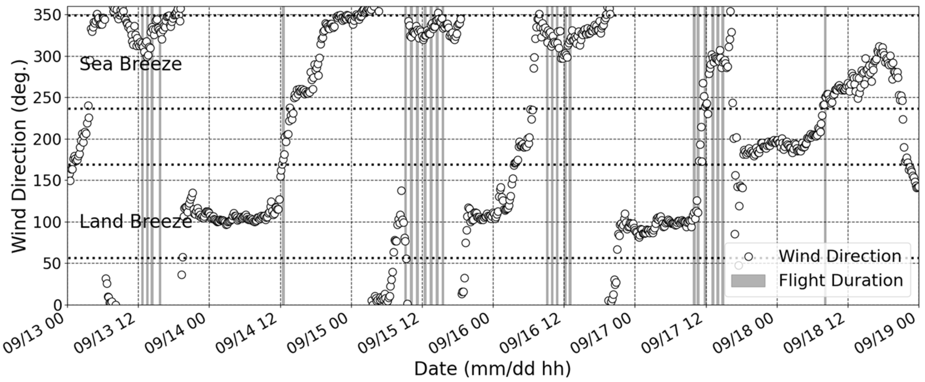
2.1. Study Area
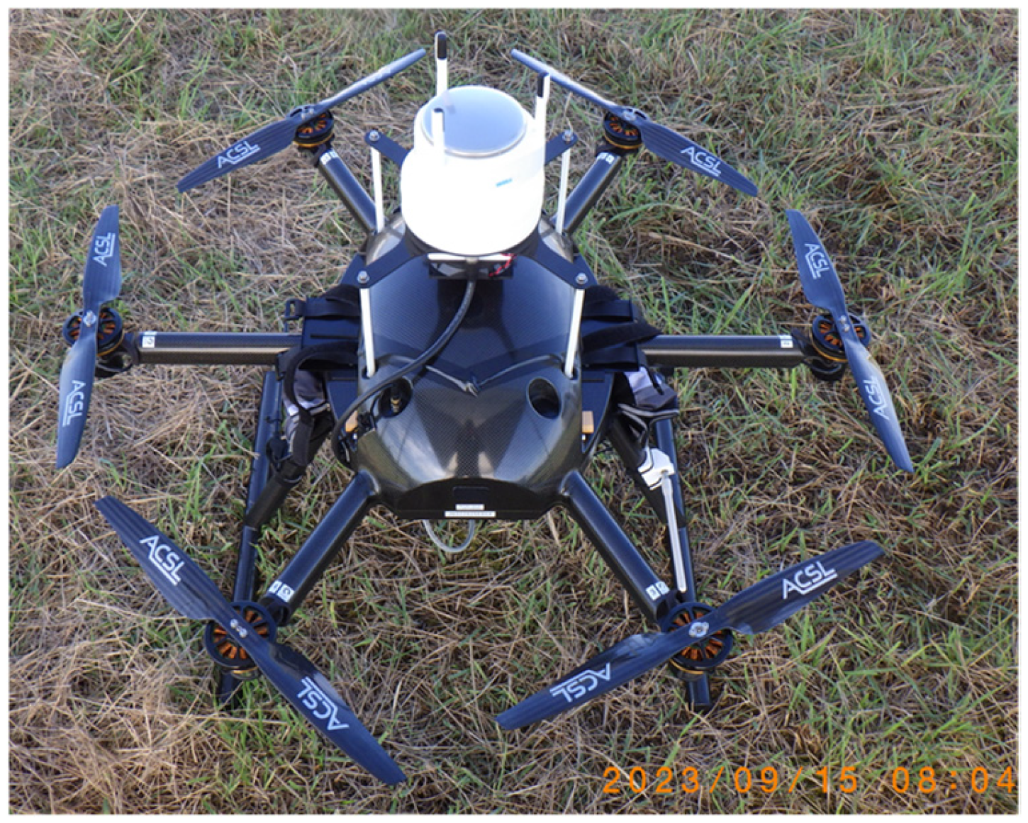
2.2. Equipment
2.3. Methodology
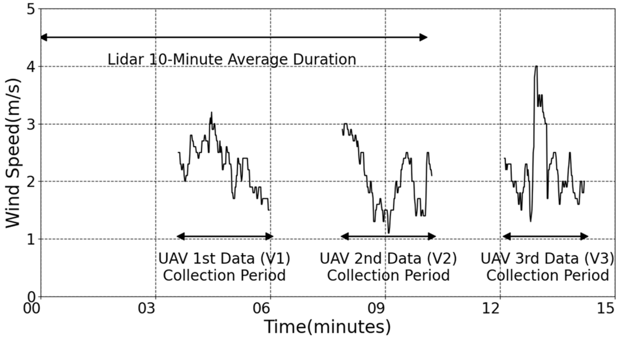
2.4. UAV Data Processing Techniques
3. Results
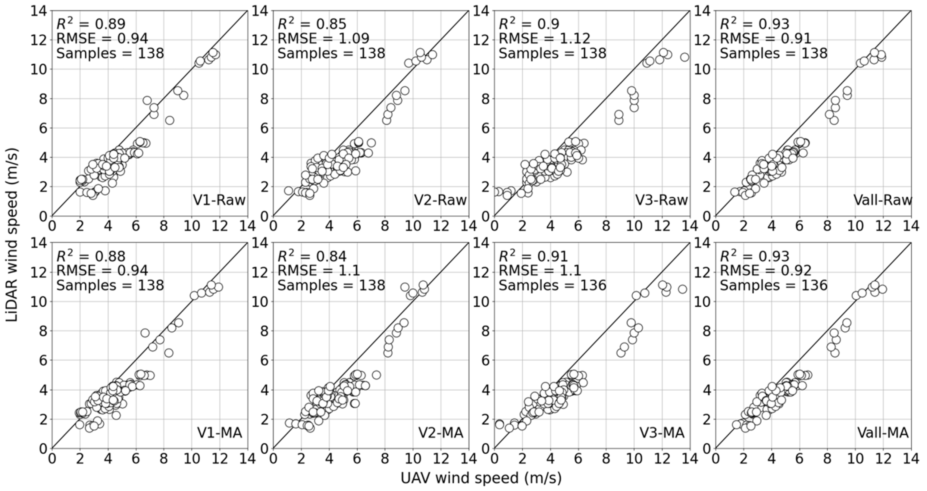
3.1. Analysis of UAV Data Processing
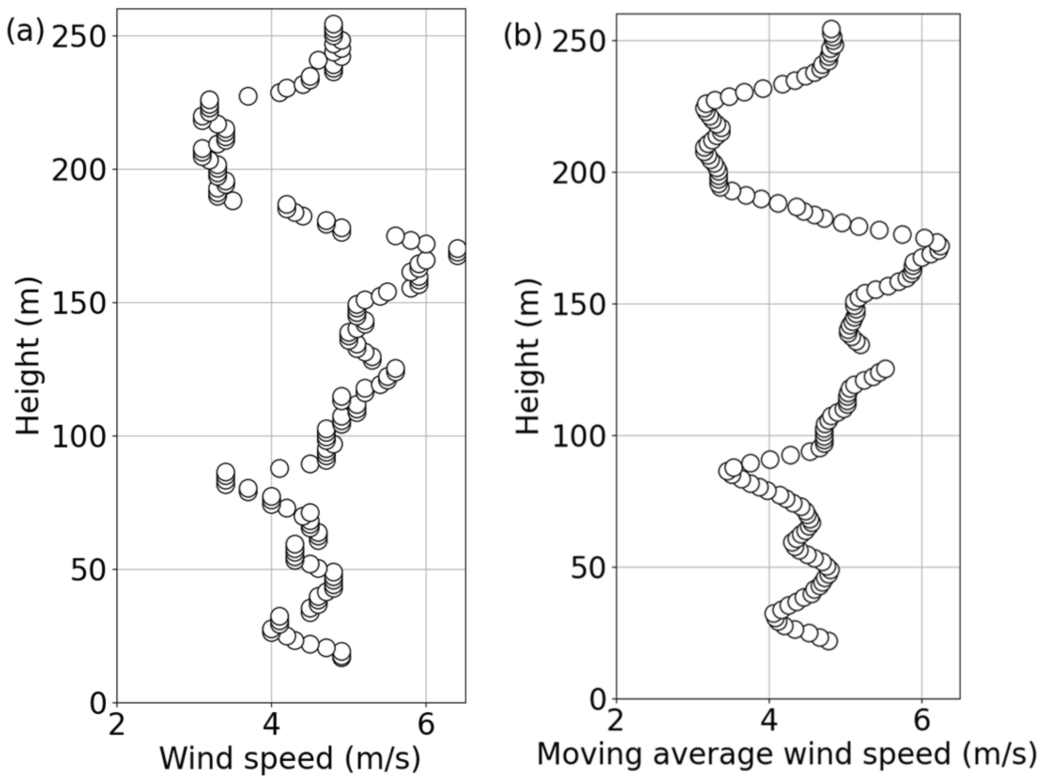
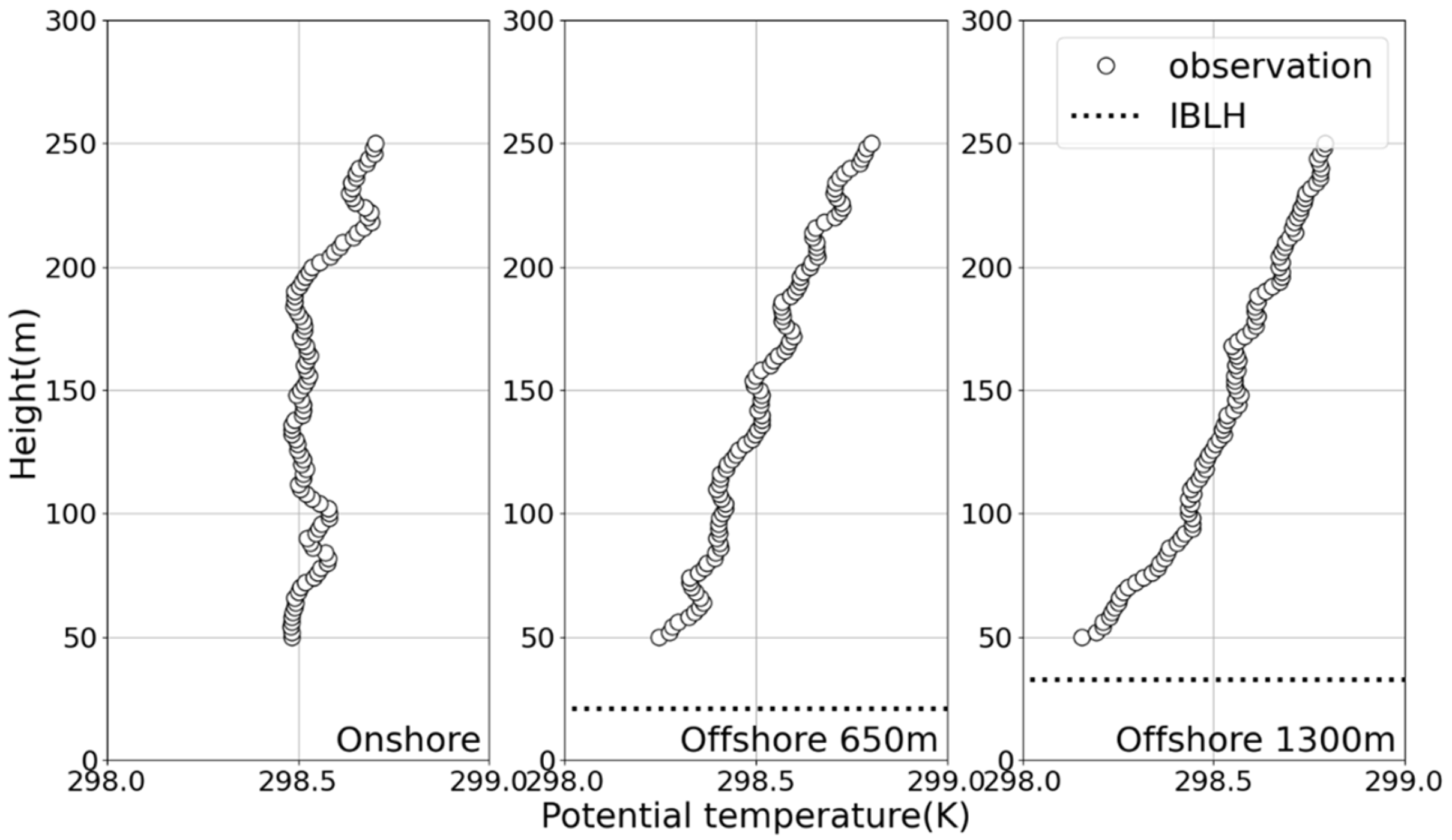
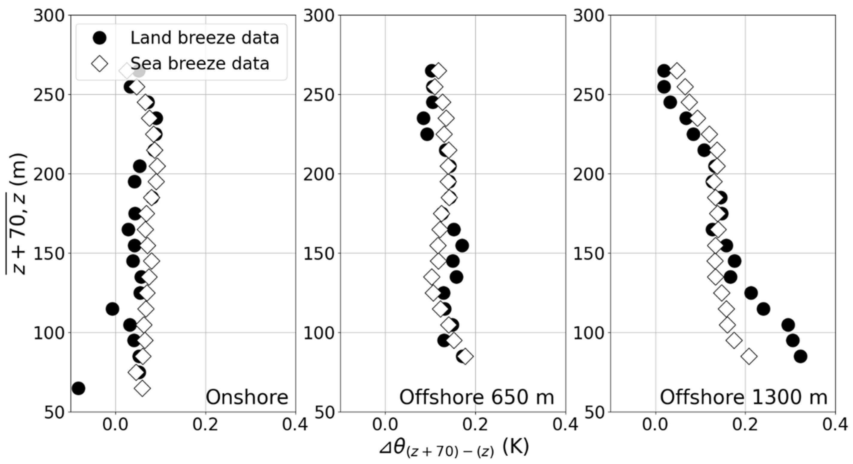
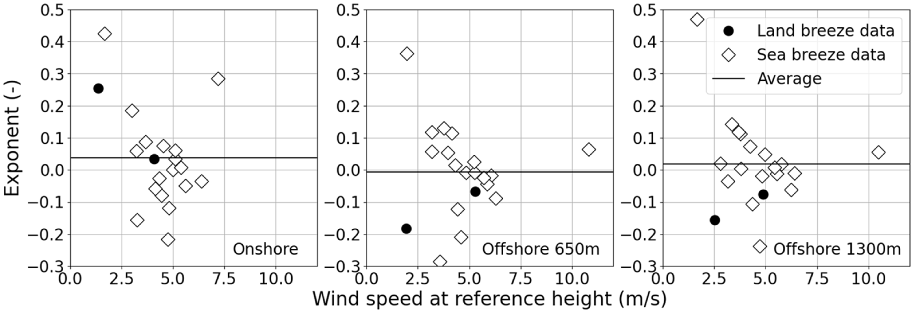
3.2. Vertical Atmospheric Structures in the Coastal Region of Japan
4. Discussion
Author Contributions
Funding
Data Availability Statement
Conflicts of Interest
References
- Wang, J.; Song, Y.; Liu, F.; Hou, R. Analysis and application of forecasting models in wind power integration: A review of multi-step-ahead wind speed forecasting models. Renew. Sustain. Energy Rev. 2016, 60, 960–981. [Google Scholar] [CrossRef]
- Yang, B.; Yu, T.; Shu, H.; Dong, J.; Jiang, L. Robust sliding-mode control of wind energy conversion systems for optimal power extraction via nonlinear perturbation observers. Appl. Energy 2018, 210, 711–723. [Google Scholar] [CrossRef]
- Holttinen, H.; Kiviluoma, J.; Forcione, A.; Milligan, M.; Smith, J.C.; Dobschinski, J.; van Roon, S.; Dillon, J.; Cutululis, N.; Orths, A.; et al. Design and Operation of Power Systems with Large Amounts of Wind Power; NREL/TP-5D00-66596; VTT Tiedotteita Valtion Teknillinen Tutkimuskeskus: Espoo, Finland; USDOE Office of Energy Efficiency and Renewable Energy (EERE), Wind and Water Technologies Office (EE-4W): Washington, DC, USA, 2009; Available online: https://iea-wind.org/wp-content/uploads/2021/08/T268.pdf (accessed on 3 December 2024).
- Schulz-Stellenfleth, J.; Emeis, S.; Dörenkämper, M.; Bange, J.; Cañadillas, B.; Neumann, T.; Schneemann, J.; Weber, I.; zum Berge, K.; Platis, A.; et al. Coastal impacts on offshore wind farms—A review focussing on the German Bight area. Meteorol. Z. 2022, 31, 289–315. [Google Scholar] [CrossRef]
- Archer, C.L.; Colle, B.A.; Delle Monache, L.; Dvorak, M.J.; Lundquist, J.; Bailey, B.H.; Beaucage, P.; Churchfield, M.J.; Fitch, A.C.; Kosovic, B.; et al. Meteorology for coastal/offshore wind energy in the United States: Recommendations and research needs for the next 10 years. Bull. Amer. Meteorol. Soc. 2014, 95, 515–519. [Google Scholar] [CrossRef]
- Hasager, C.; Stein, D.; Courtney, M.; Peña, A.; Mikkelsen, T.; Stickland, M.; Oldroyd, A. Hub height ocean winds over the North Sea observed by the NORSEWInD lidar array: Measuring techniques, quality control and data management. Remote Sens. 2013, 5, 4280–4303. [Google Scholar] [CrossRef]
- Clifton, A.; Clive, P.; Gottschall, J.; Schlipf, D.; Simley, E.; Simmons, L.; Stein, D.; Trabucchi, D.; Vasiljevic, N.; Würth, I. IEA wind Task 32: Wind lidar identifying and mitigating barriers to the adoption of wind lidar. Remote Sens. 2018, 10, 406. [Google Scholar] [CrossRef]
- Gottschall, J.; Wolken-Möhlmann, G.; Viergutz, T.; Lange, B. Results and conclusions of a floating-lidar offshore test. Energy Procedia 2014, 53, 156–161. [Google Scholar] [CrossRef]
- Rott, A.; Schneemann, J.; Theuer, F.; Trujillo Quintero, J.J.; Kühn, M. Alignment of scanning lidars in offshore wind farms. Wind Energy Sci. 2022, 7, 283–297. [Google Scholar] [CrossRef]
- Shimada, S.; Goit, J.P.; Ohsawa, T.; Kogaki, T.; Nakamura, S. Coastal wind measurements using a single scanning LiDAR. Remote Sens. 2020, 12, 1347. [Google Scholar] [CrossRef]
- Deutscher Wetterdienst (DWD). The FINO-WIND Project. Available online: https://www.dwd.de/EN/research/projects/fino_wind/fino_wind_en_node.html (accessed on 19 August 2024).
- Wagner, D.; Steinfeld, G.; Witha, B.; Wurps, H.; Reuder, J. Low level jets over the southern North Sea. Meteorol. Z. 2019, 28, 389–415. [Google Scholar] [CrossRef]
- Dörenkämper, M.; Optis, M.; Monahan, A.; Steinfeld, G. On the offshore advection of boundary-layer structures and the influence on offshore wind conditions. Bound. Layer Meteorol. 2015, 155, 459–482. [Google Scholar] [CrossRef]
- Gadde, S.N.; Stevens, R.J.A.M. Effect of low-level jet height on wind farm performance. J. Renew. Sustain. Energy 2021, 13, 013305. [Google Scholar] [CrossRef]
- Taylor, P.A. On wind and shear stress profiles above a change in surface roughness. Q. J. R. Meteorol. Soc. 1969, 95, 77–91. [Google Scholar] [CrossRef]
- Barthelmie, R.J.; Palutikof, J.P. Coastal wind speed modelling for wind energy applications. J. Wind Eng. Ind. Aerodyn. 1996, 62, 213–236. [Google Scholar] [CrossRef]
- Lange, B.; Larsen, S.; Højstrup, J.; Barthelmie, R. Importance of thermal effects and sea surface roughness for offshore wind resource assessment. J. Wind Eng. Ind. Aerodyn. 2004, 92, 959–988. [Google Scholar] [CrossRef]
- Emeis, S.; Harris, M.; Banta, R.M. Boundary-layer anemometry by optical remote sensing for wind energy applications. Meteorol. Z. 2007, 16, 337–347. [Google Scholar] [CrossRef]
- Konagaya, M.; Ohsawa, T.; Inoue, T.; Mito, T.; Kato, H.; Kawamoto, K. Land–sea contrast of nearshore wind conditions: Case study in Mutsu-Ogawara. Sola 2021, 17, 234–238. [Google Scholar] [CrossRef]
- Shimura, T.; Inoue, M.; Tsujimoto, H.; Sasaki, K.; Iguchi, M. Estimation of wind vector profile using a hexarotor unmanned aerial vehicle and its application to meteorological observation up to 1000 m above surface. J. Atmos. Ocean. Technol. 2018, 35, 1621–1631. [Google Scholar] [CrossRef]
- Sasaki, K.; Inoue, M.; Shimura, T.; Iguchi, M. In situ, rotor-based drone measurement of wind vector and aerosol concentration in volcanic areas. Atmosphere 2021, 12, 376. [Google Scholar] [CrossRef]
- Van der Hoven, I. Power spectrum of horizontal wind speed in the frequency range from 0.0007 to 900 cycles per hour. J. Meteorol. 1957, 14, 160–164. [Google Scholar] [CrossRef]
- Ministry of Economy, Trade and Industry. Available online: https://www.meti.go.jp/english/index.html (accessed on 19 August 2024).
- Debnath, M.; Doubrawa, P.; Optis, M.; Hawbecker, P.; Bodini, N. Extreme wind shear events in US offshore wind energy areas and the role of induced stratification. Wind Energy Sci. 2021, 6, 1043–1059. [Google Scholar] [CrossRef]
- Garratt, J.R. The Atmospheric Boundary Layer; Cambridge University Press: Cambridge, UK, 1992. [Google Scholar]


| Body and Attachments | Specifications |
|---|---|
| UAV body | Height: 536 mm Total weight: 7.1 kg Max payload: 2.75 kg Wind resistance: 10 m/s Battery: 12,000 mAh × 2 |
| Ultrasonic wind sensor | WXT532 made by Vaisala (Vantaa, Finland) Accuracy: ±3% (in 10 m/s) |
| Thermal sensor | NFR C3-0508-30 made by Netsushin (Saitama, Japan) Accuracy: ±0.3 K Forced ventilation and a filter covering the sensor to avoid direct solar radiation |
Disclaimer/Publisher’s Note: The statements, opinions and data contained in all publications are solely those of the individual author(s) and contributor(s) and not of MDPI and/or the editor(s). MDPI and/or the editor(s) disclaim responsibility for any injury to people or property resulting from any ideas, methods, instructions or products referred to in the content. |
© 2025 by the authors. Licensee MDPI, Basel, Switzerland. This article is an open access article distributed under the terms and conditions of the Creative Commons Attribution (CC BY) license (https://creativecommons.org/licenses/by/4.0/).
Share and Cite
Goto, K.; Uchida, T.; Kishida, T.; Nohara, D.; Nakao, K.; Sato, A. Investigating Coastal Effects on Offshore Wind Conditions in Japan Using Unmanned Aerial Vehicles. Energies 2025, 18, 1131. https://doi.org/10.3390/en18051131
Goto K, Uchida T, Kishida T, Nohara D, Nakao K, Sato A. Investigating Coastal Effects on Offshore Wind Conditions in Japan Using Unmanned Aerial Vehicles. Energies. 2025; 18(5):1131. https://doi.org/10.3390/en18051131
Chicago/Turabian StyleGoto, Kazutaka, Takanori Uchida, Takeshi Kishida, Daisuke Nohara, Keisuke Nakao, and Ayumu Sato. 2025. "Investigating Coastal Effects on Offshore Wind Conditions in Japan Using Unmanned Aerial Vehicles" Energies 18, no. 5: 1131. https://doi.org/10.3390/en18051131
APA StyleGoto, K., Uchida, T., Kishida, T., Nohara, D., Nakao, K., & Sato, A. (2025). Investigating Coastal Effects on Offshore Wind Conditions in Japan Using Unmanned Aerial Vehicles. Energies, 18(5), 1131. https://doi.org/10.3390/en18051131