Comparative Analysis of Offshore Wind Resources and Optimal Wind Speed Distribution Models in China and Europe

Abstract

Offshore wind resources in China and Europe are systematically compared, focusing on wind speed characteristics and the selection of optimal wind speed probability distribution models. Using 20 years of data at 10 m and 100 m above sea level, seven unimodal wind speed probability distribution models were applied. The results point out that China’s offshore wind resources exhibit high spatial and temporal variability, influenced by monsoons and typhoons, while European seas are characterized by stable wind patterns. Among the models tested, the Weibull distribution is the most accurate one for wind speed fitting, while the Generalized Extreme Value and Gamma models perform better in regions with higher skewness and extreme wind events. This study highlights the importance of wind speed characteristics, such as skewness and kurtosis, in selecting the optimal model. These findings provide valuable guidance for the improvement of offshore wind energy assessments and the selection of appropriate models. Future research should explore advanced techniques, such as machine learning and hybrid models, to better capture complex wind patterns and enhance model accuracy.

1. Introduction

Wind energy has emerged as one of the most promising renewable energy sources in the global transition toward sustainable energy [1,2,3,4]. Offshore wind energy is particularly valuable due to its higher, more stable wind speeds and consistent patterns, which reduce turbulence and offer greater energy potential compared to onshore sites [5]. These advantages make offshore wind farms central to the decarbonization of the energy sector [1,6,7,8,9]. As nations strive to meet renewable energy targets, offshore wind resource development has become a critical focus, with substantial investments in this sector globally [6,7,8,10,11,12,13,14].

However, accurately assessing offshore wind resources is challenging due to the complex and dynamic nature of wind patterns in coastal and offshore areas [15,16]. These regions exhibit significant temporal and spatial variability, influenced by factors such as geographical location, seasonal shifts, and large-scale weather systems like monsoons or jet streams [1,11,12,17]. To address these challenges, wind speed probability distribution (WSPD) models have become a widely used approach for assessing wind resources over a given area [18]. Compared to time-series methods [19,20], these statistical models describe wind speed distributions using a set of parameters, offering an efficient and distinct approach. While wind direction also influences wind resource assessment [21,22,23,24], this study focuses solely on the statistical modeling of wind speed distributions.

WSPD models are generally classified into parametric models (e.g., Weibull [25], Gamma distributions [26], and mixtures of these distributions to describe the wind speed with bimodal or multimodal characteristics [27,28]) and non-parametric models (e.g., Kernel Density Estimation (KDE) [29,30] and Maximum Entropy Principle (MEP) [31,32]). Parametric models describe wind speed characteristics by estimating a set of parameters. These models are typically favored due to their good adaptability and computational efficiency, particularly in situations where data are limited or when conducting wind resource predictions in specific regions [33,34]. In contrast, non-parametric models are more flexible as they make no assumptions about the underlying distribution, but they also present certain challenges. For instance, KDE models often struggle with bandwidth selection, where improper choices can lead to overfitting or underfitting, compromising accuracy [35]. Similarly, the Maximum Entropy Principle (MEP) faces challenges in constraint selection, with inappropriate constraints potentially yielding unstable or implausible solutions [32]. Therefore, parametric models are more suitable for large-scale applications, such as offshore wind resource assessments.

In the field of parametric models for WSPD, previous studies primarily focus on onshore sites or region-specific wind resource assessments, as well as testing newly proposed WSPD models [33,36,37]. For example, ref. [37] assessed the Weibull distribution at three different turbine locations. The study found that for higher probabilities of null wind, the three-parameter Weibull distribution performed better than the two-parameter version. In addition, using five years of day-average wind speed data from 698 onshore wind stations in China, ref. [30] concluded that the generalized gamma and generalized extreme value distributions were better suited for fitting the WSPD in parametric models. Furthermore, based on five years of ERA-Interim reanalysis data at a height of 10 m, ref. [27] analyzed grid cells within exclusive economic zones (EEZs) to identify the best WSPD models across different countries worldwide. These studies suggest a deeper exploration of the relationship between WSPD models and wind characteristics.

Therefore, this study compares the performances of widely used WSPD models across diverse offshore regions, particularly in areas with distinct geographical and meteorological characteristics. The focus is on China and Europe to explore their applicability and limitations. Additionally, the study assesses how well these models capture the temporal and spatial variability in wind resources and how they account for regional factors like seasonal changes and extreme wind events. Using a 20-year wind speed dataset from both regions at two different heights, model performances are evaluated using metrics like R², RMSE, AIC, and BIC. Several machine learning methods are also employed to determine the importance of key wind characteristics. The goal is to provide recommendations for selecting the most suitable WSPD model for offshore wind resource assessments.

This paper is organized as follows: Section 2 presents the materials and methods, including data resources and quality assessment (Section 2.1), the analysis of wind resource characteristics (Section 2.2), and the wind speed modeling approach (Section 2.3). Section 3 presents the comparison of offshore wind resources between China and Europe (Section 3.1); meanwhile, the model performance evaluation (Section 3.2), the distribution of optimal and suboptimal models (Section 3.3), and guidelines for model selection (Section 3.4) are also analyzed. Finally, Section 4 gives the concluding remarks and suggests directions for future research.

2. Materials and Methods

2.1. Data Resources and Quality Assessment

Released in 2019, ERA5 is the fifth-generation global atmospheric reanalysis produced by the European Centre for Medium-Range Weather Forecasts (ECMWF), covering data from 1950 to the present. ECMWF has rigorously ensured the quality and control of the ERA5 datasets, making them highly reliable for various applications [38]. ERA5 offers superior temporal (1 h) and spatial resolution (0.25° × 0.25°, ~31 km) compared to reanalysis products like MERRA-2 and JRA-55 [39]. Although its accuracy decreases slightly in coastal areas due to land–sea interactions, ERA5 performs better in oceanic regions and is highly effective for assessing wind energy, particularly over flat, homogeneous terrains [15,40,41]. Thus, despite these minor limitations, ERA5 is widely accepted as a reliable data source for offshore studies [41,42,43,44,45,46,47].

This study focuses on wind data from two representative offshore regions: Europe and China. The hourly u- and v-components of wind data at 10 m and 100 m heights from ERA5 datasets were utilized to calculate wind speed and wind direction. The data span from 00:00 UTC on 1 January 2004 to 23:00 UTC on 31 December 2023, which covered the area from 45° N to 75° N and −30° E to 30° E for Europe and from 15° N to 42° N and 105° E to 130° E for China. Specifically, the calculation period for seasonal distribution is from 00:00 UTC on 1 March 2004 to 23:00 UTC on 29 February 2024.

2.2. Wind Resource Characteristics Analysis

2.2.1. Data Preprocessing for Offshore Wind Resource Analysis

The wind speed V_i can be obtained according to the equation:

$$V_{\mathrm{i}}=\sqrt{u_{\mathrm{i}}^2+v_{\mathrm{i}}^2},$$

(1)

where u_i is the northward wind speed component. v_i is the eastward wind speed component.

The wind direction is mainly computed by the atan2d function [48], which can provide four-quadrant inverse tangent in degrees:

$$\mathrm{a}\mathrm{t}\mathrm{a}\mathrm{n}2(v_{\mathrm{i}},u_{\mathrm{i}})=\left\{\begin{array}{c}\begin{array}{cc}\mathrm{a}\mathrm{r}\mathrm{c}\mathrm{t}\mathrm{a}\mathrm{n}\left({\displaystyle \frac{v_{\mathrm{i}}}{u_{\mathrm{i}}}}\right),& u_{\mathrm{i}}>0;\end{array}\\ \begin{array}{cc}\mathrm{a}\mathrm{r}\mathrm{c}\mathrm{t}\mathrm{a}\mathrm{n}\left({\displaystyle \frac{v_{\mathrm{i}}}{u_{\mathrm{i}}}}\right)+\mathsf{\pi },& v_{\mathrm{i}}\ge 0,u_{\mathrm{i}}<0;\end{array}\\ \begin{array}{cc}\mathrm{a}\mathrm{r}\mathrm{c}\mathrm{t}\mathrm{a}\mathrm{n}\left({\displaystyle \frac{v_{\mathrm{i}}}{u_{\mathrm{i}}}}\right)-\mathsf{\pi },& v_{\mathrm{i}}<0,u_{\mathrm{i}}<0;\end{array}\\ \begin{array}{cc}+{\displaystyle \frac{\mathsf{\pi }}{2}},& v_{\mathrm{i}}>0,u_{\mathrm{i}}=0;\end{array}\\ \begin{array}{cc}-{\displaystyle \frac{\mathsf{\pi }}{2}},& v_{\mathrm{i}}<0,u_{\mathrm{i}}=0;\end{array}\\ \begin{array}{cc}\mathrm{u}\mathrm{n}\mathrm{d}\mathrm{e}\mathrm{f}\mathrm{i}\mathrm{n}\mathrm{e}\mathrm{d},& v_{\mathrm{i}}=0,u_{\mathrm{i}}=0,\end{array}\end{array}\right.$$

(2)

$$\mathrm{a}\mathrm{t}\mathrm{a}\mathrm{n}2\mathrm{d}(v_{\mathrm{i}},u_{\mathrm{i}})={\displaystyle \frac{180°}{\mathsf{\pi }}}·\mathrm{a}\mathrm{t}\mathrm{a}\mathrm{n}2(v_{\mathrm{i}},u_{\mathrm{i}}).$$

(3)

This function returns the angle in degrees between the positive x-axis (east) and the vector (u_i, v_i). The result ranges from −180 to 180 degrees. Subtracting the angle from 270 degrees converts the angle to be measured from the north (0 degrees), which aligns with the meteorological community. As a result, the northern, eastern, southern, and western directions are 0, 90, 180, and 270 degrees.

In this study, we employed a mask technique to the ERA5 reanalysis datasets to isolate marine regions. Therefore, only sea areas are analyzed, and land areas are excluded. The ‘global_land_mask’ library was employed to create the mask based on high-resolution topographic data [49,50]. Thereafter, marine areas were analyzed to ascertain the maximum, mean, and minimum wind parameters. The results are presented in Appendix A.

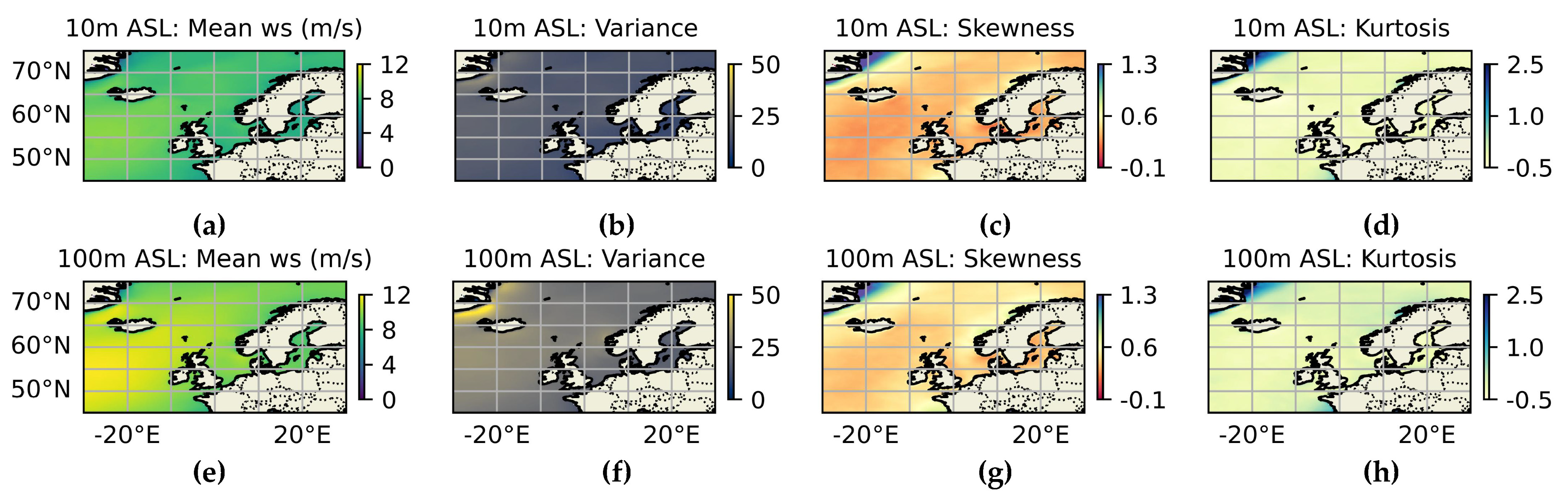
2.2.2. Statistical Characteristics of Wind Speed

In this section, we evaluate the wind speed characteristics through statistical analysis methods to reveal the variability and probability distribution patterns of the wind speed. In many regions, wind speed distributions deviate from a Gaussian (normal) distribution due to complex atmospheric and geographic factors, resulting in non-Gaussian wind fields in terms of asymmetry, extreme values, or multimodal distributions [27,28,51]. These statistical characteristics are essential for subsequent wind resource assessment and the selection of WSPD models. The analysis primarily includes the mean (μ), variance (σ²), skewness (S), and kurtosis (K) of the wind speed, which corresponds to the first fourth-order statistical moments, respectively [52]. The mean represents the central tendency of the wind speed, while variance measures its dispersion. Skewness describes the asymmetry in the wind speed distribution, with positive skewness indicating a right-skewed distribution and negative skewness indicating a left-skewed one. Kurtosis quantifies the sharpness of the distribution, where values greater than 3 indicate a sharper (leptokurtic) distribution and values less than 3 indicate a flatter (platykurtic) one. The specific methods and processes are detailed below, utilizing functions such as ‘scipy.stats.skew’ and related tools [1,53].

$$\left\{\begin{array}{l}\mu ={\displaystyle \frac{1}{N}}{\displaystyle \sum _{i=1}^N}{V}_{\mathrm{i}},\\ \begin{array}{c}{\sigma }^2={\displaystyle \frac{1}{N}}{\displaystyle \sum _{i=1}^N}{\left(V_{\mathrm{i}}-\mu \right)}^2,\\ S={\displaystyle \frac{\frac{1}{N}\sum _{i=1}^N{\left(V_{\mathrm{i}}-\mu \right)}^3}{{\sigma }^3}},\\ K={\displaystyle \frac{\frac{1}{N}\sum _{i=1}^{\mathrm{N}}{\left(V_{\mathrm{i}}-\mu \right)}^4}{{\sigma }^4}}.\end{array}\end{array}\right.$$

(4)

where V_i is the wind speed (m/s) at each time step and N is the total number of samples.

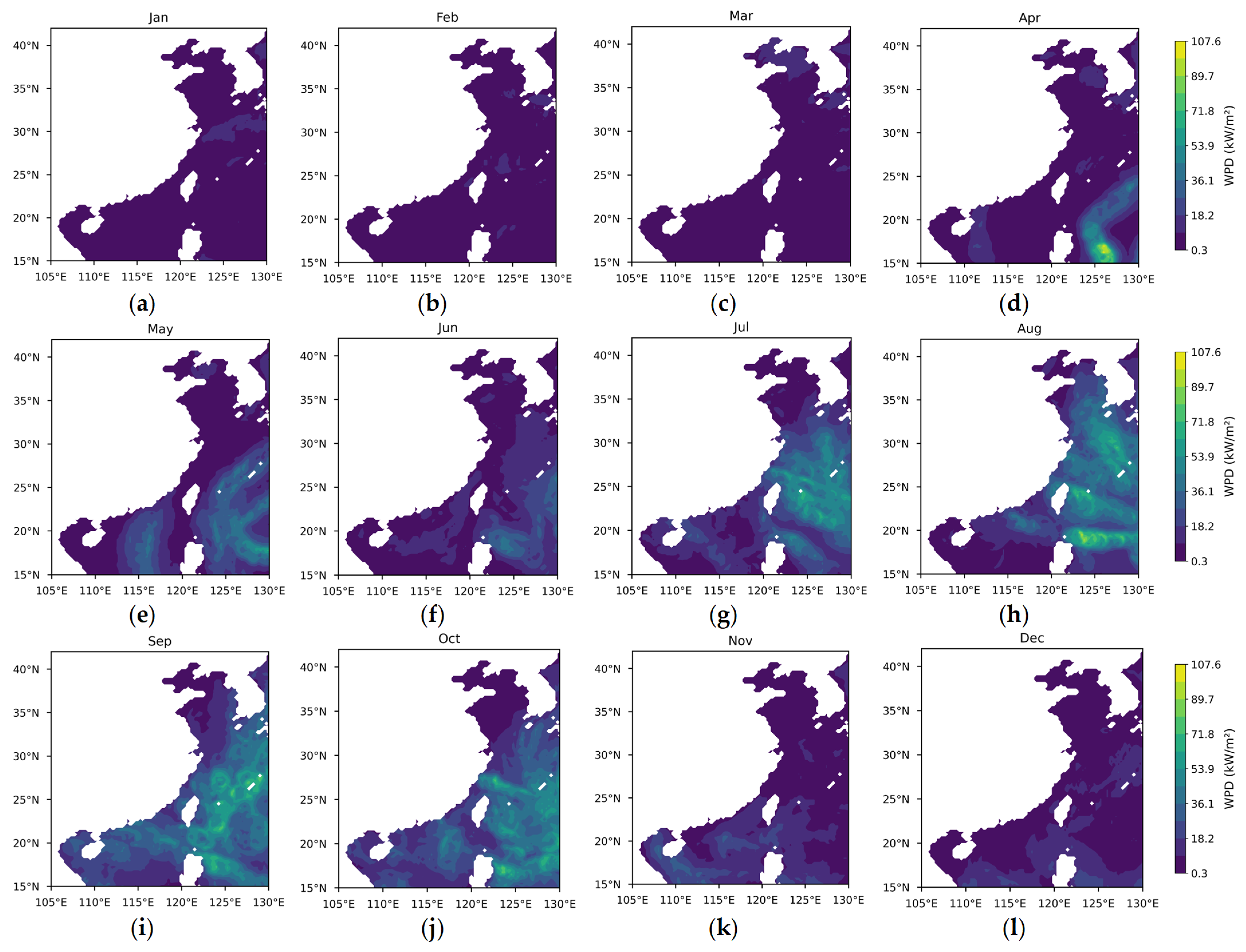
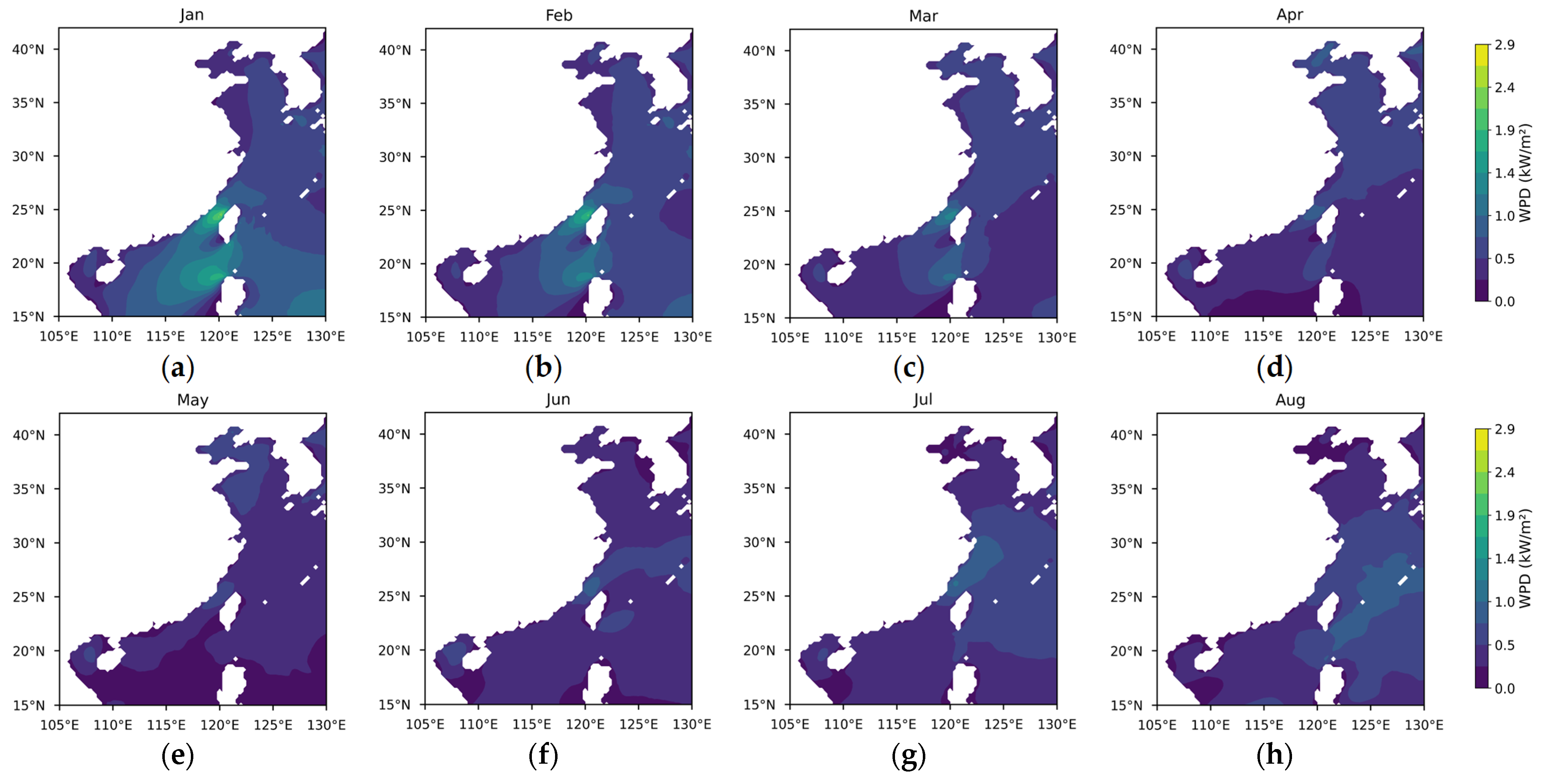
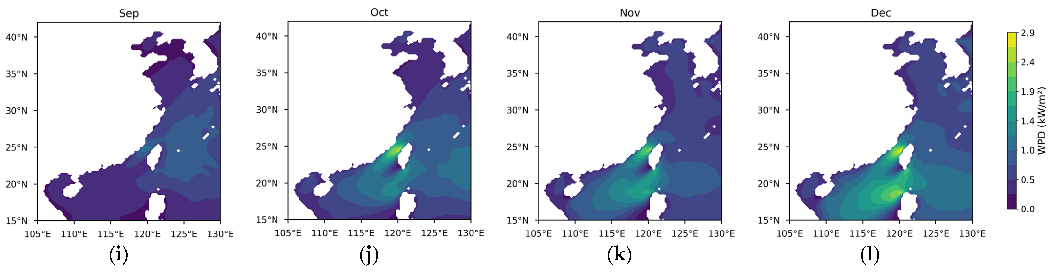
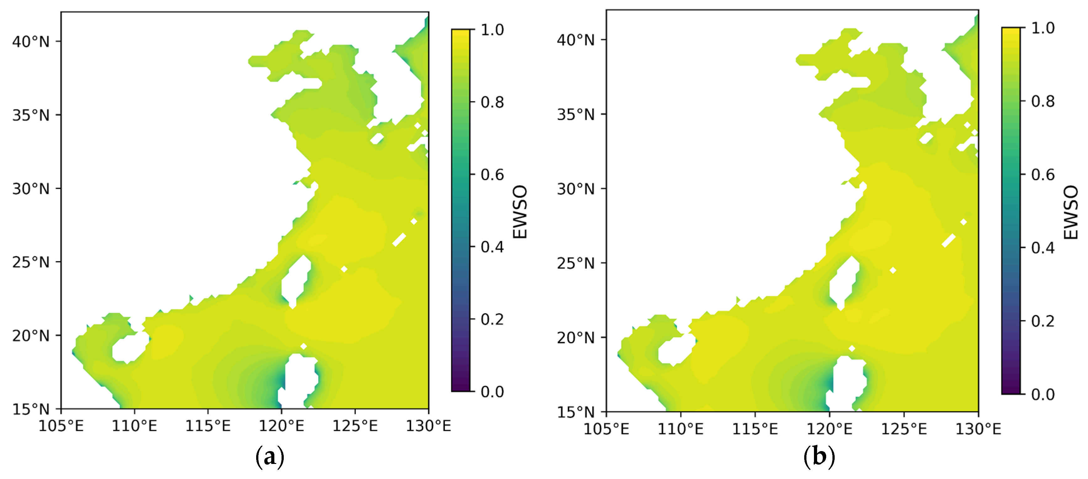
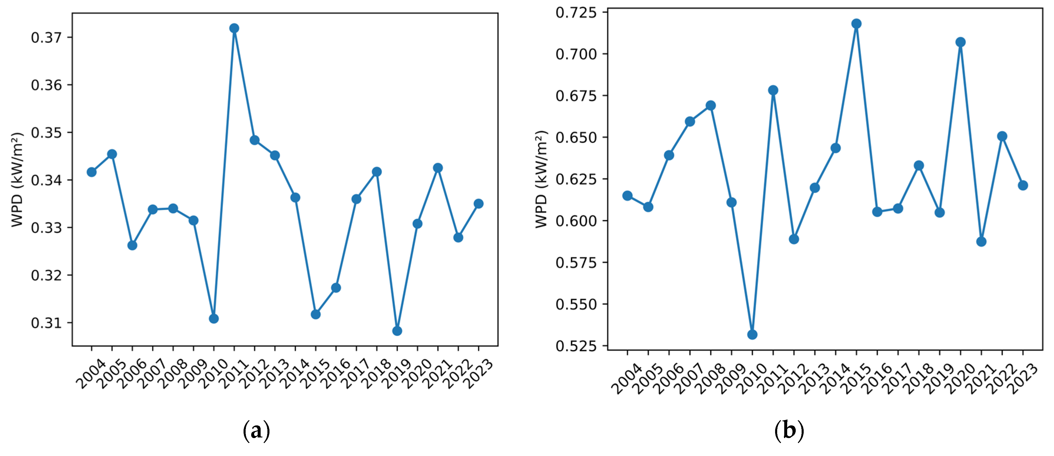
2.2.3. Theoretical Potential of Wind Resources

• Wind power density (WPD).

WPD represents the kinetic energy of the air passing through a unit cross-sectional area perpendicular to the airflow per unit time. This is a critical metric used to quantify the amount of energy available in the wind at a particular location. It can be measured in watts per square meter (W/m²) and calculated using the following formula [54,55]:

$$\mathrm{W}\mathrm{P}\mathrm{D}={\displaystyle \frac{1}{2}}\rho V_{\mathrm{i}}^3,$$

(5)

where ρ is the air density (kg/m³), typically assumed to be 1.225 kg/m³ at sea level under standard conditions.

Based on the wind power density formula, the hourly wind power density from 2004 to 2023 was calculated, and the multiyear averages for annual, seasonal, and monthly data were derived. For clarity, the unit of WPD was kilowatts per square meter (kW/m²).

2.

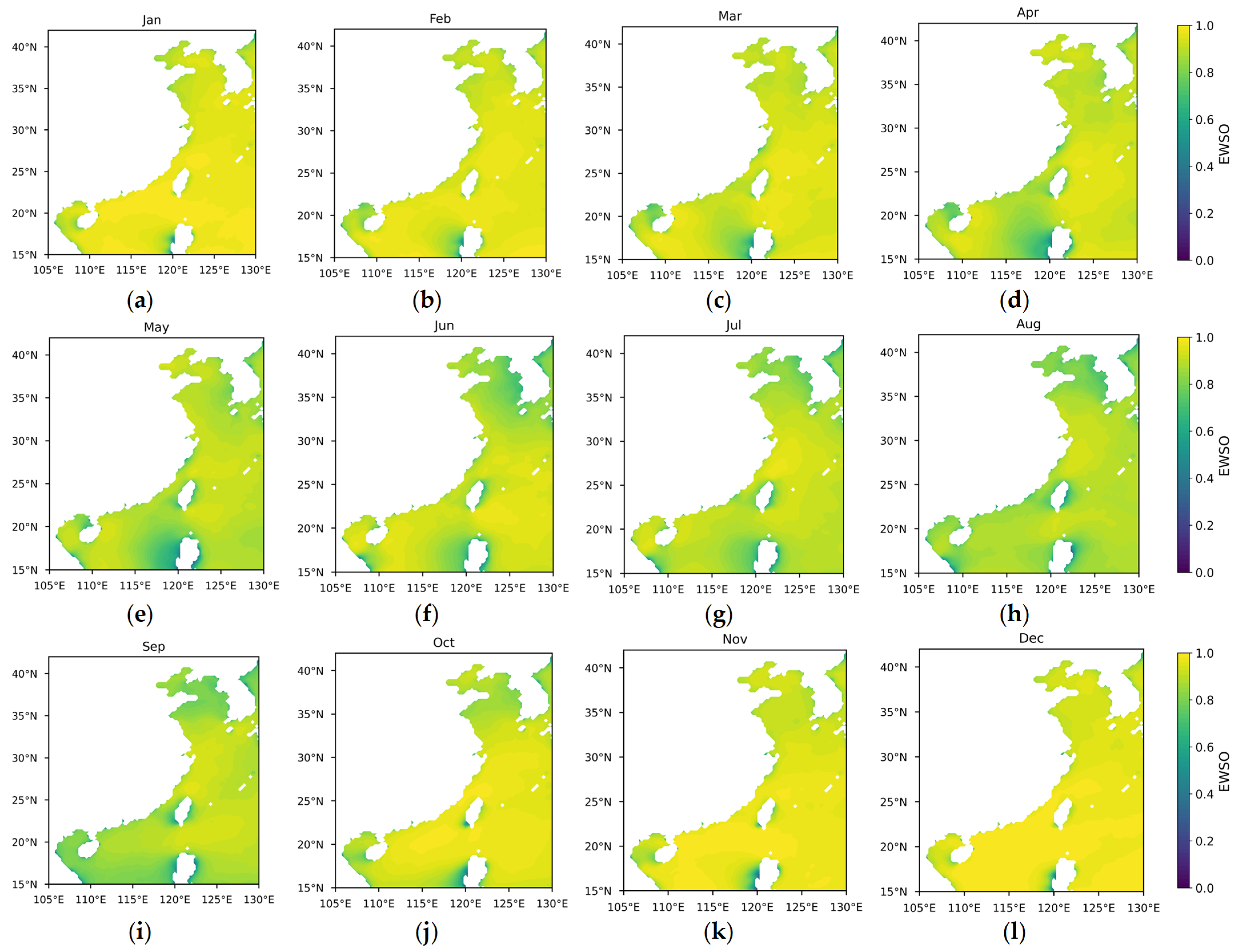
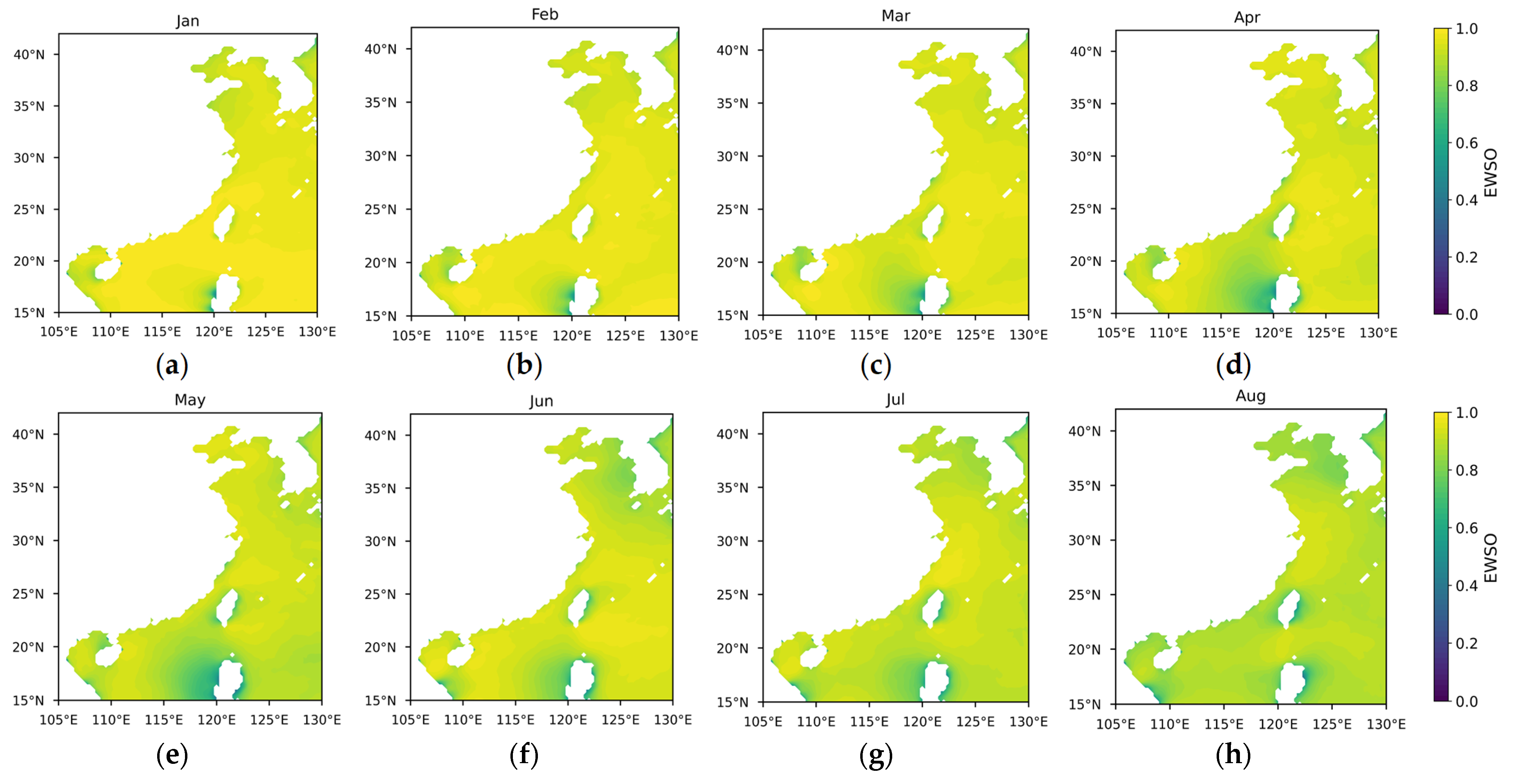
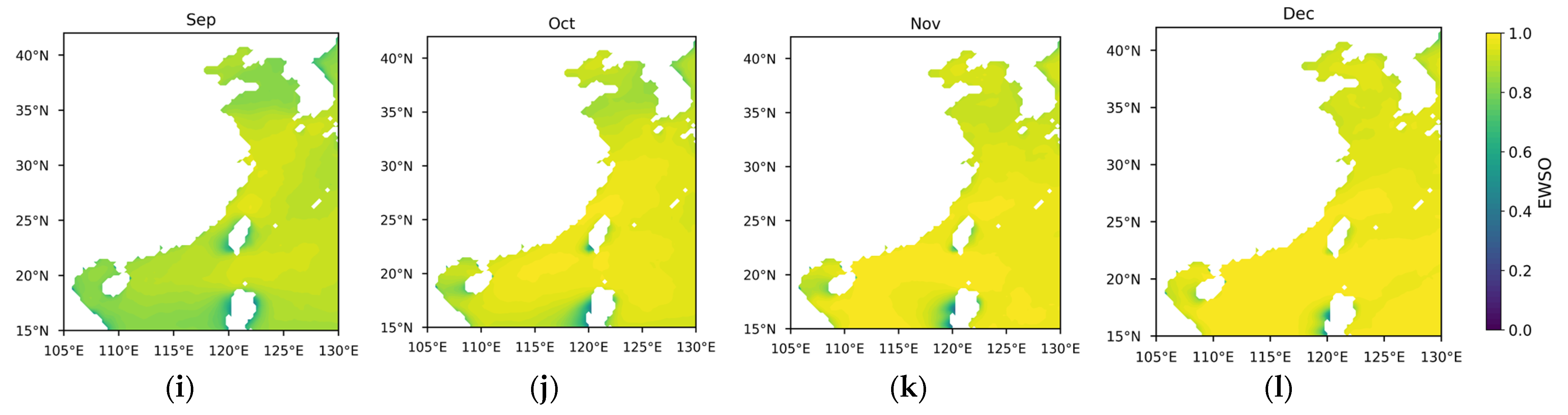
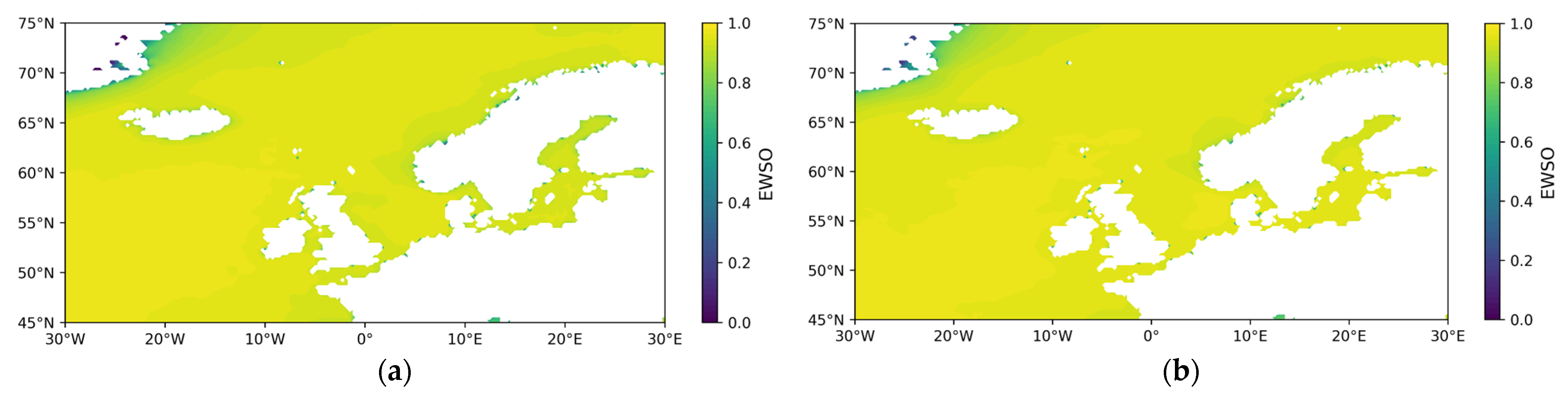
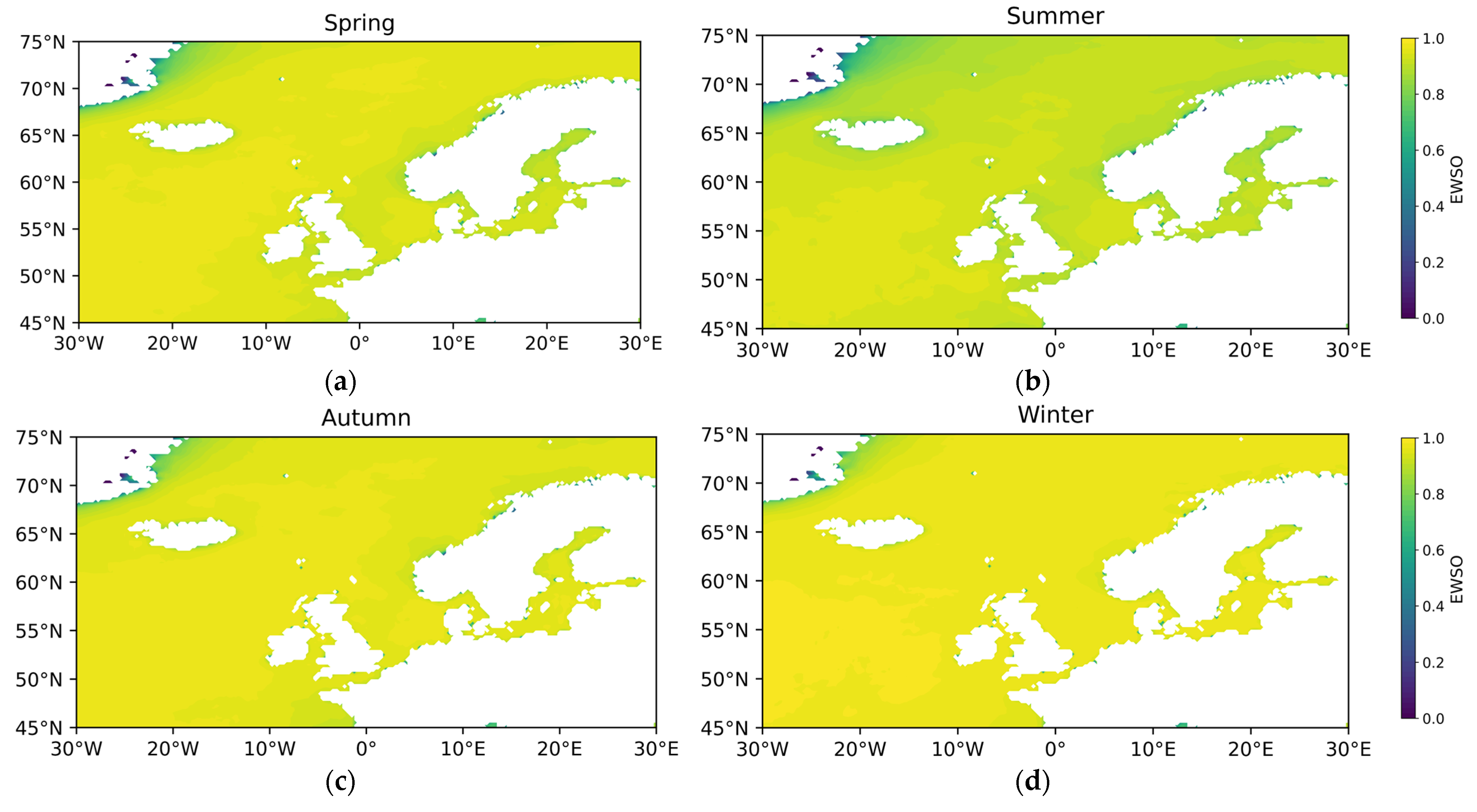
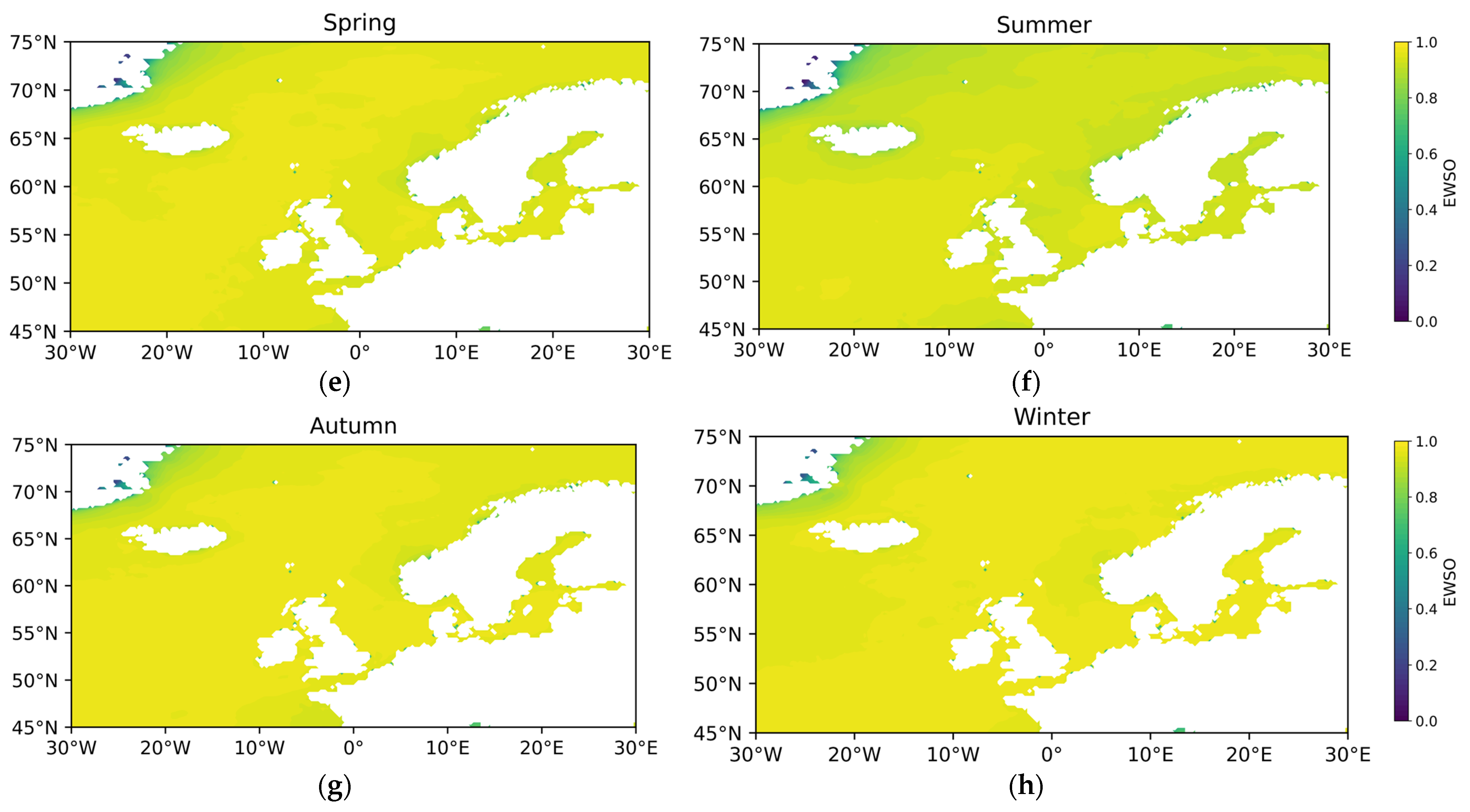
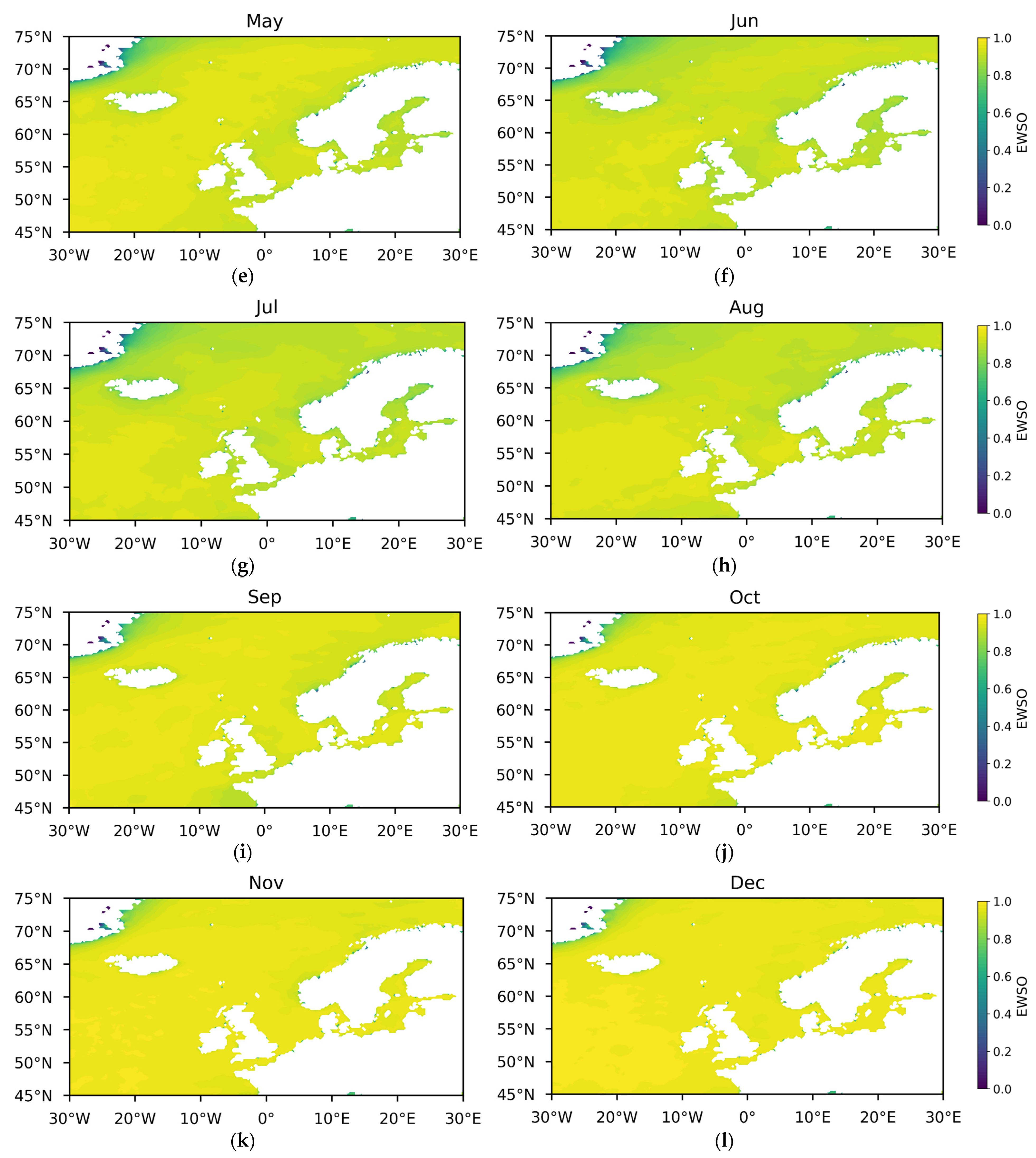
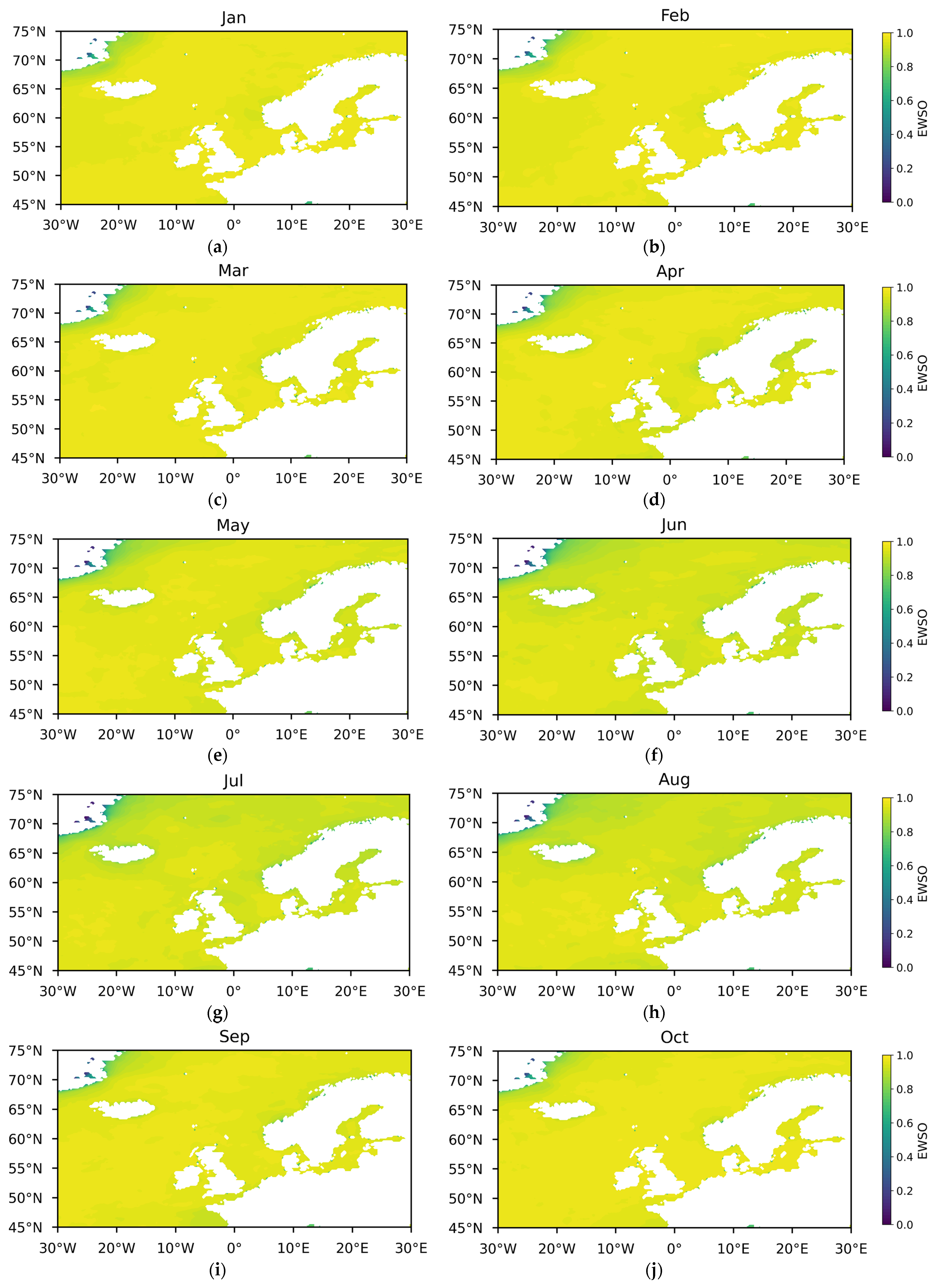
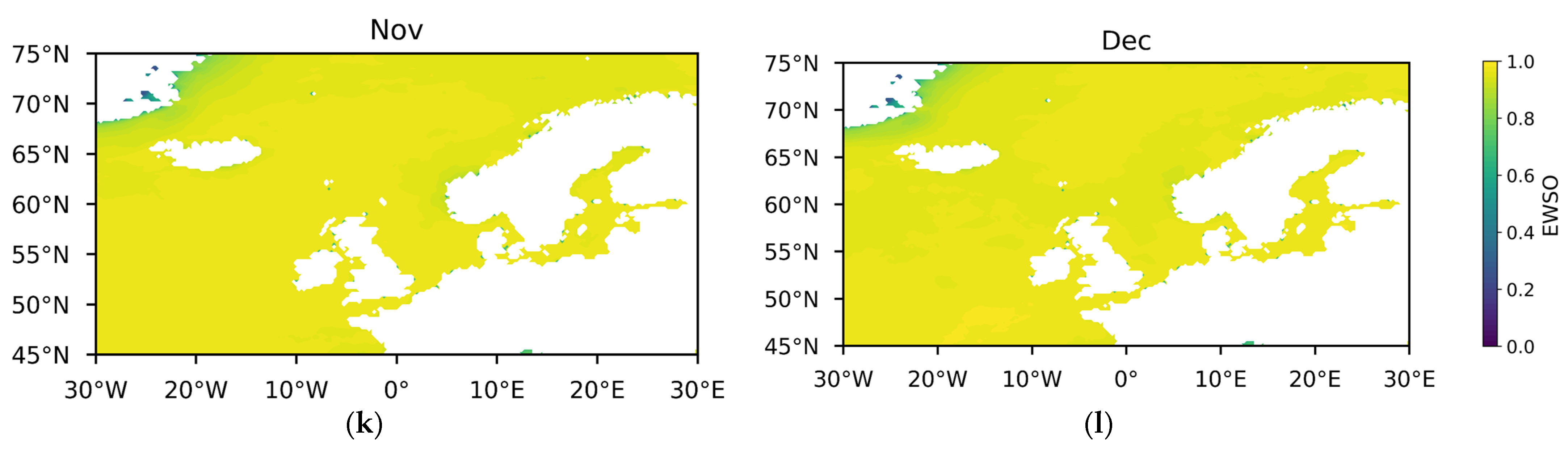
Effective wind speed occurrence (EWSO).

EWSO is a metric to assess the availability and usability of wind resources at a specific site. This measure characterizes the range of wind speeds that are sufficient to generate power from a wind turbine, specifically between the turbine’s cut-in and cut-out speeds. EWSO is quantified as the percentage of time during which the wind speed at a given location remains within this effective operational range [55]:

$$\mathrm{E}\mathrm{W}\mathrm{S}\mathrm{O}={\displaystyle \frac{t_{\mathrm{n}}}{T_{\mathrm{n}}}}\times 100\mathrm{\%}.$$

(6)

where t_n is the number of hours during which the wind speed falls within the turbine’s operational range; here, we adopted 3 m/s (cut-in) to 25 m/s (cut-out). T_n is the total number of hours in the period of interest.

2.2.4. Stability Assessment of Wind Resources

• Coefficient of variation (CV).

The CV is a statistical measure to evaluate the stability and consistency of wind speeds over a specified time period. The coefficient of variation (CV) is defined as the ratio of the standard deviation to the mean of the wind speed and is typically expressed as a percentage. A lower CV indicates greater consistency and stability in wind speeds, which is conducive to wind energy generation as it reduces the variability in power output [56,57]:

$$\mathrm{C}\mathrm{V}={\displaystyle \frac{{\sigma }_{\mathrm{P}}}{P_{\mathrm{a}\mathrm{v}\mathrm{e}}}},$$

(7)

where σ_P is the standard deviation of WPD and P_ave is the mean value of WPD.

2.

Monthly variability index (MVI).

In order to illustrate the inter-monthly differences in wind resources, the MVI of the wind power density was calculated. A high MVI value denotes a more pronounced inter-monthly variability, which is less conducive to wind energy development. Conversely, a low MVI value indicates a reduction in variability, thereby creating a more productive environment for wind energy utilization. The MVI can be calculated as [57,58]:

$$\mathrm{M}\mathrm{V}\mathrm{I}={\displaystyle \frac{P_{\mathrm{M}1}-P_{\mathrm{M}12}}{P_{\mathrm{y}\mathrm{e}\mathrm{a}\mathrm{r}}}},$$

(8)

where P_M1 and P_M12 are the highest and lowest monthly means of WPD. P_year is the annual mean wind power density.

3.

Seasonal variability index (SVI).

Similarly, the SVI was employed for the purpose of quantifying the seasonal fluctuations in wind resources in a manner analogous to the approach for the MVI. It promotes the comprehension of the seasonal patterns throughout the year. The SVI can be calculated as follows:

$$\mathrm{S}\mathrm{V}\mathrm{I}={\displaystyle \frac{P_{\mathrm{S}1}-P_{\mathrm{S}4}}{P_{\mathrm{y}\mathrm{e}\mathrm{a}\mathrm{r}}}}.$$

(9)

where P_S1 and P_S4 are the highest and lowest seasonal means of the WPD.

2.3. WSPD-Based Wind Speed Modeling

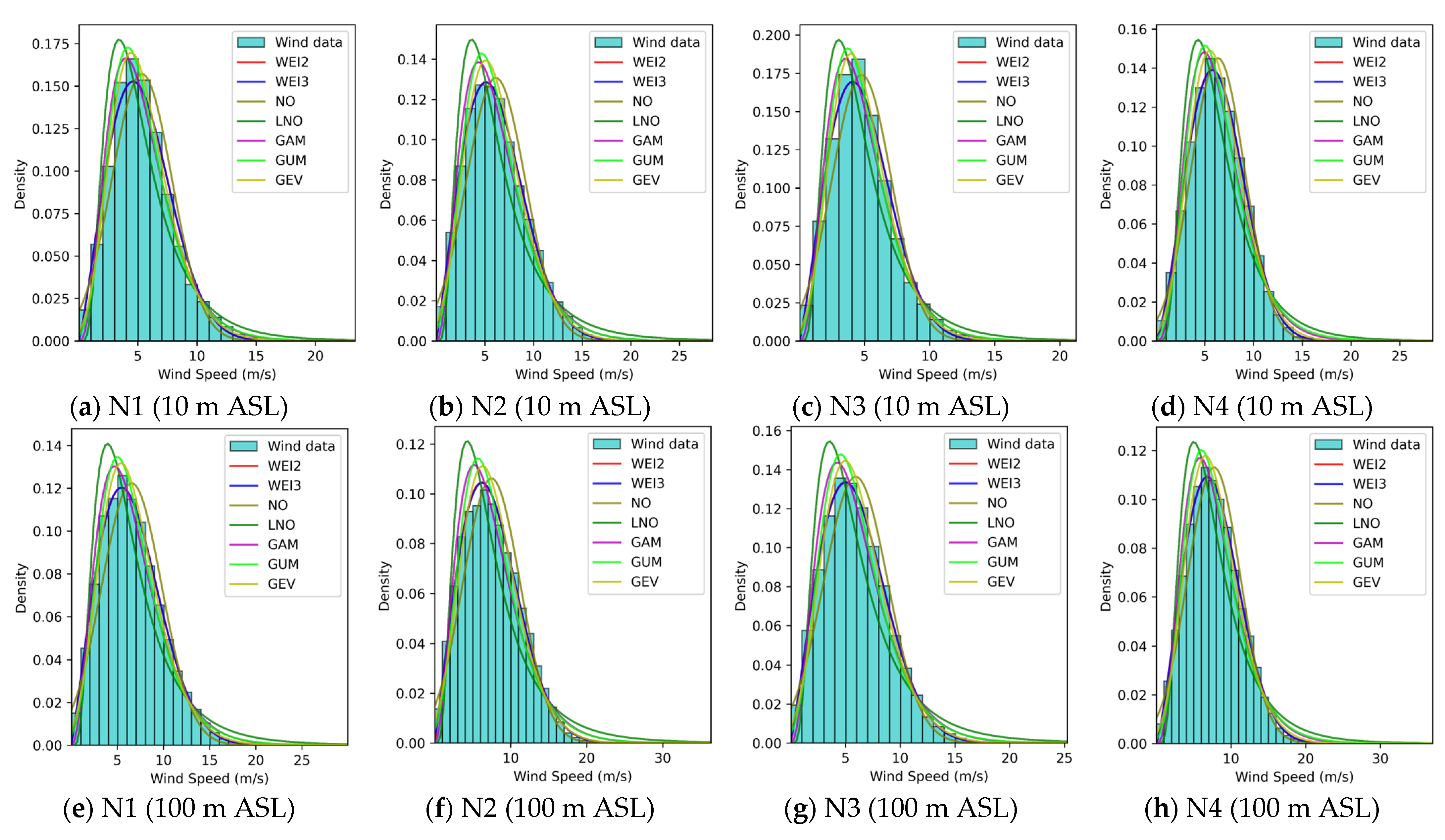
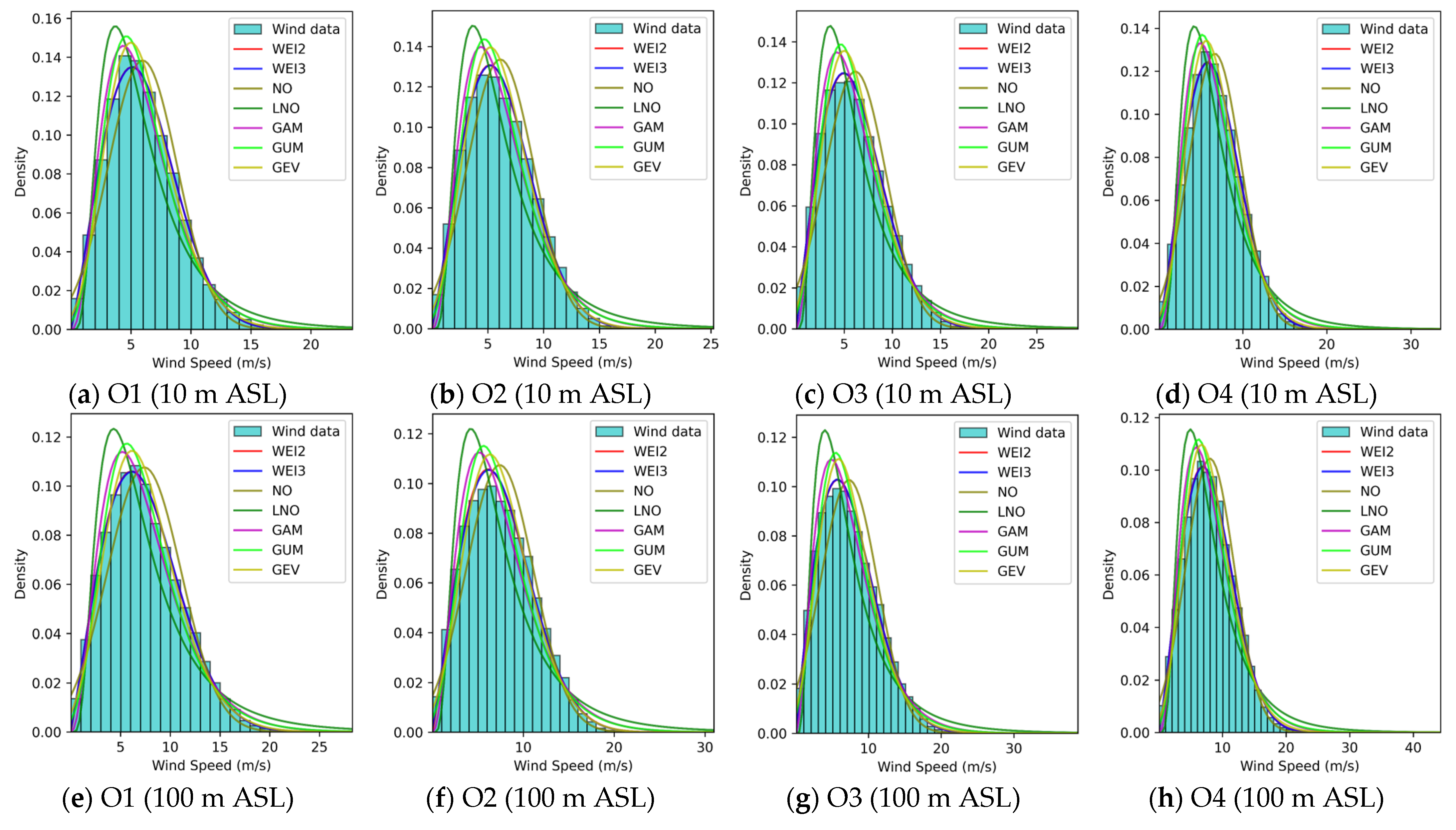
2.3.1. Selection of WSPD Models

In this section, we present the selection of the wind speed probability distribution (WSPD) models used to model the wind speed characteristics in the study area. Choosing an appropriate model is crucial for the accurate evaluation of wind speed properties, such as its mean, variance, skewness, and kurtosis. Given the broad temporal and spatial range of the study area, we focused on some popular unimodal, non-mixture models for initial modeling. This choice was based on the need for a comparison among simple models to understand wind speed distributions. Additionally, unimodal distributions are computationally effective and compatible with large datasets, especially in areas with significant spatial and temporal variability.

In this study, the probability distribution function (pdf) models listed in

Table 1. Selected unimodal WSPD models.

Name (Symbol)	Np	Probability Distribution Function	Key Features	Chosen Reasons
Weibull (WEI2)	2	$f\left(V_i;\alpha ,k\right)={\displaystyle \frac{k}{\alpha }}{\left({\displaystyle \frac{V_i}{\alpha }}\right)}^{k-1}\mathrm{e}\mathrm{x}\mathrm{p}\left(-{\left({\displaystyle \frac{V_i}{\alpha }}\right)}^k\right)$	Suitable for most wind speed distributions with moderate skewness and kurtosis	Simple, high flexibility, and computational efficient; widely applied in wind speed modeling
Weibull (WEI3)	3	$f\left(V_i;\alpha ,k,\mu \right)={\displaystyle \frac{k}{\alpha }}{\left({\displaystyle \frac{V_i-\mu }{\alpha }}\right)}^{k-1}\mathrm{e}\mathrm{x}\mathrm{p}\left(-{\left({\displaystyle \frac{V_i-\mu }{\alpha }}\right)}^k\right)$	Adds a location parameter (μ) based on the two-parameter model	More suitable for complex wind speed distributions, especially for wind speed data with considerable null wind probability
Normal (NO)	2	$f\left(V_i;\alpha ,\mu \right)={\displaystyle \frac{1}{\alpha \sqrt{2\pi }}}\mathrm{e}\mathrm{x}\mathrm{p}\left(-{\displaystyle \frac{1}{2}}\left({\displaystyle \frac{V_i-\mu }{\alpha }}\right)\right)$	A symmetric distribution applicable to regions with minor wind speed variations and an approximately normal distribution	Suitable for modeling stable wind patterns characteristic
Log-normal (LNO)	2	$f\left(V_i;\alpha ,\mu \right)={\displaystyle \frac{1}{V_i\alpha \sqrt{2\pi }}}\mathrm{e}\mathrm{x}\mathrm{p}\left(-{\displaystyle \frac{{\left(ln\left(V_i\right)-\mu \right)}^2}{2{\alpha }^2}}\right)$	Suitable for wind speed data that exhibit log-normal distribution characteristics	Fits right-skewed wind speed data well
Gamma (GAM)	2	$f\left(V_i;\alpha ,k\right)={\displaystyle \frac{{\alpha }^k}{\Gamma \left(k\right)}}{V_i}^{k-1}\mathrm{e}\mathrm{x}\mathrm{p}\left(-\alpha V_i\right)$	Suitable for skewed distributions	Effective for modeling extreme wind speed events
Gumbel (GUM)	2	$f\left(V_i;\alpha ,\mu \right)={\displaystyle \frac{1}{\alpha }}exp\left(-{\displaystyle \frac{V_i-\mu }{\alpha }}-\mathrm{e}\mathrm{x}\mathrm{p}\left({\displaystyle \frac{V_i-\mu }{\alpha }}\right)\right)$	Known for its heavy right tail	Provides more precise estimates of extreme wind speeds than the Weibull
Generalized extreme value	3	$f\left(V_i;\alpha ,k,\mu \right)={\displaystyle \frac{1}{\alpha }}{\left(1-{\displaystyle \frac{k}{\alpha }}\left(V_i-\mu \right)\right)}^{{\displaystyle \frac{1}{k}}-1}\mathrm{e}\mathrm{x}\mathrm{p}\left(-{\left(1-{\displaystyle \frac{k}{\alpha }}\left(V_i-\mu \right)\right)}^{{\displaystyle \frac{1}{k}}}\right)$	A comprehensive model integrating various extreme value distributions	Suitable for complex wind speed characteristics and extreme wind events

were fitted using the Maximum Likelihood Estimate (MLE) method. Each model has N_p pdf parameters to estimate. These models typically include three key parameters: a location parameter (μ), a scale parameter (α), and a shape parameter (k). The location parameter determines the minimum wind speed at which the distribution starts, the scale parameter controls its spread, and the shape parameter defines its skewness and kurtosis. The MLE method estimates these parameters by maximizing the likelihood function [59] (pp. 125–128), which quantifies the fit of the model to the observed data. To enhance computational efficiency, the log-likelihood function is typically employed [60], as it simplifies the maximization process while providing the same parameter estimations.

2.3.2. Evaluation of Goodness-of-Fit Metrics

Four metrics were used to evaluate the goodness-of-fit of the WSPD models. R² (coefficient of determination) measures how well the model explains the variance in the data, with higher values indicating a better fit. RMSE (root mean squared error) assesses the average size of prediction errors, with lower values indicating better accuracy. The AIC (Akaike information criterion [61]) and BIC (Bayesian information criterion [62]) both balance model fit and complexity, with lower values suggesting a more optimal model. The AIC focuses on minimizing overfitting by penalizing additional parameters, while the BIC is more sensitive to sample size. Together, these metrics ensure a comprehensive evaluation of model performance in terms of accuracy and efficiency. In the following formula, f_j represents the j-th observed probability and $\widehat{f_j}$ is the estimated f_j of the pdf. f_m is the mean of f_j value. lnL quantifies the fit quality of the model using the MLE method. l adds a penalty to the AIC for each additional parameter. lnn represents the penalty term in the BIC, which increases with the sample size n:

$$\left\{\begin{array}{c}{\mathrm{R}}^2=1-{\displaystyle \frac{{\sum }_{j=1}^n{\left(f_j-{\widehat{f}}_j\right)}^2}{{\sum }_{j=1}^n{\left(f_j-f_m\right)}^2}},\\ \mathrm{R}\mathrm{M}\mathrm{S}\mathrm{E}=\sqrt{{\displaystyle \frac{{\sum }_{j=1}^n{\left(f_j-{\widehat{f}}_j\right)}^2}{n}}},\\ \begin{array}{l}\mathrm{A}\mathrm{I}\mathrm{C}=-2\mathrm{m}\mathrm{a}\mathrm{x}\ln L+2l,\\ \mathrm{B}\mathrm{I}\mathrm{C}=-2\mathrm{m}\mathrm{a}\mathrm{x}\ln L+l\ln n,\end{array}\end{array}\right.$$

(10)

Inspired by [30], we adopted the approach of normalizing and summing key indicators to calculate the overall score for each model. The selected indicators, R², RMSE, AIC, and BIC, were assigned equal weights of 1. In this study, a higher overall score ($M_{\mathrm{i}}^{\mathrm{\text{'}}}$), closer to 4, represents a better model fit. By assigning equal weights, we ensured a balanced evaluation that avoids bias toward any single metric, thereby selecting models that achieve a good balance between fit, accuracy, and complexity:

$$M_{\mathrm{i}}^{\mathrm{\text{'}}}=\left\{\begin{array}{l}{\displaystyle \frac{M_{\mathrm{i}}-M_{\mathrm{i}}^{\mathrm{m}\mathrm{i}\mathrm{n}}}{M_{\mathrm{i}}^{\mathrm{m}\mathrm{a}\mathrm{x}}-M_{\mathrm{i}}^{\mathrm{m}\mathrm{i}\mathrm{n}}}},\mathrm{f}\mathrm{o}\mathrm{r}{\mathrm{R}}^2,\\ {\displaystyle \frac{M_{\mathrm{i}}^{\mathrm{m}\mathrm{a}\mathrm{x}}-M_{\mathrm{i}}}{M_{\mathrm{i}}^{\mathrm{m}\mathrm{a}\mathrm{x}}-M_{\mathrm{i}}^{\mathrm{m}\mathrm{i}\mathrm{n}}}},\mathrm{f}\mathrm{o}\mathrm{r} \mathrm{R}\mathrm{M}\mathrm{S}\mathrm{E},\mathrm{A}\mathrm{I}\mathrm{C}, \mathrm{a}\mathrm{n}\mathrm{d} \mathrm{B}\mathrm{I}\mathrm{C}.\end{array}\right.$$

(11)

2.3.3. Machine Learning Methods for Feature Importance Ranking

In this study, the Random Forest method, the XGBoost method, and the Permutation Feature Importance method were applied to rank the importance of the four wind speed characteristics (mean, variance, skewness, and kurtosis) in determining the optimal wind speed probability distribution model.

• Random Forest (RF) method.

RF is an ensemble learning method that builds multiple decision trees during training and merges their results to improve prediction accuracy and robustness. The basic principle of RF is as follows [63]:

• Bootstrap sampling: RF generates multiple decision trees by sampling the dataset with replacement. Each tree is trained on a different subset of the original data.
• Feature selection at each node: At each node, a random subset of features is considered for splitting. This ensures diversity across the trees and reduces overfitting.
• Prediction aggregation: Each decision tree makes an independent prediction. The final model output is obtained by averaging (for regression tasks) or majority voting (for classification tasks) across all trees.

The importance of a feature in RF is evaluated by aggregating the reduction in impurity (e.g., Gini impurity or information gain [64]) contributed by that feature across all decision trees in the forest. The importance score reflects how effectively a feature splits the data to reduce impurity during training. Formally, the feature importance for each feature is calculated as described in ref. [64].

2.

XGBoost method.

XGBoost (eXtreme Gradient Boosting) is an ensemble learning algorithm based on the Gradient Boosting framework. It aims to build a robust predictive model by combining multiple weak learners, typically decision trees. The key idea of XGBoost is to iteratively improve the model by allowing each new weak learner to correct the errors made by the previous ones, thus enhancing overall performance.

XGBoost improves upon the traditional Gradient Boosting algorithm by optimizing each weak learner through an objective function. This objective function has two main components: a loss function and a regularization term. The loss function measures the difference between the predicted values and the true values. The regularization term controls the complexity of the model to prevent overfitting.

The objective function of XGBoost is defined as [65]:

$$\mathrm{O}\mathrm{B}\mathrm{J}={\sum }_{\mathrm{i}=1}^{\mathrm{N}}l\left({\widehat{y}}_{\mathrm{i}},y_{\mathrm{i}}\right)+\sum _{\mathrm{k}}\mathsf{\Omega }\left(f_{\mathrm{k}}\right)$$

(12)

where $l\left({\widehat{y}}_{\mathrm{i}},y_{\mathrm{i}}\right)$ represents the loss function, which quantifies the difference between the true value $y_{\mathrm{i}}$ and the predicted value ${\widehat{y}}_{\mathrm{i}}$ for the i-th sample. Common loss functions include Mean Squared Error (MSE) and Log Loss. The term $\mathsf{\Omega }\left(f_{\mathrm{k}}\right)$ denotes the regularization term, which controls model complexity to prevent overfitting. For decision trees, the regularization term is typically expressed as:

$$\mathsf{\Omega }\left(f\right)=\gamma T+{\displaystyle \frac{1}{2}}\lambda {\left|\omega \right|}^2$$

(13)

where T denotes the number of leaf nodes in the decision tree. $\omega$ is the weight of each leaf node. $\gamma$ and $\lambda$ are regularization parameters that penalize the number of leaf nodes and the weights of the leaf nodes, respectively.

3.

Permutation Feature Importance (PFI) method.

PFI is a model-agnostic approach for evaluating feature importance by assessing changes in model performance after randomly shuffling the values of a given feature [64,66]. The procedure consists of the following steps:

• Random permutation: The values of each feature are independently shuffled while keeping other features unchanged.
• Performance evaluation: The model’s performance (e.g., accuracy, MSE) is re-evaluated using the permuted data.
• Importance determination: The importance of a feature is quantified based on the extent to which its permutation affects model performance. A significant drop in performance indicates higher feature importance.

Since PFI does not depend on the internal structure of a model, it can be applied to any machine learning model. Therefore, it is a flexible method for assessing a feature’s impact on model performance.

3. Results and Discussion

3.1. Differences in Offshore Wind Resources Between China and Europe

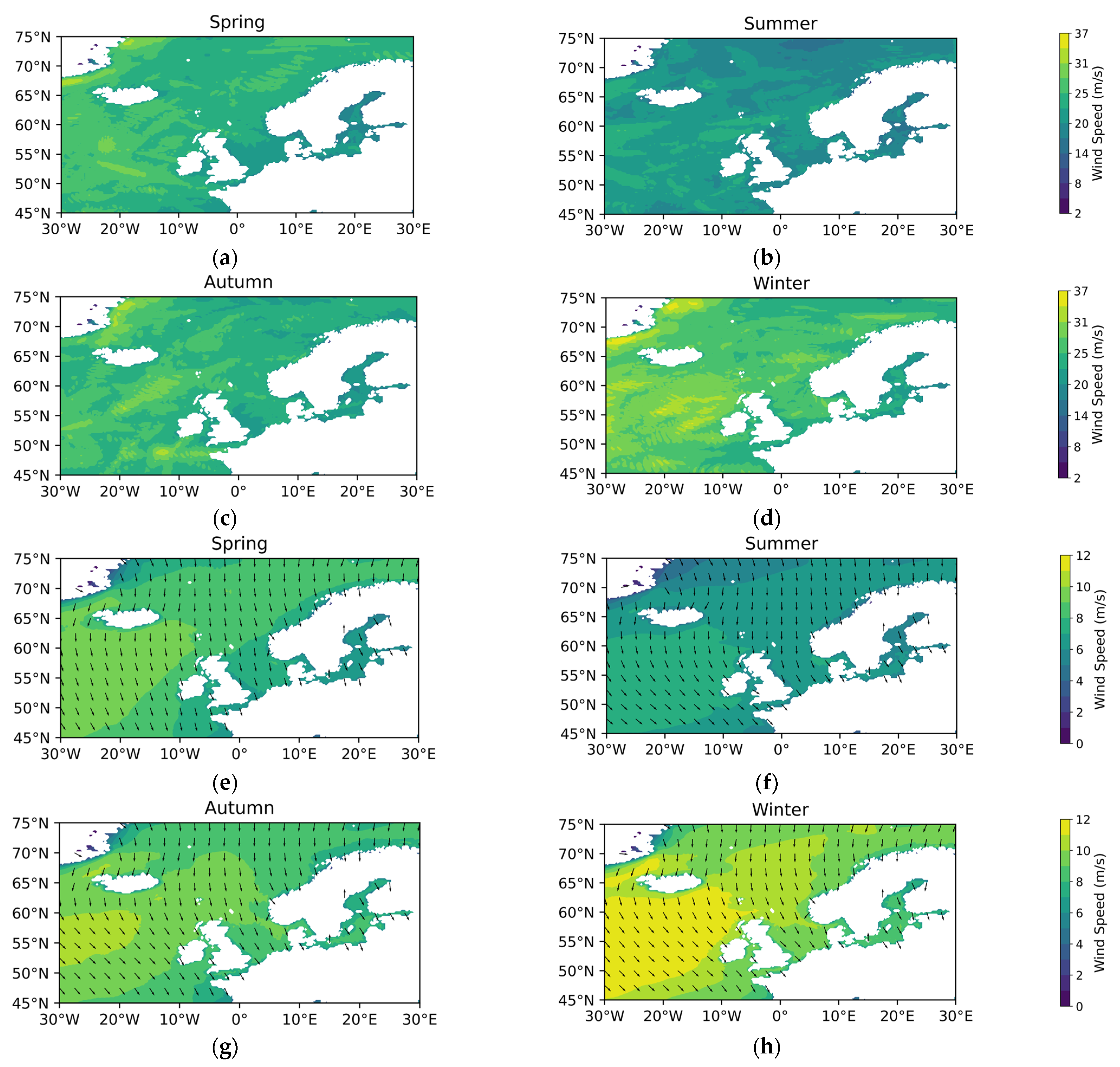
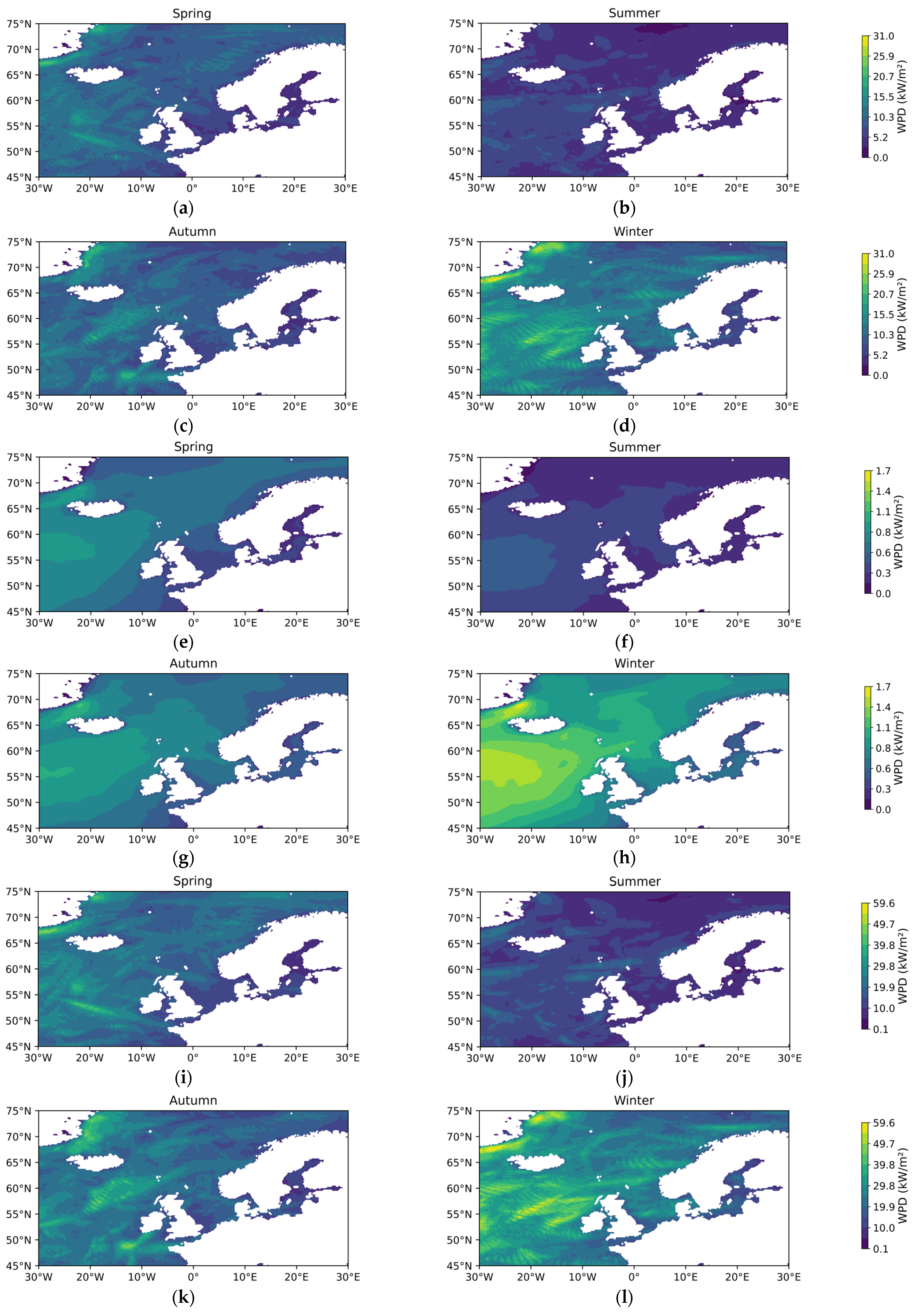
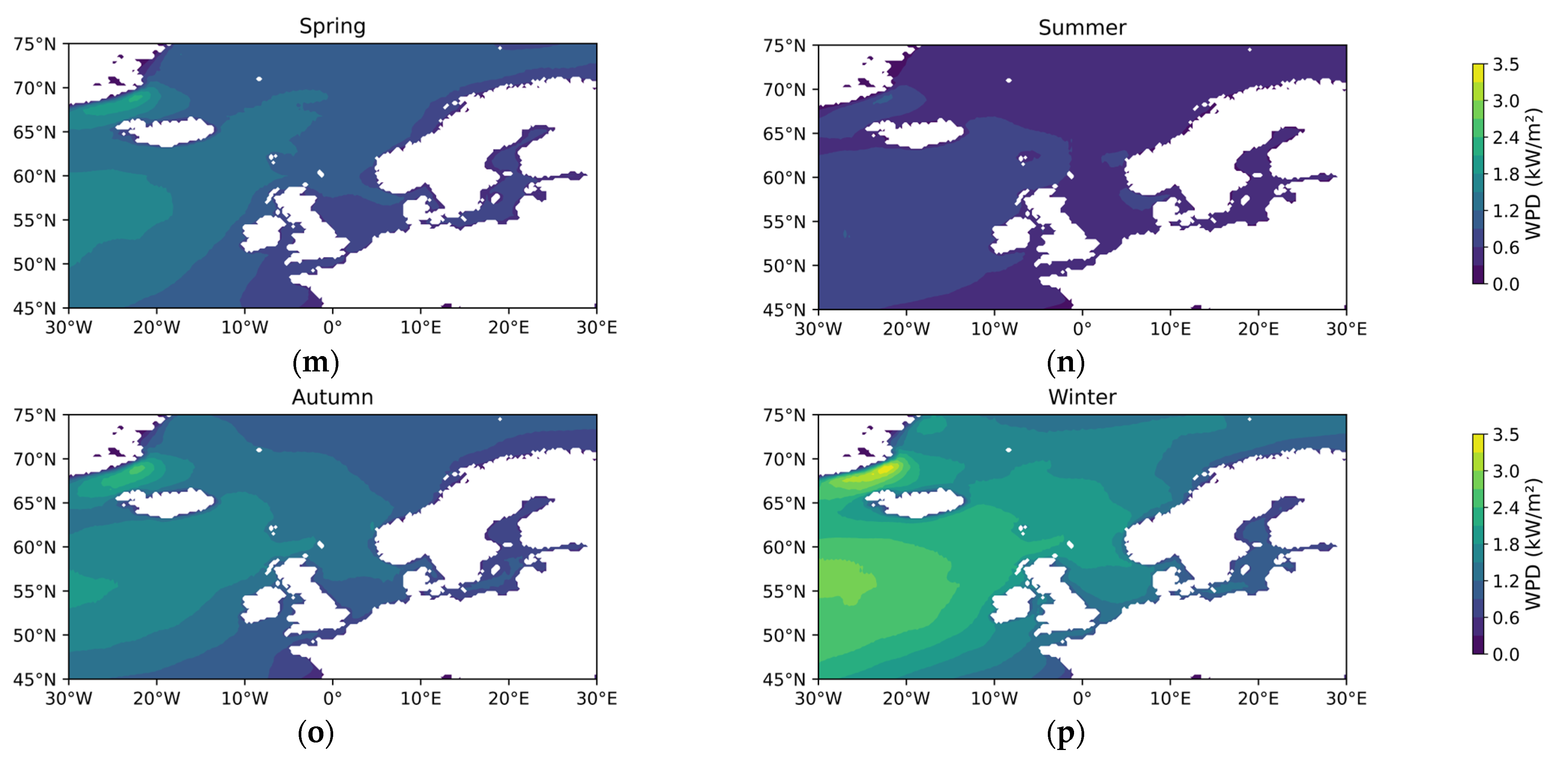
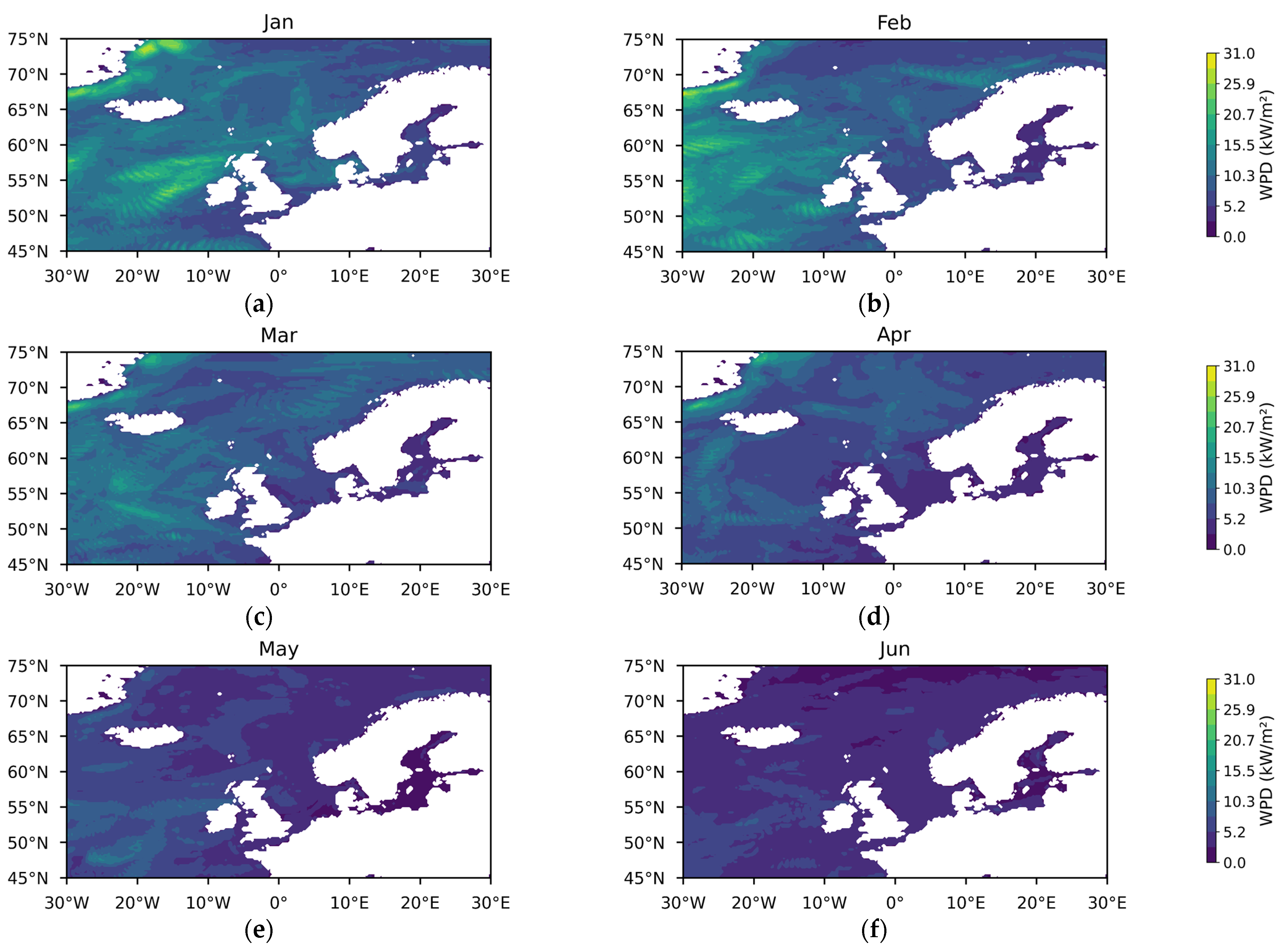
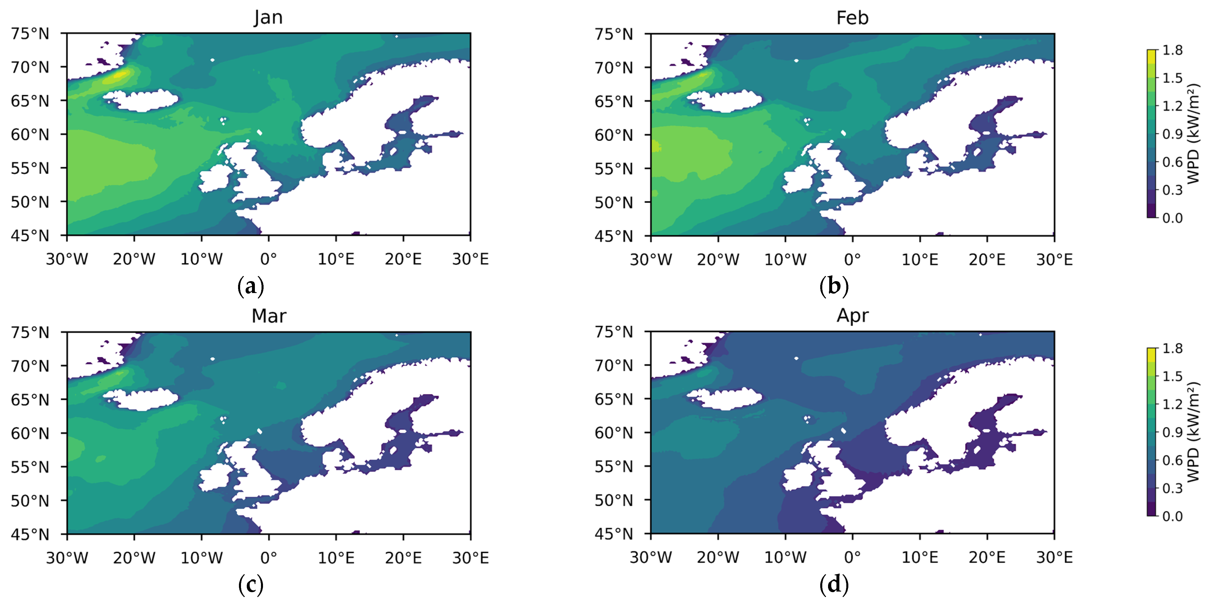
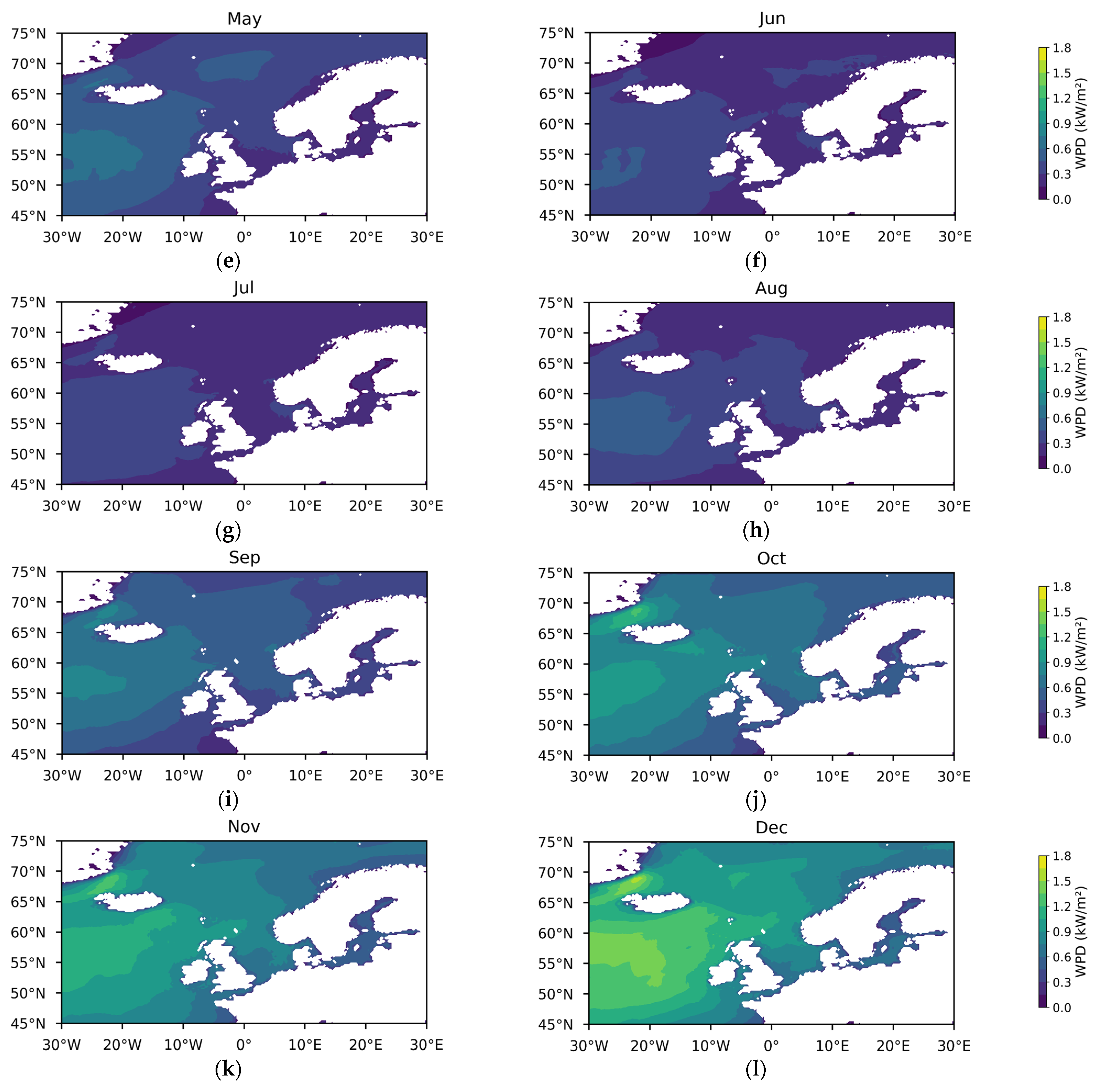
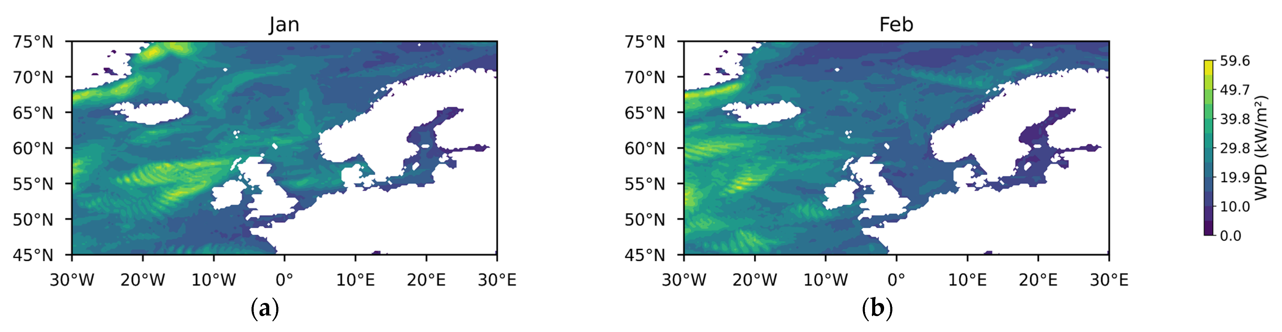
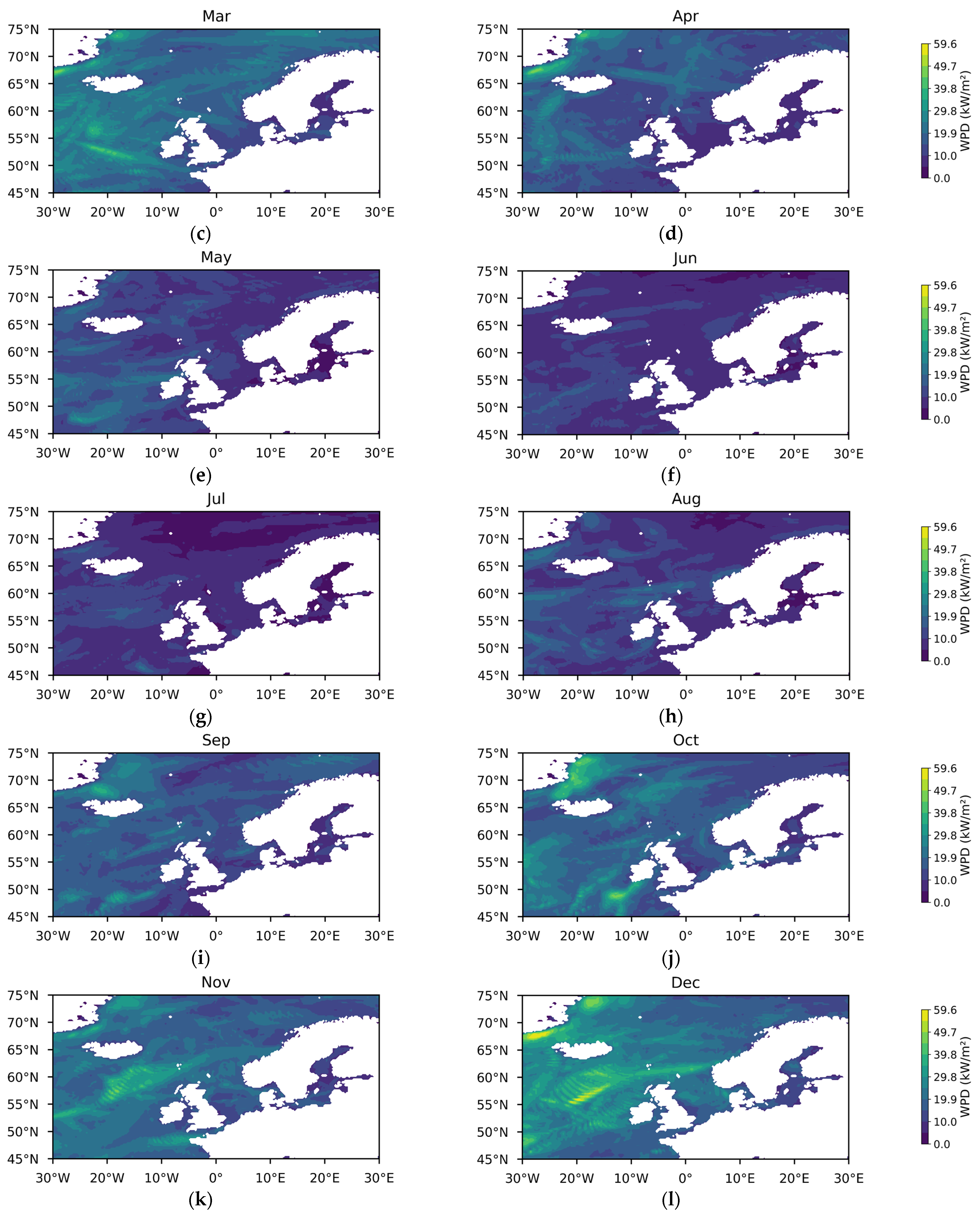
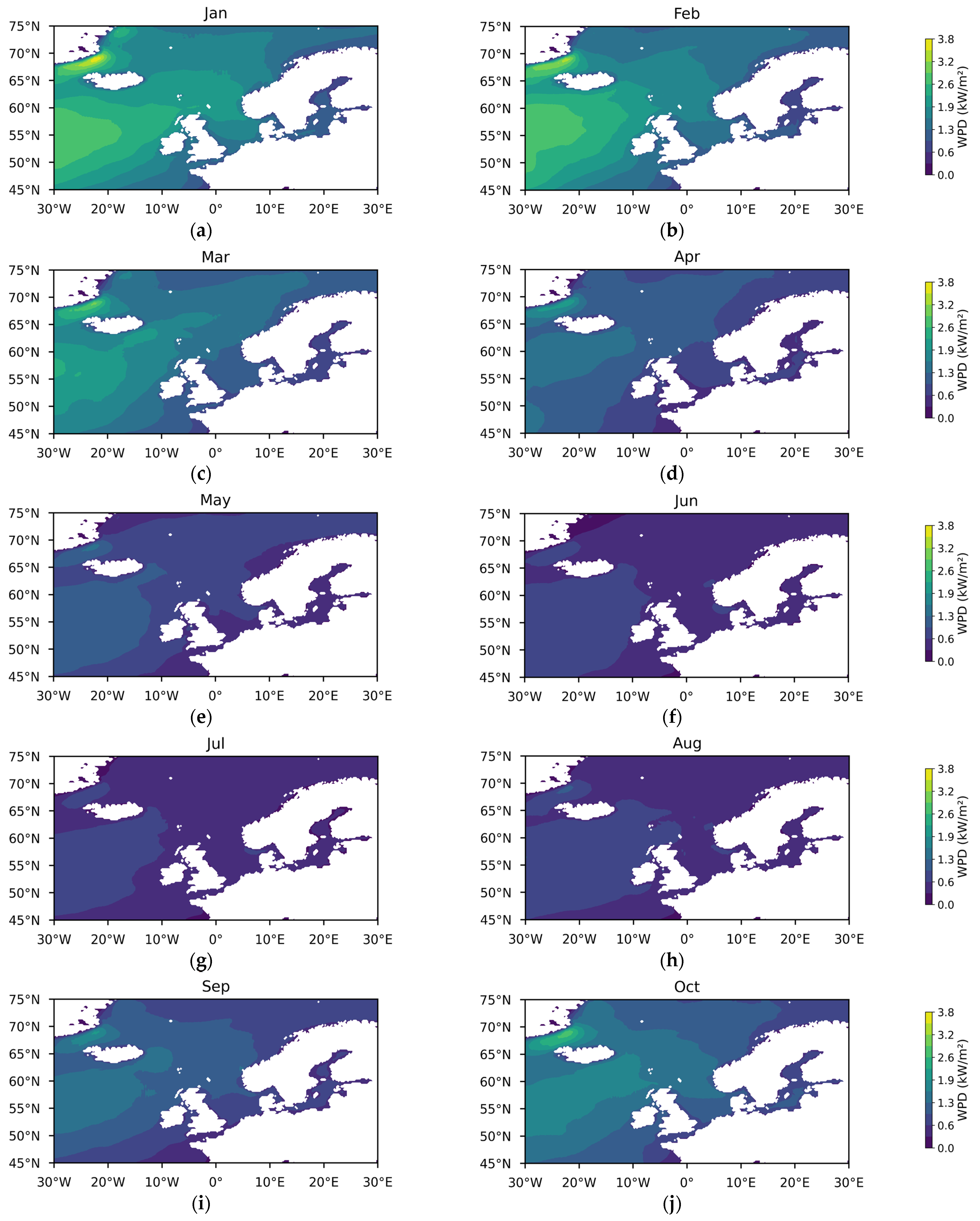
3.1.1. Theoretical Potential of Wind Energy

Wind speed, wind direction, WPD, and EWSO are crucial indicators in the evaluation of wind energy resources. These factors influence turbine efficiency, spatial layout, and the long-term economic viability of wind farms. Wind energy distribution globally is driven by complex interactions of meteorological and geographical conditions, highlighting the need for thorough analysis to maximize energy capture.

The multiyear analyses (Figure A1 and Figure A7) indicate that average wind speeds at 100 m above sea level (ASL) in the southeastern coastal areas of China and the Taiwan Strait range from 10 to 12 m/s, together with 7 to 9 m/s at 10 m ASL. These regions exhibit richer wind energy resources at higher altitudes, making them particularly suitable for the development of large-scale wind farms. In addition, the southeastward and eastward winds during the summer monsoon dominate the wind patterns, promoting a more consistent wind energy distribution. Additionally, the EWSO analysis (Figure A13) reveals that these regions have high wind energy utilization rates, especially in the seas east of Jiangsu–Zhejiang and Hainan, where EWSO typically exceeds 0.95. This suggests that wind speeds generally remain within the optimal operating range for turbines.

However, seasonal variations (Figure A2, Figure A3, Figure A4, Figure A5, Figure A6, Figure A8, Figure A9, Figure A10, Figure A11, Figure A12, Figure A14, Figure A15 and Figure A16) show significant fluctuations. During summer, despite a peak in WPD, EWSO drops to around 0.9 in the southern Yellow Sea and East China Sea, as high wind speeds occasionally exceed turbine cut-out speeds, leading to shutdowns. This phenomenon limits effective wind energy utilization despite the theoretical potential indicated by WPD.

In contrast, wind energy resources in the European sea areas are more stable. The North Sea, Baltic Sea, and Atlantic coast exhibit relatively uniform wind speed distribution year-round, with wind speeds typically ranging from 7 to 12 m/s (Figure A18, Figure A19, Figure A20, Figure A21, Figure A22 and Figure A23). Although WPD (Figure A24, Figure A25, Figure A26, Figure A27, Figure A28 and Figure A29) in summer generally does not exceed 10 kW/m², EWSO (Figure A30, Figure A31, Figure A32 and Figure A33) remains close to 1, indicating that wind speeds stay within the effective operating range of turbines for most of the time, ensuring efficient wind energy utilization. For example, in the northern UK seas during summer, despite high average wind speeds, WPD is not necessarily high due to the low volatility of the wind speed. However, as wind speeds remain within the optimal operating range of turbines, effective wind energy utilization hours are higher. This nonlinear relationship (WPD ∝ V³) suggests that small changes in the wind speed could affect WPD significantly, and the stability of wind speeds is the key factor in determining overall power generation efficiency.

In summary, while wind speed and WPD are important for evaluating wind resources, a comprehensive analysis of EWSO and wind speed variability is essential for a more accurate assessment of wind energy potential. This research highlights the importance of considering temporal and spatial variations in wind speeds and energy utilization to better understand wind resource characteristics.

3.1.2. Temporal and Spatial Variability in Wind Energy Stability

Section 3.1.1 discusses spatial distribution differences. As shown in Figure 1, the annual variations in WPD exhibit significant spatial and temporal fluctuations. This section focuses on the impact of wind resource variability on model selection, aiming to better understand wind speed fluctuations and optimize wind energy assessments.

The coefficient of variation (CV) of daily wind speeds is a key indicator for assessing wind energy stability (Figure A17a,b). A clear north–south discrepancy is evident in China’s offshore regions. The northern coastal areas of Fujian show CV values greater than 1.3, indicating higher wind speed variability. In contrast, the Taiwan Strait exhibits lower CV values, reflecting more stable wind speeds with smaller daily fluctuations, contributing to greater resource stability.

Seasonal and monthly variations in wind energy resources are also significant. The seasonal variability index (SVI) and monthly variability index (MVI) (Figure A17c–f) highlight the influence of the South China Sea monsoon, which causes greater fluctuations in the southern regions, particularly during the southwest monsoon period [57]. These fluctuations reduce wind energy stability compared to northern areas.

In the European seas, the CV values are generally higher than 1.3 (Figure A34a,b). However, wind speed variability is more uniformly distributed across the region, with no significant spatial differences. The SVI typically exceeds 1.0, and the MVI is usually above 1.2, indicating notable seasonal and monthly variability (Figure A34c–f). Despite this, wind resources show consistent temporal fluctuations across Europe, likely due to the stabilizing effect of the Atlantic Ocean. The large Atlantic Ocean and prevailing westerly winds lead to more predictable wind patterns, ensuring relatively stable wind resources throughout the year.

In contrast, China’s offshore wind resources are heavily influenced by monsoons and typhoons, creating remarkable north–south differences. The seasonal monsoons, especially the southwest monsoon, cause greater variability in the south, while typhoons bring abrupt fluctuations, further increasing the temporal and spatial variability in wind resources.

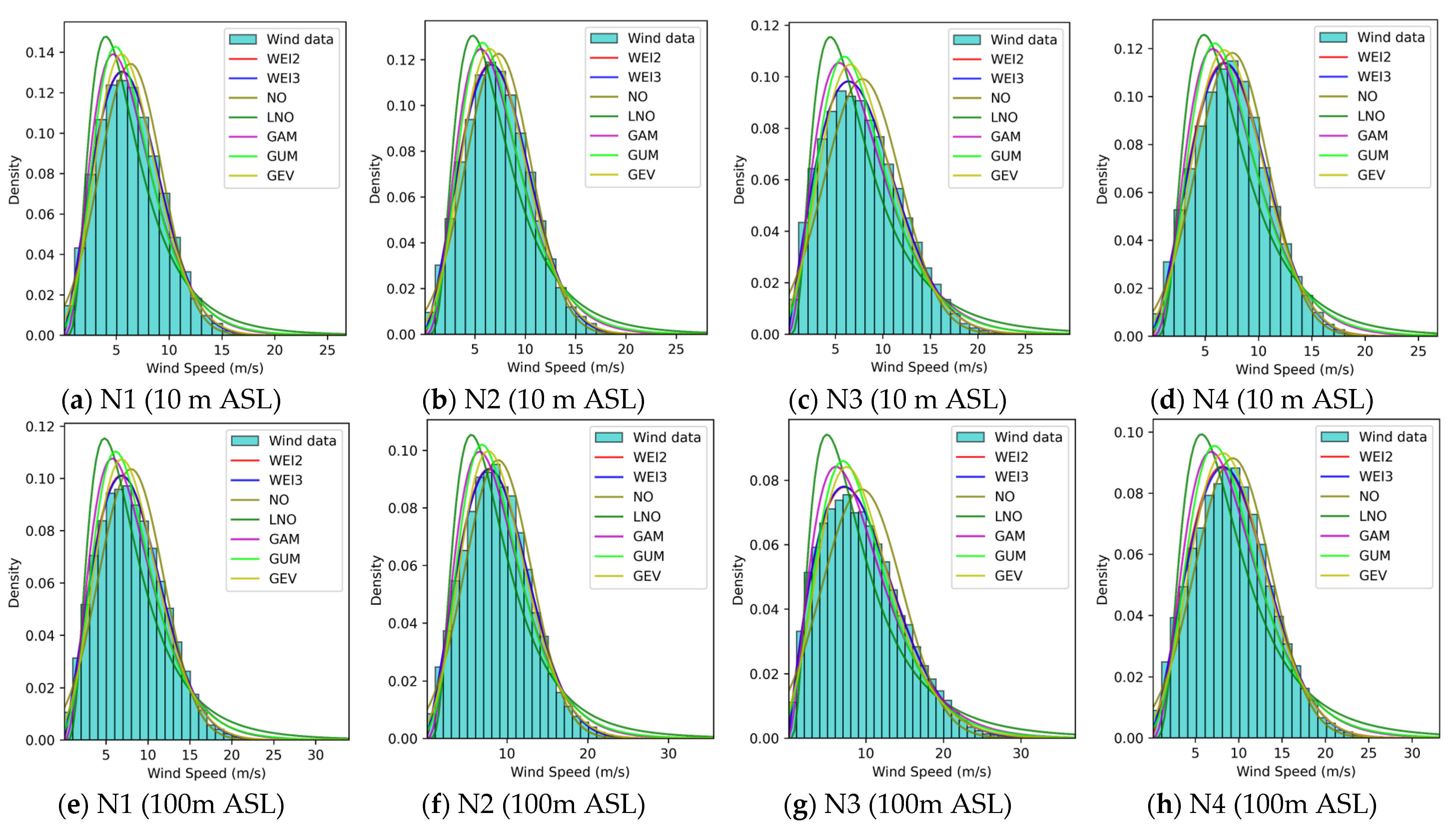
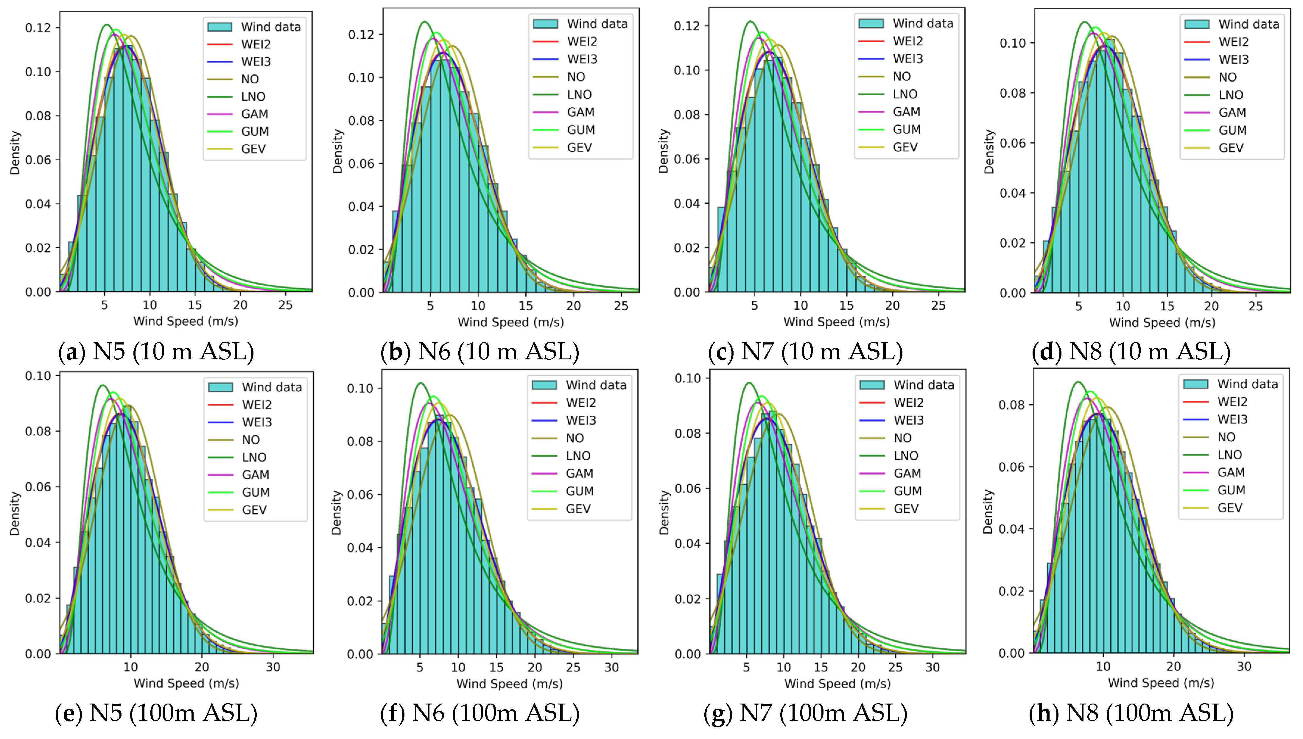
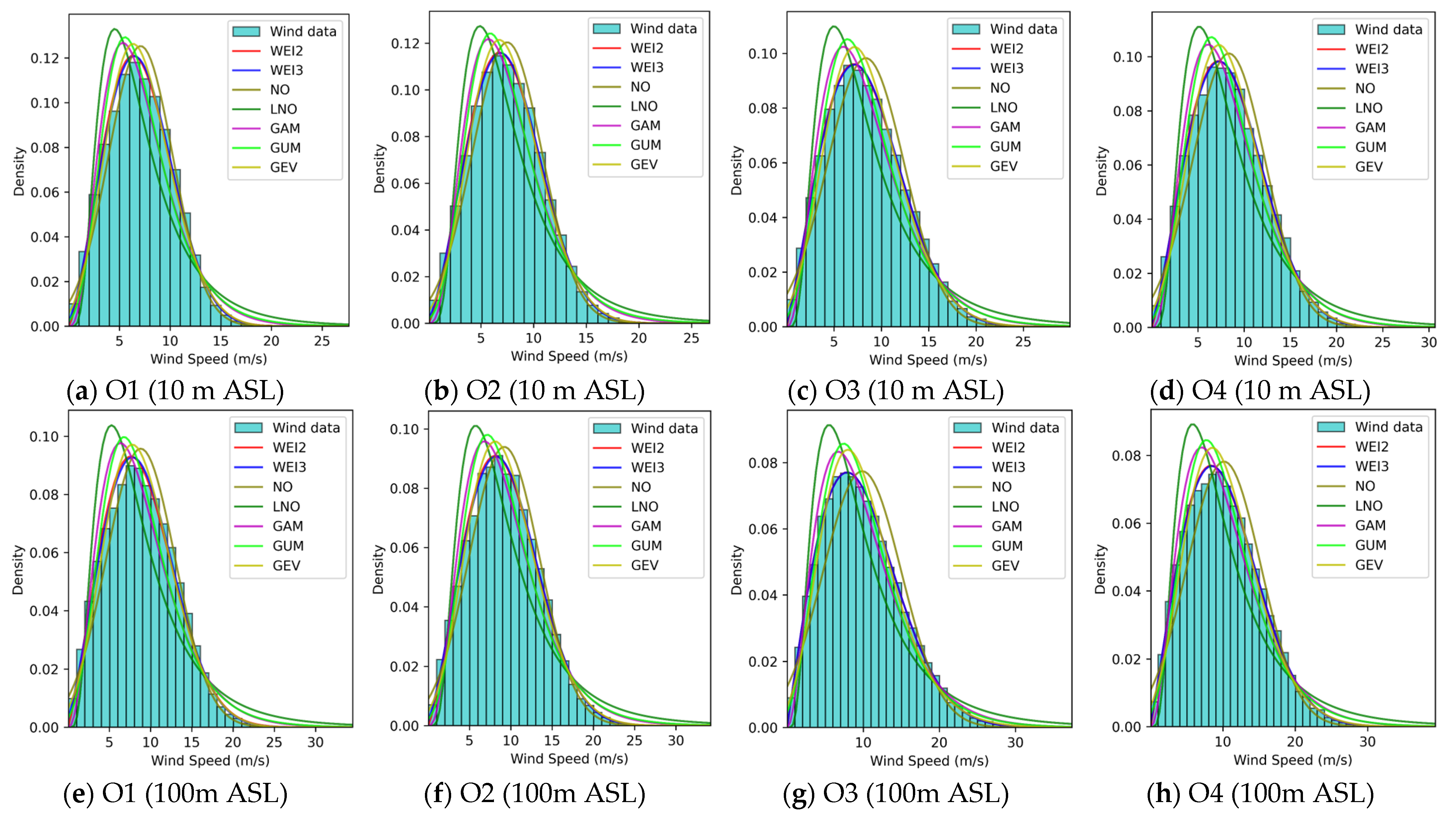
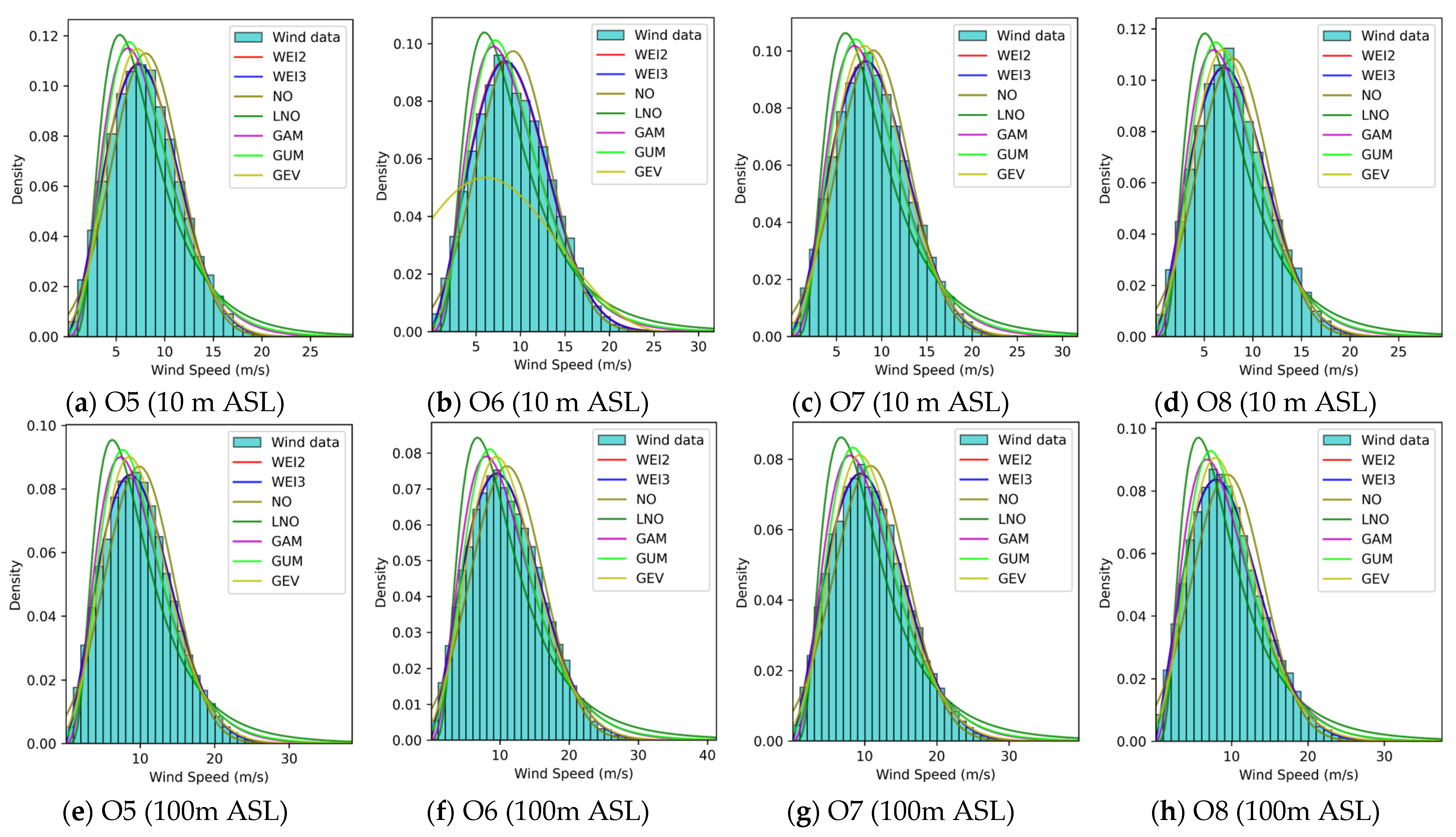
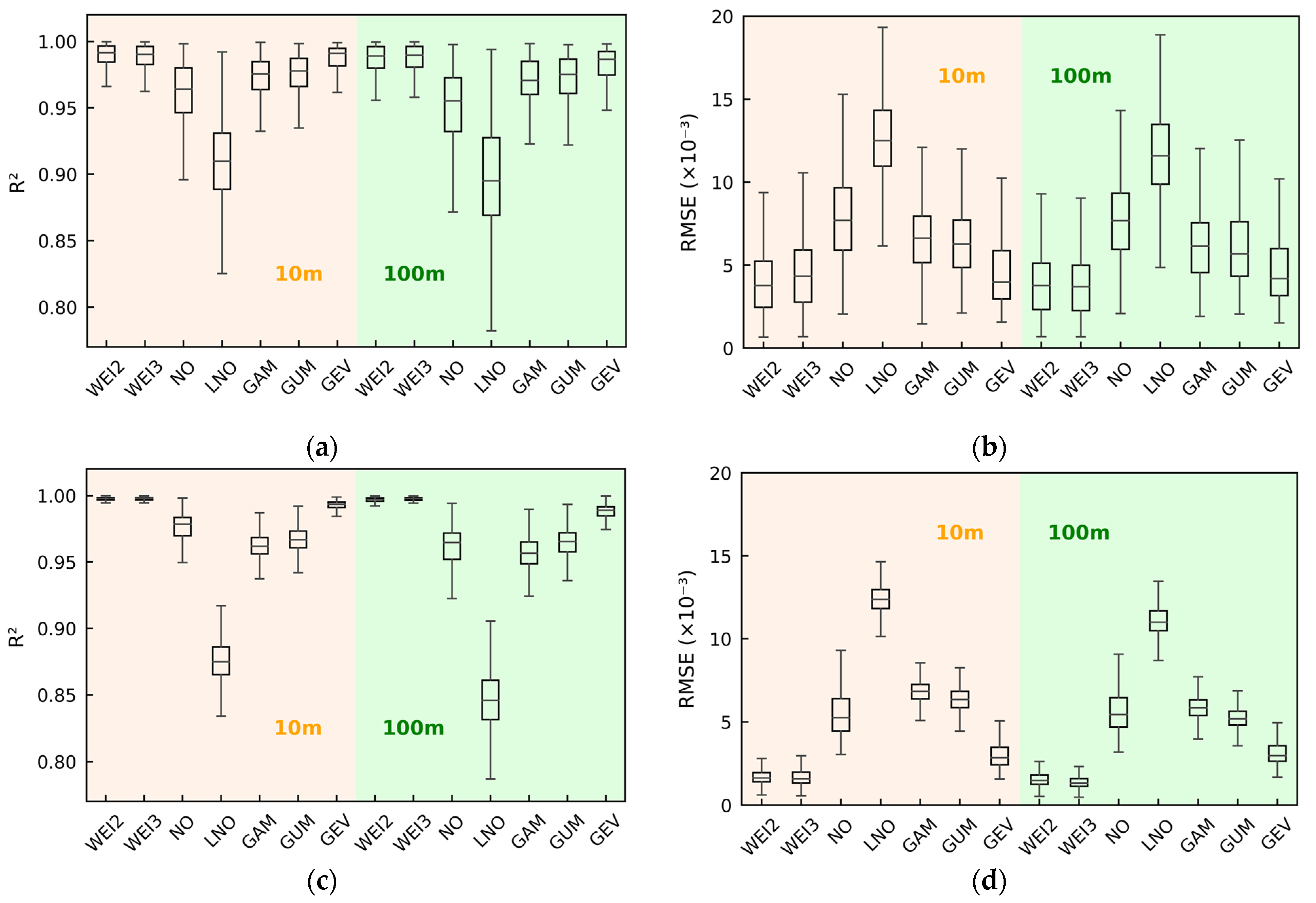
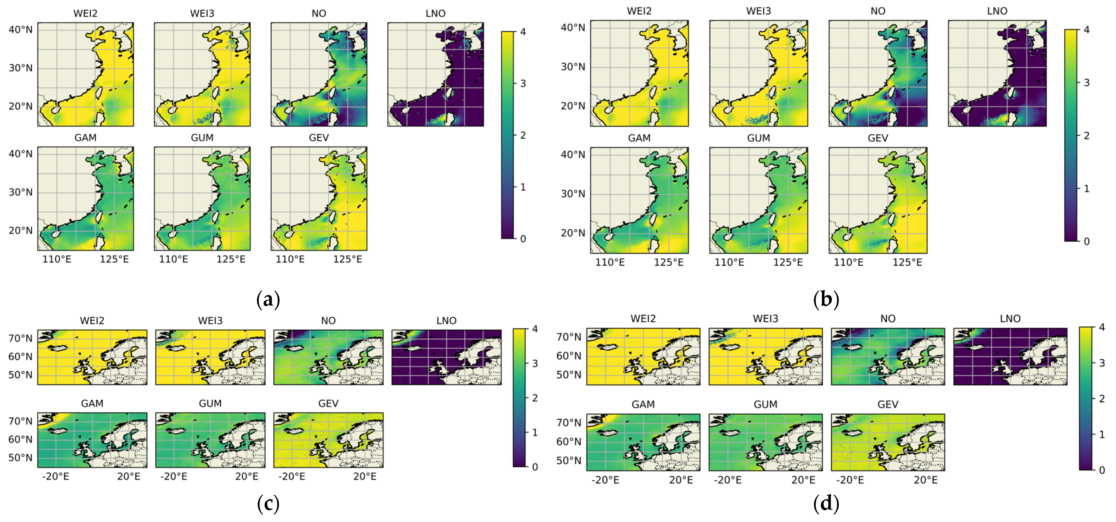
3.2. Comprehensive Performances of WSPD Models

In this section, we evaluate the performances of different wind speed probability distribution (WSPD) models, as listed in Table 1, at two different heights (10 m ASL and 100 m ASL) over a 20-year period. To ensure computational efficiency, data from four representative times each day (00:00, 06:00, 12:00, and 18:00 UTC) were used, capturing the key characteristics of wind speed variation.

The results, summarized in boxplots (Figure 2), show that the WEI-class models (WEI2 and WEI3) consistently perform well, with higher R² values and lower RMSE. At 10 m ASL, WEI2 slightly outperforms WEI3, although this difference is less significant in the European seas. However, at 100 m ASL, WEI3 outperforms WEI2, demonstrating its better ability to handle wind speed distributions at higher altitudes. The GEV model also performs competitively, especially in regions with high variability and extreme wind events. In contrast, the NO and LNO models show higher RMSE and lower R² values, indicating poor fit for the wind speed distributions in these regions. The WEI-class models better capture the wind speed patterns, reflecting the moderate to high wind speeds with occasional extremes.

The selected grid cells for model fitting, shown in

Table 2. Coordinates of the points in Figure 3.

	Index	Coordinates (CHN)	Coordinates (EU)
nearshore points	N1	(38.75° N, 118.00° E)	(63.00° N, 19.00° E)
	N2	(37.50° N, 122.75° E)	(55.00° N, 19.00° E)
	N3	(35.00° N, 119.50° E)	(60.00° N, 4.00° E)
	N4	(31.00° N, 122.25° E)	(55.00° N, 0.50° W)
	N5	(24.25° N, 118.50° E)	(54.00° N, 6.00° E)
	N6	(23.50° N, 121.75° E)	(50.50° N, 1.00° E)
	N7	(20.25° N, 110.00° E)	(53.00° N, 5.50° W)
	N8	(21.25° N, 109.00° E)	(53.00° N, 11.00° W)
offshore points	O1	(38.50° N, 120.00° E)	(61.00° N, 19.50° E)
	O2	(38.50° N, 123.00° E)	(56.00° N, 19.00° E)
	O3	(35.50° N, 123.75° E)	(65.00° N, 5.00° E)
	O4	(31.50° N, 125.00° E)	(58.50° N, 1.00° E)
	O5	(27.00° N, 124.00° E)	(55.00° N, 4.00° E)
	O6	(21.00° N, 119.00° E)	(60.00° N, 8.00° W)
	O7	(19.00° N, 113.00° E)	(52.00° N, 13.00° W)
	O8	(18.00° N, 117.00° E)	(47.50° N, 8.00° W)

and Figure 3, cover a range of coastal and offshore locations across China and Europe. These locations were chosen to represent different wind regimes. Figure A35, Figure A36, Figure A37, Figure A38, Figure A39, Figure A40, Figure A41 and Figure A42 display the wind speed distributions at these selected points, highlighting the variability and distinct distribution types in the regions.

• Wind speed patterns in China seas.

The wind speed distributions in coastal areas of China exhibit significant variability at 10 m ASL (

Table 3. Statistical properties of the wind speed of selected points in Chinese sea areas.

	10 m ASL				100 m ASL
	Mean	Variance	Skewness	Kurtosis	Mean	Variance	Skewness	Kurtosis
N1	5.3491	6.4417	0.6847	0.5447	6.5539	10.6193	0.6024	0.1909
N2	6.1297	9.3071	0.5427	−0.0209	7.4772	14.0968	0.4441	−0.2053
N3	4.7815	5.2563	0.6847	0.5574	5.9377	8.5579	0.5544	0.1820
N4	6.3413	7.5491	0.4591	0.3367	7.7209	12.4279	0.5177	0.4294
N5	7.9714	15.3298	0.1333	−0.8964	9.5660	20.8942	0.0883	−0.7274
N6	5.9744	14.8770	0.6734	−0.2009	6.7701	21.0287	0.8165	0.3160
N7	4.2126	3.5845	0.5293	1.3325	5.8562	6.5856	0.4555	1.6242
N8	5.3760	7.7344	0.5790	0.2541	6.3135	10.6380	0.6457	0.6886
O1	5.9781	8.3171	0.5838	0.1921	7.3904	13.7411	0.5252	−0.0700
O2	6.1286	8.9178	0.4454	−0.2449	7.4041	13.7975	0.4146	−0.2954
O3	6.1595	10.1012	0.5701	−0.0145	7.3104	15.1018	0.5735	0.0684
O4	6.6838	9.6816	0.5265	0.3435	8.0290	14.6057	0.5748	0.7700
O5	7.5259	10.1073	0.5856	1.1038	8.6803	14.6588	0.8267	2.6348
O6	7.5523	10.9725	0.0840	−0.2759	8.5766	15.4635	0.2303	0.2020
O7	7.1267	9.9827	0.3753	−0.0736	8.1351	14.1181	0.4574	0.3078
O8	7.2561	15.1524	0.3185	−0.6642	8.3505	22.4485	0.4089	−0.5066

). Specifically, at N1 (Bohai Bay), the mean wind speed is 5.35 m/s with a skewness of 0.68, indicating occasional strong winds. At N2 (Shandong Peninsula), the mean wind speed is 6.13 m/s with a skewness of 0.54, indicating a more stable wind profile. In contrast, at N5 (Taiwan Strait), the mean wind speed is 7.97 m/s with a variance of 15.33, reflecting higher wind energy potential coupled with frequent extreme wind events. At 100 m ASL, the mean wind speeds increase significantly, with 6.55 m/s at N1, 7.48 m/s at N2, and 9.57 m/s at N5, but the variability remains notable, particularly in the N5 and N6 regions. Offshore regions exhibit more stable wind conditions. For example, at O1 (Bohai Sea), the mean wind speed at 10 m ASL is 5.98 m/s with a skewness of 0.58. It rises to 7.39 m/s at 100 m ASL with a skewness of 0.53. At O5 (South East China Sea), the mean wind speed at 10 m ASL is 7.53 m/s with a skewness of 0.59. It increases to 8.68 m/s at 100 m ASL with a skewness of 0.83, indicating a more uniform wind profile. However, at O8 (South China Sea), the wind speed at 100 m ASL shows significant variability, with a variance of 22.45. This phenomenon indicates that considerable fluctuations could emerge at higher altitudes.

The histogram analysis reveals that the wind speed distributions at N5, O6, and O8 exhibit distinct multimodal patterns, indicating complex wind speed characteristics that cannot be adequately captured by common unimodal distribution models (such as WEI-class or GAM). Multimodal distributions typically suggest that wind speed variations in these areas may be influenced by multiple factors, such as seasonal changes, alternating climate systems, or topographical effects [27]. Therefore, in these regions, the evaluation of models based on single-peak distributions may not be appropriate, and a different approach is needed to reflect the complex wind speed variability.

In contrast, at N6 (eastern Taiwan), the wind speed distribution shows a significant right-skewed pattern, particularly at 10 m ASL. The mean wind speed is relatively low, resulting in a more pronounced right skew. This wind speed distribution is distinct from other locations. For such distributions, the Gamma distribution model provides a better fit compared to the WEI-class models, as the GAM model is more suitable for low wind speeds with right-skewed characteristics. Overall, coastal regions in China are influenced by monsoons and typhoons, leading to significant wind speed fluctuations, especially at lower altitudes. Offshore areas, particularly at higher altitudes, exhibit more stable wind conditions, making them more suitable for large-scale wind farm development.

2.

Wind speed patterns in European seas.

The statistical properties of wind speed at 10 m and 100 m ASL across selected EU points show consistently slightly right-skewed distributions, in contrast to the more variable, multimodal distributions in China’s coastal regions (

Table 4. Statistical properties of the wind speed of selected points in European sea areas.

	10 m ASL				100 m ASL
	Mean	Variance	Skewness	Kurtosis	Mean	Variance	Skewness	Kurtosis
N1	6.3564	8.8171	0.4301	−0.1323	7.9894	14.8194	0.4246	−0.1486
N2	7.3191	10.5888	0.3808	−0.0385	8.8885	17.0481	0.4691	0.1899
N3	7.8580	16.2005	0.4742	−0.2504	9.4819	26.7340	0.5759	−0.0844
N4	7.5491	11.3857	0.3259	−0.2143	9.3209	19.0244	0.3669	−0.1564
N5	7.9163	11.7771	0.3091	−0.1802	9.6757	19.9670	0.4314	−0.0037
N6	7.2980	12.0184	0.3809	−0.2507	8.8808	19.7093	0.5096	0.0307
N7	7.5376	12.8315	0.3741	−0.2251	9.2352	20.9977	0.4971	0.05357
N8	8.7466	15.0919	0.3507	−0.1499	10.5704	25.3312	0.4538	−0.0624
O1	7.0874	10.1322	0.3007	−0.2524	8.8142	17.3472	0.3258	−0.2795
O2	7.4992	10.9823	0.3215	−0.1980	9.2120	18.0297	0.3815	−0.0617
O3	8.3569	16.4719	0.4483	−0.1678	9.8636	26.5421	0.5962	0.07529
O4	8.3489	15.5360	0.4102	−0.1952	10.1472	26.0047	0.4874	−0.0892
O5	8.0455	12.4473	0.3551	−0.1971	9.8697	20.9753	0.4486	−0.0284
O6	9.1660	16.7673	0.3310	−0.2690	10.9947	27.2762	0.4267	−0.1320
O7	9.0514	15.8313	0.3587	−0.1687	10.8327	26.0596	0.4573	−0.0669
O8	7.9743	13.5199	0.4336	−0.1075	9.4651	21.8541	0.5491	0.0691

). At 10 m ASL, the mean wind speeds range from 6.36 m/s at N1 (Baltic Sea) to 8.75 m/s at N8 (Western Ireland). As the altitude increases, the variance also rises, reflecting more pronounced wind speed fluctuations. At 100 m ASL, the mean wind speed increases, reaching 9.68 m/s at N5 (near the Netherlands) and 10.99 m/s at O6 (offshore UK). Offshore sites exhibit relatively stable wind conditions despite considerable variance at some locations (e.g., variance of 27.28 at O6). Despite this, the distributions remain right-skewed.

Given these characteristics, the WEI-class models (such as WEI2 and WEI3) provide the best fit for the data. These models are particularly well-suited to the stable distributions in the European sea areas.

3.

Summary.

The comparison of wind speed distributions between the Chinese and European coastal and offshore regions reveals some differences. The Chinese coastal areas show higher variability and multimodal distributions, particularly in the Taiwan Strait and South China Sea. In contrast, the European regions exhibit more stable, slightly right-skewed distributions, which are well captured by the WEI-class models. Offshore areas in Europe, especially at higher altitudes, offer more stable and predictable wind conditions, where large-scale wind energy development is feasible.

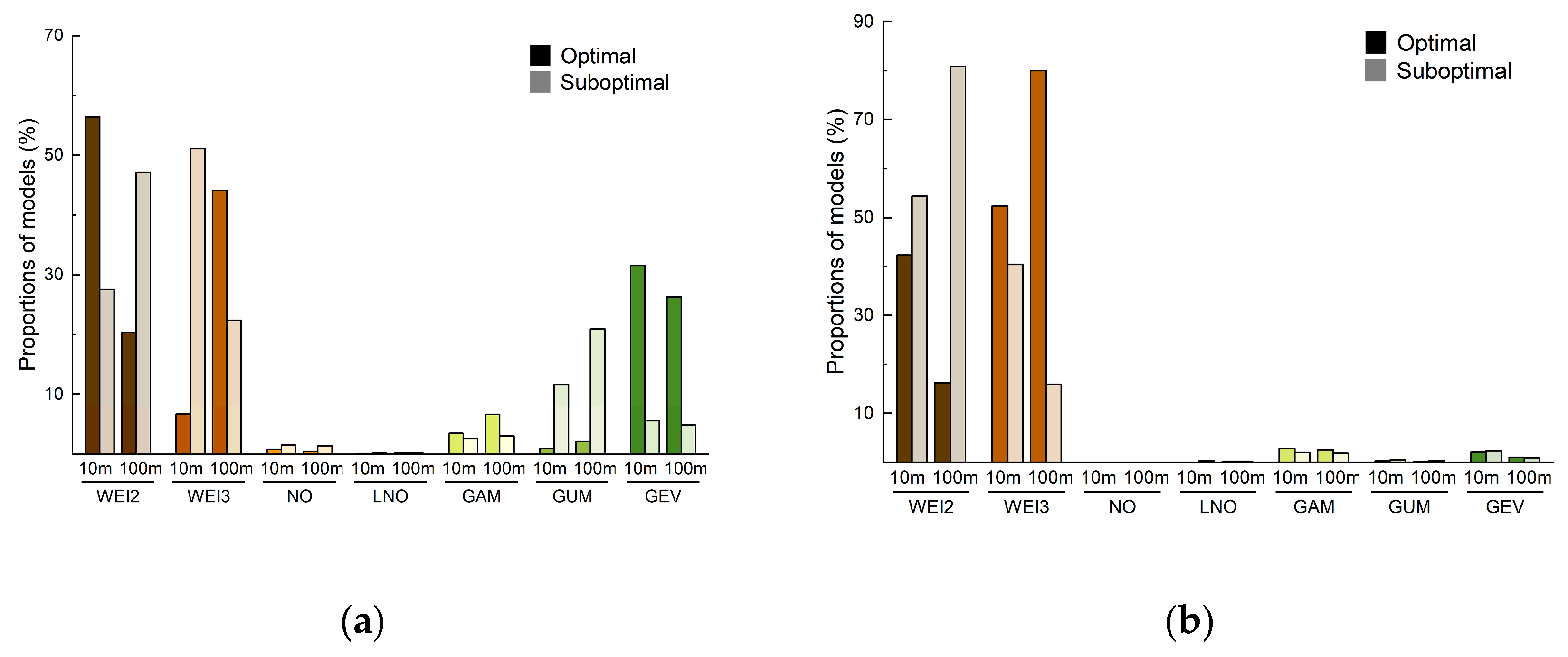
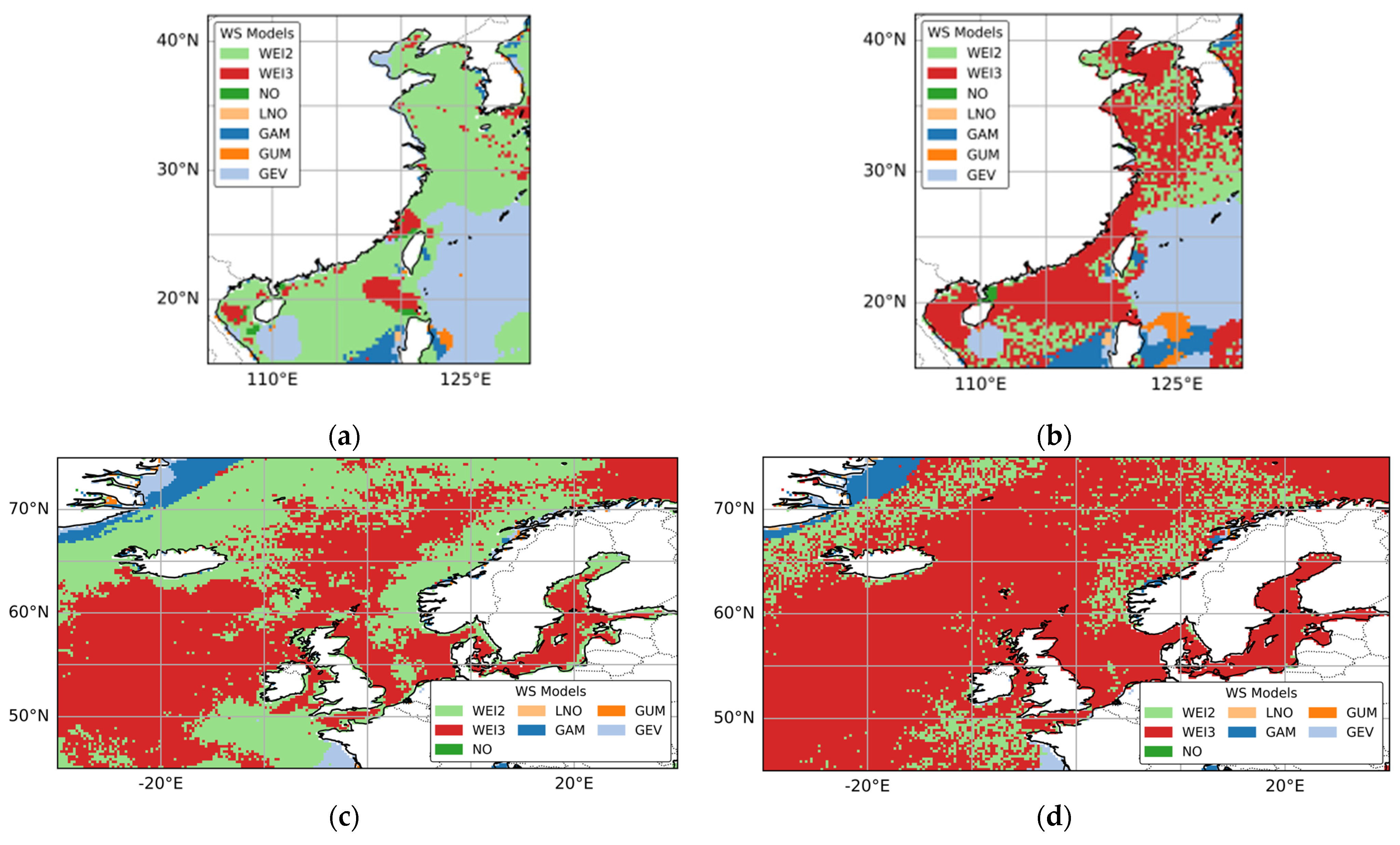
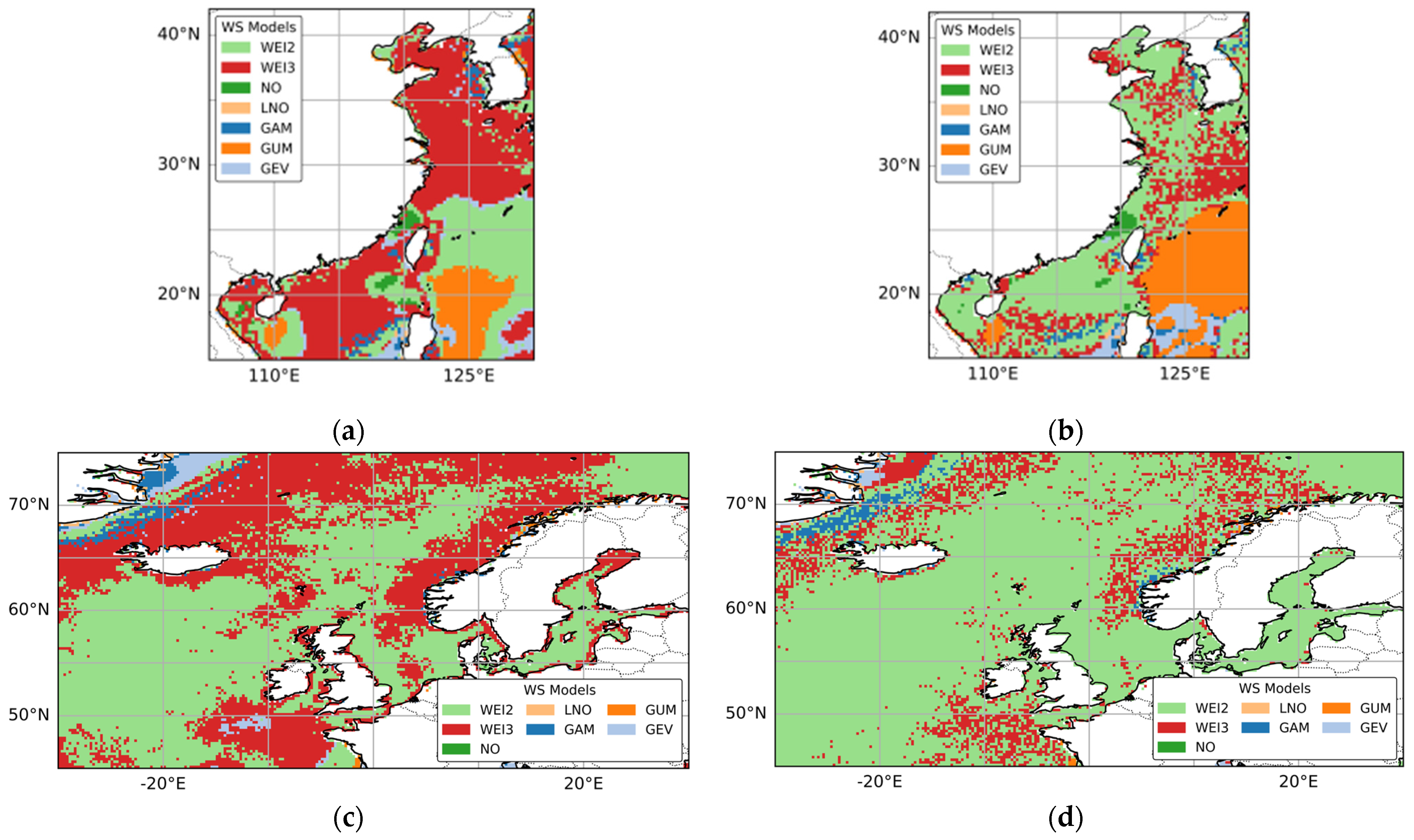
3.3. Distributions of Optimal and Suboptimal WSPD Models

In this section, we assess the performances of the selected wind speed probability distribution (WSPD) models by calculating their normalized scores based on R², RMSE, AIC, and BIC values. Each metric was equally weighted, yielding a total score ranging from 0 to 4, where higher scores indicate better model performances. The distribution of these scores at both 10 m ASL and 100 m ASL across the Chinese and European offshore regions is shown in Figure 4.

The results reveal significant regional differences. In both regions, the WEI-class models consistently achieve the highest scores. In China, the distribution of model scores is less uniform compared to Europe. Although WEI2 and WEI3 have the best performances, the broad spread of scores suggests that the wind speed characteristics with greater spatial and temporal variability are more challenging to model. This is likely due to China’s complex coastal topography and the high variability in wind speeds. In contrast, the distribution in Europe is more uniform, reflecting stable wind speed patterns.

To further assess the models’ performances, we examined the frequency of the most optimal and suboptimal models across different grid points. Figure 5 illustrates the frequency distribution of the optimal and suboptimal models at both 10 m ASL and 100 m ASL. In China, WEI2, WEI3, and GEV are the most frequent optimal models. The spatial distributions of the optimal and suboptimal models, shown in Figure 6 and Figure 7, reveal that the GEV model is mainly found in the East China Sea, the adjacent western Pacific, and the southern sea region of Hainan Island. In these regions, GUM is always the suboptimal model, suggesting that GEV and GUM share similar characteristics. This is supported by the behavior of the O5 point (Section 3.2) in the East China Sea, where GEV fits the wind speed distribution, which is characterized by high kurtosis and relatively low mean wind speeds. This distribution indicates local low wind speeds with occasional extreme events, which is effectively captured by the GEV model, known for modeling extreme values or tail events. The GUM model, selected as a suboptimal model, shares similarities with the GEV model in capturing high peak and moderate tail behavior. However, as a two-parameter distribution, GUM is less flexible compared with the GEV model. Since the GEV model is a three-parameter distribution, it is more suitable in terms of extreme wind events and tail behavior modeling, making GEV the optimal choice in these cases. Similarly, WEI3 often outperforms WEI2 for similar reasons, as its additional parameter provides greater flexibility in capturing complex wind speed distributions.

In Europe, the WEI-class models again dominate the optimal and suboptimal model selections. The consistent performance across regions further highlights the stability of wind conditions in Europe, where WEI2 and WEI3 emerge as the most suitable models for wind speed distributions at both altitudes. This suggests that wind speed distributions in the European offshore areas are more uniform, making them easier to model with simpler, well-established distributions like WEI-class models. The stability of wind conditions in Europe allows for a more simple application of these models, while in China, the complex variability in wind speeds requires a more flexible modeling approach.

3.4. Guidelines for Selecting the Optimal WSPD Model

Wind speed characteristics, including mean wind speed, variance, skewness, and kurtosis, vary significantly across different regions, influencing the selection of the optimal wind speed probability distribution (WSPD) model. In the Chinese seas (Figure 8), wind speed distributions are more variable, with higher skewness and kurtosis values, particularly in coastal areas like the Taiwan Strait and the South China Sea, where extreme wind events are more frequent. In contrast, the European seas (Figure 9) are characterized by higher variance, indicating more fluctuations in wind speed, but with lower skewness and kurtosis compared to China. These regional differences underline the importance of considering specific wind speed characteristics when choosing the most suitable WSPD model.

In the analysis of wind speed characteristics at 10 m ASL and 100 m ASL in the Chinese seas (Figure 10), most models, particularly those based on Weibull distributions, exhibit a positive correlation between the mean wind speed and variance. This suggests that as the mean wind speed increases, the variance in the wind speed also increases. Concurrently, as the mean wind speed rises, both skewness and kurtosis tend to decrease. This implies that at higher wind speeds, the distributions become more symmetric with lighter tails. This indicates that the frequency of extreme high wind speed events is lower. On the contrary, the GEV model’s concentration in regions with high skewness and kurtosis suggests that this model may be more effective in capturing the positively skewed characteristics. Therefore, it might have good performances in regions where extreme wind speed events are more frequent.

For the European seas (Figure 10), the Weibull-based models dominate. Different from the Chinese seas, the GAM distribution model is more effective in regions with higher variance, kurtosis, and skewness, such as the eastern Greenland seas. This suggests that the wind speed distribution in these regions is positively skewed, probably influenced by the unique climatic conditions (e.g., polar and marine climates [47,67]), topographic features (e.g., Greenland’s mountains [68]), and ocean dynamics (e.g., ocean currents, tides, and vortices [69]), which directly influence wind loads [70,71]. As a result, the wind speed distribution in this region shows higher volatility and a right-skewed pattern, which is similar to the eastern Taiwan seas, where the GAM model is also suitable (point N6 in Figure A36).

Overall, the GEV model seems more suitable for capturing extreme wind speed events, as it is specifically designed to model the tail behavior of the distribution. In contrast, the GAM model may be a better choice for describing the general characteristics of wind speed distributions, especially in regions where the distribution is positively skewed and exhibits significant variability. The WEI-class models are likely to perform better in simulating wind speed distributions with moderate skewness, especially in the European seas. Aiming at an appropriate selection of distribution model, it is crucial to consider the wind speed distribution characteristics of the target sea area.

The analysis of wind speed characteristic importance rankings across Chinese and European offshore regions at 10 m and 100 m ASL utilized three distinct methodologies: Random Forest (RF), XGBoost, and Permutation Feature Importance (PFI). This combined approach ensured a comprehensive evaluation and validated the robustness of our findings.

The feature importance rankings for wind speed characteristics are shown in

Table 5. Feature importance rankings for wind speed characteristics in both Chinese and European seas at 10 m ASL and 100 m ASL.

	Feature	CHN (10 m ASL)	CHN (100 m ASL)	EU (10 m ASL)	EU (100 m ASL)
Random Forest (RF)	Skewness	0.44066	0.39655	0.45416	0.46330
	Kurtosis	0.25798	0.26433	0.21886	0.24658
	Mean	0.18139	0.18924	0.18248	0.16349
	Variance	0.11997	0.14988	0.14450	0.12664
XGBoost	Skewness	0.37448	0.43004	0.41520	0.42654
	Kurtosis	0.26499	0.23955	0.28166	0.27186
	Mean	0.21244	0.18550	0.16850	0.16732
	Variance	0.14810	0.14491	0.13464	0.13428
Permutation Feature Importance (PFI)	Skewness	0.41945	0.42630	0.43559	0.19974
	Kurtosis	0.16647	0.18260	0.10132	0.04506
	Mean	0.14203	0.12004	0.09438	0.03612
	Variance	0.05386	0.06911	0.08663	0.01616

. It should be noted that in the RF and XGBoost models, the sum of feature importances equals one due to normalization, allowing for direct comparison of feature importance scores. In contrast, PFI does not normalize the scores, so their sum may not equal one. In fact, PFI evaluates feature importance by assessing the impact of feature shuffling on model performance. This means that PFI scores represent the actual impact of features on the model’s predictive accuracy rather than their relative importance compared to other features. Consequently, PFI scores may not be directly comparable across models or datasets.

From Table 5, it is clear that skewness is the most significant factor in both regions at both heights. This finding highlights the importance of considering distribution asymmetry when modeling wind speeds. Kurtosis also emerged as a significant factor, reflecting the influence of extreme wind events. While the mean and variance are important, they are consistently ranked lower in importance compared to skewness and kurtosis. This suggests that while the central tendency and variability in wind speeds are informative, they may not be as critical as the distribution’s shape in determining model accuracy.

In addition, the agreement between the PFI and tree-based model rankings (RF and XGBoost), as well as across the datasets from different regions and heights, highlights the impact of skewness and kurtosis on wind speed distribution modeling. This consistency indicates that these models effectively capture underlying data patterns crucial for accurate wind resource predictions.

3.5. Recommendations

Based on the analysis of the wind speed probability distribution models and their performances in the Chinese and European offshore areas, the following recommendations are provided to enhance the accuracy and applicability of wind speed modeling for wind energy assessments.

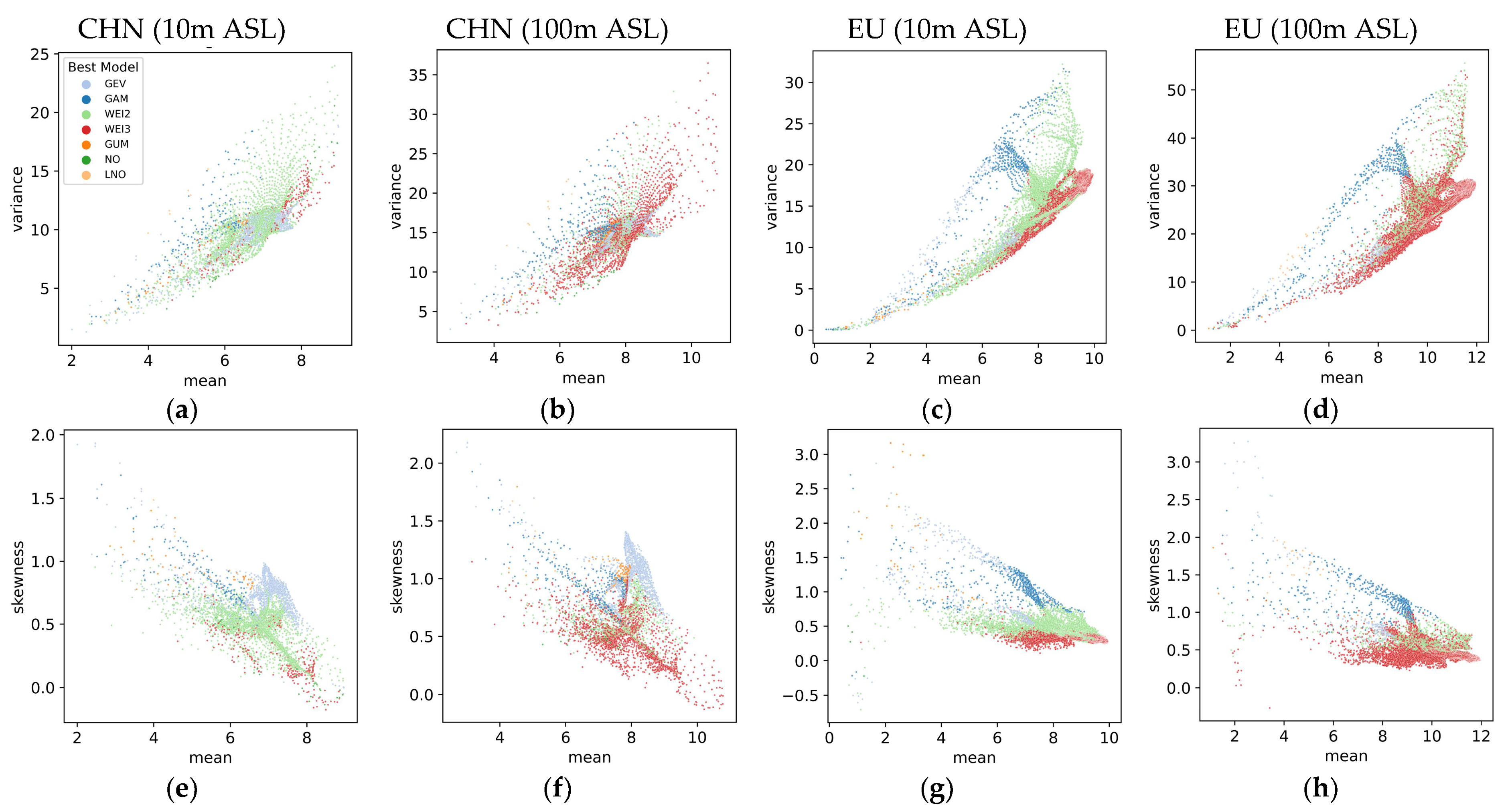
• Model selection based on wind speed characteristics.

For regions with moderate skewness and kurtosis, particularly in the European offshore areas, the Weibull-class models (WEI2 and WEI3) are recommended due to their simplicity and effectiveness.

In areas with higher variability and extreme wind events, such as the East China Sea and the adjacent western Pacific, the Generalized Extreme Value (GEV) model is suggested for its ability to capture extreme values effectively. For regions exhibiting positively skewed wind speed distributions and significant variability, such as the eastern Greenland seas, the Gamma (GAM) distribution model is advised.

2.

Consideration of altitude in model application.

At 10 m ASL, the performance of WEI2 slightly surpasses WEI3 in Chinese coastal areas, while at 100 m ASL, WEI3 shows better performance, indicating the importance of altitude in model selection. In the European seas, the WEI-class models perform consistently well at both altitudes, reflecting the stability of wind conditions.

3.

Importance of skewness and kurtosis.

Skewness is identified as the most significant factor influencing model selection, emphasizing the need to model right-skewed distributions, especially in regions with occasional high wind speed events. Kurtosis also plays a crucial role, particularly in areas with frequent extreme wind events, indicating the occurrence of more frequent extreme wind events.

4.

Regional variability and model flexibility.

The complex variability in wind speeds in the Chinese coastal areas necessitates a more flexible modeling approach compared to the more uniform wind conditions in Europe, where simpler models, like WEI-class models, can be effectively applied.

5.

Future research directions.

Future studies should explore the integration of machine learning techniques and hybrid models to better capture complex wind patterns and enhance model accuracy. The long-term performance and adaptability of these models under changing climate conditions also need to be assessed.

4. Conclusions

This research compares offshore wind resources and optimal wind speed distribution models in China and Europe. It provides insights into the distinct characteristics of wind resources in each region, as well as the applicability of various models. By evaluating widely used wind speed probability distribution (WSPD) models, this study highlights the importance of considering regional wind characteristics in model selection.

• Original research contributions.

This study systematically compares offshore wind resources in China and Europe, revealing significant differences in wind speed characteristics influenced by regional meteorological conditions. The analysis of seven unimodal WSPD models demonstrates that the Weibull distribution is generally the most accurate for wind speed fitting, while the Generalized Extreme Value (GEV) and Gamma distributions perform better in regions with higher skewness and extreme wind events. Additionally, the use of machine learning techniques to evaluate feature importance identifies skewness and kurtosis as critical factors influencing model selection. These findings provide practical guidelines for selecting appropriate models based on regional wind characteristics and altitude, contributing to more accurate offshore wind resource assessments.

2.

Positive aspects.

Using a robust 20-year ERA5 dataset, this study employs multiple evaluation metrics (R², RMSE, AIC, BIC) to ensure a comprehensive and reliable analysis of model performance. The integration of machine learning techniques adds a novel dimension to traditional wind speed modeling by identifying key factors influencing model selection. This research also offers actionable recommendations for model selection based on regional characteristics, supporting decision-making in offshore wind energy assessments. These strengths collectively enhance the practical applicability of this study’s findings.

3.

Observed deficiencies and suggestions for improvement.

While this study provides valuable insights, it relies solely on historical data, which may not fully capture future climate change impacts on wind resources. Additionally, the focus on unimodal models limits the ability to capture multimodal wind speed distributions observed in some regions, particularly in China’s coastal areas. The recommendations provided are based on broad regional characteristics and may not address local-scale variations in wind patterns. Future research should incorporate climate projections to assess the long-term adaptability of the evaluated models. Exploring advanced techniques, such as machine learning algorithms and hybrid models, could improve model flexibility and accuracy, especially in regions with complex wind conditions. Conducting site-specific analyses would further refine model selection and provide more tailored guidance for offshore wind farm planning.

References

1. Jung, C.; Sander, L.; Schindler, D. Future global offshore wind energy under climate change and advanced wind turbine technology. Energy Convers. Manag. 2024, 321, 119075. [Google Scholar] [CrossRef]
2. Meng, D.; Yang, H.; Yang, S.; Zhang, Y.; De Jesus, A.M.P.; Correia, J.; Fazeres-Ferradosa, T.; Macek, W.; Branco, R.; Zhu, S.-P. Kriging-assisted hybrid reliability design and optimization of offshore wind turbine support structure based on a portfolio allocation strategy. Ocean Eng. 2024, 295, 116842. [Google Scholar] [CrossRef]
3. Meng, D.; Yang, S.; Yang, H.; De Jesus, A.M.P.; Correia, J.; Zhu, S.-P. Intelligent-inspired framework for fatigue reliability evaluation of offshore wind turbine support structures under hybrid uncertainty. Ocean Eng. 2024, 307, 118213. [Google Scholar] [CrossRef]
4. Meng, D.; Yang, S.; De Jesus, A.M.P.; Fazeres-Ferradosa, T.; Zhu, S.-P. A novel hybrid adaptive Kriging and water cycle algorithm for reliability-based design and optimization strategy: Application in offshore wind turbine monopile. Comput. Methods Appl. Mech. Eng. 2023, 412, 116083. [Google Scholar] [CrossRef]
5. Akhtar, N.; Geyer, B.; Schrum, C. Larger wind turbines as a solution to reduce environmental impacts. Sci. Rep. 2024, 14, 6608. [Google Scholar] [CrossRef]
6. Sherman, P.; Chen, X.; McElroy, M. Offshore wind: An opportunity for cost-competitive decarbonization of China’s energy economy. Sci. Adv. 2020, 6, eaax9571. [Google Scholar] [CrossRef]
7. Guo, X.; Chen, X.; Chen, X.; Sherman, P.; Wen, J.; McElroy, M. Grid integration feasibility and investment planning of offshore wind power under carbon-neutral transition in China. Nat. Commun. 2023, 14, 2447. [Google Scholar] [CrossRef]
8. Beiter, P.; Mai, T.; Mowers, M.; Bistline, J. Expanded modelling scenarios to understand the role of offshore wind in decarbonizing the United States. Nat. Energy 2023, 8, 1240–1249. [Google Scholar] [CrossRef]
9. Ning, Y.; Wang, L.; Yu, X.; Li, J. Recent development in the decarbonization of marine and offshore engineering systems. Ocean Eng. 2023, 280, 114883. [Google Scholar] [CrossRef]
10. von Krauland, A.K.; Long, Q.; Enevoldsen, P.; Jacobson, M.Z. United States offshore wind energy atlas: Availability, potential, and economic insights based on wind speeds at different altitudes and thresholds and policy-informed exclusions. Energy Convers. Manag. X 2023, 20, 100410. [Google Scholar] [CrossRef]
11. Costoya, X.; deCastro, M.; Carvalho, D.; Feng, Z.; Gómez-Gesteira, M. Climate change impacts on the future offshore wind energy resource in China. Renew. Energy 2021, 175, 731–747. [Google Scholar] [CrossRef]
12. Liu, Y.; Chen, D.; Li, S.; Chan, P.W. Discerning the spatial variations in offshore wind resources along the coast of China via dynamic downscaling. Energy 2018, 160, 582–596. [Google Scholar] [CrossRef]
13. Hasager, C.B.; Hahmann, A.N.; Ahsbahs, T.; Karagali, I.; Sile, T.; Badger, M.; Mann, J. Europe’s offshore winds assessed with synthetic aperture radar, ASCAT and WRF. Wind Energy Sci. 2020, 5, 375–390. [Google Scholar] [CrossRef]
14. Cheynet, E.; Li, L.; Jiang, Z. Metocean conditions at two Norwegian sites for development of offshore wind farms. Renew. Energy 2024, 224, 120184. [Google Scholar] [CrossRef]
15. Gualtieri, G. Analysing the uncertainties of reanalysis data used for wind resource assessment: A critical review. Renew. Sustain. Energy Rev. 2022, 167, 112741. [Google Scholar] [CrossRef]
16. Carvalho, D.; Rocha, A.; Gómez-Gesteira, M.; Santos, C.S. Offshore wind energy resource simulation forced by different reanalyses: Comparisn with observed data in the Iberian Peninsula. Appl. Energy 2014, 134, 57–64. [Google Scholar] [CrossRef]
17. West, C.G.; Smith, R.B. Global patterns of offshore wind variability. Wind Energy 2021, 24, 1466–1481. [Google Scholar] [CrossRef]
18. Shi, H.; Dong, Z.; Xiao, N.; Huang, Q. Wind speed distributions used in wind energy assessment: A review. Front. Energy Res. 2021, 9, 769920. [Google Scholar] [CrossRef]
19. Morales, J.M.; Mínguez, R.; Conejo, A.J. A methodology to generate statistically dependent wind speed scenarios. Appl. Energy 2010, 87, 843–855. [Google Scholar] [CrossRef]
20. Katikas, L.; Dimitriadis, P.; Koutsoyiannis, D.; Kontos, T.; Kyriakidis, P. A stochastic simulation scheme for the long-term persistence, heavytailed and double periodic behavior of observational and reanalysis wind time-series. Appl. Energy 2021, 295, 116873. [Google Scholar] [CrossRef]
21. Carta, J.A.; Ramírez, P.; Bueno, C. A joint probability density function of wind speed and direction for wind energy analysis. Energy Convers. Manag. 2008, 49, 1309–1320. [Google Scholar] [CrossRef]
22. Huang, G.; Jiang, Y.; Peng, L.; Solari, G.; Liao, H.; Li, M. Characteristics of intense winds in mountain area based on field measurement: Focusing on thunderstorm winds. J. Wind. Eng. Ind. Aerodyn. 2019, 190, 166–182. [Google Scholar] [CrossRef]
23. Wang, H.; Xiao, T.; Gou, H.; Pu, Q.; Bao, Y. Joint distribution of wind speed and direction over complex terrains based on nonparametric copula models. J. Wind. Eng. Ind. Aerodyn. 2023, 241, 105509. [Google Scholar] [CrossRef]
24. Huang, S.; Li, Q.; Shu, Z.; Chan, P.W. Copula-based joint distribution analysis of wind speed and wind direction: Wind energy development for Hong Kong. Wind Energy 2023, 26, 900–922. [Google Scholar] [CrossRef]
25. Weibull, W. A statistical distribution function of wide applicability. J. Appl. Mech. 1951, 18, 293–297. [Google Scholar] [CrossRef]
26. Torrielli, A.; Repetto, M.P.; Solari, G. Extreme wind speeds from long-term synthetic records. J. Wind. Eng. Ind. Aerodyn. 2013, 115, 22–38. [Google Scholar] [CrossRef]
27. Jung, C.; Schindler, D. Global comparison of the goodness-of-fit of wind speed distributions. Energy Convers. Manag. 2017, 133, 216–234. [Google Scholar] [CrossRef]
28. Hossain, J.; Sharma, S.; Kishore, V.V.N. Multi-peak Gaussian fit applicability to wind speed distribution. Renew. Sust. Energy Rev. 2014, 34, 483–490. [Google Scholar] [CrossRef]
29. Parzen, E. On estimation of a probability density function and mode. Ann. Math. Stat. 1962, 33, 1065–1076. [Google Scholar] [CrossRef]
30. Han, Q.; Ma, S.; Wang, T.; Chu, F. Kernel density estimation model for wind speed probability distribution with applicability to wind energy assessment in China. Renew. Sustain. Energy Rev. 2019, 115, 109387. [Google Scholar] [CrossRef]
31. Shannon, C.E. A mathematical theory of communication. Bell Syst. Tech. J. 1948, 27, 379–423. [Google Scholar] [CrossRef]
32. Zhang, H.; Yu, Y.-J.; Liu, Z.-Y. Study on the Maximum Entropy Principle applied to the annual wind speed probability distribution: A case study for observations of intertidal zone anemometer towers of Rudong in East China Sea. Appl. Energy 2014, 114, 931–938. [Google Scholar] [CrossRef]
33. Wais, P. A review of Weibull functions in wind sector. Renew. Sustain. Energy Rev. 2017, 70, 1099–1107. [Google Scholar] [CrossRef]
34. IEC 61400-1:2019; Wind Energy Generation Systems—Part 1: Design Requirements. International Electrotechnical Commission: Geneva, Switzerland, 2019.
35. Tenreiro, C. Fourier series-based direct plug-in bandwidth selectors for Kernel Density Estimation. J. Nonparametr. Stat. 2011, 23, 533–545. [Google Scholar] [CrossRef]
36. Kantar, Y.M.; Usta, I. Analysis of the upper-truncated Weibull distribution for wind speed. Energy Convers. Manag. 2015, 96, 81–88. [Google Scholar] [CrossRef]
37. Wais, P. Two and three-parameter Weibull distribution in available wind power analysis. Renew. Energy 2017, 103, 15–29. [Google Scholar] [CrossRef]
38. Hersbach, H.; Bell, B.; Berrisford, P.; Hirahara, S.; Horányi, A.; Muñoz-Sabater, J.; Nicolas, J.; Peubey, C.; Radu, R.; Schepers, D.; et al. The ERA5 global reanalysis. Q. J. R. Meteorol. Soc. 2020, 146, 1999–2049. [Google Scholar] [CrossRef]
39. Olauson, J. ERA5: The new champion of wind power modelling? Renew. Energy 2018, 126, 322–331. [Google Scholar] [CrossRef]
40. Gualtieri, G. Reliability of ERA5 reanalysis data for wind resource assessment: A comparison against tall towers. Energies 2021, 14, 4169. [Google Scholar] [CrossRef]
41. Soares, P.M.M.; Lima, D.C.A.; Nogueira, M. Global offshore wind energy resources using the new ERA-5 reanalysis. Environ. Res. Lett. 2020, 15, 1040a2. [Google Scholar] [CrossRef]
42. Wu, L.; Su, H.; Zeng, X.; Posselt, D.J.; Wong, S.; Chen, S.; Stoffelen, A. Uncertainty of atmospheric winds in three widely used global reanalysis datasets. J. Appl. Meteorol. Clim. 2024, 63, 165–180. [Google Scholar] [CrossRef]
43. Jiang, B.; Hou, E.; Gao, Z.; Ding, J.; Fang, Y.; Khan, S.S.; Wu, G.; Wang, Q.; Meng, F.; Li, Y.; et al. Resource assessment for combined offshore wind and wave energy in China. Sci. China Technol. Sci. 2023, 66, 2530–2548. [Google Scholar] [CrossRef]
44. Zheng, C.; Li, X.; Azorin-Molina, C.; Li, C.; Wang, Q.; Xiao, Z.; Yang, S.; Chen, X.; Zhan, C. Global trends in oceanic wind speed, wind-sea, swell, and mixed wave heights. Appl. Energy 2022, 321, 119327. [Google Scholar] [CrossRef]
45. Feng, X.; Chen, X. Feasibility of ERA5 reanalysis wind dataset on wave simulation for the western inner-shelf of Yellow Sea. Ocean Eng. 2021, 236, 109413. [Google Scholar] [CrossRef]
46. Hayes, L.; Stocks, M.; Blakers, A. Accurate long-term power generation model for offshore wind farms in Europe using ERA5 reanalysis. Energy 2021, 229, 120603. [Google Scholar] [CrossRef]
47. Molina, M.O.; Gutiérrez, C.; Sánchez, E. Comparison of ERA5 surface wind speed climatologies over Europe with observations from the HadISD dataset. Int. J. Climatol. 2021, 41, 4864–4878. [Google Scholar] [CrossRef]
48. MathWorks. atan2d, MATLAB R2024a. Available online: https://www.mathworks.com/help/matlab/ref/atan2d.html (accessed on 21 January 2025).
49. Karin, T. Global Land Mask, Version 1.0.0. PyPI. Available online: https://pypi.org/project/global-land-mask/ (accessed on 21 January 2025).
50. National Centers for Environmental Information (NCEI), NOAA ETOPO1 Data Set, National Oceanic and Atmospheric Administration. Available online: https://www.ngdc.noaa.gov/mgg/global/global.html (accessed on 21 January 2025).
51. Huang, W.; Zhu, X.; Xia, H.; Wu, K. Offshore Wind Energy Assessment with a clustering approach to mixture model parameter estimation. J. Mar. Sci. Eng. 2023, 11, 2060. [Google Scholar] [CrossRef]
52. Wang, J.; Hu, J.; Ma, K. Wind speed probability distribution estimation and wind energy assessment. Renew. Sustain. Energy Rev. 2016, 60, 881–899. [Google Scholar] [CrossRef]
53. Virtanen, P.; Gommers, R.; Oliphant, T.E.; Haberland, M.; Reddy, T.; Cournapeau, D.; Burovski, E.; Peterson, P.; Weckesser, W.; Bright, J.; et al. SciPy 1.0 Contributors. SciPy 1.0: Fundamental algorithms for scientific computing in Python. Nat. Methods 2020, 17, 261–272. [Google Scholar] [CrossRef]
54. Gunturu, U.B.; Schlosser, C.A. Characterization of wind power resource in the United States. Atmos. Chem. Phys. 2012, 12, 9687–9702. [Google Scholar] [CrossRef]
55. Zheng, C. Temporal-spatial characteristics dataset of offshore wind energy resource for the 21st Century Maritime Silk Road. China Sci. Data 2020, 5, 102–115. [Google Scholar] [CrossRef]
56. Ren, G.; Wan, J.; Liu, J.; Yu, D. Characterization of wind resource in China from a new perspective. Energy 2019, 167, 994–1010. [Google Scholar] [CrossRef]
57. Wen, Y.; Kamranzad, B.; Lin, P. Assessment of long-term offshore wind energy potential in the south and southeast coasts of China based on a 55-year dataset. Energy 2021, 224, 120225. [Google Scholar] [CrossRef]
58. Zheng, C.; Pan, J.; Li, J. Assessing the China Sea wind energy and wave energy resources from 1988 to 2009. Ocean Eng. 2013, 65, 39–48. [Google Scholar] [CrossRef]
59. Wilks, D.S. Statistical Methods in the Atmospheric Sciences, 3rd ed.; Elsevier: Oxford, UK, 2011; pp. 125–128. [Google Scholar]
60. Masseran, N.; Razali, A.M.; Ibrahim, K. An analysis of wind power density derived from several wind speed density functions: The regional assessment on wind power in Malaysia. Renew. Sustain. Energy Rev. 2012, 16, 6476–6487. [Google Scholar] [CrossRef]
61. Akaike, H. A new look at the statistical model identification. IEEE Trans. Autom. Control 1974, 19, 716–723. [Google Scholar] [CrossRef]
62. Schwarz, G. Estimating the dimension of a model. Ann. Stat. 1978, 6, 461–464. [Google Scholar] [CrossRef]
63. Breiman, L. Random forests. Mach. Learn. 2001, 45, 5–32. [Google Scholar] [CrossRef]
64. Krzywinski, M.; Altman, N. Classification and regression trees. Nat. Methods 2017, 14, 757–758. [Google Scholar] [CrossRef]
65. Chen, T.; Guestrin, C. XGBoost: A scalable tree boosting system. In Proceedings of the 22nd ACM SIGKDD International Conference on Knowledge Discovery and Data Mining, San Francisco, CA, USA, 13–17 August 2016. [Google Scholar]
66. Fisher, A.; Rudin, C.; Dominici, F. All Models are Wrong, but Many are Useful: Learning a Variable’s Importance by Studying an Entire Class of Prediction Models Simultaneously. J. Mach. Learn. Res. 2019, 20, 177. [Google Scholar]
67. Hughes, M.; Cassano, J.J. The climatological distribution of extreme Arctic winds and implications for ocean and sea ice processes. J. Geophys. Res. Atmos. 2015, 120, 7358–7377. [Google Scholar] [CrossRef]
68. Gorter, W.; van Angelen, J.H.; Lenaerts, J.T.M.; van den Broeke, M.R. Present and future near-surface wind climate of Greenland from high resolution regional climate modelling. Clim. Dyn. 2014, 42, 1595–1611. [Google Scholar] [CrossRef]
69. Laurila, T.K.; Sinclair, V.A.; Gregow, H. Climatology, variability, and trends in near-surface wind speeds over the North Atlantic and Europe during 1979–2018 based on ERA5. Int. J. Climatol. 2021, 41, 2253–2278. [Google Scholar] [CrossRef]
70. Ngo, T.; Letchford, C. A comparison of topographic effects on gust wind speed. J. Wind. Eng. Ind. Aerodyn. 2008, 96, 2273–2293. [Google Scholar] [CrossRef]
71. Pei, C.; Zhang, X.; Cheng, X.; Yang, X.; Ma, C. Impact of different terrains on the distribution of wind pressure on airport terminal roofs in mountainous areas. Structures 2024, 69, 107265. [Google Scholar] [CrossRef]
Figure 1. Annual variations in WPD at 10 m ASL from 2004 to 2023: (a) Chinese sea areas; (b) European sea areas.
Energies 18 01108 g001
Figure 2. Boxplots of R2 and RMSE related to 7 WSPD models for offshore grid cells: (a) R2 of Chinese sea areas; (b) RMSE of Chinese sea areas; (c) R2 of European sea areas; (d) RMSE of European sea areas.
Energies 18 01108 g002
Figure 3. Distributions of nearshore points (blue) and offshore points (red): (a) Chinese sea areas; (b) European sea areas.
Energies 18 01108 g003
Figure 4. The distribution of the overall scores of WSPD models: (a) R2 of Chinese sea areas; (b) RMSE of Chinese sea areas; (c) R2 of European sea areas; (d) RMSE of European sea areas.
Energies 18 01108 g004
Figure 5. Frequency distribution of optimal and suboptimal models across (a) Chinese sea areas and (b) European sea areas. Note: Darker colors indicate the proportions of optimal models, while lighter shades represent the proportions of suboptimal models.
Energies 18 01108 g005
Figure 6. The distribution of the optimal WSPD models: (a) Chinese sea areas at 10 m ASL; (b) Chinese sea areas at 100 m ASL; (c) European sea areas at 10 m ASL; (d) European sea areas at 100 m ASL. ‘WS’ refers to ‘wind speed’.
Energies 18 01108 g006
Figure 7. The distribution of the suboptimal WSPD models: (a) Chinese sea areas at 10 m ASL; (b) Chinese sea areas at 100 m ASL; (c) European sea areas at 10 m ASL; (d) European sea areas at 100 m ASL. ‘WS’ refers to ‘wind speed’.
Energies 18 01108 g007
Figure 8. Distribution of wind speed characteristics across Chinese sea areas at (ad) 10 m ASL and (eh) 100 m ASL. ‘ws’ refers to ‘wind speed’.
Energies 18 01108 g008
Figure 9. Distribution of wind speed characteristics across European sea areas at (ad) 10 m ASL and (eh) 100 m ASL. ‘ws’ refers to ‘wind speed’.
Energies 18 01108 g009
Figure 10. Scatter plots showing the correlations between pairs of wind speed characteristics at 10 m ASL (a,e,i,m,q,u) and 100 m ASL (b,f,j,n,r,v) for Chinese seas and at 10 m ASL (c,g,k,o,s,w) and 100 m ASL (d,h,l,p,t,x) for European seas.
Energies 18 01108 g010aEnergies 18 01108 g010b