Research on Reliability Improvement Method of Mountainous Power Grid Considering Electrified Railways Access

Abstract

The mountainous power grids exhibit significantly lower reliability compared to conventional urban grids due to inherent structural weaknesses, dispersed load distribution, and higher failure probabilities of power supply equipment. With the ongoing construction and commissioning of electrified railways in western China, it is crucial to analyze the impact of strong shocks and random fluctuations in traction loads on mountainous power grids, and to study the reliability enhancement of these grids considering electrified railways access, to ensure their safety and the reliable, continuous power supply for the railways. Therefore, this paper proposes a method to enhance the reliability of mountainous power grids considering electrified railways access. First, stochastic fluctuation characteristics of traction loads are simulated through train traction calculations. Subsequently, the reliability level of mountainous grids is quantitatively evaluated, with a novel line vulnerability index established to identify weak grid sections. Finally, two complementary enhancement strategies are proposed: dynamic line capacity expansion and optimized backup capacity allocation. Case studies demonstrate the effectiveness of the method through comparative analysis of reliability indices before and after implementation, confirming both technical validity and practical feasibility.

1. Introduction

A series of representative 200 km/h passenger and freight railways, such as the Sichuan–Tibet Railway and the Yunnan–Tibet Railway, will be successively built in China, which will significantly increase the proportion of electrified railway loads in mountainous power grids. A mountainous power grid refers to the power distribution system located in mountainous areas, which mainly serves the electricity demand in mountainous areas. To meet the traction power demands of electric locomotives under long steep gradients and tunnels in the western mountainous regions, the traction power supply system of electrified railways in these areas requires strong and reliable support from the external power grid. However, unlike ordinary urban power grids, the reliability of the power supply in mountainous area grids is relatively low due to the constraints imposed by the mountainous terrain: (1) Since most mountainous area grids are exposed in open-air regions with harsh natural environments, power supply equipment is highly susceptible to aging. Once a fault occurs, grassroots repair personnel are unable to reach the site in a timely manner to carry out maintenance and repair work, resulting in untimely maintenance of power supply equipment; (2) Limited by the complex geographical and geological conditions, there are fewer high-voltage substations in mountainous areas, and the grid structure is relatively weak. Additionally, the dispersed distribution of electricity consumers in mountainous areas leads to a large power supply coverage area, which reduces the reliability of the power supply in mountainous area grids [1,2]; (3) With the continuous construction of electrified railways operating under mixed passenger and freight conditions in mountainous area grids, the integration of large-scale, high-impact, and randomly fluctuating traction loads will affect the reliability of the mountainous area grids. This, in turn, exposes electrified railways to the risk of an unreliable external power supply. The harsh transportation conditions along the railway lines pose a certain threat to the safe and reliable operation of electrified railways. Therefore, there is an urgent need to strengthen the upgrading and renovation of the power grid in the western mountainous regions and to research reliability enhancement solutions for these grids.

In the power grid, the transmission capacity of transmission lines is a critical electrical parameter, as its magnitude constrains the overall system’s transmission capability and consequently affects the reliability level of the grid [3]. When high-power, strong-impact traction loads are connected to the power grid, the injected power at the grid nodes fluctuates with the movement of the trains, causing a redistribution of the line flow. When the transmission capacity of the lines is insufficient, this redistributed flow can easily exceed the transmission limits, leading to a decline in line reliability parameters and potentially causing the lines to fail or disconnect due to overload. Therefore, it is crucial to properly expand the key lines of the power grid to reduce the impact of electrified railway traction loads’ access on the reliability parameters of the grid lines.

Additionally, the access of traction loads increases the uncertainty in the power grid, raising higher demands on the adjustment capabilities and standby capacity of the grid’s generating units. Therefore, in improving grid reliability, most literature has focused extensively on methods to enhance reliability from the perspectives of transmission line dynamic expansion and unit standby capacity configuration.

Transmission line dynamic expansion can fully exploit the transmission potential of the power grid, providing greater margins for reliable grid operation [4,5,6]. Relevant research mainly focuses on two aspects: the impact of transmission line dynamic expansion on load reduction at grid nodes [4,7] and the effect on overall grid reliability [8,9]. For example, ref. [7] indicates that since the DTR model of transmission lines considers temperature variations, the thermal inertia and short-term overload limits of transmission lines can effectively reduce the load shedding at relevant grid nodes in the short period following a generator or other component failure. Ref. [4] introduces the concept of grid flexibility and proposes a flexible optimal load-shedding strategy considering the DTR. It analyzes the impact of considering the DTR of the transmission line on the total load shedding and the incremental system risk. This research focuses on the overall reliability of the grid as influenced by the dynamic expansion of transmission lines. Ref. [8] considers the real-time transmission capacity of transmission lines under different weather conditions and uses the Monte Carlo simulation method to assess the reliability levels of the IEEE 14-bus, 24-bus, and 39-bus test systems. The study verifies the significant enhancement of grid reliability levels through dynamic line expansion. Ref. [9] considers the impact of grid generation uncertainty on the system and investigates the impact of the transmission line DTR on grid reliability based on the improved IEEE RTS-79 bus test system. The results indicate that incorporating a DTR improves the reliability level of the power grid. Ref. [10] proposes an optimal real-time transmission congestion management algorithm for power grids. By considering the dynamic capacity of transmission lines, it calculates the potential transmission capability and uses an optimal load-shedding strategy to effectively mitigate transmission congestion issues during grid operation, thereby reducing the total load shedding in the power grid.

When a power grid fault occurs, operating reserves can ensure the continuous and effective power supply to loads, thereby guaranteeing the safe and reliable operation of the power grid. Currently, existing research on power grid reserve capacity configuration is mainly divided into two categories: the deterministic method and the probabilistic method.

(1)

The widely used deterministic methods determine reserve capacity based on the maximum unit capacity within the system (N-1 method), a fixed percentage of peak load in the system, and so on. For example, the Guide on Technology for Power System in China [11] specifies that reserve capacity for power system loads is generally set at 2% to 5% of the maximum generation load, with complex large systems typically set at 2% and smaller systems at 5%. Generally, power grid companies in China use deterministic methods to determine the reserve capacity required for the actual operation of the power grid. For example, the China Southern Power Grid stipulates that the reserve capacity for the entire network should be no less than 2% of the maximum load, while the contingency reserve should be 8% to 12% of the maximum load [12]. The Central China Grid sets the load reserve and contingency reserve at 2% and 5% of the system’s maximum load, respectively [13]. The East China Grid determines its reserve capacity as the sum of the maximum bipolar transmission power in actual grid operation and the capacity of the largest single unit [14].

(2)

Deterministic methods are simple in principle and convenient to calculate. However, they do not consider factors such as generator outages and load fluctuations within the power grid, which can lead to insufficient or wasted reserve capacity, threatening system reliability or economic efficiency. Probabilistic methods take into account the probabilistic characteristics of various uncertainties in the power grid, such as generator capacity and load levels. They comprehensively evaluate the overall reliability of the system from the perspective of reserve capacity. By setting specific reliability indices, these methods optimize the configuration of reserve capacity within the system [15]. Ref. [16] incorporates the limit of the reliability index known as the expected power deficiency as a constraint into the optimization scheduling model of the power system. Refs. [17,18] study the impact of uncertainty factors on reserve capacity in power systems using chance-constrained methods, based on the probability distribution functions of generator output and load forecast errors. Ref. [19] simultaneously considers the probability of grid incidents and the potential economic losses resulting from such incidents. By incorporating loss risk into the objective function, it optimizes the system’s reserve configuration scheme.

As a high-power, high-impact mobile load, the large-scale integration of electrified railway traction loads into the power grid will cause a rapid redistribution of system flow, altering the operational state of the system and affecting grid reliability. However, existing work primarily focuses on improving grid reliability after the integration of distributed generation sources like wind power [20,21,22], with relatively less research dedicated to enhancing grid reliability following the integration of traction loads.

In summary, as electrified railways progressively expand into the western mountainous regions, there is an urgent need to conduct research on the power supply reliability of these mountainous power grids. It is essential to comprehensively quantify the impact of electrified railway traction loads on the reliability level of mountainous power grids and accurately assess the overall reliability of the power supply. At the same time, with the increasing number of electrified railways being put into operation in mountainous areas, enhancing the power supply reliability can reduce or even avoid the impact on the reliability of the mountainous area power grid caused by the integration of electrified railways. This is of great significance for achieving a reliable and sustainable power supply in mountainous area grids and ensuring the safe and reliable operation of electrified railways. To ensure that the power grid can still supply power safely and reliably after the integration of electrified railways, this paper considers the impact of traction load, an uncertain factor, during the operation of mountainous area grids. The main contributions of this paper are as follows:

(1)

Analysis of the Impact of Traction Load Characteristics on Mountainous Power Grid Reliability

One of the novel contributions of this paper lies in the detailed analysis of the impact of traction load characteristics on the reliability of mountainous power grids. Previous research on power grid reliability has generally focused on conventional static loads or the integration of distributed generation sources such as wind power. However, these studies have not taken into account the dynamic and high-impact nature of traction loads, particularly from electrified railways. Traction loads exhibit rapid and fluctuating power demands, caused by factors such as acceleration, deceleration, and regenerative braking of trains. These characteristics introduce significant instability into the power grid, especially in mountainous regions where infrastructure is weak and the system’s capacity to handle such fluctuations is limited. This paper fills this gap by explicitly considering how these unique traction load dynamics affect the reliability of mountainous power grids, offering insights that are absent in previous literature.

(2)

Proposed Reliability Enhancement Methods Specifically Tailored for Mountainous Power Grids Under Traction Load Influence

In addition to analyzing the impact of traction loads, this paper also proposes specific reliability enhancement methods tailored for mountainous power grids under the influence of these loads. Unlike previous studies that focus on general grid improvements or neglect the complexities introduced by high-impact dynamic loads, the proposed methods in this paper—such as dynamic expansion of transmission lines and optimal standby capacity configuration—are designed to address the unique challenges posed by fluctuating traction loads. By dynamically adjusting transmission line capacities based on real-time operational data and strategically allocating standby capacity to accommodate these load variations, this paper provides a more targeted approach to enhancing the reliability of mountainous power grids. This consideration of the specific demands of traction loads sets this work apart from existing research, making it a significant contribution to the field of power system reliability in challenging environments.

2. Reliability Assessment of Power Systems in Mountainous Areas Considering Access of Electrified Railways

The same access to the traction load, one of the important differences between mountainous power grids and ordinary power grids, is that “passenger and freight mixing” occurs in mountainous areas, so in view of this situation, this section describes in detail the differences between ordinary power grids and mountainous power grids, as shown in the

Table 1. Mountain grid vs. general grid.

Comparison Term	Mountain Power Grid	General Grid
Electricity supply capacity	Small capacity, low short-circuit capacity	High capacity, high short-circuit capacity
Voltage stability	Load changes are prone to voltage fluctuations	Low impact of load shocks on voltage
Flexibility	Adaptation to small power, stable load	Adaptation to high power, sudden change in load
Affected by freight trains	Higher impact, prone to voltage dips and power quality degradation	Impacts are small and the grid can cope with them through scheduling
Reliability of power supply	Lower reliability due to line length and topography	High stability and reliability of the power supply network

.

The access of traction loads will cause fluctuations in the injected power at grid nodes, leading to a redistribution of the whole network flow and altering the operational state of the grid. To analyze the reliability level of the grid under different operating conditions and identify weak points in grid reliability, it is necessary to conduct a reliability assessment. After considering the access of traction loads, the following reliability indicators are defined to quantitatively analyze the power supply reliability and reliability weaknesses of the mountainous power grid.

Loss of Load Probability (LOLP): The probability of experiencing load shedding within a specified simulation period.

$$LOLP={\displaystyle \frac{N_{\mathrm{loss}}}{N}}$$

(1)

In Equation (1), N is the number of simulation samples, and N_loss is the total number of times load shedding occurs within N simulation samples.

Loss of Load Frequency (LOLF): The frequency of load-shedding occurrences within a specified simulation period.

$$LOLF={\displaystyle \frac{N_{\mathrm{loss}}}{T_{\mathrm{time}}}}$$

(2)

In Equation (2), T_time is the total simulation time.

In the context of power system reliability assessment, Equation (1) Loss of Load Probability (LOLP) and Equation (2) Loss of Load Frequency (LOLF) serve as crucial metrics for evaluating the reliability of the power grid. Their specific interpretations in power system simulations are as follows:

• Equation (1) LOLP (Loss of Load Probability): Load Loss Probability:

In this context, N_loss refers to the total number of occurrences of load loss (i.e., when the power grid is unable to meet the full load demand) during the simulation, while N represents the total number of samples generated throughout the entire simulation process. In power system simulations, this indicator reflects the probability of load loss occurring under specific operating conditions. A higher LOLP value indicates a higher frequency of power supply insufficiency during the simulation, suggesting lower grid reliability. This metric is commonly used to evaluate the grid’s ability to maintain power supply under conditions such as fluctuations in traction load, system faults, or emergency scenarios.

• Equation (2) LOLF (Loss of Load Frequency): Load Loss Frequency:

In this, N_loss still represents the total number of occurrences of load loss, while T_time represents the total duration of the entire simulation. This indicator measures the average number of times the power grid experiences load loss within a given period. Unlike LOLP, LOLF focuses more on the frequency of load loss events rather than just the probability of their occurrence. For example, in mountainous grid systems, if a high-power surge from traction load causes line overloading or voltage drops, the grid may experience multiple short-term power shortages. In this case, the LOLF value would be higher. A higher LOLF value indicates poor power supply reliability, meaning that load loss events occur more frequently, which may have a significant impact on the stable operation of the railway traction system.

In practical power system simulations, these two indicators are often used in combination. For example, in the study of mountainous grid systems, LOLP is mainly used to assess the risk of power shortages, while LOLF can reveal the pattern of load loss over a specific time period, helping to identify critical weak points and develop targeted reliability improvement strategies, such as increasing backup capacity or optimizing the transmission network configuration.

Expected Demand Not Supplied (EDNS): The average amount of load shedding in the power grid within a specified simulation period.

$$EDNS={\displaystyle \frac{{\displaystyle \sum _{i=1}^{T_{\mathrm{time}}}{S}_i}}{T_{\mathrm{time}}}}$$

(3)

In Equation (3), S_i is the total amount of load shedding in the power grid during the ith sampling.

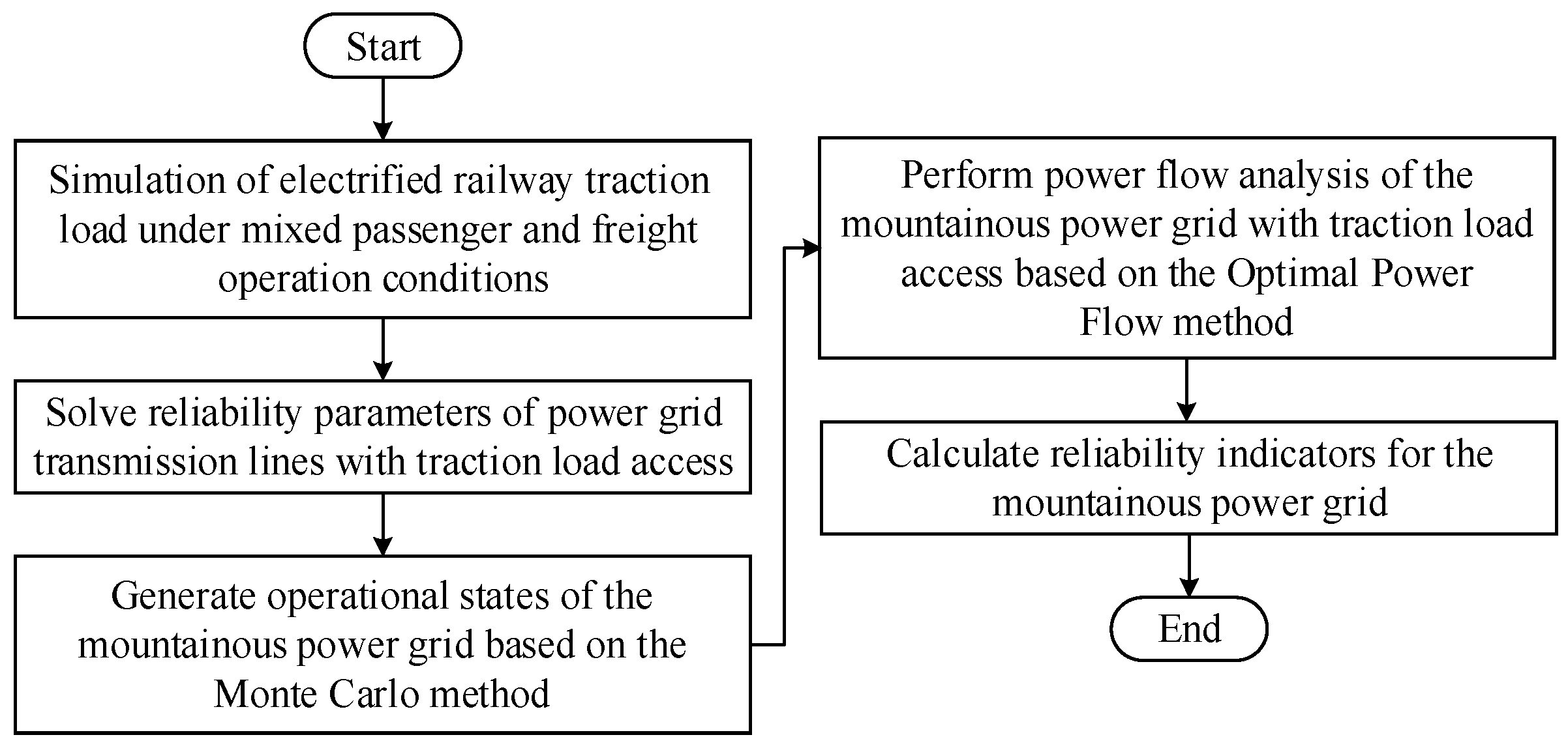
Based on the above evaluation indicators, the Monte Carlo method is used to simulate the system operating states and calculate these indicators. The assessment process is illustrated in Figure 1; the specific steps include the following:

(1)

Establishing the electrified railroad traction load power model under the condition of mixed running of passengers and goods by considering the factors such as line density, locomotive type, and line-driving environment.

(2)

Considering the influence of the high-power fluctuation characteristics of electrified railroad traction load on the power of the grid line, calculate the line failure outage rate.

(3)

According to the fault outage rate of the grid lines, the Monte Carlo method is used to sample the operating state of the grid, and the total number of sampling times is N.

(4)

Analyze the grid operation state based on the optimal tidal current method and record the load shedding of the grid under the current state.

(5)

If the sampling number is greater than the total sampling number, calculate the reliability index, otherwise return to (4).

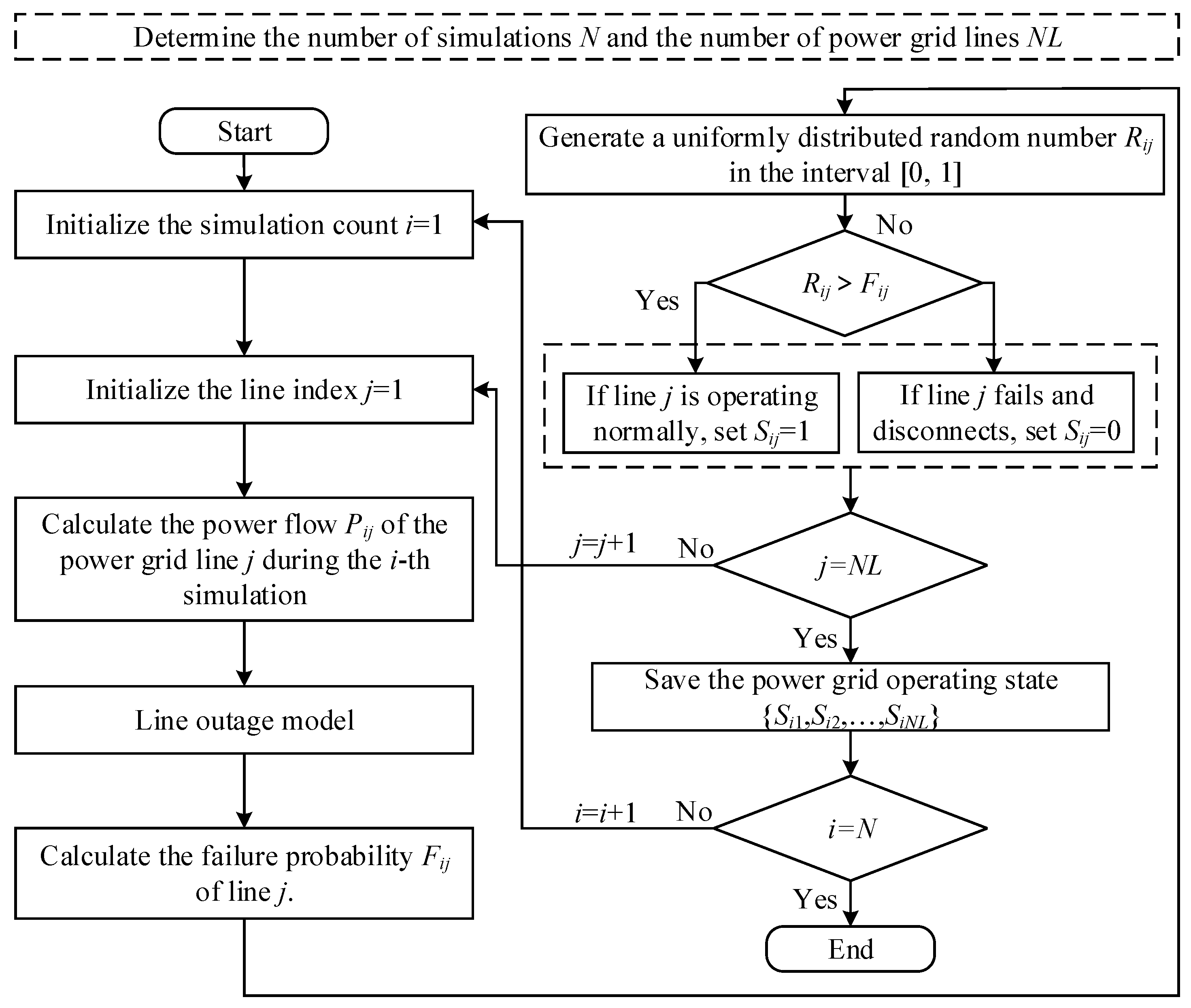
The Monte Carlo method regards the combination of all component states as the state of a system, and the state of each component can be determined by sampling the probability that the component appears in the state: the component has normal and fault states, which can be simulated by a uniformly distributed random number in the [0, 1] interval. When the component failure probability is greater than the random number, it is considered that the component is currently in a fault state. The simulation process of the power grid operation state based on the Monte Carlo method is shown in Figure 2.

3. Reliability Enhancement of Power Systems in Mountainous Areas Considering Access of Electrified Railways

When electrified railways access mountainous power grids, factors such as traction load fluctuations, equipment and line failures, and forced outages of generating units can cause active power shortages in the grid. This can even lead to widespread line outages, affecting the reliability level of the power supply in the grid. To ensure the power grid can still supply power safely and reliably after electrified railway access, reliability enhancement schemes for mountainous power grids are explored from two perspectives: transmission line dynamic expansion and unit standby capacity configuration.

3.1. Reliability Enhancement Method for Power Systems in Mountainous Areas Considering Dynamic Expansion of Transmission Lines

As mentioned above, the transmission capacity of transmission lines restricts the overall transmission capability of the entire power grid. Dynamic expansion of transmission lines can enlarge the search space of the load-shedding solutions in the power flow analysis model to a certain extent, thereby alleviating the problem of power grid load loss caused by large-scale uncertain traction load access.

Transmission line dynamic expansion refers to the following: without changing the original structure of the lines, using real-time monitoring or predicted dynamic meteorological information to apply a line thermal equilibrium model to estimate the transmission capacity limit of the transmission lines in real time. Based on real-time estimates of the transmission capacity of transmission lines over multiple periods, conduct a line expansion analysis to calculate the required expansion capacity for the lines.

This study not only considers the unique load characteristics of mountainous power grids (such as the highly fluctuating traction loads of electrified railways) but also incorporates the effects of complex mountain climate conditions on transmission capacity, leading to targeted improvements in transmission capacity calculations and expansion strategies.

3.1.1. Estimation of Transmission Capacity Limits Based on the Line Thermal Equilibrium Model

At present, both domestic and international standards have established corresponding regulations for the calculation process of dynamic capacity limits for transmission lines [23,24,25]. This paper calculates the dynamic capacity limits of transmission lines based on the widely used IEEE Std. 738 standard [26,27,28]. The line thermal equilibrium model is as follows:

$$P_{\mathrm{DTR}}=P_{\mathrm{c}}+P_{\mathrm{r}}-P_{\mathrm{s}}$$

(4)

In Equation (4), P_DTR is the transmission capacity limit of the line, P_c is the convective heat dissipation of the line, P_r is the solar radiation absorption by the line, and P_s is the radiative heat dissipation of the line.

The line convection heat dissipation P_c is taken as the maximum value in three environments: completely stationary windless P_cn, low wind speed P_c1, and high wind speed P_c2, and the corresponding calculation method is shown in Equations (5)–(7):

$$P_{\mathrm{cn}}=3.645{\rho }_{\mathrm{f}}^{0.5}{D}_{\mathrm{c}}^{0.75}{\left(T_{\mathrm{s}}-T\right)}^{1.25}$$

(5)

$$P_{\mathrm{c}1}=K_{\mathrm{d}}{K}_{\mathrm{f}}\left(T_{\mathrm{s}}-T\right)\left[1.01+1.35{\left({\displaystyle \frac{D_{\mathrm{c}}{\rho }_{\mathrm{f}}v}{{\mu }_{\mathrm{f}}}}\right)}^{0.52}\right]$$

(6)

$$P_{\mathrm{c}2}=0.754K_{\mathrm{d}}{K}_{\mathrm{f}}\left(T_{\mathrm{s}}-T\right){\left({\displaystyle \frac{D_{\mathrm{c}}{\rho }_{\mathrm{f}}v}{{\mu }_{\mathrm{f}}}}\right)}^{0.6}$$

(7)

In Equations (5)–(7), ρ_f is the air density, D_c is the diameter of the line, T_s is the surface temperature of the line, T is the external ambient temperature, K_d is the wind direction factor, K_f is the air thermal conductivity, μ_f is the air viscosity, and v is the external ambient wind speed.

The calculation method for the solar radiation absorption by the line P_r is shown in Equation (8):

$$P_{\mathrm{r}}=17.8D_{\mathrm{c}}\epsilon \left[{\left({\displaystyle \frac{T_{\mathrm{s}}+273}{100}}\right)}^4-{\left({\displaystyle \frac{T+273}{100}}\right)}^4\right]$$

(8)

In Equation (8), ε is the emissivity of the line surface, typically ranging from 0.23 to 0.91.

The calculation method for the radiative heat dissipation of the line P_s is shown in Equation (9):

$$P_{\mathrm{s}}=A\alpha Q_{\mathrm{se}}\sin \left(\theta \right)$$

(9)

In Equation (9), A is the projected area of the line, α is the solar radiation absorption coefficient of the line, typically ranging from 0.23 to 0.91, Q_se is the total solar radiation heat flux density corrected for elevation, and θ is the effective angle of incidence of the solar radiation.

It is important to note that, due to the long length of the transmission lines in actual power grids, which often span multiple meteorological regions, the maximum transmission capacity of the entire line is typically constrained by the capacity limits of the line segments under the most severe meteorological conditions. Therefore, the actual transmission capacity of the line is taken as the minimum value of the transmission capacity extremes from different meteorological regions. The specific calculation method is shown in Equation (10):

$$P_{\lim ,\mathrm{DTR}}=\min \left\{P_{\mathrm{DTR},r}\left|r\in Region\right.\right\}$$

(10)

In Equation (10), P_lim,DTR is the actual transmission capacity limit of the line, P_DTR,r is the transmission capacity limit of the line when passing through meteorological region r, and Region is the set of all meteorological regions the line spans.

3.1.2. Dynamic Expansion Scheme for Transmission Lines in Mountainous Power Systems Considering Dynamic Expansion Capacity

Considering the impact characteristics of traction load fluctuations, which cause short-term power flow fluctuations in the power grid and exacerbate line overload and disconnection, the dynamic expansion capacity C_a of the transmission lines is defined. By reasonably increasing the transmission capacity of critical lines in the power grid, the adverse effects of traction load on mountainous power grids can be mitigated, thereby enhancing the reliability of these power grids. The calculation method for the dynamic expansion capacity of the transmission lines is presented in Equation (11):

$$C{a}_i=\max \left\{P_{\lim ,\mathrm{DTR}}\left(t\right)-P_{\mathrm{L}i}\left(t\right)\left|t\in T\right.\right\}$$

(11)

In Equation (11), Ca_i is the expansion capacity of line i, T is the simulation time, P_lim,DTR(t) is the transmission capacity limit of line i at time t, calculated based on the external dynamic operating environment parameters, and P_Li(t) is the transmission capacity of line i at time t.

The proposed process for dynamic expansion of the transmission lines in mountainous power grids is illustrated in Figure 3, and the specific steps are as follows:

(a)

Obtain external operating environment parameters for all regions crossed by the transmission lines requiring expansion in the mountainous power grid, including temperature, wind speed, and regional latitude;

(b)

Estimate the transmission capacity limit of the line based on the line thermal equilibrium model. Select the minimum value of the transmission capacity extremes from different meteorological regions, as determined by Equation (10), as the actual transmission capacity limit of the line;

(c)

Consider the access of electrified railway traction loads and perform power flow analysis for the mountainous power grid. During real-time train operations, calculate and record the transmission capacity of the transmission lines at each moment;

(d)

Combine the real-time calculation results of line transmission capacity over multiple periods to conduct line expansion analysis. Calculate the required expansion capacity for the lines based on Equation (11).

3.2. Reliability Enhancement Method for Power Systems in Mountainous Areas Considering Unit Standby Capacity Configuration

To address the impact of uncertainties such as the random fluctuations of traction loads on the operation of mountainous power grids, it is necessary to allocate standby capacity for the generators within the grid reasonably to ensure a continuous power supply. However, excessive standby capacity in the grid incurs higher economic costs, while insufficient standby capacity fails to meet the system’s reliability requirements. Therefore, it is essential to study standby capacity allocation schemes for mountainous power grids under the condition of meeting certain reliability requirements.

3.2.1. Optimal Power Flow Model for the Power Grid Based on Standby Capacity

When configuring standby capacity for each generator in the power grid, it is necessary not only to consider the rated capacity and initial active power output of the generators but also to account for the ramp rate constraints of different generators. Therefore, it is essential to improve the optimal power flow model of the grid by adding two additional constraints: the standby capacity configuration constraint and the generator output constraint considering standby capacity. The specifics are as follows:

(1)

Generator standby capacity configuration constraint:

$$0\le {{\displaystyle R}}_i\le \min \left({{\displaystyle P}}_{\mathrm{g}i,\max }-{{\displaystyle P}}_{\mathrm{g}i}^0,10{{\displaystyle r}}_i\right)$$

(12)

(2)

Generator output constraint taking into account standby capacity:

$${{\displaystyle P}}_{\mathrm{g}i}\le {{\displaystyle R}}_i+{{\displaystyle P}}_{\mathrm{g}i}^0$$

(13)

In the equation, R_i is the standby capacity of generator i, $P_{\mathrm{g}i}^0$ is the initial capacity of generator i, r_i is the ramp rate of generator i, and 10 r_i is the capacity that generator i can increase within 10 min.

During the solution process of the optimal power flow model considering standby capacity, it is found that the result of the objective function is dependent on the constraints. Specifically, changes in the standby capacity R of grid generators lead to changes in the grid operation constraints, which in turn cause variations in the load-shedding amount S. According to Equation (3), the mean indicator of power grid reliability load loss EDNS is related to the objective function value S of the optimal power flow model. Therefore, it can be inferred that the grid reliability indicator EDNS varies with changes in the random standby capacity R, and the impact of changes in standby capacity for different generators on grid reliability varies in degree. To measure the extent of change in the grid reliability indicator EDNS caused by variations in generator standby capacity, this paper proposes the reliability contribution index γ based on sensitivity analysis methods. The specific calculation method is as follows:

$${\gamma }_j={\displaystyle \frac{\mathsf{\partial }EDNS}{\mathsf{\partial }{{\displaystyle R}}_i}}={\displaystyle \frac{{\displaystyle \sum _i\frac{\mathsf{\partial }{{\displaystyle S}}_i}{{{\displaystyle R}}_j}}}{{{\displaystyle T}}_{\mathrm{time}}}}$$

(14)

In Equation (14), γ_j is the reliability contribution index of generator j, S_i is the total load-shedding amount in the ith simulation, R_j is the standby capacity of the generator, and T_time is the total number of simulations.

Therefore, if a generator in the power grid has a higher reliability contribution index, the impact of changes in its standby capacity on the grid reliability indicator EDNS is more significant. When enhancing grid reliability, priority can be given to optimizing a standby capacity configuration for generators with higher reliability contribution indices.

3.2.2. Standby Capacity Allocation Scheme for Mountainous Power Systems Considering Reliability Contribution Index

Define the total operational cost of the power grid as consisting of two components: the total cost of power outage losses and the cost of standby capacity allocation. The specific calculation methods are as follows:

$$Cost=\alpha EDNS+\beta {{\displaystyle R}}_{\mathrm{total}}$$

(15)

In Equation (15), α is the unit cost of power outage losses for the grid, β is the unit cost of standby capacity for the grid’s generators, and R_total is the sum of standby capacities for all generators within the grid.

When the total operational cost Cost of the grid is minimized, the derivative of Equation (15) is equal to zero:

$$\alpha \Delta EDNS+\beta {{\displaystyle \Delta R}}_{\mathrm{total}}=0$$

(16)

In Equation (16), ΔEDNS is the increment in the reliability indicator EDNS after increasing the standby capacity by ΔR_total.

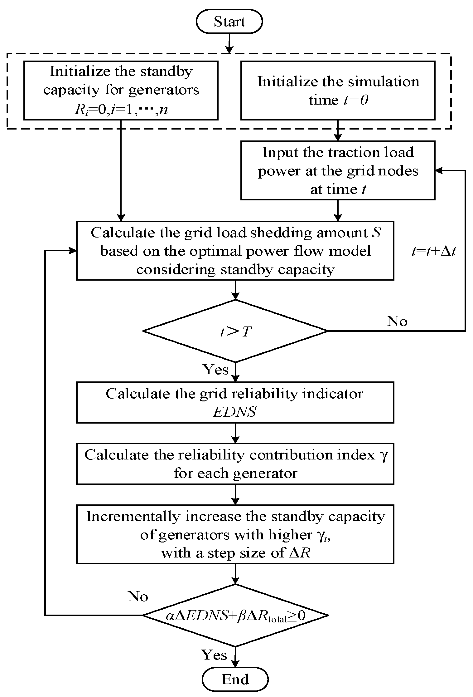
The proposed optimization process for the grid standby capacity configuration is illustrated in Figure 4. The specific steps are as follows:

(a)

Initialize the standby capacity for each generator in the grid with R_i = 0, i = 1, …, n, and initialize the simulation time;

(b)

Input the traction load power at the grid nodes at time t;

(c)

Calculate the load-shedding amount for the mountainous power grid using the optimal power flow model that includes standby capacity. Determine if t > T. If yes, calculate the grid reliability indicator EDNS and the reliability contribution index γ for each generator. Otherwise, repeat step (b);

(d)

Find the generator with the larger reliability contribution γ, and incrementally increase the standby capacity of these generators by a certain step size ΔR;

(e)

Determine whether the iteration stopping condition

αΔEDNS + βΔRtotal ≥ 0 is satisfied. If so, terminate the iteration; otherwise, repeat step (c).

4. Example Analysis

Taking as an example a 200 km/h mixed passenger and freight electrified railway under construction, which will be connected to a power grid in the western mountainous region of China, the proposed method is used for reliability assessment and improvement studies. The simulation time is 24 h, and the traction load power simulation sampling step Δt is 0.01 min.

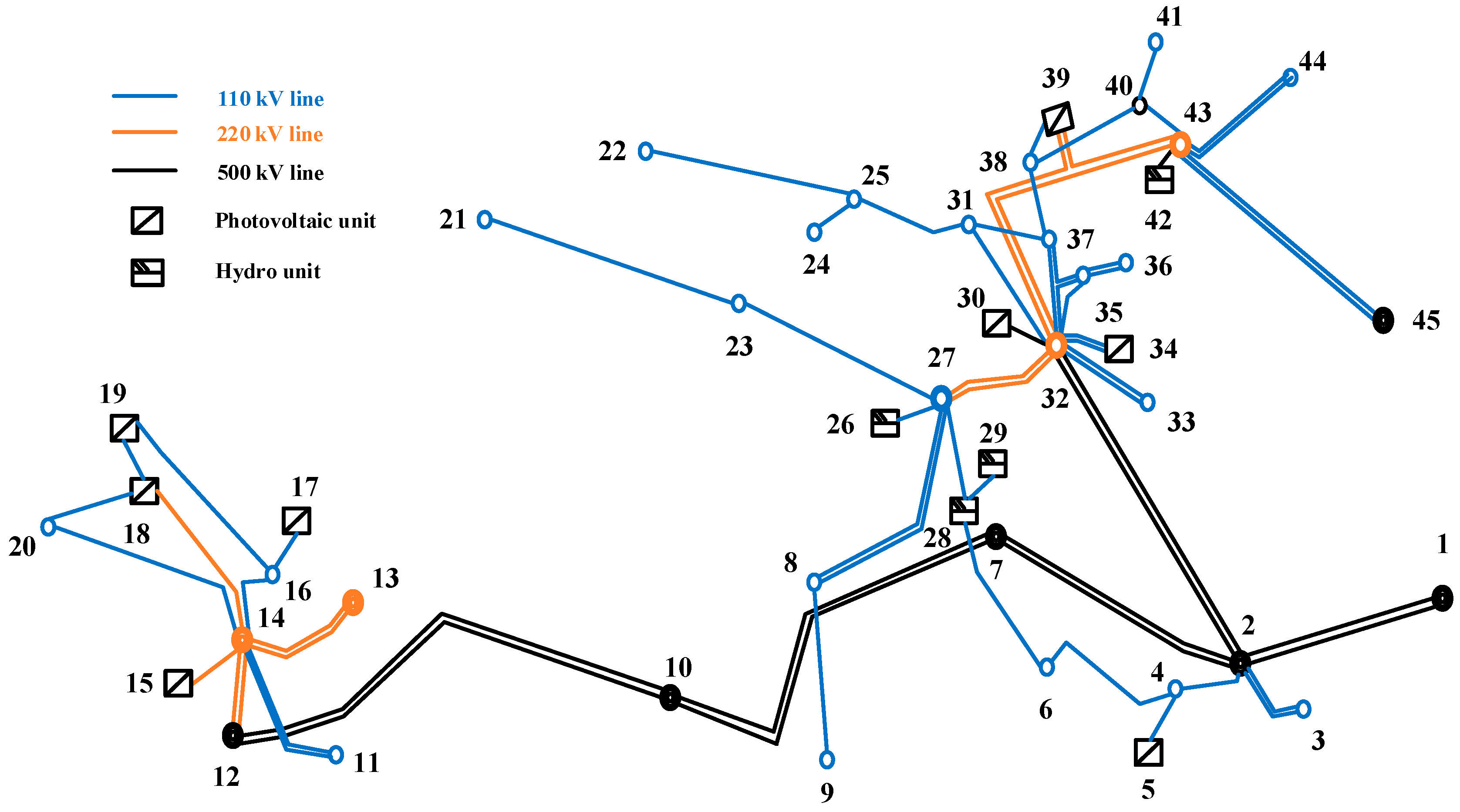
4.1. Mountainous Power Grid Structure

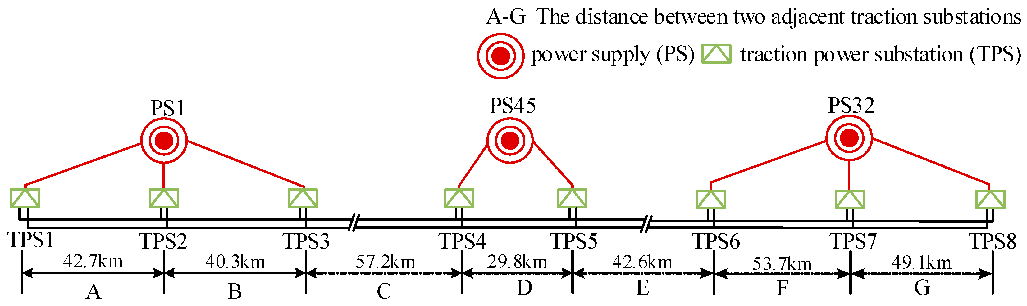
The topology of the western mountainous power grid is shown in Figure 5. The relevant parameters of the mountainous power grid are referenced from the electrified railway traction power supply system planned in the western region of China [29]. Line parameter information is primarily referenced from manuals [30,31], as shown in

Table 2. Power grid transmission line parameter information.

Voltage Level	Wire Model	Unit Reactance/ (Ω·km−1)	Transmission Capacity Limit/MW
110 kV	LGJ-185	0.4	98
220 kV	LGJ-240 × 2	0.3006	200
500 kV	LGJ-4 × 500	0.2975	1000

.

4.2. Mountainous Power Grid Reliability Assessment Result

Based on the electrified railway power supply design scheme and the actual geographical conditions along the railway, the following settings are made:

(1)

The traction power supply system is planned to use a double-sided integrated uninterrupted power supply mode to draw electricity from the external grid, as shown in Figure 6:

(2)

Simultaneously consider the situation where multiple trains are operating in both the up and down directions. Define the up direction as TPS1→TPS8. Assume that at the initial time, the traction substations in both directions start simultaneously. Considering the train departure intervals and stop times at stations, the following one operating condition is set:

Case: Train departure interval of 15 min and stop time at the station of 10 min;

Using the mountainous power grid described in Section 4.1 as an example, conduct reliability assessments for the grid under different operating conditions based on the reliability assessment steps shown in Figure 1. The calculated results for the reliability indicators are presented in

Table 3. Reliability indicator calculation results for the mountainous power grid after traction load access.

Indicator Type	Case
LOLP	0.2081
LOLF/(Times·h−1)	1.5224
EDNS/(MW·h−1)	27.9961

.

4.3. Mountainous Power Grid Reliability Enhancement Verification

4.3.1. Comparison of Reliability Indicator Calculation Results for the Mountainous Power Grid Before and After Dynamic Expansion of Transmission Lines

Consider dynamic expansion for 18 weak transmission lines in the mountainous power grid. In the process of calculating the transmission capacity limits of the lines, the required operating environment parameters are primarily sourced from historical data collected from multiple observation points by the China Meteorological Administration. These data include temperature range, wind speed range, latitude, and other information, as shown in

Table 4. External operating environment parameters for weak transmission lines crossing 7 regions.

Region	City	Temperature Range/°C	Wind Speed Range/(m·s−1)	Latitude/°N
1	MangKang	8–15	0–3.2	29.77
2	ChaYa	6–17	0–2.7	30.65
3	ZuoGong	5–22	0–3.3	29.68
4	GongJue	11–19	0–2.6	30.86
5	ChangDu	8–18	0–3.4	31.13
6	BaSu	10–13	0–3.9	30.05
7	BoMi	11–14	0–3.7	29.92

.

In the process of calculating the transmission capacity limit P_lim,DTR of the transmission line based on the line thermal balance equation, other related parameters [25] are involved, as shown in

Table 5. Related parameters for calculating transmission line capacity limits.

Parameter	Value
Conductor surface maximum allowable temperature Ts/°C	70
Conductor diameter Dc/mm	28.14
Conductor surface emissivity ε	0.8
Conductor solar absorptivity α	0.8
Air density ρf/(kg·m−1∙s−1)	1.029
Air viscosity μf/(kg·m−3)	2.043 × 10−5
Wind direction factor Kd	1
Air thermal conductivity Kf/(W·m−1∙°C−1)	0.02945

.

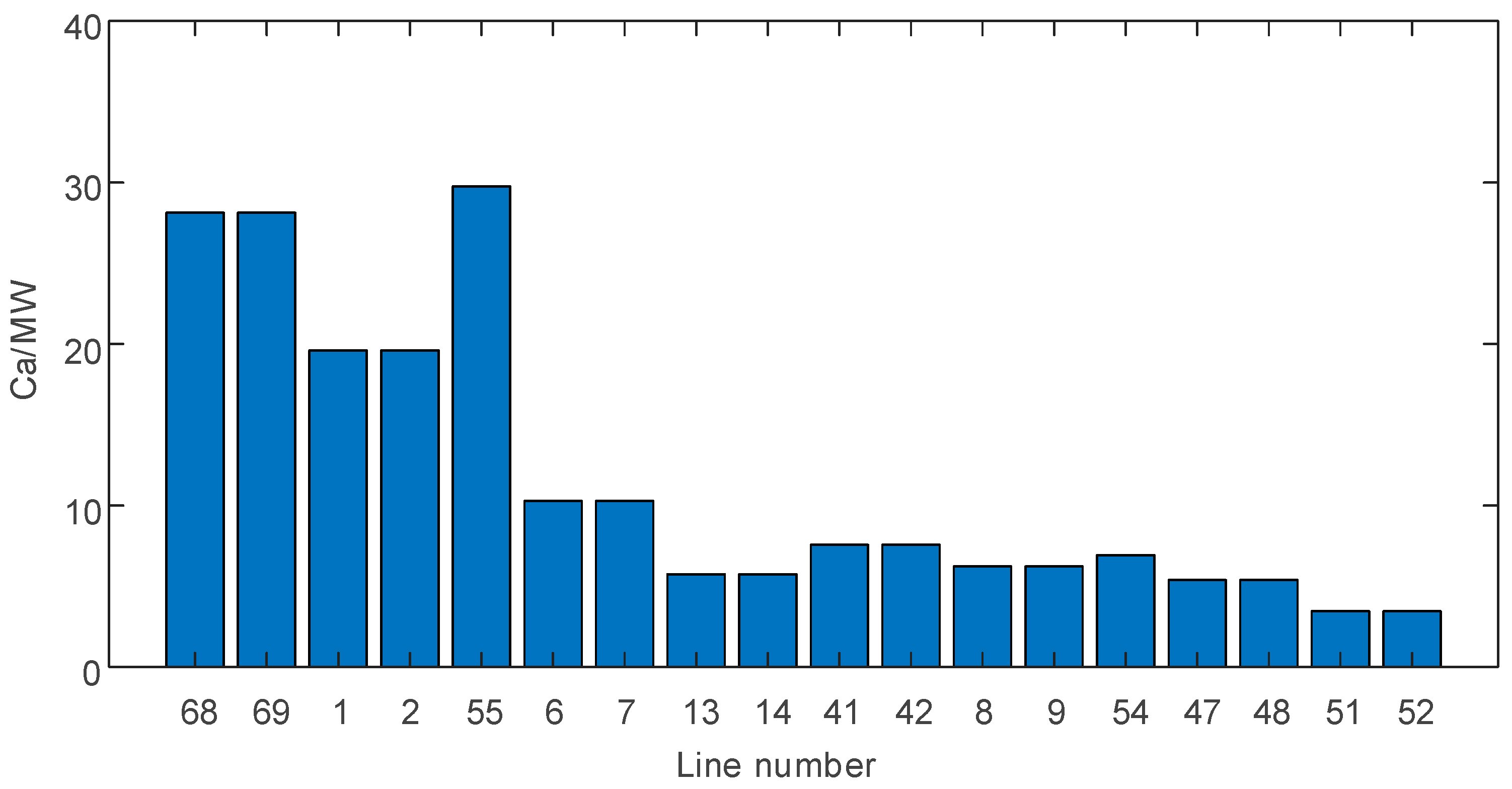
Based on the calculation results of the electrified railway traction load power mentioned earlier, perform power flow analysis on the mountainous power grid and calculate the real-time transmission capacity P_L for each of the 18 weak transmission lines. Then, calculate the expansion capacity Ca for the weak lines in the mountainous power grid based on the difference between P_lim,DTR and P_L. The results are shown in

Table 6. Expansion capacity calculation results for weak transmission lines in the mountainous power grid.

Line Number	Ca/MW	Line Number	Ca/MW
68	28.1331	41	7.5682
69	28.1331	42	7.5682
1	19.6074	8	6.2254
2	19.6074	9	6.2254
55	29.7695	54	6.9386
6	10.2889	47	5.3951
7	10.2889	48	5.3951
13	5.74420	51	3.4623
14	5.74420	52	3.4623

and Figure 7.

Furthermore, to quantitatively analyze the impact of dynamic expansion of transmission lines on the reliability level of the mountainous power grid, consider calculating the reliability indicators of the grid after dynamic expansion of the transmission lines. First, simulate the grid operating conditions using the Monte Carlo method within the context of integrating the electrified railway into the mountainous power grid. Then, based on the calculated expansion capacities of the weak transmission lines, readjust the transmission capacity limits of the lines and update the relevant transmission capacity constraints in the optimal power flow model of the grid.

Analyze the grid operating conditions based on the optimal power flow model, record the load-shedding conditions of the mountainous power grid, and calculate the relevant reliability indicators. The calculation results are shown in

Table 7. Reliability indicator calculation results for the mountainous power grid (after line dynamic expansion).

Indicator Type	Case
LOLP	0.0127
LOLF/(Times·h−1)	0.3421
EDNS/(MW·h−1)	19.3611

.

From the table above, it can be seen that after considering the dynamic expansion of weak transmission lines, the reliability indicators of the mountainous power grid, including LOLP, LOLF, and ENDS, have shown a downward trend. Among these, the decrease in the LOLP indicator is particularly notable. With changes in train operation conditions, the reduction rates of LOLP are 93.89%, 92.59%, and 90.46%, respectively. Compared to before the dynamic expansion of the lines, the reliability level of the grid has significantly improved. Therefore, addressing the issue of decreased reliability of the mountainous power grid caused by fluctuating traction loads, the proposed dynamic expansion of the transmission lines can effectively enhance the reliability of the grid and reduce the impact of traction load fluctuations on the reliability of the power supply in mountainous areas.

4.3.2. Comparison of Reliability Indicator Calculation Results for the Mountainous Power Grid Before and After Standby Capacity Configuration

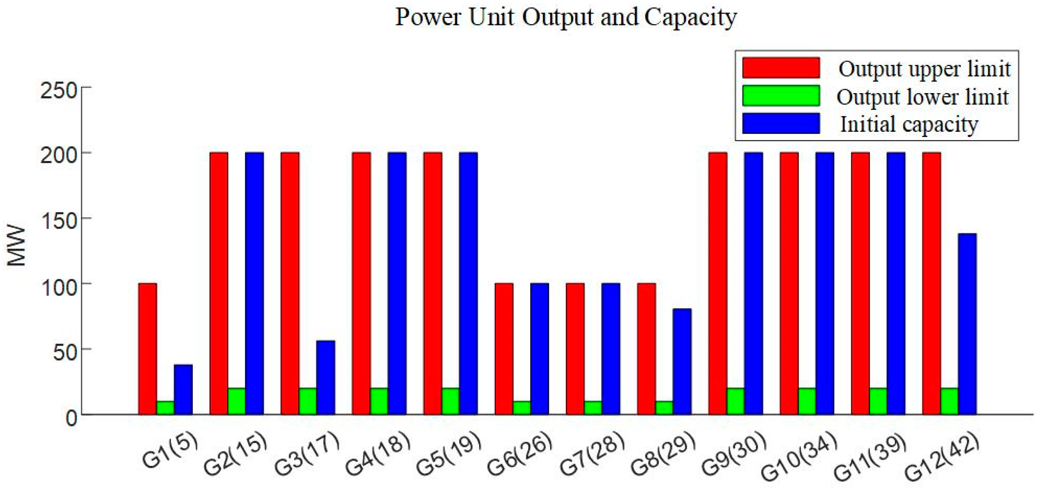
The proposed power grid in the western mountainous region has a total of 12 generating units. The generation output parameters and the locations of the generators are shown in

Table 8. Parameters of each generating unit in the mountainous power grid.

Unit Number and Node Number	Output Upper Limit/MW	Output Lower Limit/MW	Initial Capacity/MW	Ramp Rate/(MW·min−1)
G1 (5)	100	10	38	17
G2 (15)	200	20	200	44
G3 (17)	200	20	56.34	25
G4 (18)	200	20	200	32
G5 (19)	200	20	200	38
G6 (26)	100	10	100	21
G7 (28)	100	10	100	18
G8 (29)	100	10	80.66	11
G9 (30)	200	20	200	62
G10 (34)	200	20	200	59
G11 (39)	200	20	200	48
G12 (42)	200	20	138	77

and Figure 8.

First, based on the calculation results of the electrified railway traction load power mentioned earlier, calculate the reliability contribution γ for each of the 12 generators in the grid. The results are shown in

Table 9. Reliability contribution calculation results for generating units in the mountainous power grid.

Unit Number	Reliability Contribution γ	Unit Number	Reliability Contribution γ
G1 (5)	0.0001	G7 (28)	0.2555
G2 (15)	0.0612	G8 (29)	0.3167
G3 (17)	0.0612	G9 (30)	0.3778
G4 (18)	0.1092	G10 (34)	0.4390
G5 (19)	0.1332	G11 (39)	0.5001
G6 (26)	0.1944	G12 (42)	0.5613

.

From Table 9, it can be seen that the generators with higher reliability contributions, namely G8 to G12, are mainly distributed near node 1, node 32, and node 45, which are connected to traction loads. With the continuous operation of the electrified railway, these nodes where the generators are located are the main force for power flow transmission in the grid. Any insufficiency in generator output at these nodes could pose a serious threat to the reliable operation of the grid.

Based on the reliability contribution results of the grid generators, determine the standby capacity configuration scheme for the mountainous power grid, considering both reliability and economic factors. Under the constraints of the generator standby capacity configuration, sequentially increase the standby capacity of generators G12 to G8 with a fixed simulation step size until the iteration termination condition is met. The simulation step size is ΔR = 1 MW, the unit cost of power outage loss for the grid is α = 6780 CNY/MW, and the unit cost of standby capacity for the grid generators is β = 136 CNY/MW [32]. The standby capacity configuration scheme for the 12 generators in the mountainous power grid is shown in

Table 10. Standby capacity configuration scheme for generators in the mountainous power grid.

Unit Number	Reliability Contribution γ	Unit Number	Reliability Contribution γ
G1	0	G7	19
G2	21	G8	26
G3	21	G9	28
G4	28	G10	31
G5	17	G11	39
G6	16	G12	46

.

From Table 10 and Figure 9, it can be seen that the configuration scheme of the standby capacity for generators in the mountainous power grid is affected by the uncertain factor of shock fluctuating the traction load: as the traction load power increases, the total standby capacity configuration for all units is 292 MW, 364 MW, and 464 MW, respectively. Based on this, in order to further study the impact of the standby capacity configuration on the reliability and economy of the mountainous power grid, the reliability index EDNS and the corresponding total operating cost of the mountainous power grid before and after the standby capacity configuration were calculated, as shown in

Table 11. Comparison of reliability indicators and total operating costs for mountainous power grid.

Train Operating Case	Before Standby Capacity Configuration		After Standby Capacity Configuration
	Cost/CNY	EDNS/(MW·h−1)	Cost/CNY	EDNS/(MW·h−1)
Case	192,332.52	27.9961	110,572.65	10.2547

.

As shown in the Table 11, after considering standby capacity configuration for generating units in the mountainous power grid, both the reliability indicator EDNS and the corresponding total operating Cost significantly decrease. With changes in train operating conditions, the reduction rates of the reliability indicator EDNS are 42.51%, 40.49%, and 30.09%, respectively, while the reduction rates of the total operating Cost are 63.37%, 59.61%, and 50.52%, respectively. This indicates that, after considering the standby capacity configuration for the mountainous power grid, the grid can effectively meet the need for standby capacity to handle random fluctuations and high-power traction loads during operation, reducing the risk of power outages. Additionally, with an appropriate increase in the grid’s standby capacity, the total operating cost of the grid decreases, achieving a comprehensive coordination of grid reliability and economic efficiency.

4.4. Parametric Sensitivity Assessment for Reliability Enhancement Strategies

In the analysis of this section, we have observed significant changes in the power grid reliability indices under different cases. Due to the reduction in train departure intervals and station stop times, the impulsive fluctuations of the traction load have increased, posing a greater challenge to the power supply capacity of the mountainous power grid. The following is a specific comparative analysis:

Additional Cases:

Case 1: Train departure interval of 15 min and stop time at the station of 10 min;

Case 2: Train departure interval of 10 min, station stop time of 10 min;

Case 3: Train departure interval of 10 min, station stop time of 5 min.

4.4.1. Comparative Analysis of Reliability Indices Before and After Dynamic Capacity Expansion of Transmission Lines

LOLP (Loss of Load Probability) changes: As can be seen from

Table 12. Calculation results of reliability indices for mountainous power grids under different cases.

Type of Indicator	Case 1	Case 2	Case 3
LOLP	0.2081	0.3134	0.4998
LOLF/(times·h−1)	1.5224	2.0087	4.1503
EDNS/(MW·h−1)	27.9961	38.0503	45.3472

, with the addition of Case 2 and Case 3, the LOLP increased from 0.2081 in Case 1 to 0.3134 in Case 2, and further rose to 0.4998 in Case 3. This indicates that the probability of load curtailment has significantly increased under the condition of more frequent train operations. The reason lies in the fact that the increased number of trains has led to more intense load fluctuations, heightened the risk of line overloading, and consequently caused a decline in the overall reliability of the power grid.

LOLF (Loss of Load Frequency) changes: The LOLF increases with the shortening of the train departure interval, rising from 1.5224 (Case 1) to 2.0087 (Case 2), and even doubling to 4.1503 in Case 3. This indicates that when trains depart more frequently, the frequency of load curtailment in the power grid significantly increases.

EDNS (Expected Demand Not Served) changes: The average load loss (EDNS) also significantly increased with the change in cases, rising from 27.9961 MW/h in Case 1 to 38.0503 MW/h in Case 2, and reaching the highest value of 45.3472 MW/h in Case 3. This indicates that when the load demand is higher, the mountainous power grid is unable to fully meet the demand, resulting in more severe load loss.

These changes indicate that the mountainous power grid has insufficient carrying capacity and decreased reliability under high load conditions, and optimization plans are needed to improve the power grid stability. This is due to the intensified power fluctuations at the grid nodes, which have increased the frequency of power flow redistribution, thereby increasing the probability of line overloading.

In order to alleviate the reliability decline caused by load fluctuations, we have examined the impact of the dynamic capacity expansion of transmission lines and the optimization of reserve capacity on power grid reliability under different cases, and conducted a comparative analysis of the results.

From

Table 13. Calculation results of reliability indices for mountainous power grids under different cases (after dynamic capacity expansion of transmission lines).

Type of Indicator	Case 1	Case 2	Case 3
LOLP	0.0127	0.0232	0.0475
LOLF/(times·h−1)	0.3421	0.6443	2.1337
EDNS/(MW·h−1)	19.3611	22.6870	30.0064

and

Table 14. Reserve capacity configuration scheme for generators in the mountainous power grid after the addition of new cases.

Unit Number	Reserve Capacity Configuration Value/MW
	Case 1	Case 2	Case 3
G1	0	0	0
G2	21	34	48
G3	21	34	48
G4	28	30	39
G5	17	22	31
G6	16	23	32
G7	19	24	38
G8	26	30	39
G9	28	34	42
G10	31	43	47
G11	39	44	48
G12	46	46	52

, and Figure 10, a detailed analysis of the three reliability indices (LOLP, LOLF, EDNS) before and after the dynamic expansion of the transmission line can be conducted, as shown below:

LOLP changes: After the dynamic capacity expansion of the transmission lines, the LOLP (Loss of Load Probability) has decreased in all cases, but it still increases with the load. Specifically, the LOLP in Case 1 decreased from 0.2081 to 0.0127, in Case 2 it dropped from 0.3134 to 0.0232, and in Case 3 it fell from 0.4998 to 0.0475. This indicates that dynamic capacity expansion has a significant effect on improving reliability, but in Case 3 with a higher load, the reduction is relatively limited, and other supplementary measures are still needed.

LOLF changes: As shown in Table 8, the LOLF (Loss of Load Frequency) also decreased after the dynamic expansion. In Case 1, it dropped from 1.5224 to 0.3421, in Case 2 it fell from 2.0087 to 0.6443, and in Case 3 it decreased from 4.1503 to 1.2789. This shows that line expansion can effectively reduce the frequency of load loss in the power grid, making its operation more stable.

EDNS changes: After the dynamic expansion, the EDNS (Expected Demand Not Served) also decreased. In Case 1, it dropped from 27.9961 MW/h to 19.3611 MW/h, in Case 2 it fell from 38.0503 MW/h to 22.6870 MW/h, and in Case 3 it decreased from 45.3472 MW/h to 30.0064 MW/h. This indicates that dynamic expansion can effectively alleviate load loss, but in Case 3 with a larger load, there is still significant pressure.

It can be seen from the above table that the dynamic expansion scheme has a noticeable effect when the load is relatively low, but additional optimization measures, such as reserve capacity configuration, are still needed in cases with a larger load to further improve the reliability of the power grid.

4.4.2. Comparative Analysis of Reliability Indices Before and After Reserve Capacity Configuration

The prerequisite for this simulation result is that the parameter information of each power generation unit in the mountainous power grid and the calculation results of the reliability contribution of the power generation units in the mountainous power grid are shown in Table 8 and Table 9, respectively. After the addition of Case 2 and Case 3, the reserve capacity configuration scheme for the generators in the mountainous power grid is as follows:

Based on the table above, calculate separately for Case 2 and Case 3: the reliability index EDNS and the corresponding total operating cost for the mountainous power grid before and after reserve capacity configuration. The results are shown in

Table 15. Comparison of the calculated results of reliability indices and total operating cost for the mountainous power grid.

Train Operating Case	Before Reserve Capacity Configuration Before Standby Capacity Configuration		After Standby Capacity Configuration
	Cost/CNY	EDNS/(MW·h−1)	Cost/CNY	EDNS/(MW·h−1)
Case 1	192,332.52	27.9961	110,572.65	10.2547
Case 2	2,614,720.2	38.0503	1,556,051.5	15.3697
Case 3	311,533.89	45.3472	217,888.92	22.4358

.

Based on the data changes in Table 15 and Figure 11, a detailed analysis of the changes in the indicators (EDNS, cost) before and after the configuration of the generator’s backup capacity can be conducted:

Changes in total operating cost: After the optimization of reserve capacity, the total operating cost has significantly decreased in all cases. In Case 2, it dropped from CNY 2,614,720.2 to CNY 1,556,051.5, and in Case 3, it fell from CNY 311,533.89 to CNY 217,888.92. The newly added case data show that changing the train departure intervals and station stop times, which have a high load impact on the mountainous power grid, does not affect the effect of reserve capacity in effectively reducing the power grid operating cost.

Changes in EDNS: After the optimization of reserve capacity, the EDNS has significantly decreased. In Case 2, it was reduced by 59.61%, and in Case 3, it was reduced by 50.52%. This indicates that the optimization of reserve capacity can effectively reduce load loss and still significantly improve the power grid reliability under higher load conditions.

In conclusion, the reserve capacity optimization plan not only effectively reduces the total operating cost of the power grid but also improves the power grid reliability under higher load conditions, indicating that the plan has good adaptability and stability under different load cases.

5. Conclusions

This paper proposes a method for calculating the reliability of mountainous power grids considering the access of electrified railways. Using the example of a 200 km/h passenger and freight electrified railway accessing into a western mountainous power grid, this study established a dynamic model for traction load and assessed the impact of traction load access on the reliability of the mountainous power grid. This study identified weak points in the grid’s reliability and, finally, proposed reliability enhancement schemes for the mountainous power grid. The specific conclusions are as follows:

(1)

Unlike conventional power loads, electrified railway traction loads have characteristics of random fluctuations, high power, and strong impacts due to factors such as track environment, traffic density, and locomotive models. When accessing electrified railways into mountainous power grids, the traction load power continuously changes with the ongoing operation of traction locomotives, causing variations in the injected power at grid nodes. Meanwhile, the power flow in the mountainous grid experiences sudden and severe fluctuations, leading to non-constant reliability parameters for the lines, with the failure outage rate increasing as the line flow increases.

(2)

By comparing the reliability indicators of the mountainous power grid before and after the access of traction loads, it can be seen that as the intervals between locomotive departures and station stops decrease, the reliability indicators of the mountainous power grid increase, leading to a significant decline in reliability. The weak points in the reliability of the mountainous power grid are mainly located near the nodes with traction loads. The impact of the fluctuating traction loads on the power flow in the lines near these nodes is significant, exacerbating the risk of line failures and outages.

(3)

The proposed methods for dynamic expansion of transmission lines and standby capacity configuration in mountainous power grids effectively mitigate the decline in reliability caused by the integration of electrified railways. For the identified vulnerable transmission lines in mountainous power grids, capacity expansion is implemented through rational increases in power transfer capabilities. Reliability evaluations are conducted for both dynamic line capacity upgrades and optimized backup capacity allocation configurations. Comparative analysis of reliability indices before and after implementation demonstrates the effectiveness of the proposed electrified railway-integrated reliability enhancement scheme for mountainous power grids. Additionally, after appropriately configuring standby capacity for the mountainous power grid, not only can the risk of power outages be reduced, but the overall operating cost of the grid can also decrease, achieving a comprehensive coordination of grid reliability and economic efficiency.