3.1. Dataset Description
The dataset employed in this study consists of operational data collected from four compressors at a leather tanning facility located in Santa Croce sull’Arno, Italy. This facility was selected due to its significant energy consumption and the critical role that compressors play in its production processes. The choice of compressors with similar functions and characteristics ensures that our findings are relevant and can be generalized across comparable industrial settings.
Data collection was conducted with an hourly granularity, which is crucial for enabling timely interventions and facilitating a thorough analysis of energy consumption trends throughout the day. This level of detail allows for the identification of patterns that may indicate potential anomalies, thereby enhancing our predictive maintenance capabilities. The specific timeframe for data collection spans from March to June 2024. This period was chosen because it reflects full operational capacity, as the facility tends to operate at reduced levels during the summer months due to employee holidays. Consequently, data from March to June provide a more accurate representation of normal operational conditions, making it ideal for training and testing our models.
The dataset comprises several critical features that are instrumental in assessing compressor performance and detecting anomalies such as current (A), power factor (CosPhi), energy consumption (kWh), reactive energy (VARh), and voltage (V) (see
Table 1).
These features are critical for our anomaly detection framework. For example, monitoring current levels helps identify deviations that may indicate potential electrical issues or inefficiencies in compressor operation. The power factor is particularly important as it reflects how effectively the compressors convert electrical energy into mechanical work; a low power factor could signal underlying problems that require attention. Energy consumption metrics provide insights into operational trends, enabling us to detect anomalies that could lead to costly downtimes or maintenance needs.
In addition to their role in detecting anomalies, these features are integral to our overarching goal of preventing issues before they arise. By closely monitoring current levels, power factor, and energy consumption metrics, we can not only identify existing inefficiencies but also predict potential failures. This proactive approach enables us to implement maintenance strategies that address issues early on, thereby minimizing the risk of costly downtimes and enhancing the overall reliability of compressor operations.
By utilizing this comprehensive dataset, our research aims to develop a robust predictive maintenance framework that enhances the reliability and efficiency of compressors in energy-intensive industrial applications. The integration of these features into our machine learning models will allow for a nuanced understanding of compressor behavior, ultimately contributing to improved operational performance, reduced maintenance costs, optimizing performance and sustainability, and ensuring that compressors operate within their ideal parameters and reducing the likelihood of unexpected breakdowns.
3.1.1. Data Pre-Processing
Data pre-processing is an essential phase in preparing the dataset for effective anomaly detection and predictive maintenance analysis. In this study, we structured our pre-processing efforts into two main phases: the aggregation of individual measurements from each compressor (Section Aggregation of Individual Measurements from Each Compressor) and the correction of anomalous values (Section Correction of Anomalous Values).
Aggregation of Individual Measurements from Each Compressor
The first phase involved began by establishing a comprehensive time frame for data collection, spanning from 17 March 2024 to 24 June 2024. As already said, this period was selected to capture full-capacity operational conditions, as the facility typically experiences reduced activity during the summer months due to employee vacations. By focusing on this time frame, we ensured that the dataset reflects normal operating behavior, which is crucial for training our predictive models.
Each compressor’s data were stored in a dictionary, where each key corresponds to a compressor name and each value contains a list of DataFrames representing individual measurements. This structure allows for efficient access and manipulation of data.
To ensure data integrity, we conducted several checks on the loaded datasets. We examined each measurement for duplicate timestamps and missing values (NaNs). These checks are crucial as duplicates can lead to erroneous conclusions about equipment performance, while missing values can disrupt model training and evaluation. The results of these integrity checks were compiled into DataFrames for easy reference and analysis. No dataset had either duplicates or missing values.
Following the integrity checks, we proceeded with the aggregation of measurements. We modified the names of the measurements to include their respective units for clarity and consistency. To facilitate analysis across all compressors, we generated a comprehensive timestamp index covering every hour within our specified date range. This ensured that all compressors had aligned time series data, making it easier to compare performance metrics across machines.
Finally, we saved the aggregated datasets for each compressor into a dictionary of DataFrames indexed by the machines’ names for further analysis. This structured approach to data pre-processing not only enhances the quality of our dataset but also lays a solid foundation for subsequent modeling efforts aimed at detecting anomalies in compressor operations. By ensuring that our data are clean, consistent, and well organized, we increase the reliability of our predictive maintenance framework and its ability to identify potential issues proactively.
Correction of Anomalous Values
The correction of anomalous values is a critical step in ensuring the reliability and the accuracy of the dataset used for predictive maintenance analysis. In this study, we focused on identifying and addressing outliers in key performance metrics for the compressors, specifically targeting the columns related to energy consumption and reactive energy.
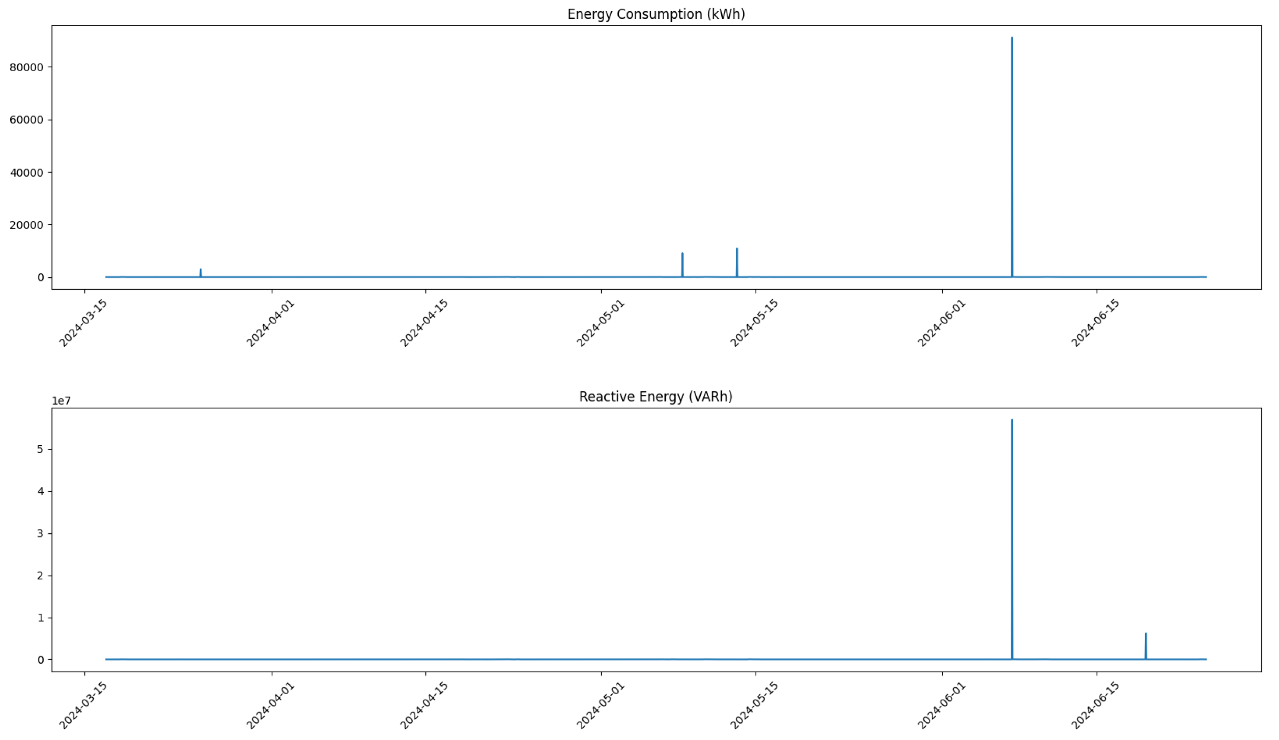
After data aggregation, we visualized the data of each column through plots. This not only provided insight into the overall trends and patterns but also helped the visual identification of potential outliers. Each feature was plotted against time, allowing us to observe fluctuations and irregularities that could indicate anomalous behavior.
For specific columns identified as problematic—namely, Energy Consumption (kWh) and Reactive Energy (VARh)—we established thresholds to define what constituted an anomalous value. For instance, any energy consumption exceeding 200 kWh or reactive energy exceeding 100,000 VARh was flagged as an outlier. This thresholding approach is grounded in domain knowledge regarding expected operational ranges for compressors; values outside these limits are likely indicative of sensor errors or abnormal operating conditions.
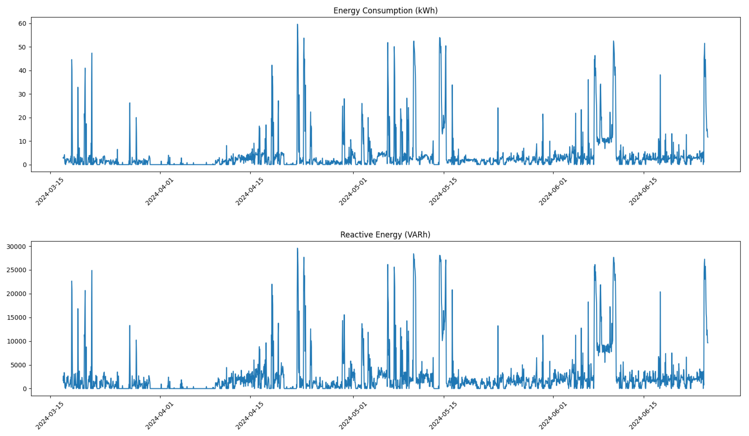
Once outliers were identified, we replaced them with NaN values to be filled using linear interpolation. This process ensures that our dataset remains robust while minimizing the impact of erroneous readings on our predictive models.
Figure 1 and
Figure 2 illustrate these distributions before and after the process of outliers removing.
Finally, after correcting for anomalies and ensuring data integrity, we saved each dataset into a separate Excel file for further use. By implementing these rigorous correction methods and visualizing both pre- and post-correction distributions, we enhance the quality of our dataset, thereby increasing the reliability of our predictive maintenance framework and its ability to detect potential issues within compressor operations effectively.
Thus, as part of the pre-processing phase, we performed a removal of certain outliers corresponding to physically implausible values of reactive energy and energy consumption for the machinery. These outliers were identified based on domain knowledge and statistical analysis. After removing these outliers, we filled in the gaps using linear interpolation, which helped maintain the continuity of the dataset while ensuring that the corrected values remained within a reasonable range.
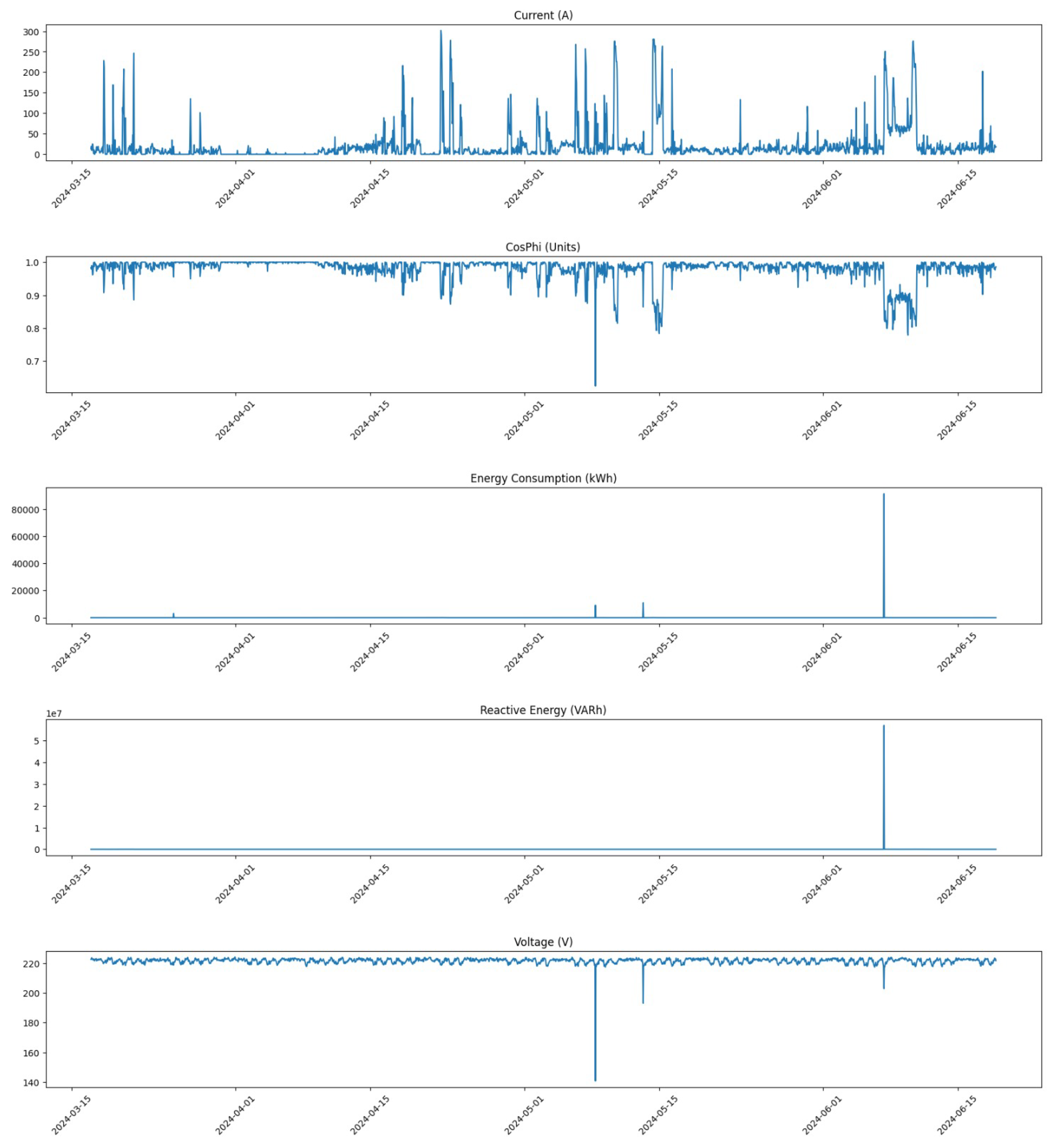
To illustrate the impact of these pre-processing steps, we present several figures showing the distribution of data for Compressor 1 before and after correction.
In
Figure 3, we show the distribution of all feature values for Compressor 1 prior to any corrections. This figure highlights the presence of outliers that may skew analysis and predictions.
Following the correction process,
Figure 4 illustrates the distribution of all feature values for Compressor 1 after corrections were applied. The removal of outliers and the application of linear interpolation result in a more normalized distribution, which is crucial for reliable predictive modeling.
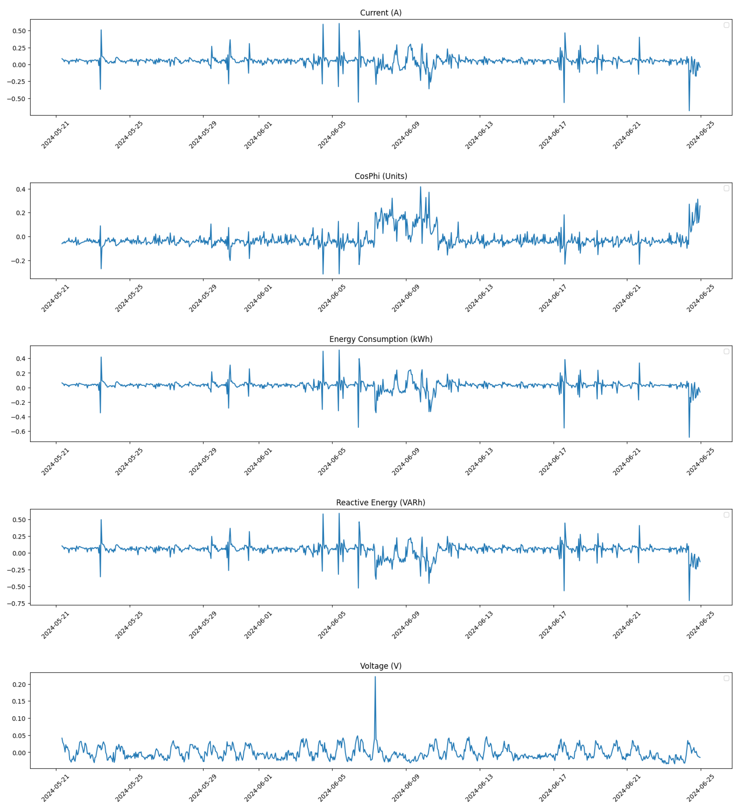
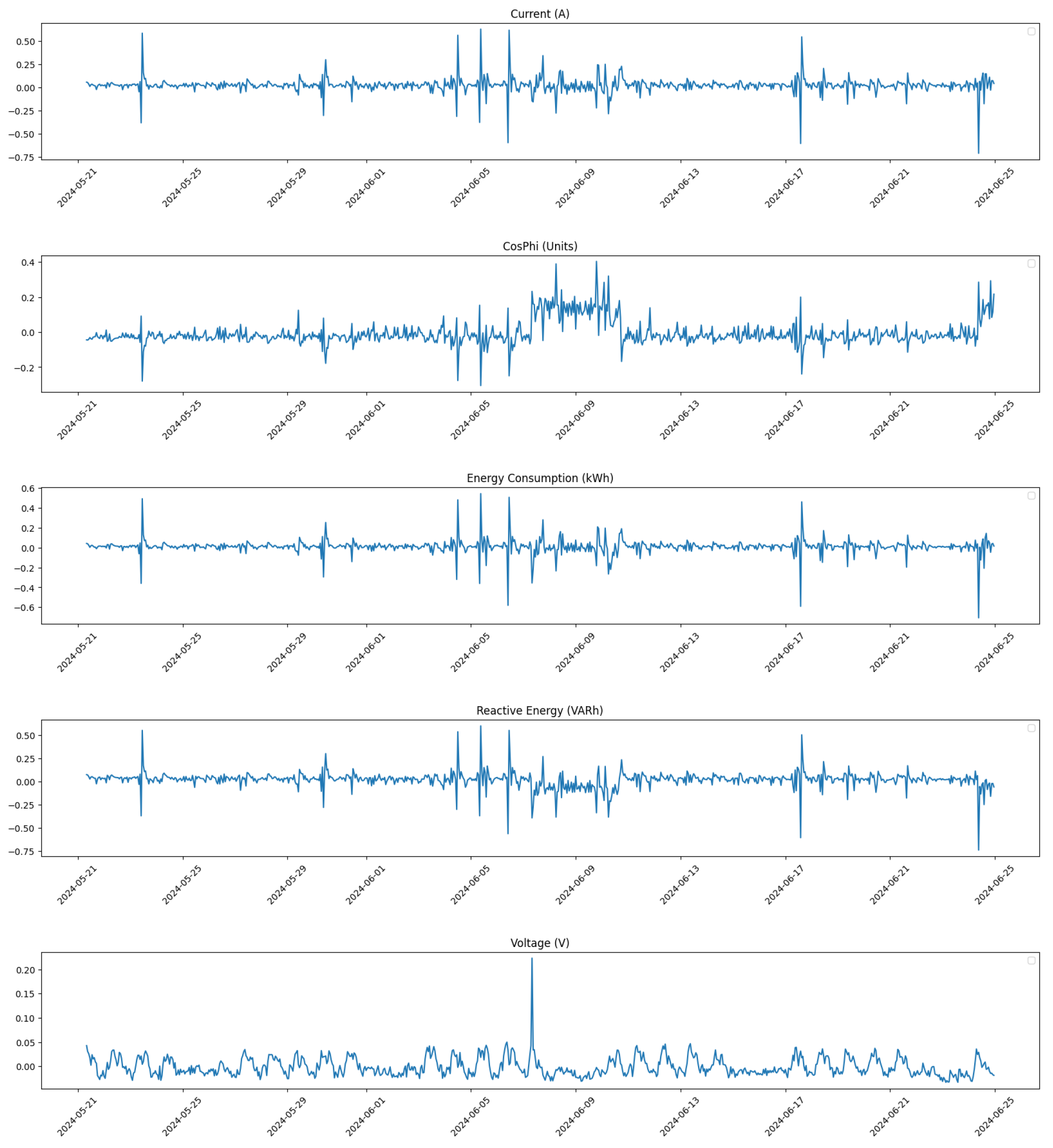
Additionally, we provide a focused analysis on specific time windows to further assess the impact of our corrections.
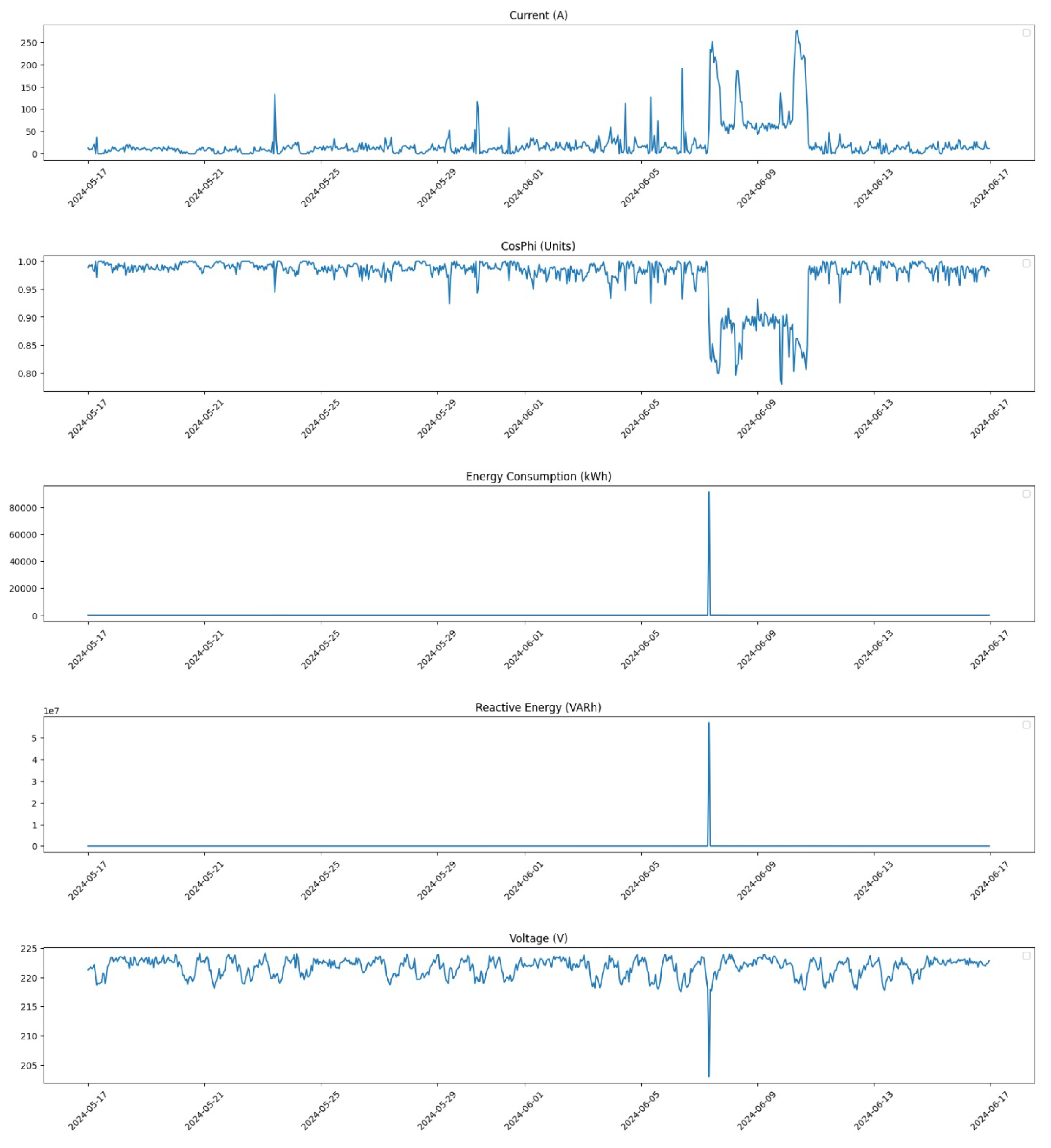
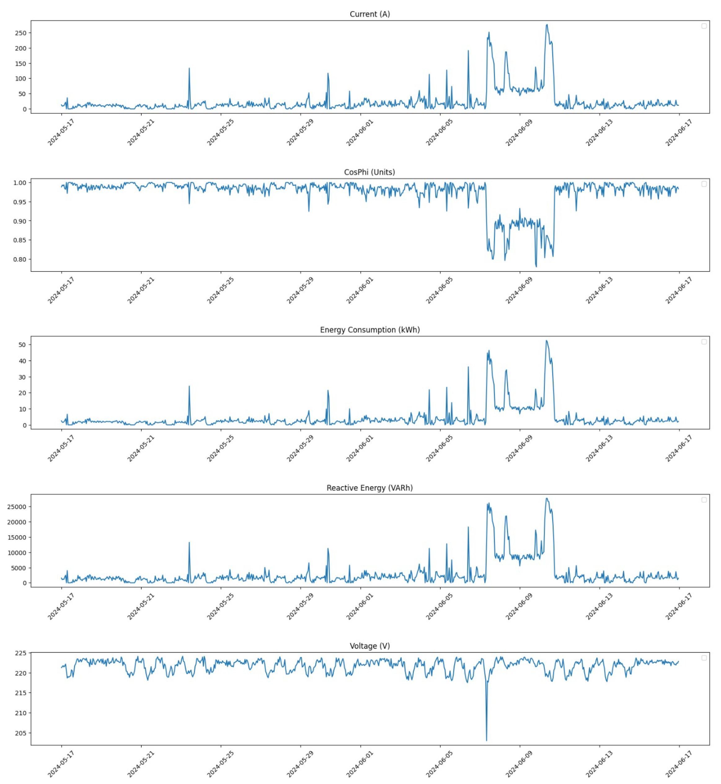
Figure 5 shows the distribution of all feature values within the time window from 17 May 2024 at 00:00 to 16 June 2024 at 23:00 before any corrections were made.
In contrast,
Figure 6 presents the same time window after corrections were applied. The improvement in data distribution is evident, showcasing how our pre-processing steps have enhanced data integrity.
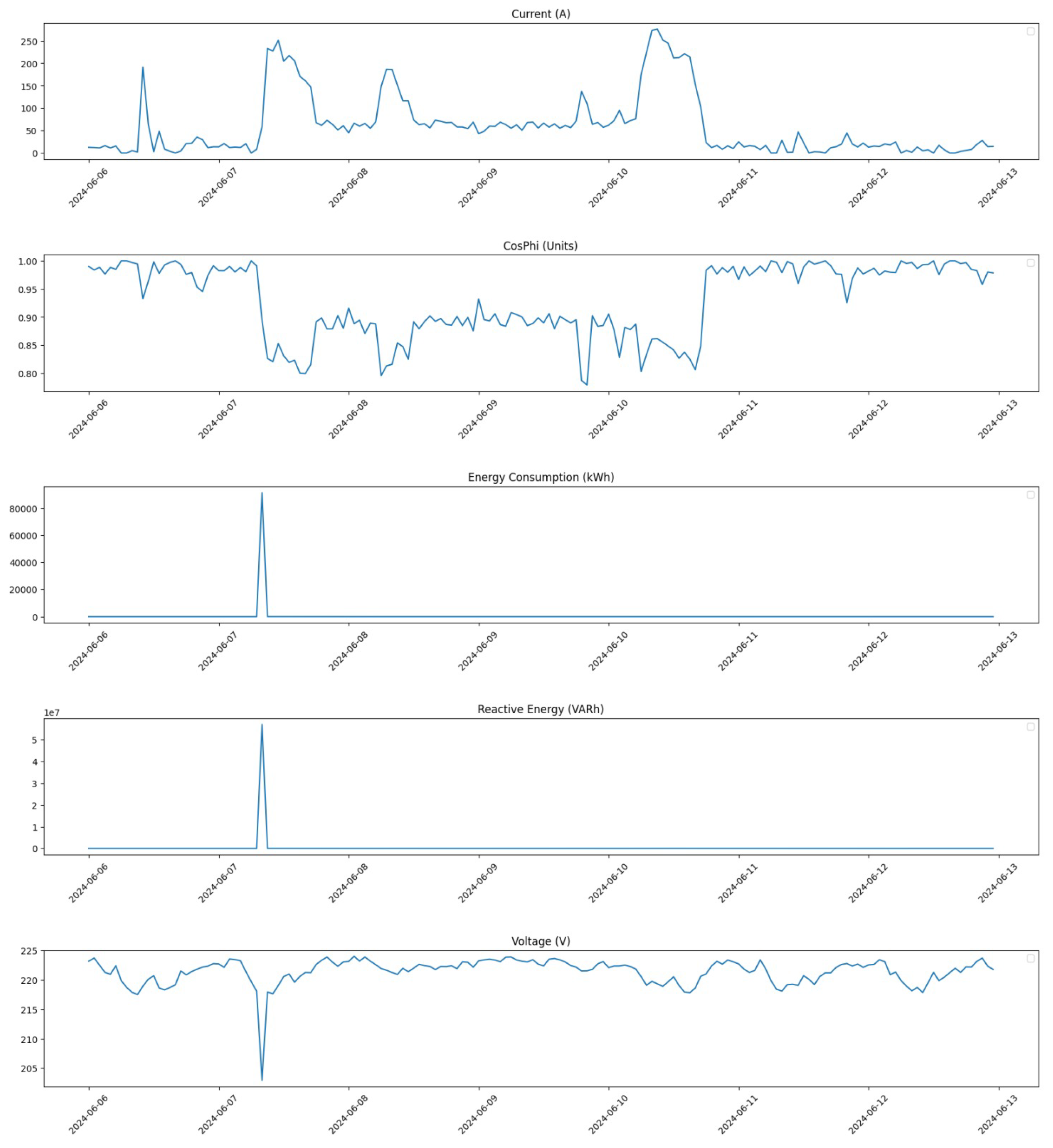
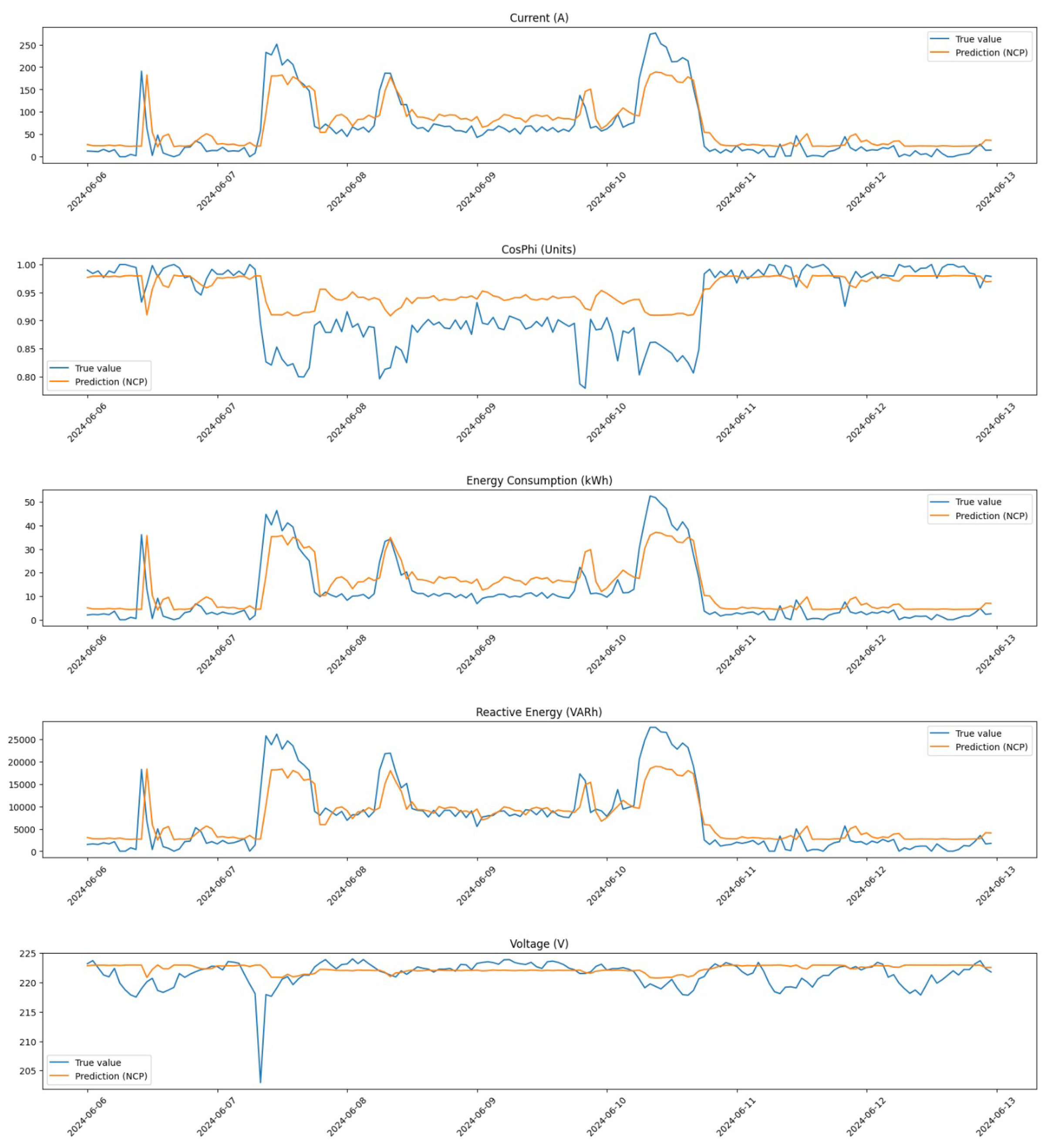
Furthermore, we zoom in on a critical period from 6 June 2024 at 00:00 to 12 June 2024 at 23:00 to analyze changes in detail.
Figure 7 illustrates the distribution during this week before any corrections were implemented.
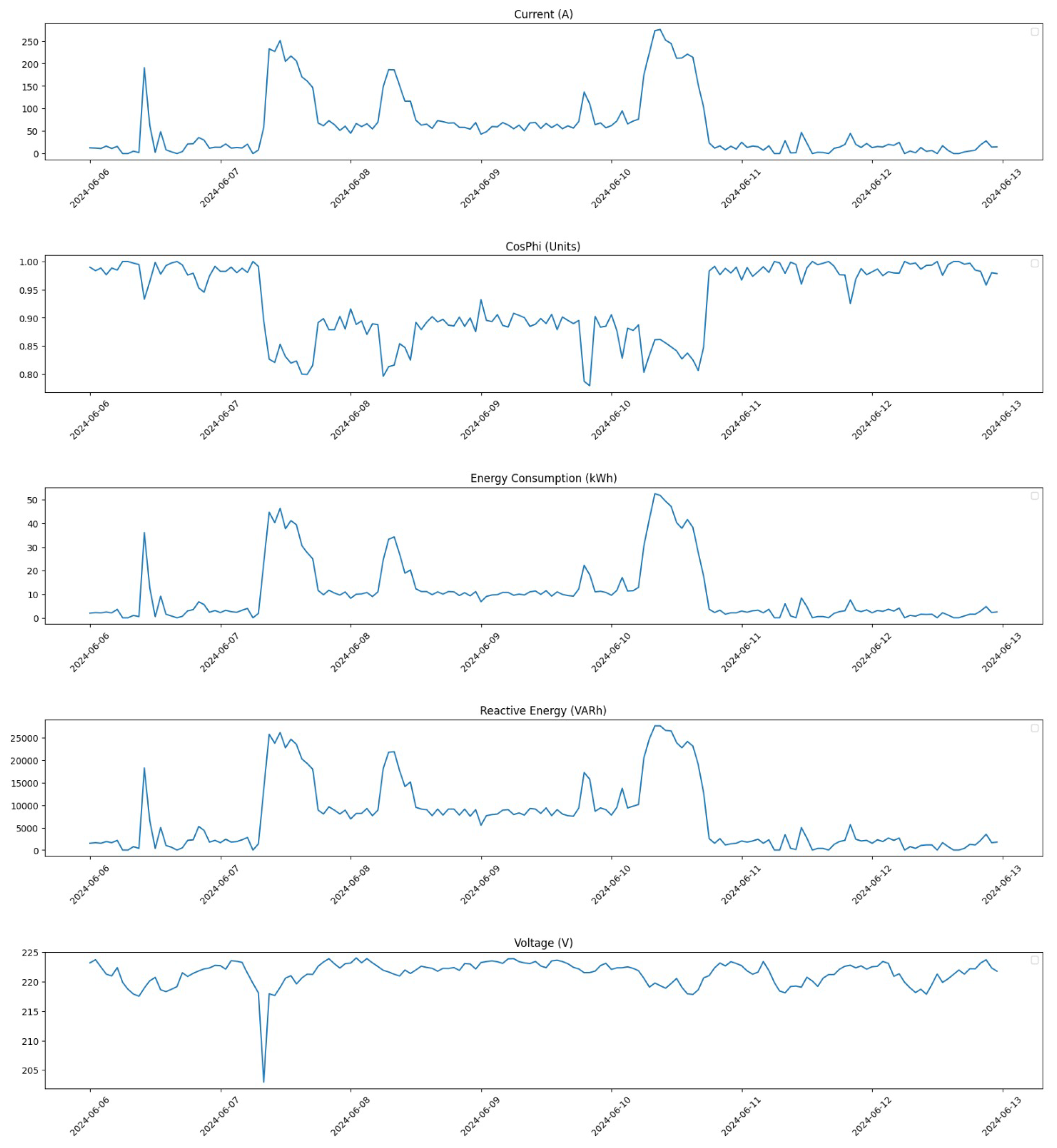
Finally,
Figure 8 shows the distribution for the same period after applying our correction methods. This visualization highlights how effectively our pre-processing has addressed anomalies within this critical time frame.
These figures collectively demonstrate how our pre-processing efforts have significantly improved data quality across different time frames. By addressing outliers and applying linear interpolation where necessary, we have enhanced the dataset’s reliability for subsequent analysis and model training.
3.2. Model Architectures
In this subsection, we present the proposed model architecture designed for anomaly detection in compressors used in leather tanning operations. The primary objective of our architecture is to leverage advanced machine learning techniques, specifically Neural Circuit Policies and Long Short-Term Memory networks, within a federated learning framework. This dual approach aims to enhance the accuracy and interpretability of anomaly detection while addressing critical data privacy concerns inherent in industrial applications.
The architecture is structured to facilitate the integration of local models trained on decentralized data from multiple compressors. By utilizing federated learning, we ensure that sensitive operational data remain on-site, thereby preserving privacy while still benefiting from collaborative learning. The NCPs are particularly noteworthy as they incorporate knowledge of physical constraints through differential equations, allowing for a more nuanced understanding of the system dynamics compared to traditional LSTM models, which primarily rely on historical data patterns.
In the following paragraphs, we will detail the specific components of our model architecture, including the mathematical formulations for both NCPs and LSTMs, as well as the overall design of the federated learning framework. This comprehensive overview will highlight how our proposed architecture effectively combines these methodologies to achieve superior performance in detecting anomalies within compressor operations.
3.2.1. Federated Learning
Federated learning is a decentralized approach to machine learning that enables multiple clients to collaboratively train a shared model while keeping their data localized. This architecture is particularly beneficial in scenarios where data privacy is paramount, such as in industrial applications involving sensitive operational data from compressors in leather tanning facilities. The primary objective of employing FL in our system is to enhance predictive maintenance capabilities without compromising the confidentiality of the data.
In a typical FL setup, there exists a central server that coordinates the training process, while each client holds its own local dataset. Clients independently train their models on local data and subsequently share only the model parameters—rather than the raw data—with the server [
24]. This method significantly mitigates privacy concerns, as sensitive information remains on the client side and is never transmitted over the network. By exchanging model updates instead of raw data, FL aligns with stringent data protection regulations, such as GDPR, making it an ideal choice for industries handling sensitive information.
From an architectural perspective, our FL framework consists of a server and multiple clients, each representing different compressors. The server orchestrates the training process by aggregating model updates from all participating clients. This aggregation can be performed using various strategies, such as averaging the parameters or employing more sophisticated techniques that account for the quality and relevance of each client’s contribution.
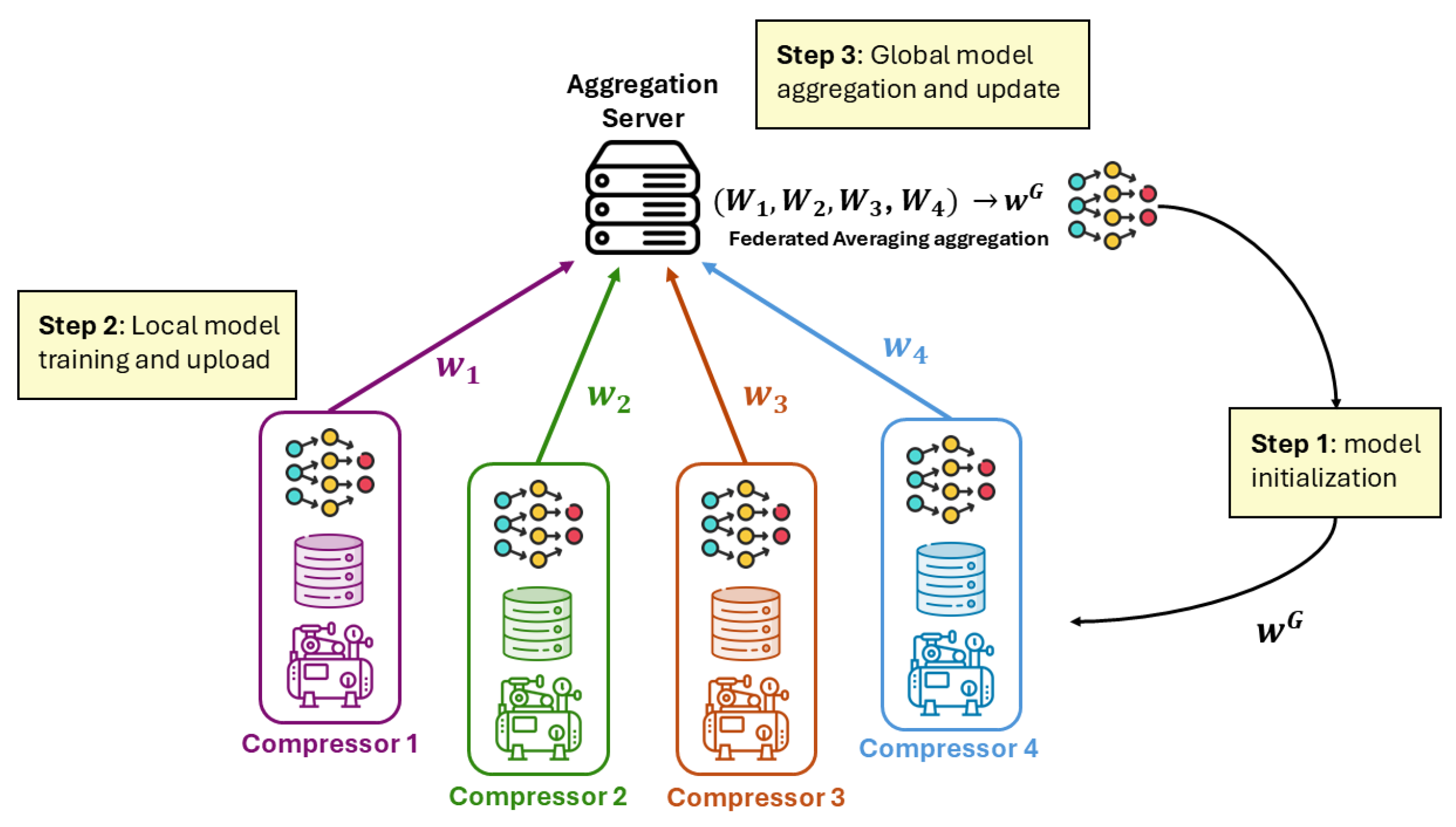
To provide a clearer understanding of the system architecture, we present a general block diagram that illustrates the connections between the different endpoints within our federated learning framework. This diagram visually represents how the server interacts with each client, highlighting the flow of information and the collaborative nature of the training process.
As shown in
Figure 9, the federated learning process begins with clients downloading the current global model from the server at the start of each training round. Each client then independently trains this model using its own local dataset, allowing for personalized adaptation to specific operational conditions without compromising data privacy. Once training is complete, clients send only their computed weights back to the server, ensuring that sensitive local data remains secure and are not shared. The pseudo-code of the training process is shown in Algorithm 1.
| Algorithm 1: Training process of FL |
Input: model architecture , number of rounds R, datasets
Output: trained weights of the global server’s model
- 1:
Initialize the weights of the global server’s model - 2:
Uniquely assign a client to each dataset , - 3:
for
do - 4:
Broadcast with weights to all clients - 5:
for do - 6:
Compute local weights by updating using - 7:
Send to the global server - 8:
end for - 9:
Update global weights: - 10:
end for
|
The server plays a crucial role in aggregating these received weights to update the global model, which is then redistributed to all clients at the beginning of the next round. This iterative process not only enhances model accuracy through collaborative learning but also preserves data privacy—a significant advantage in industrial settings where sensitive operational data may be involved.
In more details, our architecture consists of a central server and multiple clients, each representing a different compressor. The server is responsible for coordinating the training process, while each client independently trains a local model on its dataset. In our implementation, we utilized the Flower framework, which simplifies the setup of FL systems.
The server is initiated by running a script that starts the ‘server.py’ process. This server listens for incoming connections from clients and manages the aggregation of model parameters. Each client is represented by a separate process running ‘client.py’, which connects to the server and participates in the training process.
Each client loads its specific dataset corresponding to one of the compressors (e.g., “Compressor 1”, “Compressor 2”, etc.). The datasets are pre-processed locally to ensure they are ready for model training. This includes handling missing values and normalizing the data with the MinMax method. The clients then train their local models using TensorFlow (version 2.14.1), which allows them to learn from their unique datasets without sharing raw data with the server.
Mathematically, FL can be formalized as follows: let
represent the dataset held by client
k, and let
denote the global model parameters. Each client
k computes an update based on its local dataset:
where
is the local loss function computed on
,
is the learning rate, and
represents the gradient of the loss function with respect to the model parameters. After local training, each client sends its updated parameters
back to the server, which aggregates these updates to form a new global model [
25]:
where
K is the total number of participating clients. This iterative process continues until convergence is achieved or a fixed number of rounds is reached.
The benefits of this federated architecture extend beyond privacy preservation; it also allows for efficient use of computational resources. Clients can train models tailored to their specific operational conditions without needing to centralize vast amounts of data. This decentralized approach not only enhances model robustness by incorporating diverse data distributions but also reduces network bandwidth usage since only model parameters are communicated.
Thus, FL provides a powerful framework for developing predictive maintenance solutions that prioritize data privacy while leveraging collaborative learning across multiple compressors. By integrating this architecture into our anomaly detection system, we aim to improve operational efficiency and reliability in energy-intensive industrial applications.
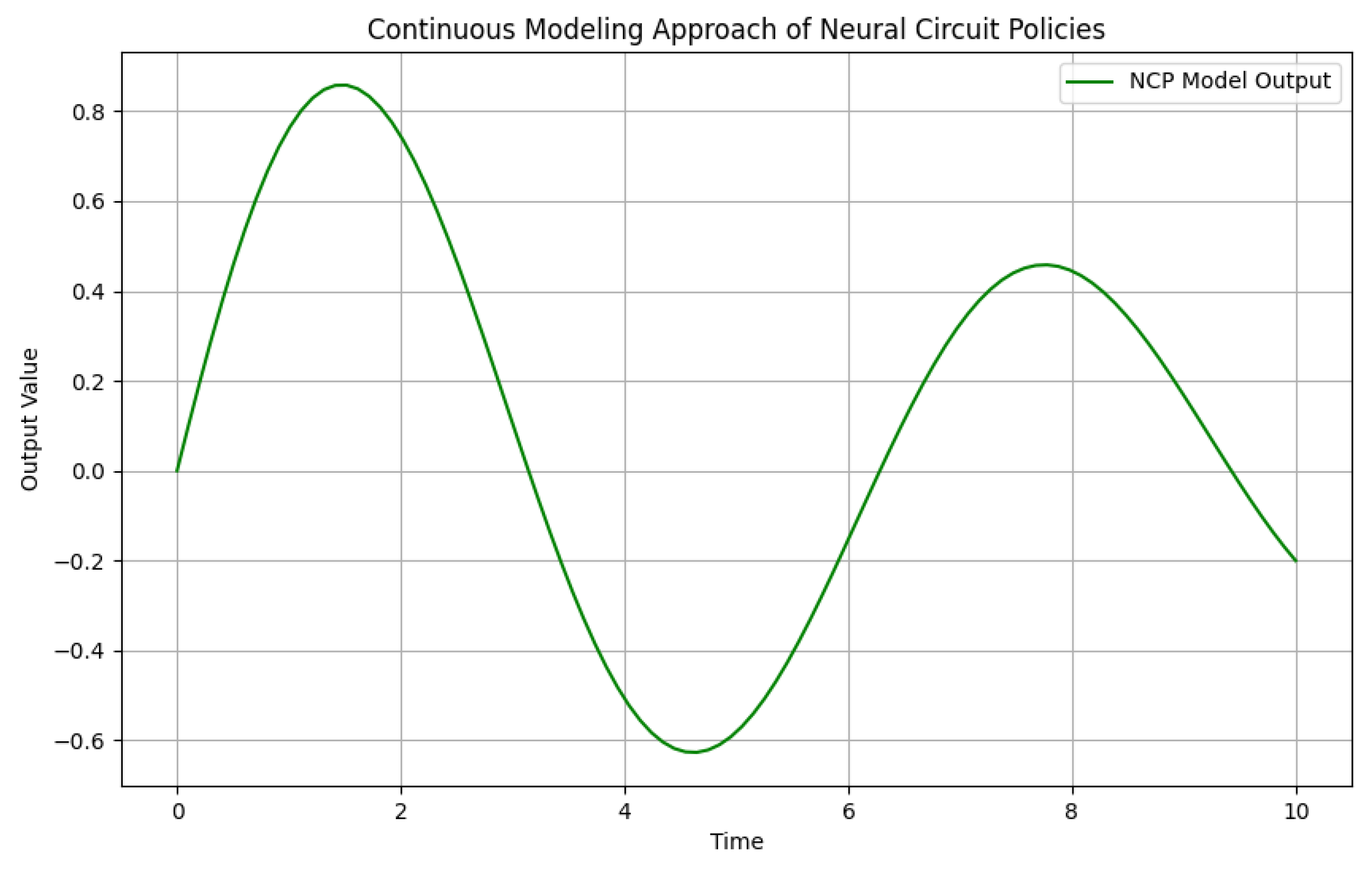
3.2.2. Neural Circuit Policies
Neural Circuit Policies, first proposed by Hasani et al. in [
14], are a novel architecture designed to enhance anomaly detection in time series data, particularly in the context of predictive maintenance for compressors. Indeed, NCPs are structured to mimic biological neural circuits, allowing them to process information through interconnected nodes that represent different features of the input data. Each node in the NCP architecture is designed to capture specific aspects of the time series, enabling the model to learn intricate relationships between variables over time. This architecture is particularly advantageous for anomaly detection, as it facilitates the identification of deviations from expected patterns by analyzing how these nodes interact with each other.
Our implementation of NCPs leverages their ability to model complex temporal dependencies while incorporating knowledge of physical constraints, which is critical for accurately identifying anomalies in operational data.
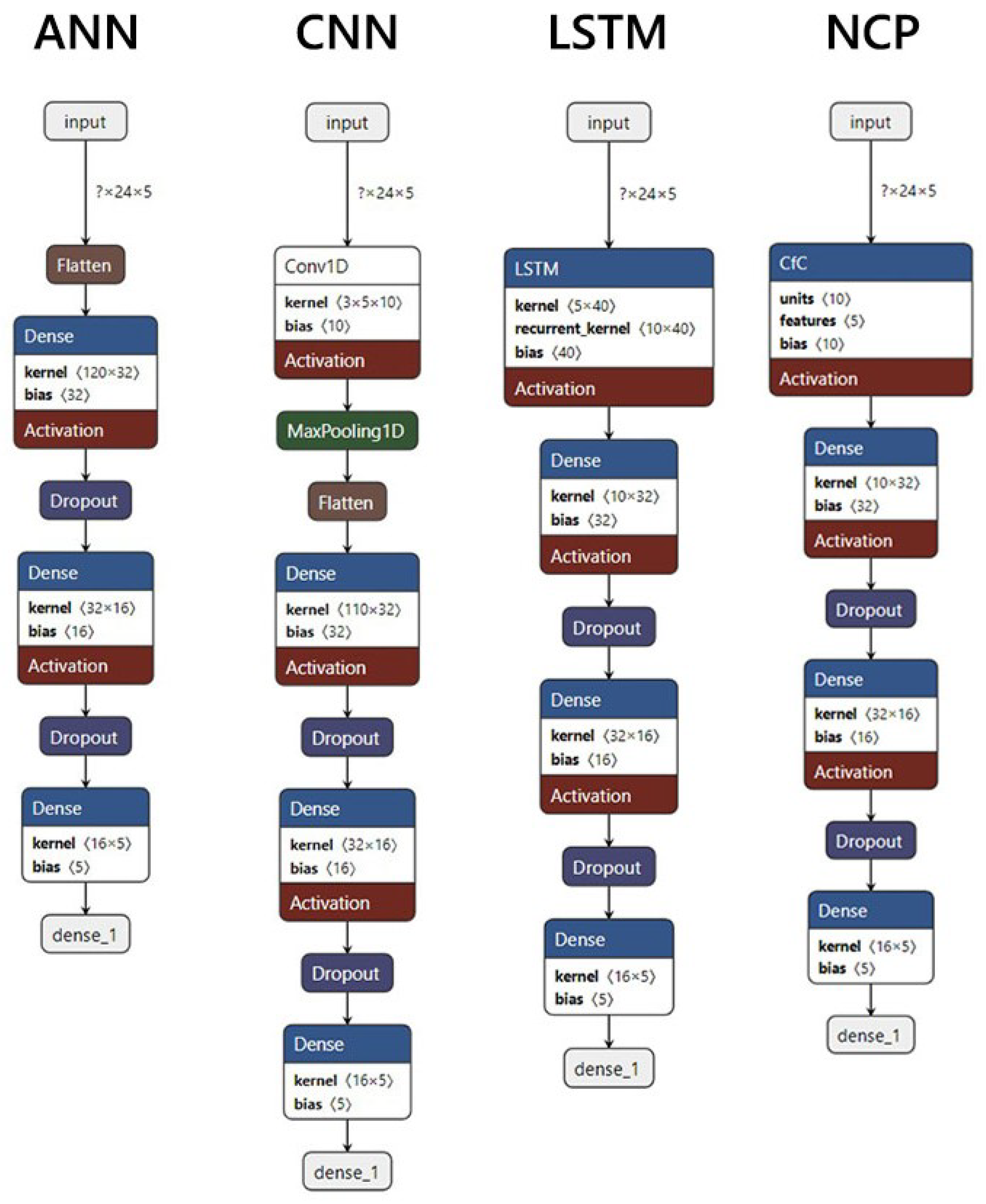
The architecture of our NCP model (see
Figure 10) is structured to effectively process sequences of operational data from compressors. The model is defined using TensorFlow and consists of several key components:
Input Layer: The model begins with an input layer that accepts data shaped as sequences with a specified number of time steps (in our case, 24) and features (5). This structure allows the model to analyze the historical context of compressor operations over time.
NCP Layer (CfC): Central to our architecture is a closed-form continuous-time neural network (CfC) [
26], a pivotal component of the NCP framework. The layer leverages feedback mechanisms to maintain a dynamic representation of the system’s state over time. This approach enables the model to effectively capture temporal dependencies and system dynamics, offering advantages over conventional recurrent architectures like LSTM networks, which primarily operate on discrete time intervals without adequately modeling continuous changes. The input–output expression of the CfC layer is an approximation of the closed-form solution of the Liquid Time Constant (LTC) system
where at a time step
t,
represents the state of a LTC with
d cells,
is an exogenous input to the system with
m features,
is a time-constant parameter vector,
is a bias vector,
f is a neural network parametrized by
, and ⊙ is the Hadamard product.
Dense Layers: Following the CfC layer, we include some fully connected (dense) layers. The first dense layer has 32 units with a ReLU activation function, which introduces non-linearity into the model. This is followed by a dropout layer with a rate of 0.2 which prevents overfitting by randomly setting a fraction of input units to zero during training. Subsequent dense layers further refine the model’s output, ultimately producing predictions that correspond to the original feature set.
Output Layer: The final output layer consists of 5 units with a linear activation function, corresponding to our input features (current, power factor, energy consumption, reactive energy, and voltage). This configuration allows the model to predict these features directly based on learned patterns from historical data.
The mathematical foundation of NCPs provides several advantages for anomaly detection:
Continuous Dynamics: By employing differential equations within the LTC layer, NCPs can capture continuous changes in system states over time. This contrasts with traditional methods that discretize the time domain and may overlook important transitions between states.
Robustness to Noise: The interconnected nature of nodes within the NCP architecture enhances its robustness against noise and outliers in operational data. This is particularly important in industrial settings where sensor inaccuracies can lead to erroneous readings.
Interactivity Among Nodes: Each node in the NCP interacts dynamically with others, allowing for adaptive learning as new data streams are introduced. This interactivity helps in recognizing patterns that may indicate anomalies based on contextual information derived from multiple features.
Our NCP model is configured to handle multiple training channels simultaneously, enabling it to process data from different compressors concurrently. Each channel corresponds to a specific compressor’s dataset, allowing tailored learning while still contributing to a unified global model. This multi-channel capability ensures that the model can learn from diverse operational conditions across various machines, enhancing its generalization ability when detecting anomalies.
Thus, our implementation of Neural Circuit Policies provides a powerful framework for detecting anomalies in time series data through its innovative architecture and mathematical foundations. By integrating physical knowledge with advanced modeling techniques, NCPs enhance our ability to identify operational irregularities in compressors effectively. This makes them particularly suitable for predictive maintenance applications where timely detection of anomalies can lead to significant cost savings and improved operational efficiency.
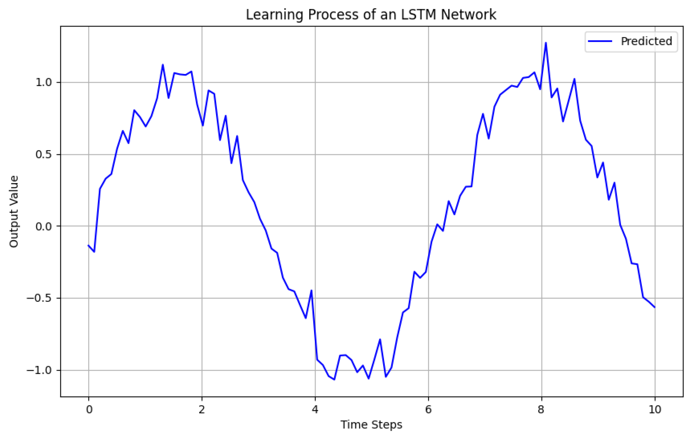
3.2.3. Long Short-Term Memory Networks
Long Short-Term Memory networks are a type of recurrent neural network (RNN) specifically designed to model sequential data and capture long-term dependencies. In our study, we implemented an LSTM architecture to detect anomalies in time-series data from compressors, providing a robust alternative to NCPs. The primary goal of using LSTMs is to leverage their ability to learn from historical sequences, making them suitable for applications where temporal patterns are critical.
The architecture of our LSTM model (see
Figure 10) is structured using TensorFlow and consists of several key components:
Input Layer: The model begins with an input layer that accepts sequences shaped as ‘(timesteps, features)’, where ‘timesteps’ corresponds to the number of past observations (in our case, 24 h), and ‘features’ represents the different operational metrics being monitored (5 features in total).
LSTM Layer: the core of our architecture is a LSTM layer with 10 units and set to ‘return_sequences = False’, meaning it outputs only the final output for the entire sequence. This configuration allows the model to distill information from all time steps into a single representation that can be used for final predictions.
Dense and Dropout Layers: the layers after the LSTM are the same in the proposed NCP architecture.
Output Layer: as in our NCP model, the final output layer consists of 5 units with a linear activation function, corresponding to our input features (current, power factor, energy consumption, reactive energy, and voltage). This structure enables the model to predict these features based on learned patterns from historical data.
The mathematical foundation of LSTMs [
27] provides several advantages for anomaly detection:
Memory cells: LSTMs utilize memory cells that maintain information over long periods, which is crucial for learning dependencies in sequential data. Each memory cell contains three gates: input, forget, and output gates that control the flow of information. The equations governing these gates can be expressed as follows:
Here, are weight matrices, are bias vectors, is the cell state at time t, and is the hidden state output.
Long-term dependencies: By effectively managing long-term dependencies through its gating mechanisms, LSTMs can learn complex temporal patterns that are crucial for detecting anomalies in compressor operations.
Robustness: LSTMs are inherently robust against issues such as vanishing gradients that often plague traditional RNNs. This robustness makes them particularly suitable for processing long sequences of operational data.
Similar to our NCP implementation, our LSTM model is designed to handle multiple training channels simultaneously. Each channel corresponds to a specific compressor’s dataset, enabling tailored learning while still contributing to a unified global model. This multi-channel capability allows the LSTM to learn from diverse operational conditions across various machines, enhancing its ability to generalize when detecting anomalies.
Thus, LSTM networks provide a powerful framework for detecting anomalies in time series data through their specialized architecture and mathematical foundations. By leveraging their ability to learn from historical sequences and manage long-term dependencies effectively, LSTMs enhance our capacity to identify operational irregularities in compressors. This makes them particularly suitable for predictive maintenance applications where timely detection of anomalies can lead to significant cost savings and improved operational efficiency.
3.4. Mathematical Justification for Model Selection
In our approach to anomaly detection for compressors in the leather tanning industry, we focused on comparing LSTM networks and NCPs within a federated learning framework. While various models exist in the literature for anomaly detection, such as Isolation Forest [
28], Local Outlier Factor (LOF) [
29], and Histogram-Based Outlier Score (HBOS) [
30], we intentionally excluded these methods from our comparative analysis. This decision was based on several key considerations that highlight the unique requirements of our application.
To effectively analyze and model anomaly detection in compressors, it is essential to understand the unique characteristics of time-series data generated by these systems, which exhibit temporal dependencies and dynamic behaviors that significantly influence their operational performance.
Compressors generate time-series data characterized by temporal dependencies, which can be mathematically represented as follows:
where
is the observation at time
t,
f is a function capturing the relationship between current and past observations, and
represents noise in the system.
While LSTMs and NCPs are specifically designed to capture the temporal dependencies and continuous dynamics inherent in time-series data, traditional anomaly detection models such as Isolation Forest, LOF, and HBOS lack the necessary mechanisms to effectively analyze such data.
Isolation Forest operates by constructing random decision trees to isolate observations. The underlying assumption is that anomalies are easier to isolate than normal points. However, this method does not take into account the sequential nature of time-series data. Each observation’s context—i.e., its relationship with previous observations—is ignored, leading to potential misclassification of anomalies that may appear normal when considered in isolation but are anomalous in the context of their temporal sequence.
In particular, Isolation Forest isolates anomalies based on random partitions of data points but does not account for their temporal context:
where
is the anomaly score for observation
x,
is the expected path length to isolate point
x, and
is a normalization factor based on the number of observations.
Similarly, LOF measures the local density deviation of a given data point with respect to its neighbors. While it is effective for identifying outliers in static datasets, it fails to account for temporal correlations between observations. In time-series data, the significance of an observation can change dramatically based on its position in the sequence; thus, LOF’s reliance on local density alone is insufficient for capturing these dynamic relationships.
On the other hand, HBOS computes outlier scores based on the distribution of feature values within histograms. This approach is inherently static and does not consider the ordering of observations over time. As a result, HBOS may overlook critical patterns and trends that emerge from the temporal arrangement of data points, leading to inaccurate anomaly detection in scenarios where timing is crucial.
Thus, while Isolation Forest, LOF, and HBOS can be effective in certain contexts, their inability to model temporal dependencies makes them unsuitable for analyzing time-series data generated by compressors. In contrast, LSTMs and NCPs provide robust frameworks capable of capturing these essential dynamics, thereby enhancing the accuracy and reliability of anomaly detection in predictive maintenance applications.
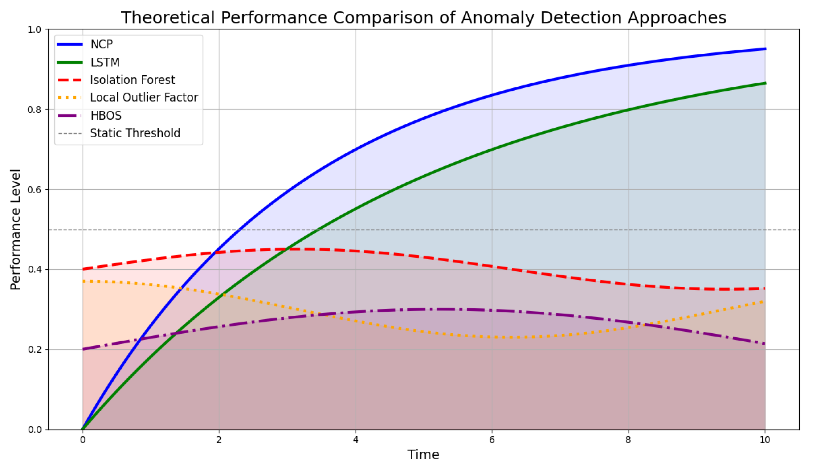
To effectively illustrate the theoretical differences in how various models approach anomaly detection in time-series data generated by compressors, we present a refined conceptual graph (see
Figure 13). This graph simulates the performance characteristics of Long Short-Term Memory networks and Neural Circuit Policies compared to traditional anomaly detection methods such as Isolation Forest, Local Outlier Factor, and Histogram-Based Outlier Score (HBOS).
The curves represent the ability of each model to capture temporal dependencies over time. The LSTM curve demonstrates a gradual improvement in performance as it learns from sequential data, effectively adapting to changes and capturing patterns. This reflects the reality of time-series data where anomalies often evolve gradually rather than appearing abruptly. Similarly, the NCP curve reflects its strength in modeling continuous dynamics through differential equations, showcasing its capability to understand underlying physical processes. By leveraging mathematical representations of system behavior, NCPs can better anticipate shifts in operational conditions.
In contrast, the curves for traditional models indicate a relatively static performance that does not improve significantly over time due to their reliance on isolated observations without considering temporal context. The Isolation Forest curve exhibits minor fluctuations, highlighting its focus on identifying anomalies based solely on their distance from other points, rather than on any temporal progression. The Local Outlier Factor curve shows similar behavior, with slight variations reflecting local density changes but lacking a robust response to temporal trends. This limitation underscores its inability to track evolving patterns in data effectively. The HBOS curve follows a comparable trajectory, emphasizing its reliance on histogram-based scoring that fails to account for sequential dependencies. As a result, these traditional models may miss critical insights that arise from the temporal nature of the data.
This visualization emphasizes why LSTMs and NCPs are more suitable for analyzing time-series data in predictive maintenance applications. Their ability to learn from historical sequences allows for more accurate anomaly detection and ultimately leads to better decision-making in dynamic environments.
3.5. Comparison with Additional Machine Learning Models
To further substantiate our findings and provide a comprehensive evaluation of our proposed approach, we expanded our analysis to include comparisons with additional machine learning models, specifically Convolutional Neural Networks (CNNs) and Artificial Neural Networks (ANNs). This decision was motivated by the need to benchmark our Neural Circuit Policies against a broader spectrum of established models in the context of anomaly detection for compressors used in leather tanning facilities.
The inclusion of CNNs and ANNs in our comparative analysis is particularly relevant given their widespread application in various domains, including time series analysis and anomaly detection. CNNs, known for their ability to automatically extract spatial hierarchies of features through convolutional layers, can be effective in identifying patterns within time series data. On the other hand, ANNs provide a flexible architecture that can model complex relationships within data, making them suitable for capturing non-linear dependencies.
In our comparative analysis, we utilized a consistent set of experimental parameters across all models to ensure a fair evaluation of their performance in anomaly detection for compressors. The hyperparameters for our experiments included a batch size of 8, a learning rate of 0.005, 4 clients participating in the federated learning process, 50 epochs for training, and 5 rounds of training. Each input sequence consisted of 24 timesteps with 5 features, and we allocated 65% of the data for training purposes.
The architecture of the ANN was specifically designed to effectively capture the underlying patterns in the time series data. The model consists of an input layer that accepts sequences shaped according to the defined timesteps (24) and features (5). Following this, we implemented three dense layers with ReLU activation functions. The first two dense layers contain 32 neurons each, allowing the model to learn complex representations of the data. Each of these layers is followed by a dropout layer with a rate of 0.2 to mitigate overfitting by randomly deactivating a fraction of neurons during training. The final output layer consists of 5 neurons with a linear activation function, producing predictions for each feature. The flowchart outlining the structure and operation of the ANN is presented in
Figure 10.
For the CNN, we adopted an architecture that leverages convolutional layers to automatically extract relevant features from the time series data. The model begins with an input layer that accepts sequences shaped according to the defined time steps (24) and features (5). This is followed by a 1D convolutional layer with 10 filters and a kernel size of 3, designed to capture local patterns in the data. After this convolutional layer, we include a max pooling layer with a pool size of 2 to reduce dimensionality while retaining essential features.
The flattened output from the pooling layer is then passed through two dense layers with ReLU activations containing 32 and 16 neurons. Each dense layer is followed by a dropout layer with a rate of 0.2 to enhance generalization. The final output layer consists of 5 neurons with a linear activation function, providing predictions for each feature.
The CNN architecture was chosen due to its proven effectiveness in capturing spatial hierarchies and local dependencies within sequential data, making it particularly suitable for time series analysis. By employing convolutional operations, we aimed to improve the model’s ability to identify patterns indicative of anomalies in compressor operations. The flowchart outlining the structure and operation of the ANN is presented in
Figure 10.
We now present the results of our comparative analysis of the performance of NCPs, LSTM networks, CNNs, and ANNs in detecting anomalies in compressor operations. To evaluate the effectiveness of each model, we employed several performance metrics: Mean Squared Error (MSE), Mean Absolute Error (MAE), Root Mean Squared Error (RMSE), and the Coefficient of Determination (R2). These metrics have been chosen for their ability to provide a comprehensive understanding of model accuracy and predictive capability.
Each metric was chosen for its relevance to our specific problem:
Mean Squared Error (MSE): This metric quantifies the average squared differences between predicted and actual values. MSE is particularly useful in our context because it penalizes larger errors more heavily, which is critical in anomaly detection where significant deviations from expected operational metrics can indicate serious issues. By focusing on squared differences, MSE provides insights into the model’s overall accuracy and helps identify models that perform well across the entire range of data.
Mean Absolute Error (MAE): MAE measures the average absolute errors, offering a more interpretable metric that reflects the average magnitude of errors in predictions without considering their direction. In our application, MAE is valuable because it provides a straightforward interpretation of prediction accuracy, making it easier for practitioners to understand how far off predictions are from actual values. This is particularly important in industrial settings where actionable insights are needed.
Root Mean Squared Error (RMSE): RMSE is the square root of MSE, which brings the error metric back to the original units of measurement. This characteristic makes RMSE easier to interpret and to be applied directly to operational metrics. In our study, RMSE serves as a complementary measure to MSE, allowing us to communicate prediction errors in a way that is relatable to stakeholders who may not be familiar with squared units.
Coefficient of Determination (R2): R2 indicates how well the model explains the variability of the response data around its mean. Values closer to 1 suggest better explanatory power. In the context of our analysis, R2 helps us assess how effectively each model captures the underlying patterns in compressor operations. A higher R2 value implies that a larger proportion of variance in operational metrics can be explained by the model, which is crucial for building trust in predictive maintenance strategies.
The results are summarized in the following tables.
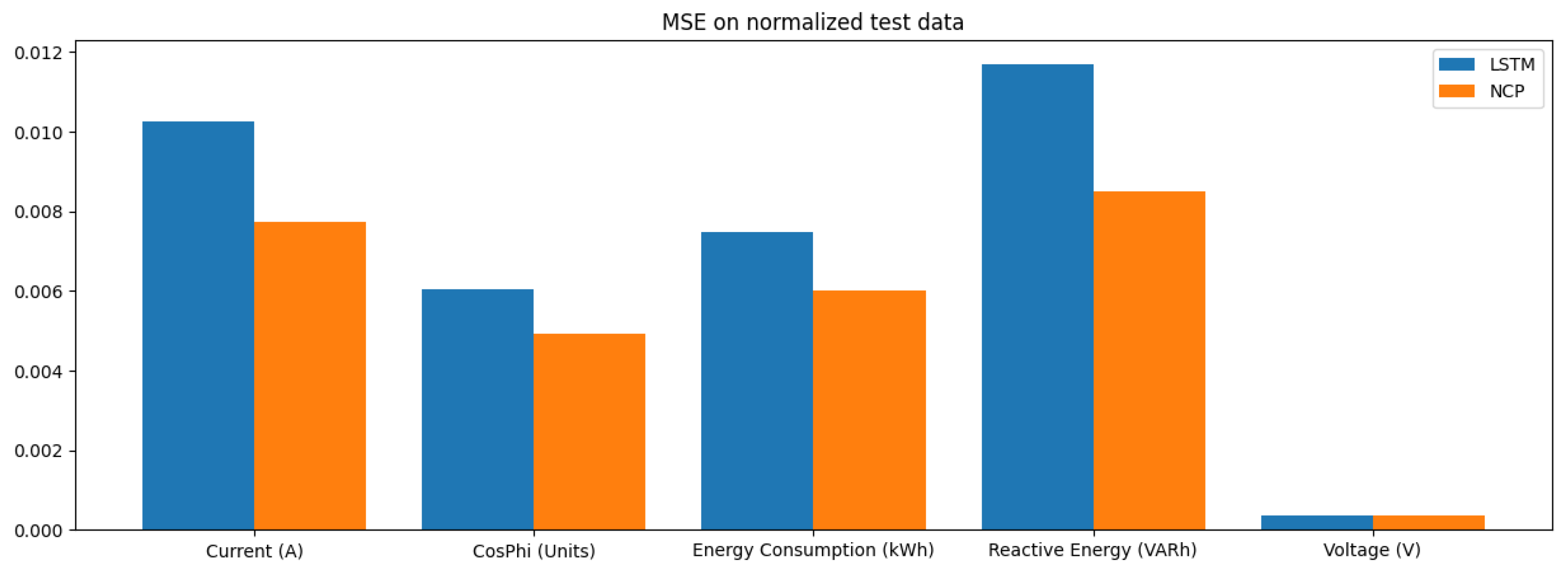
Table 2 presents the MSE values for each model across different operational features. The NCP model achieved the lowest average MSE, indicating its superior predictive accuracy compared to other models.
Table 3 summarizes the MAE for each model across different features. The NCP model again shows a lower average MAE, reinforcing its effectiveness in providing accurate predictions while minimizing error magnitudes.
The RMSE values presented in
Table 4 further illustrate the predictive capabilities of each model across various features, with NCP achieving the lowest average RMSE, indicating its robustness in prediction.
Finally,
Table 5 presents the Coefficient of Determination for each model across different features, highlighting NCP’s superior ability to explain variance in the data.
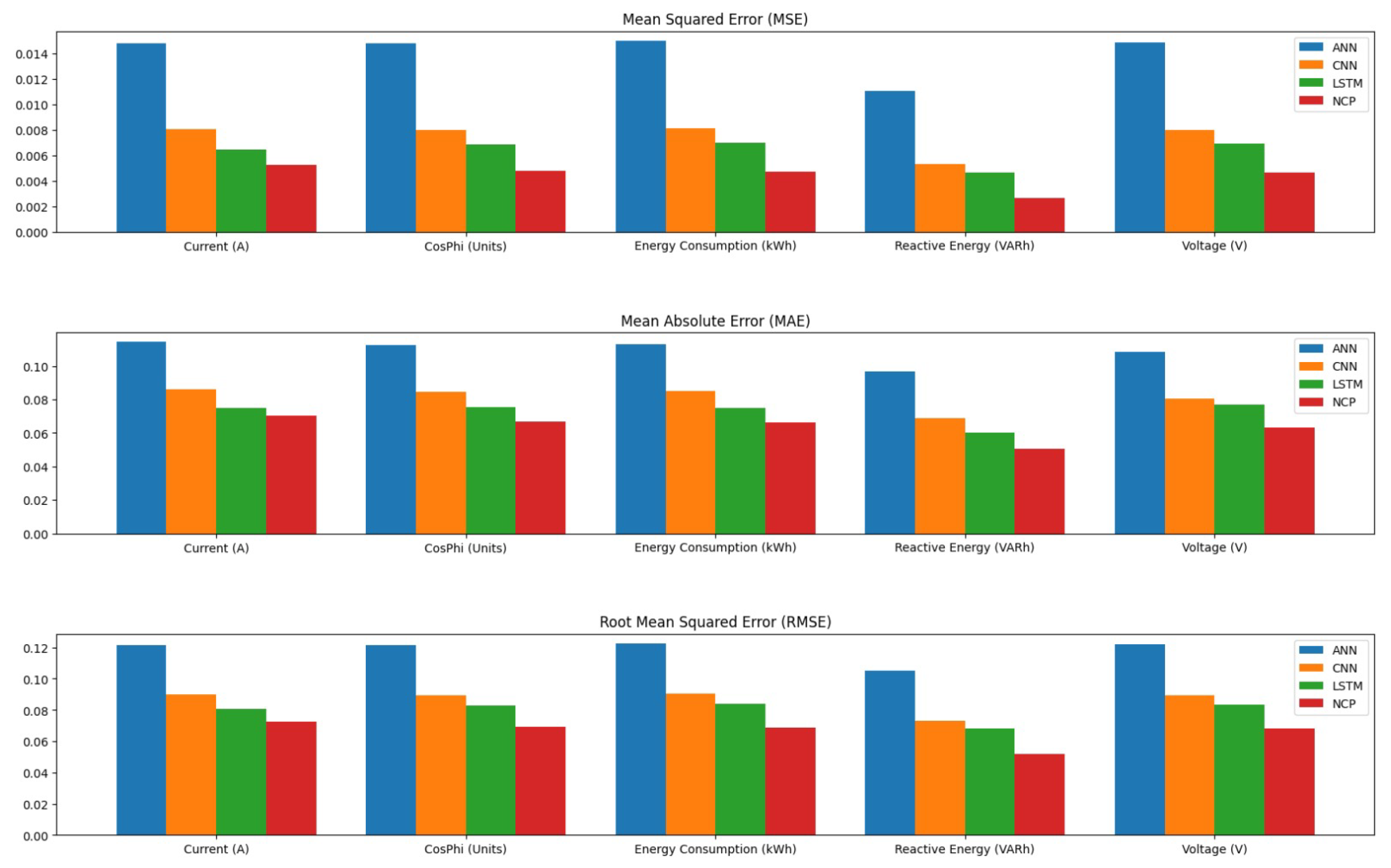
To further illustrate these findings visually, we have included a histogram that summarizes the overall performance metrics across all models in
Figure 14.
The results of our comparative analysis, summarized in
Table 2,
Table 3,
Table 4 and
Table 5, provide valuable insights into the performance of various machine learning models—Neural Circuit Policies, Long Short-Term Memory networks, Convolutional Neural Networks, and Artificial Neural Networks—in detecting anomalies in compressor operations.
In terms of MSE, the NCP model achieved the lowest average MSE of 0.004426, indicating its superior predictive accuracy compared to the other models. The LSTM model followed with an average MSE of 0.006391, while the CNN and ANN models exhibited higher MSE values of 0.007506 and 0.014110, respectively. This trend suggests that the NCP model is more effective in minimizing prediction errors, which is critical in industrial applications where accurate anomaly detection can prevent costly operational failures.
When examining the Mean Absolute Error (MAE), similar patterns emerged. The NCP model again demonstrated the lowest average MAE of 0.063536, signifying that it consistently produces predictions that are closer to the actual values across all features. The LSTM, CNN, and ANN models recorded average MAEs of 0.072605, 0.080926, and 0.108925, respectively. The lower MAE values for NCP indicate its robustness in providing actionable insights for maintenance strategies, reinforcing its potential utility in real-world applications.
The RMSE results further corroborate these findings, with the NCP achieving an average RMSE of 0.066129. This metric, which translates error metrics back into the original units of measurement, allows for a more intuitive understanding of model performance. The LSTM model’s average RMSE was 0.079728, while CNN and ANN models had higher RMSE values of 0.086385 and 0.118598, respectively. The consistent superiority of NCP across all error metrics underscores its effectiveness in capturing the underlying dynamics of compressor operations.
Moreover, the Coefficient of Determination provides insight into how well each model explains the variance in the data. The NCP model achieved an impressive average value of 0.980438, indicating that it explains a significant proportion of variance in operational metrics. In comparison, the LSTM, CNN, and ANN models had average values of 0.971610, 0.966879, and 0.938317, respectively. These results highlight the NCP’s ability to not only predict outcomes accurately but also to provide a comprehensive understanding of the operational dynamics within compressor systems.
To provide a theoretical explanation of the results obtained, we can delve into the mathematical foundations of ANN and CNN architectures.
ANNs operate on the principle of mimicking biological neurons. Each neuron receives input signals, applies a weight to these signals, sums them up, and then passes the result through an activation function. The mathematical representation of a single neuron can be expressed as
where
y is the output;
f is the activation function (e.g., sigmoid, ReLU);
are the weights;
are the input features;
b is the bias term.
The choice of activation function significantly impacts the model’s ability to learn complex patterns. For instance, the ReLU (Rectified Linear Unit) function is defined as
This function allows for faster convergence during training by mitigating the vanishing gradient problem often encountered with sigmoid functions.
CNNs, on the other hand, utilize convolutional layers to automatically extract features from input data, particularly effective for spatial data such as images. The convolution operation can be mathematically represented as
where
The pooling layers that follow convolutional layers reduce dimensionality while preserving essential features. This hierarchical feature extraction allows CNNs to capture spatial hierarchies effectively.
The superior performance of NCPs in our study can be attributed to their ability to integrate physical constraints into the learning process, which enhances their predictive capabilities. In contrast, while both ANNs and CNNs are powerful in capturing complex relationships within data, they may not leverage domain-specific knowledge as effectively as NCPs.
Moreover, NCPs benefit from increased interpretability due to their reliance on established physical laws. The mathematical models used in NCPs often allow for direct insights into system behavior, which is not always possible with black-box models like ANNs and CNNs. This interpretability is crucial in industrial applications where understanding the rationale behind model predictions can inform maintenance strategies and operational decisions.
Thus, while ANNs and CNNs excel at modeling complex non-linear relationships within data through their flexible architectures, they lack the ability to incorporate physical constraints that govern real-world systems. The mathematical formulation of NCPs enables them to produce predictions that are not only accurate but also physically plausible, thereby enhancing their reliability in anomaly detection tasks within industrial contexts.
Moreover, to further illustrate our findings, we present a graph that summarizes the theoretical learning curves of NCPs, ANNs, CNNs, and LSTM networks over training epochs.
Figure 15 displays the accuracy of each model as a function of the number of training epochs.
Analyzing the graphs related to NCPs in comparison to the other three models—ANN, CNN, and LSTM—reveals several significant observations that warrant further exploration.
First and foremost, the overall performance of the NCP model demonstrates a stable convergence behavior for both training loss and evaluation loss, achieving very low values from the first 5–10 epochs. This behavior is similar to that observed in the LSTM model, which also exhibits a rapid decrease in loss during the initial training phases. However, what stands out is the reduced oscillation of losses, particularly evaluation loss, in the NCP model compared to ANN and CNN. This stability suggests that the NCP is capable of maintaining high performance during evaluation, thereby reducing the risk of overfitting and enhancing its ability to generalize on unseen data.
Another important observation pertains to the stability of evaluation loss. Unlike the ANN and CNN, where evaluation loss exhibits more pronounced and unpredictable oscillations, the NCP shows more contained fluctuations. This behavior implies that the NCP has a better capacity to generalize on evaluation data, making it particularly effective in real-world scenarios where data may vary from those used during training.
When comparing NCPs to LSTM, it is noted that both models display similar performance characteristics: both achieve a rapid reduction in loss during the early stages of training. However, the NCP appears to exhibit slightly more regular behavior in evaluation loss. This regularity may indicate a slight superiority in generalization capability for NCP or greater robustness against noise present in the data. This characteristic is especially relevant in industrial applications where operational conditions can be subject to significant variations.
In contrast to LSTM models, both ANNs and CNNs require more time to converge compared to NCPs, taking approximately 20–30 epochs to reach comparable results. The NCP model, on the other hand, achieves a very low loss within just the first 10 epochs. Additionally, both ANNs and CNNs demonstrate greater variability in their losses during training. This variability suggests a potential difficulty for these models in accurately modeling the data or indicates less stability during the training process.
Finally, at the conclusion of training (after 50 epochs), both the NCP and LSTM reach very low final losses for both training and evaluation metrics. This outcome indicates that both models are able to capture the underlying characteristics of the time series data more effectively than the ANN and CNN. The ability to maintain low losses suggests effective learning of the dynamics inherent in the data.
Therefore, the NCP model performs competitively with LSTM, demonstrating slightly superior stability and low losses. It clearly outperforms the ANN and CNN in terms of rapid convergence, stability, and generalization capability. These results highlight that the NCP model is particularly well suited for analyzing time series data within industrial applications.


