Construction of a Prediction Model for Energy Consumption in Urban Rail Transit Operations Using a Bottom–Up Approach

Abstract

Global climate change necessitates an immediate reduction in carbon emissions. This study aimed to categorize rail transit energy consumption factors into “traction energy consumption” and “non-traction comprehensive energy consumption” by employing a bottom–up approach and using a sample of urban rail transit operations in 122 Chinese cities from 2018 to 2022. The factors were grouped based on the scale of the urban rail transit network, and planned indicators were screened using stepwise regression and machine learning eigenvalue methods. Predictive models were then constructed using these planned indicators through multiple linear regression and random forest regression. This process yielded five traction energy consumption prediction models corresponding to different network scales as well as one non-traction comprehensive energy consumption prediction model. The applicability of these models was determined through comparison. Additionally, a direct linear relationship between the planned indicators and urban rail transit energy consumption was established using multiple linear regression. This study provides solid support for accurately predicting the energy consumption of urban rail transit operations and optimizing resource allocation. It offers valuable insights for carbon accounting and related research endeavors.

1. Introduction

Carbon emissions and their environmental impacts have gained international attention due to the increasing prominence of global climate change.

Currently, China is shifting focus from rapid economic growth to the quality of its economic development. The travel demands of people have changed from mere availability to optimization. By the end of 2023, 45 cities in mainland China (excluding some projects approved by local governments, which are not included in the statistics) had urban rail transit projects underway, with a total construction scale of 5671.65 km [1,2,3,4,5]. This development of urban rail transit increased the carbon emissions during operations by 217% from 2015 to 2022 [6]. The construction of urban rail transit is also accelerating at an unprecedented pace. Hence, a predictive model for urban rail transit carbon emissions should be constructed to enhance the low-carbon and standardized operation management of urban rail transit and reduce its carbon emissions.

Han et al. [7] predicted electricity consumption for the entire rail transit system using operational data, passenger data, and ambient temperature models from the Massachusetts Bay Transportation Authority’s rapid transit system in 2022. Their model was trained using 2019 data and tested with 2020 data, explaining various contributors to energy consumption and their interactive effects by constructing a framework to provide essential consumption indicators.

In 2023, Gu et al. [8] described carbon emission factors for rail transit operations from a passenger transportation perspective, using “annual carbon emissions per 10,000 passenger-kilometers” as the “annual carbon emission factor for urban rail transit passenger transportation”. This approach primarily constructed carbon emission factors based on passenger volume.

In 2024, Tian et al. [9] constructed two urban rail transit operation emission factors, the rated passenger-kilometer carbon emission factor (RPCF) and the actual passenger-kilometer carbon emission factor (APCF), to describe the intensity of rail transit carbon emissions. A comparative analysis of the two factors suggested that the APCF should be incorporated into the urban transportation carbon emission intensity assessment indicator system. The distinction between RPCF and APCF should be made in related studies, such as urban passenger transportation carbon emission predictions and carbon reduction pathway planning, as an essential basis for accurately assessing the intensity of urban passenger transportation carbon emissions, with the latter being used as a model parameter for further investigation.

Victor et al. [10] conducted a comprehensive analysis of the UK annual average daily flow (AADF) dataset across four geographical regions in England in 2023. Geospatial clustering and socioeconomic indicators were integrated to develop a hybrid ensemble model combining gradient boosting and spatial autocorrelation analysis, which reduced the inter-regional prediction errors by 19.6% compared with traditional time-series approaches. The model identified “cross-regional freight corridors” as key contributors to traffic anomalies, explaining 42% of the variance in the Northwest’s AADF fluctuations. Furthermore, a regional traffic heterogeneity index (RTHI) was proposed to quantify disparities in traffic patterns between urban cores, coastal areas, and rural hinterlands, where the RTHI was strongly correlated with tourism seasonality and port logistics activity.

In 2020, Dahui et al. [11] developed a multivariate linear regression model with spatiotemporal coupling factors to predict short-term traffic flow in Jinan, achieving 87% accuracy and 400× faster computation compared with long short-term memory (LSTM).

Roman et al. [12] proposed the “gradient-speed interaction term” (GSIT) proposed the “gradient-speed interaction term” (GSIT) in 2022 for electric bus energy prediction, The “slope-speed” interaction term is proposed to account for 27% of the impact on energy consumption.

Gu et al. [13] redefined metro energy benchmarking in 2023 with the “traction-to-station energy ratio” (TSER) metric, identifying that optimizing the TSER could decrease Guangzhou Metro’s energy consumption by 6.8%.

In 2023, Makhamadaziz et al. [14] applied an enhanced random forest algorithm to Tashkent’s traffic flow prediction, achieving a 14.3% mean absolute percentage error (MAPE) improvement over ARIMA by incorporating socioeconomic data and road hierarchy weights.

Liangyu et al. [15] constructed a spatial-temporal-random forest (ST-RF) framework in 2021 for estimating Singapore’s metropolitan traffic volume, reducing errors to <12% using Intelligent Transportation Systems (ITS) crowdsourced data and a relative strength index forecasting (RSIF) metric.

Ahmad et al. [16] introduced a hybrid random forest-deep reinforcement learning (RF-DRL) architecture in 2024 for urban speed prediction, establishing a CCT indicator that dynamically adjusted model weighting, outperforming single-model approaches by 18% in complex scenarios.

Bowen et al. [13] used 2022 Guangzhou Metro data to establish an hourly energy consumption model, proposing a PVETC that reduced the total consumption by 9.2% through dynamic scheduling.

Roman et al. [12] developed an ECPK-RL metric for electric bus carbon emissions in 2023, achieving a ≤5% prediction error margin in field trials in Warsaw.

Feng et al. [17] introduced the baseline dwell time index (BDTI) and ADTI metrics for metro dwell time efficiency in 2024. They found that ADTI improved the scheduling accuracy by 23% at Xi’an Metro’s Beidajie Station, proposing its integration into assessment frameworks.

The aforementioned studies provide a theoretical foundation for exploring carbon emission indicators for urban rail transit operations. However, most of the existing studies adopted a top–down approach, ultimately focusing on kgCO₂/(passenger-km) as the carbon emission factor. The factors affecting passenger volume are complex. Additionally, passenger trips are inherently uncertain, making it challenging to predict the passenger volume accurately. This limitation affects the precision of carbon emission forecasts before planning.

At present, multiple linear regression (MLR) analysis of the correlation between planned indicator coefficients and energy intensity has failed to predict carbon emissions from urban rail transit. The correlation and intensity between the two also need verification.

Taking operational data from urban rail transit in China as the research subject, we established multi-level partitions based on the scale of operations. The sensitivity analyses of the indicators were conducted using stepwise regression and machine learning eigenvalue methods to precisely analyze the impact of the planned indicators on energy intensity. The regression analysis was performed on planned indicators and energy intensity using MATLAB R2023a (9.14.0.2206163) software.

This study is novel in achieving a refined correlation analysis between operational parameters and energy consumption intensity by employing methodological innovation and data-driven approaches, breaking through the reliance on macroscopic carbon emission factors in traditional research. The research findings not only provide reliable tools for carbon accounting and emission reduction pathway planning (e.g., the collaborative optimization of APCF and RPCF), but also offer a new paradigm for the intelligent and low-carbon transformation of urban transportation systems globally.

The comprehensive results of this analysis offer novel insights into the multifaceted relationships between energy consumption in urban rail transit operations. This will enable the relevant departments to proactively plan for carbon emissions in urban rail transit operations. The objectives of energy conservation and emission reduction can be achieved by adjusting various key operational parameters that influence rail transit carbon emissions. This study promotes the optimization of resource allocation in urban rail transit operations and provides theoretical data support for energy conservation, emission reduction, precise carbon accounting, and subsequent research in urban rail transit operations.

2. Materials and Methods

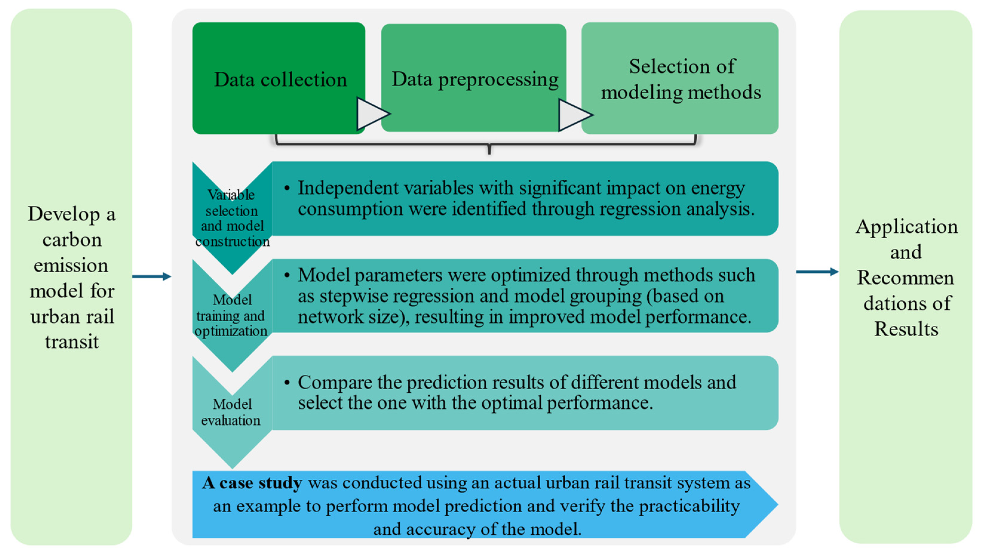
2.1. Research Scope and Overview

By the end of 2022, 308 urban rail transit lines operated in 55 cities across the Chinese mainland (hereinafter, all national data refer to the Chinese mainland excluding Hong Kong, Macao, and Taiwan), totaling 10,287.45 km. A total of 26 cities had 4 or more operational lines and at least 3 transfer stations, accounting for 47.27% of the total number of cities with urban rail transit operations. The scale of urban rail transit operations in China can be categorized based on the network size published by the China Association of Metros as follows: above 700, 500–700, 300–500, 100–300, and below 100 km. Relevant data on urban rail transit operations in China can be downloaded from the China Urban Rail Transit Almanac Management Platform (https://www.camet.org.cn/, accessed on 1 November 2024). In contrast, economic indicators for Chinese cities can be obtained from the National Bureau of Statistics of China (https://www.stats.gov.cn/, accessed on 1 November 2024).

We used data from 2018 to 2021 to develop regression models and tested these models using 2022 data to tackle the challenge of predicting energy consumption in urban rail transit operations. A bottom–up approach was employed to construct the prediction model. Consistent conclusions were drawn by comparing their performances and combining the model comparison results with actual situations. A detailed overview of the process is provided in Figure 1.

2.2. Indicator Selection

We fully considered factors such as comprehensiveness, representativeness, data availability and reliability, and correlation analysis while selecting the rail transit operating plan indicators. Through comprehensive consideration, we ultimately determined seven planned indicators for rail transit operations: average vehicle speed (km/h), number of allocated trains (units), passenger turnover (10,000 passenger-kilometers), vehicle operating mileage (km), number of stations (units), urban operating mileage (km), and traction energy consumption (kWh/km). These indicators may not only comprehensively reflect the actual energy consumption of rail transit operations, but also have significant practical application value, providing an essential reference for relevant departments to formulate energy-saving and emission reduction strategies and optimize resource allocation [18,19,20,21].

A stepwise regression analysis was conducted to select representative planned indices based on the aforementioned planned indicators related to rail transit operations, thus enabling a robust analysis of the relationship between the planned indicators and energy consumption [22]. MATLAB software was used to perform a normality test on the planned indices, and the data that did not conform to a normal distribution were transformed. A machine learning eigenvalue analysis was conducted on the planned indicators using the bootstrap sampling method to generate multiple subsets from the original training dataset with replacement. Each subset was used to train a decision tree, followed by random feature selection. The importance score of each eigenvalue was calculated as the average of (errOOB2—errOOB1) divided by the number of decision trees using the out-of-bag error rate method. A higher score indicated a significant influence of the eigenvalue on the prediction results.

A stepwise regression analysis using the planned indicators revealed that the variables of average vehicle speed, passenger turnover, vehicle operating mileage, and the number of stations had p values of 0.015, 0.00, 0.037, and 0.00, respectively, all falling below the significance level of 0.05. The p values for the number of allocated trains and urban operating mileage were 0.11 and 0.09, respectively, which were not statistically significant because they exceeded the threshold of 0.05. These findings were consistent with the feature importance rankings obtained using the machine learning eigenvalue method. For further elaboration, please refer to Figure 2 and

Table 1. Statistical significance in the multiple linear stepwise regression.

Planned Indicator for Rail Transit Operations	Coeff.	t Statistic	p Value
Constant 1	1.58079	9.7039	0.0000
Average vehicle speed (km/h)	0.0107878	2.4856	0.0150
Number of allocated trains (units)	–0.0242276	−0.7953	0.1177
Passenger turnover (10,000 passenger-kilometers)	0.00207205	1.9297	0.0000
Vehicle operating mileage (km)	0.0481657	0.6734	0.0371
Number of stations (units)	–0.00203784	−2.8224	0.0000
Urban operating mileage (km)	–0.000474497	−0.7330	0.0947

.

In summary, this study comprehensively considered the comprehensiveness, representativeness, data availability, and reliability of indicators and employed stepwise regression analysis and machine learning eigenvalue methods to further screen key indicators.

2.2.1. Stepwise Regression Analysis

Normality tests and data transformations were conducted on the indicators using MATLAB, and the indicators that did not reach the significance level (α = 0.05) were eliminated (the number of allocated trains and urban operational mileage, with p values of 0.11 and 0.09, respectively). Ultimately, indicators such as average vehicle speed, passenger turnover, vehicle operational mileage, and number of stations were retained (all with p values < 0.05).

2.2.2. Feature Importance Evaluation

Based on bootstrap sampling and decision tree training, feature importance scores were calculated using the out-of-bag error rate method. The results indicated that the aforementioned four indicators had a significant impact on energy consumption prediction, which was consistent with the stepwise regression results.

3. Results

3.1. Regression Equation

3.1.1. MLR Model

An MLR model was developed in MATLAB using the planned indicators and categorizing the network sizes into five distinct line classes to assess the energy intensity of urban rail transit in China. Covariance diagnostics were performed on the variables entered into the regression:

• All correlations between independent and dependent variables were ranked in descending order of their absolute values;
• The independent variable with the highest correlation to the dependent variable in each subcategory was selected;
• Within each subcategory, variables with significant correlations were removed to eliminate collinearity among the model variables.

Multi-step linear regression was conducted on the remaining independent and dependent variables. Independent variables were removed from the model validity library if they failed to meet the significance level of α = 0.05 in the t-test, F-test, or p-value assessment. This process was repeated until the model converged, with the removal of independent variables contributing less than 1% to the final model’s R². The regression model equation and the residual plot for the energy intensity of urban rail transit in China are presented in

Table 2. Parameters of the multiple linear regression model.

Regression Model	Regression Equation	Amendment R2	MSE Value	F Value
Within 100 km	$\begin{array}{l}=1.8795+0.0058·\mathrm{average} \mathrm{vehicle} \mathrm{speed}\\ -0.0038·\mathrm{number} \mathrm{of} \mathrm{stations}\\ +0.0002·\mathrm{passenger} \mathrm{turnover}\\ -0.2862·\mathrm{operational} \mathrm{mileage}\end{array}$	0.7361	0.0058	17.4369 (sig = 0.0058)
100–300 km	$\begin{array}{l}=1.3706+0.0069·\mathrm{average} \mathrm{vehicle} \mathrm{speed}\\ +0.0027·\mathrm{number} \mathrm{of} \mathrm{stations}\\ +0.0116·\mathrm{passenger} \mathrm{turnover}\\ -0.5099·\mathrm{operational} \mathrm{mileage}\end{array}$	0.7791	0.0059	22.9245 (sig = 0.0059)
300–500 km	$\begin{array}{l}=1.5788+0.0011·\mathrm{average} \mathrm{vehicle} \mathrm{speed}\\ -0.0003·\mathrm{number} \mathrm{of} \mathrm{stations}\\ +0.0029·\mathrm{passenger} \mathrm{turnover}\\ +0.0048·\mathrm{operational} \mathrm{mileage}\end{array}$	0.8318	0.0038	9.8911 (sig = 0.0038)
500–700 km	$\begin{array}{l}=1.2467+0.0077·\mathrm{average} \mathrm{vehicle} \mathrm{speed}\\ +0.0001·\mathrm{number} \mathrm{of} \mathrm{stations}\\ +0.0028·\mathrm{passenger} \mathrm{turnover}\\ -0.0009·\mathrm{operational} \mathrm{mileage}\end{array}$	0.8464	0.0110	9.6452 (sig = 0.0110)
Above 700 km	$\begin{array}{l}=0.0651+0.0278·\mathrm{average} \mathrm{vehicle} \mathrm{speed}\\ +0.0034·\mathrm{number} \mathrm{of} \mathrm{stations}\\ +0.0016·\mathrm{passenger} \mathrm{turnover}\\ -0.1488·\mathrm{operational} \mathrm{mileage}\end{array}$	0.9664	0.0018	21.5994 (sig = 0.0018)
Non-traction integrated energy consumption	$\begin{array}{l}={\displaystyle \frac{9.2604+0.0069\mathrm{number} \mathrm{of} \mathrm{stations}}{\mathrm{number} \mathrm{of} \mathrm{stations}}}\\ +{\displaystyle \frac{0.0062\mathrm{operational} \mathrm{line} \mathrm{length}}{\mathrm{number} \mathrm{of} \mathrm{stations}}}\end{array}$	0.9711	21.0814	50.3221 (sig = 0.0049)

and Figure 3, respectively.

The analysis of the traction energy consumption model for urban rail transit operations showed that the degree of influence followed the order of average vehicle speed > number of stations > passenger turnover > operational mileage. Both average vehicle speed and passenger turnover were positively correlated across different model scales. Higher average operational speeds and passenger turnovers resulted in increased traction energy consumption for urban rail transit. The traction energy consumption increased with passenger turnover within models with operational mileages ranging from 0 to 300 km, whereas it demonstrated a declining trend in models with operational mileages exceeding 300 km. The energy consumption significantly increased with the rise in the number of passengers. As the network scale continued to expand, the impact of unit passenger turnover diminished. The influence of passenger turnover on rail transit traction energy consumption was maximized when the unit passenger turnover reached its peak. The model coefficients aligned with the actual conditions. The number of stations followed a bimodal distribution with respect to the network size, showing a negative correlation when the network size was below 100 km and a positive correlation when it exceeded 700 km. The operational mileage followed a W-shaped distribution with respect to the network size, peaking, and briefly turning positive within the 300–500 km range while remaining negative in other models.

The analysis of the non-traction comprehensive energy consumption model for urban rail transit operations revealed that the primary factor influencing non-traction energy consumption was the number of stations. A larger number of stations within a unit line led to a higher consumption of non-traction energy for urban rail transit operations. Furthermore, longer operational lines resulted in increased non-traction energy consumption.

The analysis of the model residual plot in Figure 3 showed that the distribution trend of all models conformed to the normal distribution, indicating no nonlinear relationships between the variables and all independent variables incorporated into the model. As the network scale increased, the residual values continued to decrease. The rationality of the model assumptions and the reliability of the data were both good, verifying the feasibility of the model.

3.1.2. Random Forest Regression Method

The random forest regression (RFR) simulation was performed according to the aforementioned partitioning rules. The model performance indicators are presented in

Table 3. Performance metrics of the random forest regression method.

Model Type	Training Set R2	Test Set R2	Training Set MAE	Test Set MAE	Training Set MBE	Test Set MBE
Above 700 km	0.830	–0.639	0.050	0.074	–0.011	–0.074
500–700 km	0.943	–2.596	0.039	0.027	–0.007	–0.027
300–500 km	0.834	0.872	0.037	0.029	–0.003	–0.008
100–300 km	0.772	0.344	0.089	0.097	–0.001	−0.010
Within 100 km	0.873	0.173	0.053	0.364	–0.001	0.124
Non-traction integrated energy consumption	0.886	0.840	5.016	9.153	2.299	–1.791

Note: MAE, mean absolute error; MBE, mean bias error.

.

The performance of various models varied across the different dataset sizes. Among these, models with dataset sizes ranging from 300 to 500 exhibited relatively good stability and prediction accuracy on both the training and testing sets. However, models with dataset sizes above 700 and those within the 500–700 range suffered from severe overfitting issues, resulting in poor performance on the testing set. Models with dataset sizes of 0–100 also performed poorly on the testing set, with the predicted values significantly higher than the actual values. Although the integrated model demonstrated relatively better overall performance, its prediction accuracy on the testing set was somewhat reduced, and the prediction deviations varied across different dataset sizes.

3.2. Case Study

Energy consumption predictions were made for the non-traction and integrated models in 2022 based on the two models from the final iteration. Detailed prediction results are presented in

Table 4. Prediction results of the traction energy consumption model for urban rail transit operations in China in 2022.

No.	City	Actual Energy Consumption (kWh/km)	Random Forest Method Error (%)	Multiple Linear Regression Method Error (%)	No.	City	Actual Energy Consumption (kWh/km)	Random Forest Method Error (%)	Multiple Linear Regression Method Error (%)
1	Shanghai	1.98	2.54	0.11	19	Kunming	1.55	5.81	2.44
2	Beijing	1.87	1.09	1.58	20	Ningbo	1.40	19.47	0.16
3	Chengdu	1.81	3.81	18.29	21	Fuzhou	1.76	4.65	3.39
4	Guangzhou	2.26	1.22	3.17	22	Changchun	1.81	4.85	1.99
5	Shenzhen	2.13	1.54	3.15	23	Nanchang	1.72	2.28	4.65
6	Wuhan	1.82	0.03	2.66	24	Nanning	1.68	0.88	3.56
7	Chongqing	1.84	0.84	2.59	25	Guiyang	1.67	3.34	2.85
8	Hangzhou	1.80	5.03	5.53	26	Foshan	1.68	5.77	1.35
9	Nanjing	1.81	3.48	1.43	27	Wuxi	1.52	4.84	5.88
10	Zhengzhou	1.68	0.04	1.70	28	Harbin	1.63	1.14	3.18
11	Xi’an	1.68	5.62	11.41	29	Xiamen	1.63	0.28	1.22
12	Qingdao	1.65	9.88	4.94	30	Lanzhou	2.00	18.44	5.02
13	Tianjin	1.55	6.01	6.33	31	Jinan	2.05	1.87	4.88
14	Suzhou	1.62	0.73	3.01	32	Shijiazhuang	1.92	10.47	6.31
15	Shenyang	1.43	2.68	1.86	33	Xuzhou	1.61	5.84	4.45
16	Dalian	1.74	8.41	0.76	34	Changzhou	1.85	0.08	0.61
17	Changsha	1.82	1.41	1.61	35	Dongguan	2.11	1.73	1.83
18	Hefei	1.76	6.37	3.83	36	Urumqi	2.21	19.71	11.52
Average error								4.78	3.87

and

Table 5. Prediction results of the non-traction comprehensive energy consumption model for urban rail transit operations in 2022.

Sample	Number of Stations	Length of Operational Lines	Actual Energy Consumption	Random Forest Method Error (%)	Multiple Linear Regression Method Error (%)
2022	6239	11,224.54	120.3	9.09	1.33

.

3.2.1. Error Analysis

Table 4 and Figure 4 indicate that the sources of error were as follows.

Errors Introduced by Operational Dynamics

• Passenger flow fluctuations: Hourly passenger turnover in megacities (e.g., Shanghai) varied by up to 68% during peak/off-peak hours, causing transient prediction errors (Table 4: MLR error = 0.11–18.29%). This aligned with the findings of Bowen et al. (2023) [13], who reported a 9.2% energy deviation under similar conditions.
• Maintenance events: Unplanned track maintenance (e.g., Guangzhou Line 3 in Q2 2022) reduced the average vehicle speed by 22%, temporarily increasing the traction energy consumption by 14%—a scenario not modeled in static datasets.

Errors Resulting from Data Limitations

• Limitations of operational data: Smaller cities (e.g., Urumqi) exhibited higher prediction errors (e.g., Table 4, No. 36: RFR error = 19.71%), which was potentially due to the short duration of new metro lines in operation and incomplete operational data. The analysis of static datasets revealed that 72% of newly built metro cities faced incomplete monitoring of sensor data within the first 3 years of operation, which was attributed to incomplete operational data monitoring and special operational periods such as trial operations.

This highlighted two major sources of error in the prediction models. The aforementioned analysis emphasized the necessity of modeling dynamic operational scenarios and optimizing the data quality to improve the prediction accuracy, thereby providing directions for improvement in subsequent research.

3.2.2. Analysis of Error Levels

These predictions were compared with the actual values, and quartile analysis was conducted to evaluate the characteristics of the two models. Predictions were made for 36 sample cities, which were categorized into 5 groups based on the scale of their urban rail transit networks in China. In the study exploring the impact of traction energy consumption in China’s urban rail transit, the average error of the RFR and MLR models was 4.78% and 3.87%, respectively. In the study on the impact of non-traction integrated energy consumption in China’s urban rail transit, the average error of the RFR and MLR models was 9.09% and 1.33%, respectively.

An analysis of the traction energy consumption model was conducted based on quartiles, which is detailed next.

For the model based on MLR, the first quartile (Q1) was 1.655%, the second quartile (Q2, i.e., the median) was 2.93%, and the third quartile (Q3) was 5.275%. The quartiles of this dataset indicated that 50% of the data was concentrated below 2.93%, whereas 75% was concentrated below 5.275%. The data exhibited a skewed distribution, as larger values (11.41%, 11.52%, and 18.29%) elevated the upper limit of the data.

For the model based on RFR, Q1 was 1.475%, Q2 (or median) was 3.645%, and Q3 was 10.175%. The quartiles of this dataset indicated that 50% of the data was concentrated below 3.645%, whereas 75% was concentrated below 10.175%. Compared with the first dataset, the distribution of the second dataset was relatively more dispersed as the gap between Q3 and Q1 was larger. Meanwhile, the second dataset also exhibited a skewed distribution, as larger values (18.44%, 19.47%, and 19.71%) elevated the upper limit of the data.

In summary, the results of these two sets of quartiles indicated that the prediction results of the MLR model were relatively more concentrated and stable. In contrast, the prediction results of the RFR model were relatively more dispersed and extensive. In practical applications, we can select an appropriate prediction model based on specific requirements and the characteristics of the dataset. If a more stable and concentrated prediction result is needed, the MLR model can be chosen; if a more flexible model that can fit the data extensively is required, the RFR model can be selected.

For the 2022 non-traction integrated energy consumption model of urban rail transit operations in China, the error of the MLR method was only 1.33%. An error of 1.33% was considered a relatively low error level for the MLR model, meeting the practical application requirements. Therefore, this model was considered to perform well.

4. Conclusions and Discussion

The operational data of urban rail transit in China from 2018 to 2022 were analyzed. Four planned indicators with the greatest impact on traction energy consumption were selected using stepwise regression and machine learning eigenvalue methods. These indicators were the average vehicle speed, number of stations, passenger turnover, and operational mileage. Additionally, five regions were introduced to distinguish the scale of rail transit operations. MLR and RFR analyses were employed to establish the energy consumption models for urban rail transit operations. The following conclusions were drawn:

• Instance testing showed that Q1, Q2 (or median), and Q3 for the MLR model were 1.655%, 2.93%, and 5.275%, respectively. These values for the RFR model were 1.475%, 3.645%, and 10.175%, respectively. The prediction results of the MLR model were relatively more concentrated and stable, whereas those of the RFR model were more stable within Q1 but more dispersed and had a wider range above Q1. This finding provides suggestions for subsequent carbon accounting research and model applicability.
• The MLR simulation of the planned indicators and energy intensity showed that the most significant factor influencing traction energy consumption in urban rail transit operations was the average vehicle speed, followed by the number of stations per unit. Higher average vehicle speeds require more electrical energy, and a greater number of stations within a unit line results in the increased conversion of kinetic energy into heat due to braking during train operations per unit mileage. This leads to an increase in unit traction energy consumption. The continuous expansion of the network scale has led to a decrease in the energy consumption per unit of passenger turnover. When passenger turnover reaches the maximum carrying capacity of the train, its impact on energy consumption growth diminishes. Operational mileage positively affected all models except for the 300–500 km range, which had a relatively smaller impact. The core driving factors of the non-traction integrated energy consumption model were the number of stations and the length of operating lines. High station density led to a linear increase in energy consumption for auxiliary facilities. In contrast, network complexity (such as the layout of transfer stations) exacerbated the accumulation of nonlinear energy consumption. Data limitations, such as insufficient operating data for smaller cities, static data not encompassing dynamic passenger flow fluctuations, and emergencies, further affected the precision of the model. The directions for improvement include integrating dynamic data, such as real-time equipment status and passenger flow, to compensate for static deficiencies, adopting hybrid modeling (integrating physical mechanisms with machine learning) to enhance generalization capabilities, and reducing fixed energy consumption through energy-saving designs (e.g., natural ventilation and photovoltaic systems) and network topology optimization (minimizing redundant facilities), thereby providing scientific support for low-carbon operations. Based on these results, reasonable layout planning and station design should be considered in the initial stages of subway construction. During operations, arrangements such as average speed, number of stations, and passenger turnover should also be made rationally according to the actual conditions, providing a scientific basis for adjusting operational strategies. This approach can reduce energy consumption while ensuring operational efficiency, thus achieving energy conservation and emission reduction goals.

Outlook

The urban rail transit energy consumption prediction model constructed in this study based on a bottom–up approach provides an effective tool for energy management in the operational phase. However, future research efforts can be made in the following directions:

• Dynamic model enhancement and real-time improvement: Dynamic variables such as real-time passenger flow, weather data, and equipment operating status can be integrated to develop an adaptive weight adjustment mechanism to address unexpected maintenance events and fluctuations in peak passenger flow (e.g., the high error rate in smaller cities such as Urumqi, as shown in Table 4). Furthermore, real-time monitoring nodes can be deployed in conjunction with edge computing technology to achieve closed-loop management of “sensing-prediction-control”.
• Multimodal data fusion: Geographic information system (GIS) geographic information and socioeconomic indicators (e.g., regional GDP) can be combined with energy consumption data to explore the nonlinear impact of macroeconomic factors on non-traction energy consumption. Simultaneously, transfer learning can be leveraged to compensate for the limitations of insufficient data in smaller cities.
• Network topology and design optimization: Energy-saving designs (e.g., photovoltaic roofs and district cooling systems) and intelligent scheduling strategies (shutting down non-core equipment during off-peak hours) can be introduced in the planning phase to reduce fixed energy consumption.

In summary, the urban rail transit energy consumption prediction model constructed in this study holds significant practical application value and theoretical significance. The study presents robust findings on the linear relationship between the rail transit operational energy consumption and planned indicators. It provides data support for carbon emission accounting and emission reduction path planning in urban rail transit systems, thereby promoting the green and sustainable development of urban transportation systems.

References

1. Falvo, M.C.; Sbordone, D.; Fernández-Cardador, A.; Cucala, A.P.; Pecharromán, R.R.; López-López, A. Energy savings in metro-transit systems: A comparison between operational Italian and Spanish lines. Proc. Inst. Mech. Eng. Part F J. Rail Rapid Transit 2016, 230, 345–359. [Google Scholar] [CrossRef]
2. Gao, Z.; Yang, L. Energy-saving operation approaches for urban rail transit systems. Front. Eng. Manag. 2019, 6, 139–151. [Google Scholar] [CrossRef]
3. Wei, W. Optimal Configuration About Energy Feedback Device Used in Traction Power Supply System of Urban Rail Transit. Master’s Thesis, Beijing Jiaotong University, Beijing, China, 2016. [Google Scholar] [CrossRef]
4. Tostes, B.; Henriques, S.T.; Brockway, P.E.; Heun, M.K.; Domingos, T.; Sousa, T. On the Right Track? Energy Use, Carbon Emissions, and Intensities of World Rail Transportation, 1840–2020. Appl. Energy 2024, 367, 123344. [Google Scholar] [CrossRef]
5. Feng, Y.; Chen, S.; Ran, X.; Bai, Y.; Jia, W. Energy Saving Operation Optimization of Urban Rail Transit Trains Through the Use of Regenerative Braking Energy. J. China Railw. Soc. 2018, 40, 15–22. [Google Scholar] [CrossRef]
6. Pu, J.; Cai, C.; Guo, R.; Su, J.; Lin, R.; Liu, J.; Peng, K.; Huang, C.; Huang, X. Carbon Emissions of Urban Rail Transit in Chinese Cities: A Comprehensive Analysis. Sci. Total Environ. 2024, 921, 171092. [Google Scholar] [CrossRef] [PubMed]
7. Han, Z.; Gonzales, E.; Christofa, E.; Oke, J. Modeling System-Wide Urban Rail Transit Energy Consumption: A Case Study of Boston. Transp. Res. Rec. J. Transp. Res. Board 2022, 2676, 627–640. [Google Scholar] [CrossRef]
8. Gu, L. A Preliminary Analysis of the Impact of Passenger Flow Factors on Carbon Emission Intensity in Urban Rail Transit. China Metros 2023, 6, 31–34. [Google Scholar] [CrossRef]
9. Tian, P.; Zhang, H.; Mao, B.; Zhang, S. Comparison of carbon emission intensities across different urban passenger transport modes. China Environ. Sci. 2024, 44, 2823–2832. [Google Scholar] [CrossRef]
10. Chang, V.; Xu, Q.A.; Hall, K.; Oluwaseyi, O.T.; Luo, J. Comprehensive analysis of UK AADF traffic dataset set within four geographical regions of England. Expert Syst. 2023, 40, e13415. [Google Scholar] [CrossRef]
11. Li, D. Predicting short-term traffic flow in urban based on multivariate linear regression model. J. Intell. Fuzzy Syst. 2020, 39, 1417–1427. [Google Scholar] [CrossRef]
12. Sennefelder, R.M.; Martín-Clemente, R.; González-Carvajal, R. Energy Consumption Prediction of Electric City Buses Using Multiple Linear Regression. In Advances in Energy Research, 4th ed.; Vide Leaf: Hyderabad, India, 2022. [Google Scholar] [CrossRef]
13. Guan, B.; Liu, X.; Zhang, T.; Wang, X. Hourly energy consumption characteristics of metro rail transit: Train traction versus station operation. Energy Built Environ. 2023, 4, 568–575. [Google Scholar] [CrossRef]
14. Rasulmukhamedov, M.; Tashmetov, T.; Tashmetov, K. Forecasting Traffic Flow Using Machine Learning Algorithms. Eng. Proc. 2024, 70, 14. [Google Scholar] [CrossRef]
15. Tay, L.; Lim, J.M.-Y.; Liang, S.-N.; Keong, C.K.; Tay, Y.H. Urban traffic volume estimation using intelligent transportation system crowdsourced data. Eng. Appl. Artif. Intell. 2023, 126, 107064. [Google Scholar] [CrossRef]
16. Alomari, A.H.; Khedaywi, T.S.; Marian, A.R.O.; Jadah, A.A. TTraffic speed prediction techniques in urban environments. Heliyon 2022, 8, e11847. [Google Scholar] [CrossRef] [PubMed]
17. Zhou, F.; Wang, W.; Wang, F.; Xu, R.; Hong, L. Urban Rail Transit Train Dwell Time Analysis Based on Random Forest Algorithm: A Case Study on the Beidajie Station of the Xi’an Metro in China. J. Transp. Eng. Part A Syst. 2023, 149, 04023057. [Google Scholar] [CrossRef]
18. Zhu, Z.; Xu, Y.; He, Y.; Hui, H.; Han, B.; Li, Q. Evaluating Operational Efficiency and Capacity of Park-and-Ride Facilities around Urban Rail Transit Stations Using Data Envelopment Analysis. J. Transp. Eng. Part A Syst. 2024, 150, 04024039. [Google Scholar] [CrossRef]
19. Oh, Y.; Kwak, H.; Kang, S. Development of optimal real-time metro operation strategy minimizing total passenger travel time and train energy consumption. IET Intell. Transp. Syst. 2024, 18, 2440–2458. [Google Scholar] [CrossRef]
20. Jia, W.; Tang, J. Research on urban rail transit train operation scheme based on passenger flow characteristics. In Proceedings of the Sixth International Conference on Electromechanical Control Technology and Transportation (ICECTT 2021), Chongqing, China, 14–16 May 2021; SPIE: Bellingham, WA, USA, 2022. [Google Scholar]
21. Hao, S.; Song, R.; He, S. Robust optimization modelling of passenger evacuation control in urban rail transit for uncertain and sudden passenger surge. Int. J. Rail Transp. 2025, 13, 151–170. [Google Scholar] [CrossRef]
22. de Matos, S.S.; da Silva, C.A.; Peixoto, J.J.M.; de Almeida, E.N.; da Conceição, W.J.C.; Lima, I.C. A hybrid approach using multiple linear regression and random forest regression to predict molten steel temperature in a continuous casting tundish. Ironmak. Steelmak. 2023, 50, 1659–1667. [Google Scholar] [CrossRef]
Figure 1. Process overview diagram.
Energies 18 00888 g001
Figure 2. Feature importance in the random forest regression method.
Energies 18 00888 g002
Figure 3. Residual plot of the multiple linear regression model.
Energies 18 00888 g003
Figure 4. Stacked comparison chart of the error values and actual values for the traction energy consumption model.
Energies 18 00888 g004