
Integrated Phase-Change Materials in a Hybrid Windcatcher Ventilation System


Abstract
1. Introduction
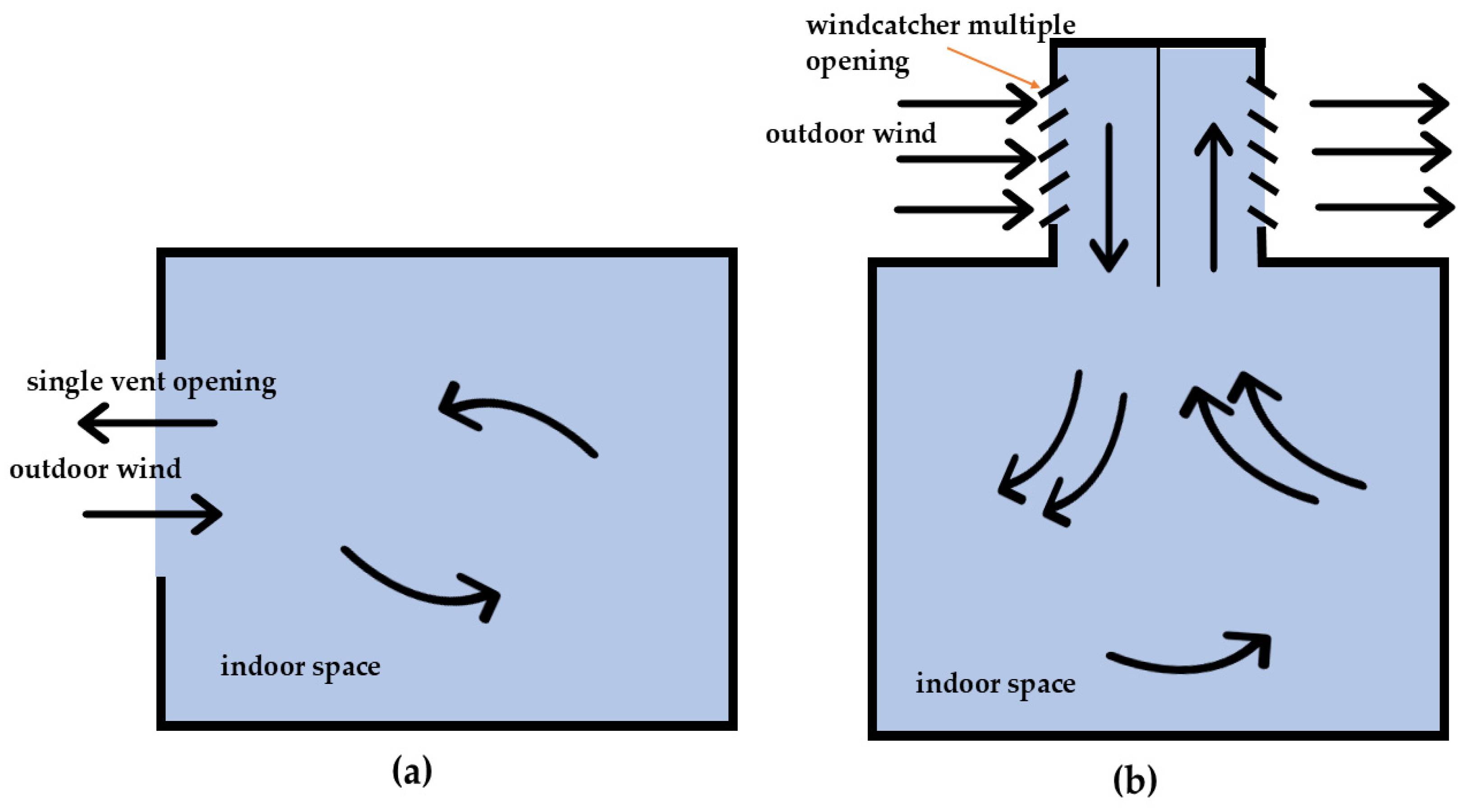
1.1. Windcatchers
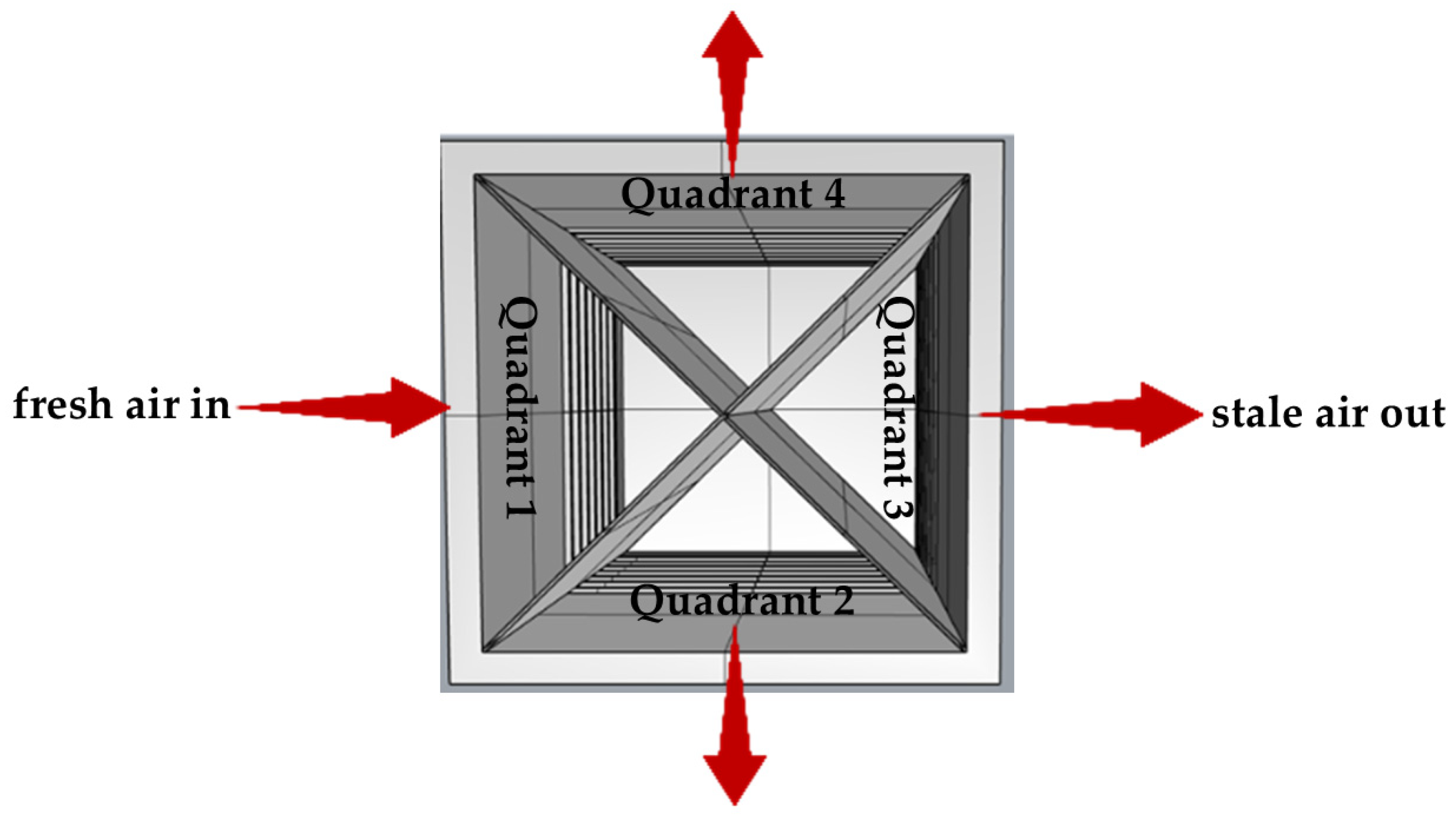
1.2. Multidirectional Windcatcher Passive Ventilation
1.2.1. Effect of Wind Speeds on Windcatcher Ventilation
1.2.2. Effect of Wind Angles on Windcatcher Ventilation
1.3. Fan-Assisted Windcatcher Hybrid Ventilation
1.4. Integrating Passive Cooling Devices with Windcatchers
1.4.1. Heat Pipe Integration with Windcatchers
1.4.2. PCMs—Thermal Energy Storage Integration with Windcatchers
1.5. Gap in Knowledge, Novelty, and Aims
- ▪
- How can encapsulated PCMs be optimally integrated into hybrid multidirectional windcatchers to improve both cooling and thermal energy storage performance without compromising overall ventilation effectiveness?
- ▪
- What influence will variations in wind speed and angle have on the system’s cooling, thermal energy storage, and overall ventilation performance?
2. Methods
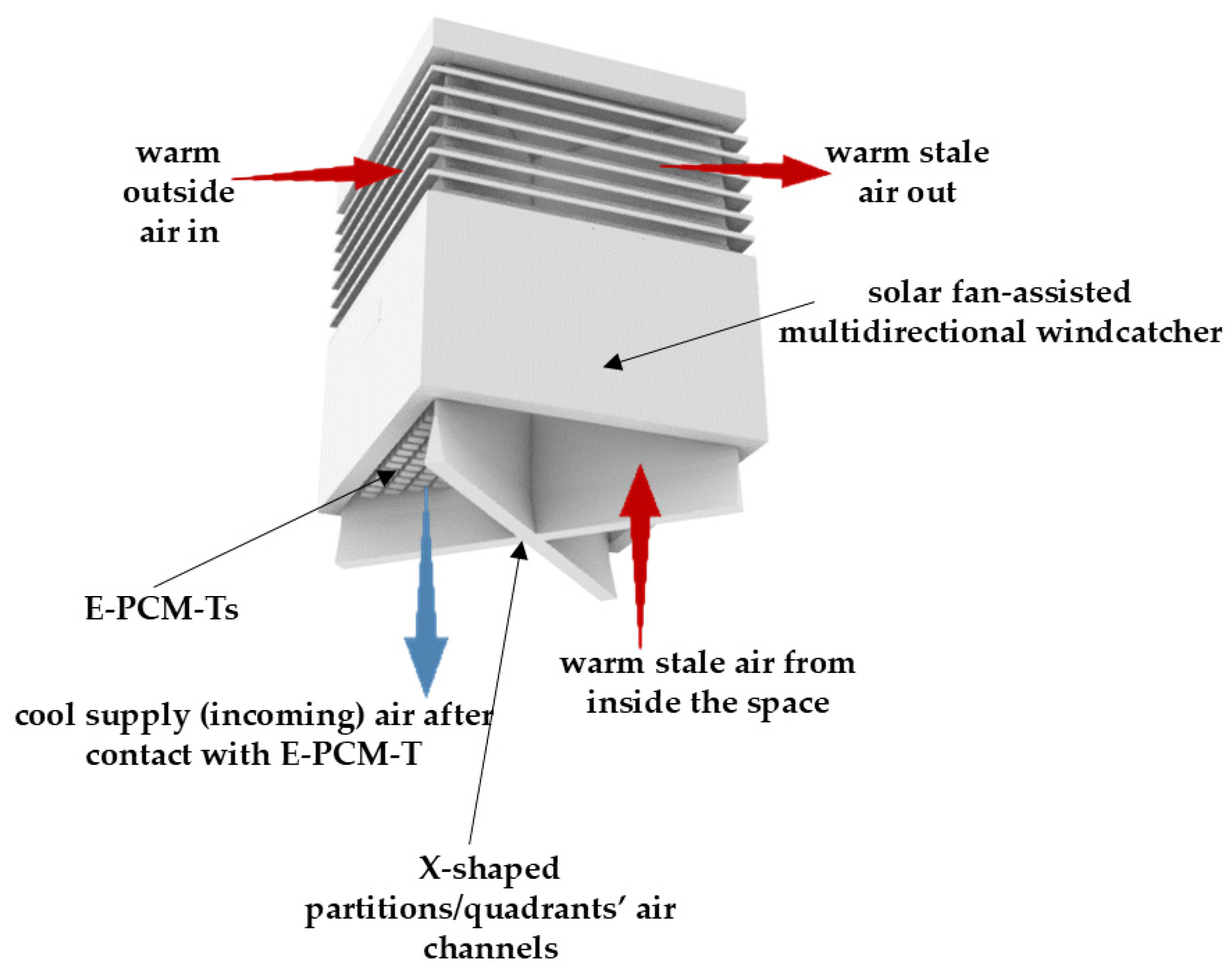
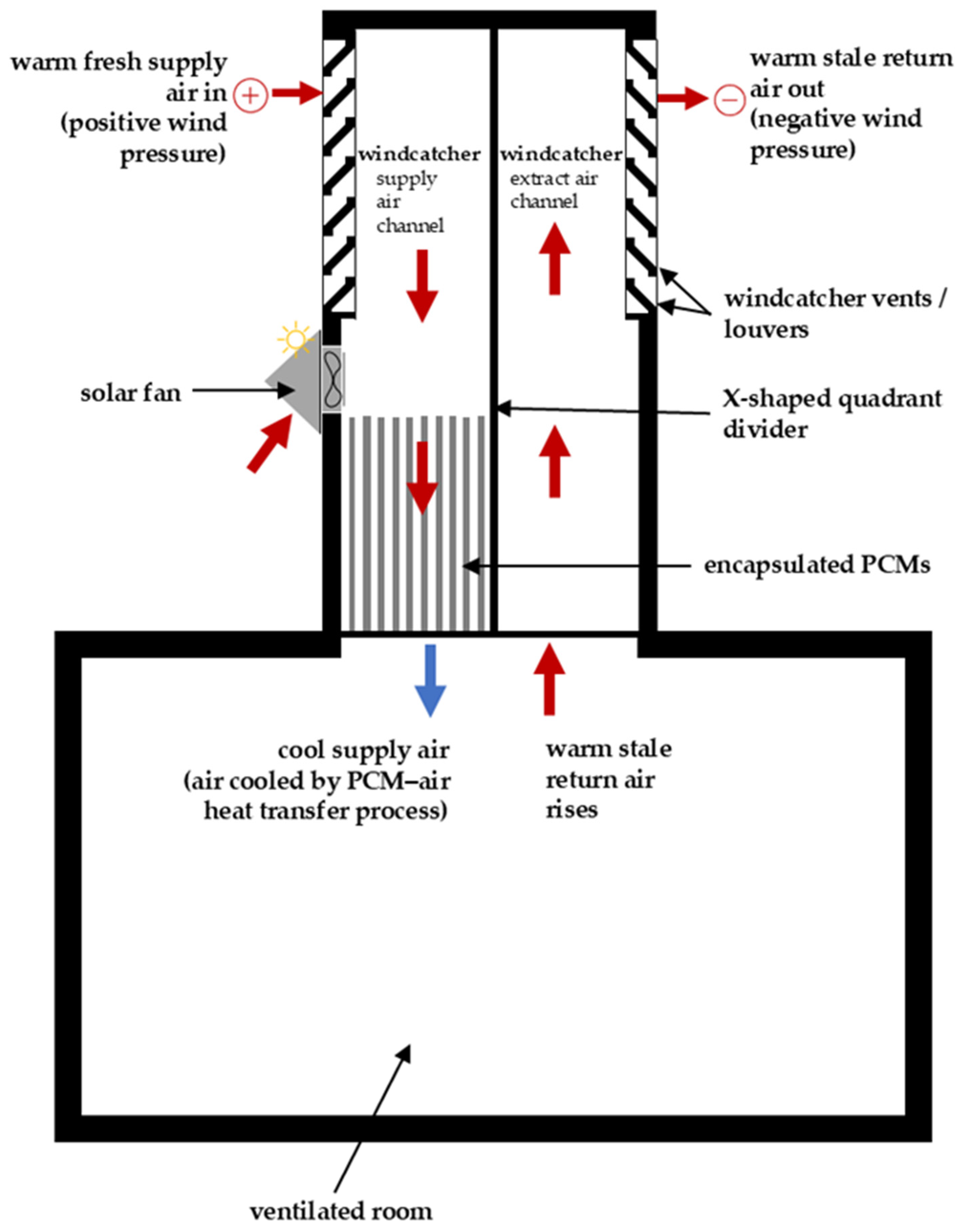
2.1. Proposed System
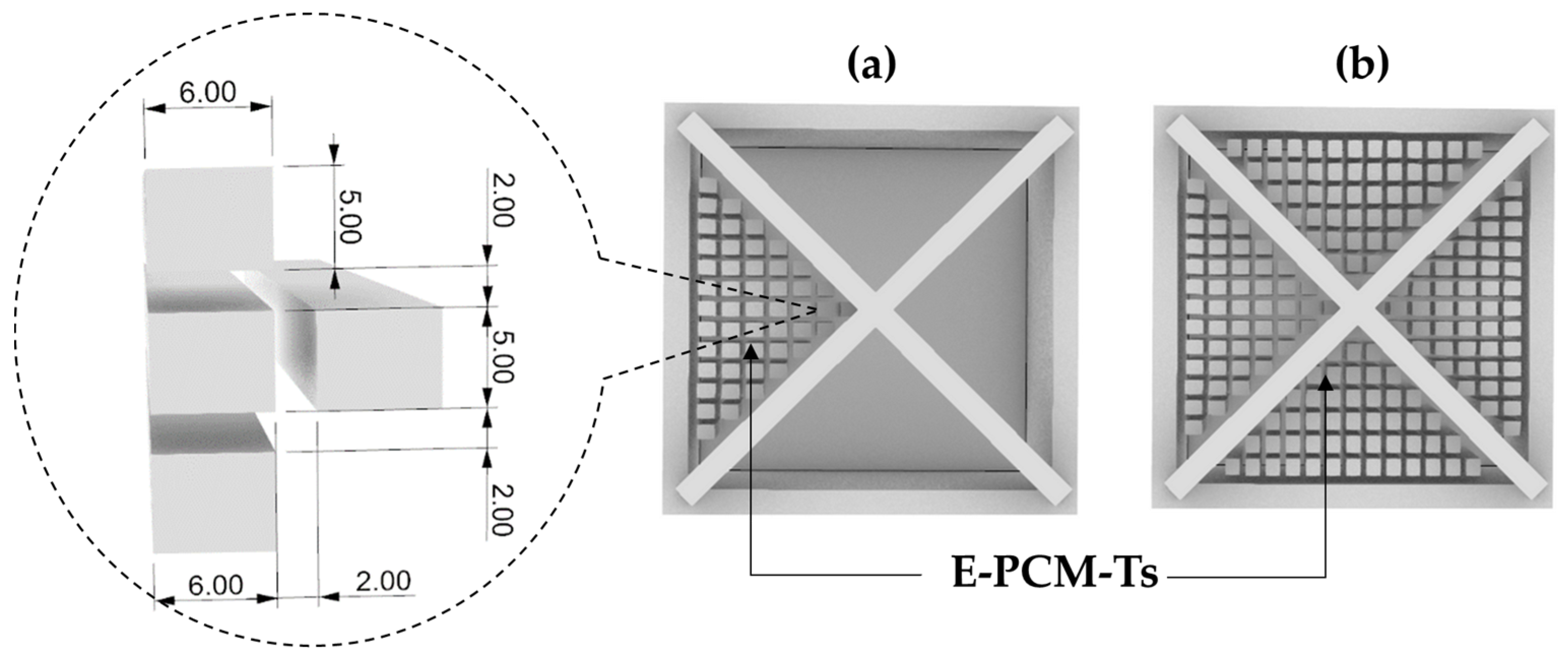
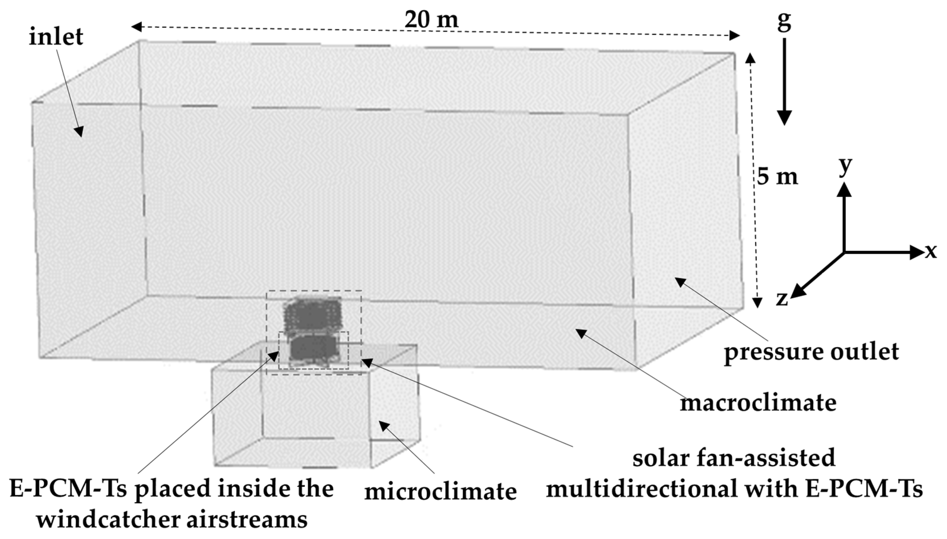
2.2. Geometry and Computational Domain
2.3. Material Selection
2.4. CFD Numerical Modeling
2.4.1. Assumptions
- The initial temperature of the PCM was set at 293 K (20 °C).
- Volume expansion of the PCM during phase change was neglected in the solution computation.
- The PCM was considered isotropic, with uniform thermal conductivity.
- All thermophysical properties were assumed to be homogenous and constant, independent of temperature variations.
- Convective heat loss around the windcatcher and room walls was neglected, assuming adiabatic conditions.
- Airflow in the model was assumed to be incompressible, transient, and turbulent.
2.4.2. Governing Equations
Governing Equations for the Airflow Within the Model
Governing Equations for the PCM Phase Transition Heat Transfer Interfaces
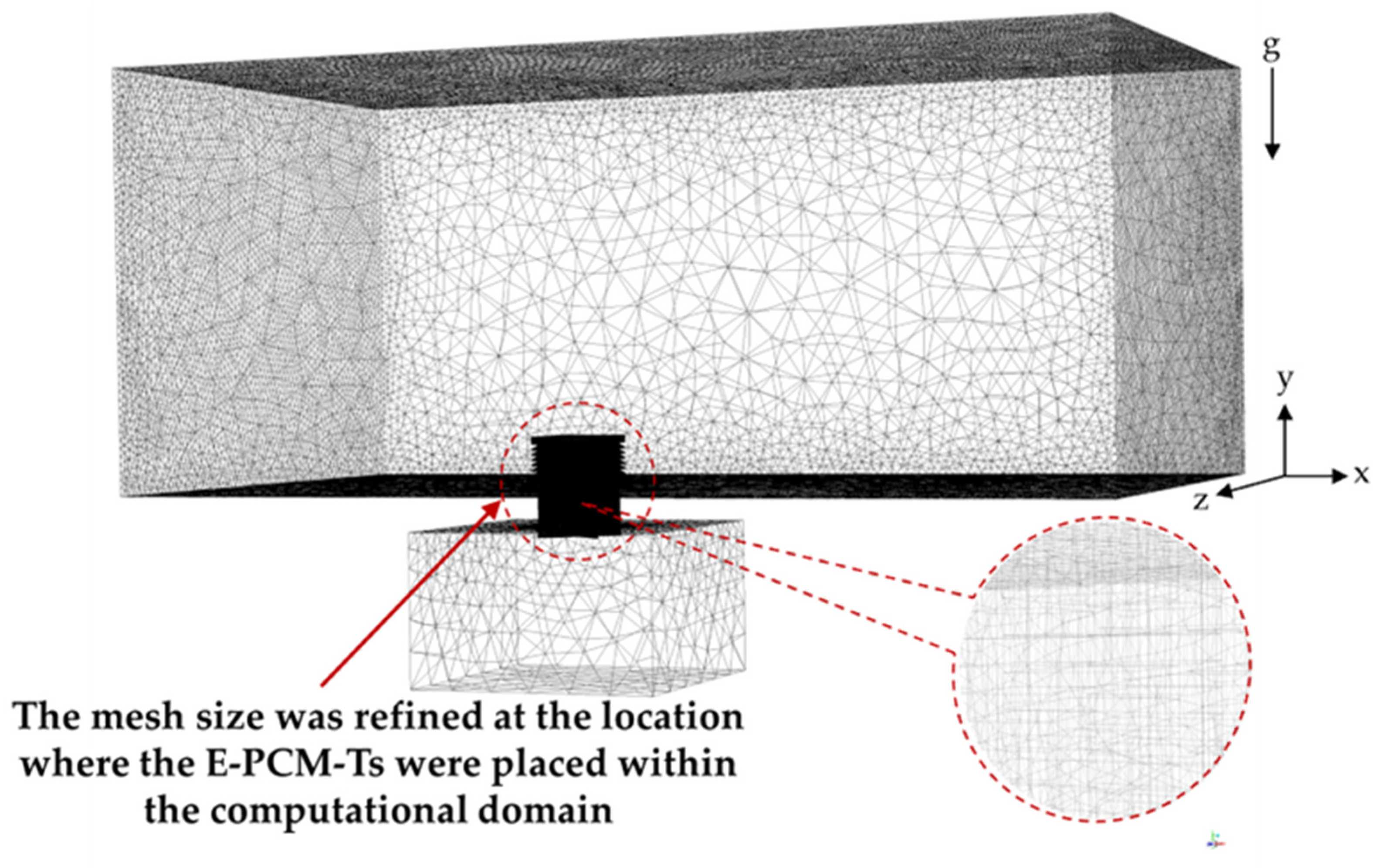
2.4.3. Mesh Generation and Adaptation
2.4.4. Grid Sensitivity Analysis
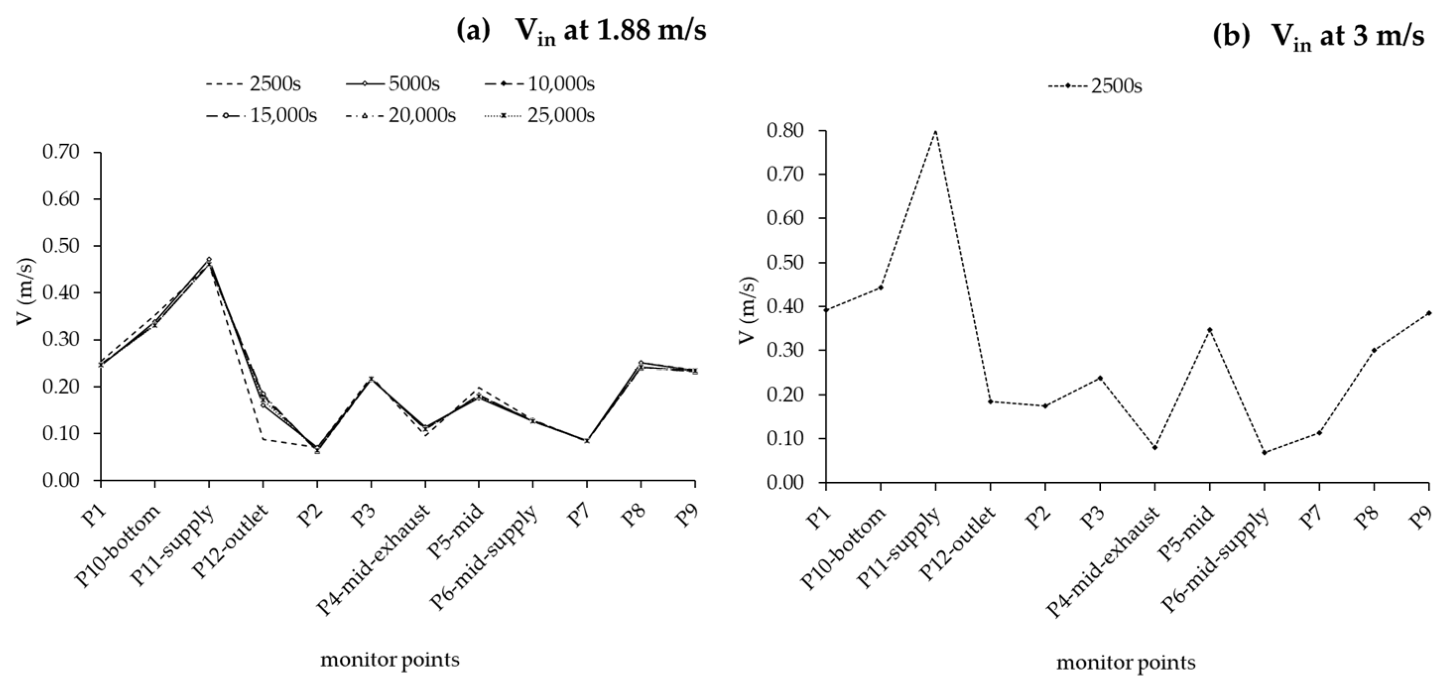
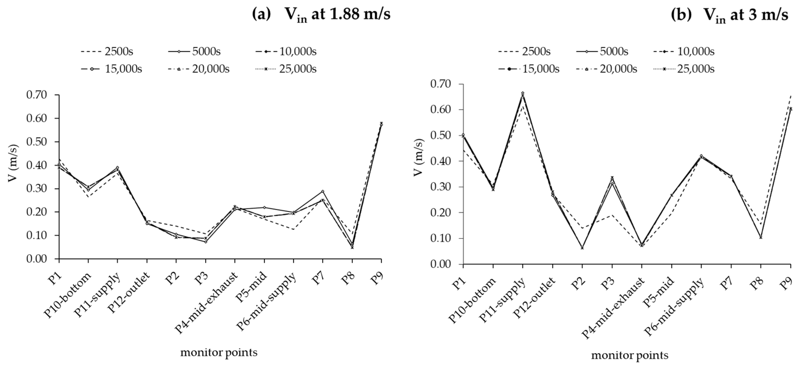
2.4.5. Timestep Independence Study
2.4.6. Boundary Conditions
2.4.7. Solution Convergence
3. Validation of Numerical Method
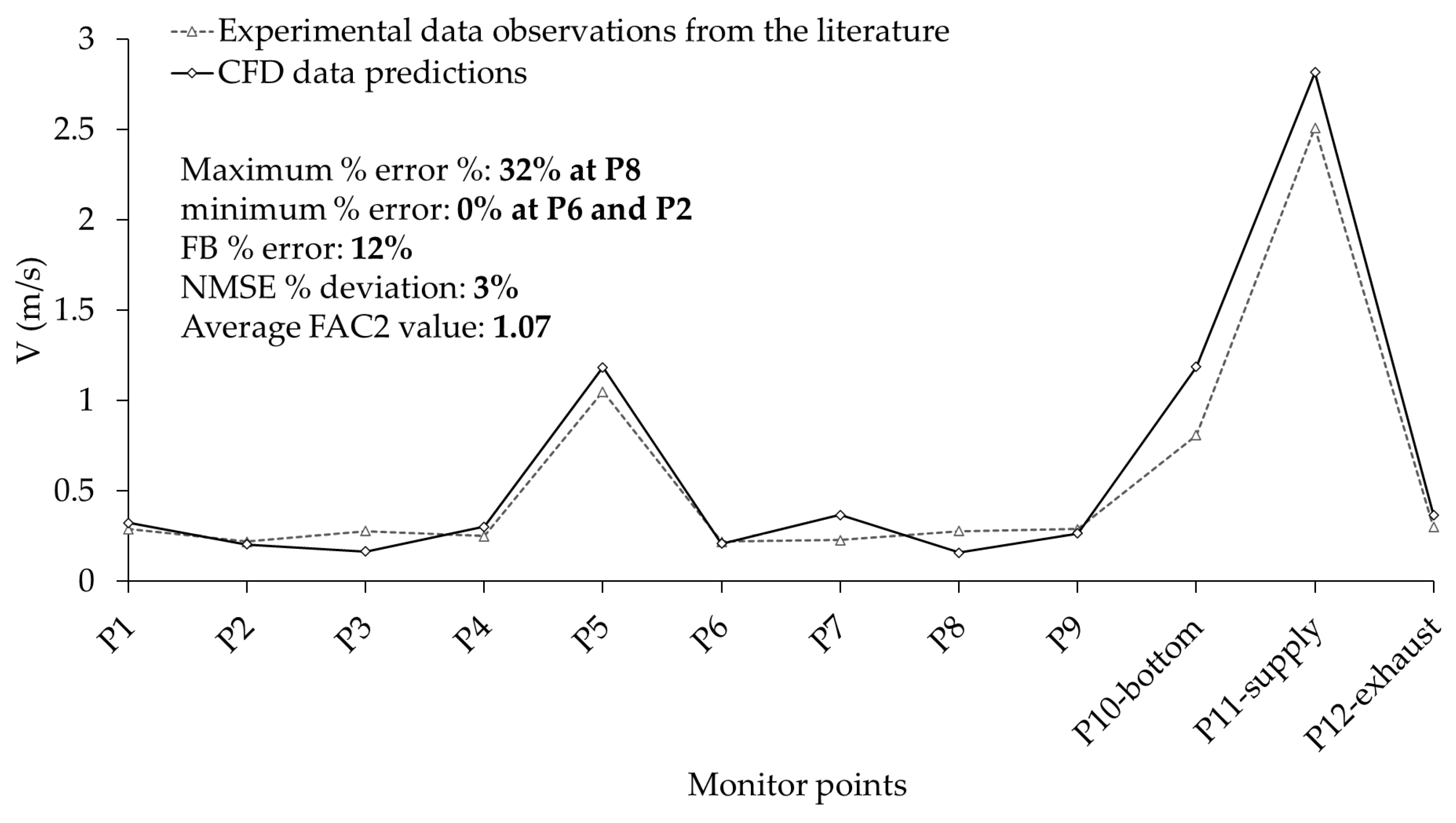
3.1. Windcatcher Airflow Model Validation
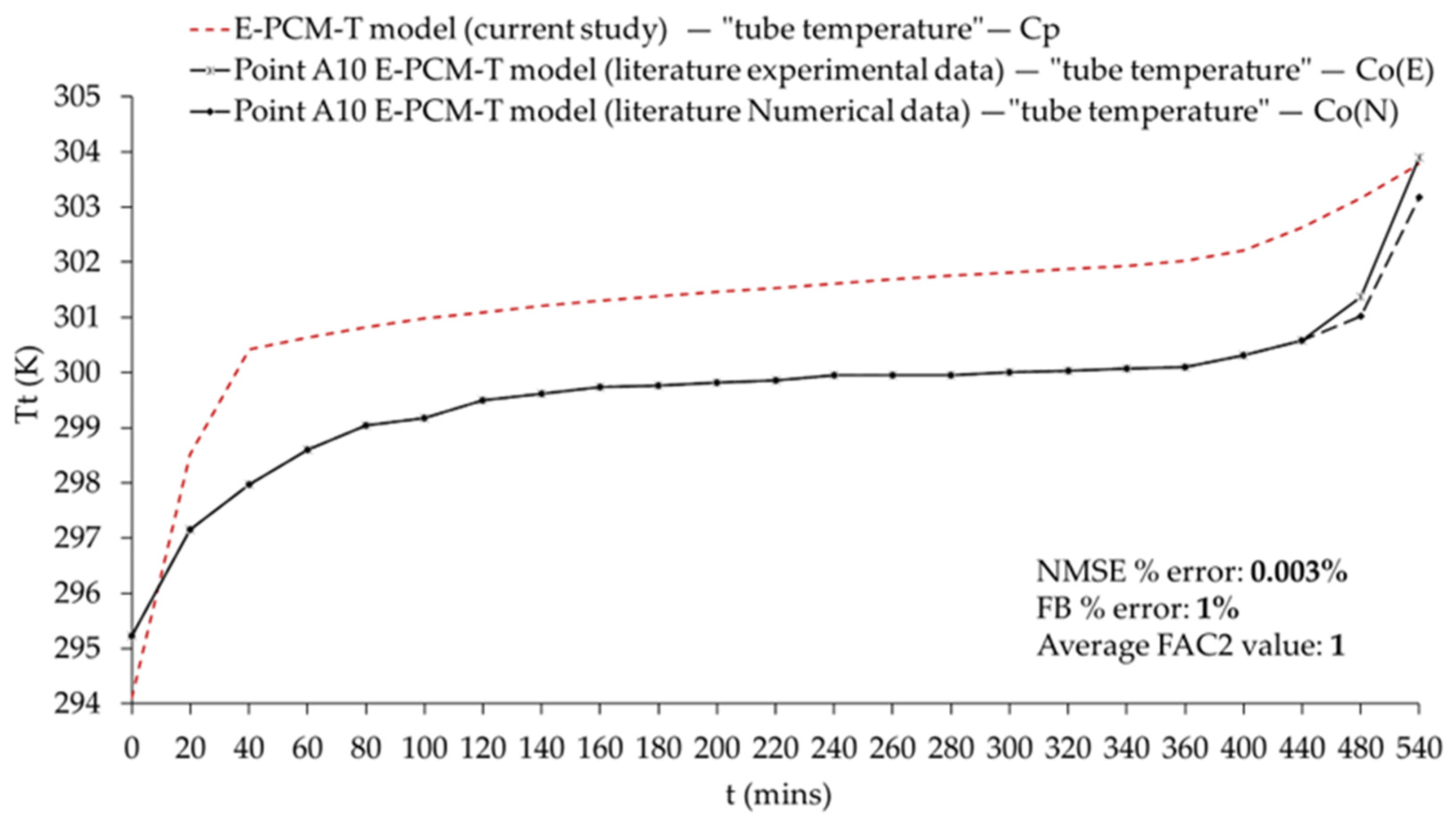
3.2. E-PCM-T Liquid Fraction Model Validation
4. Results and Discussion
4.1. Ventilation Performance Assessment
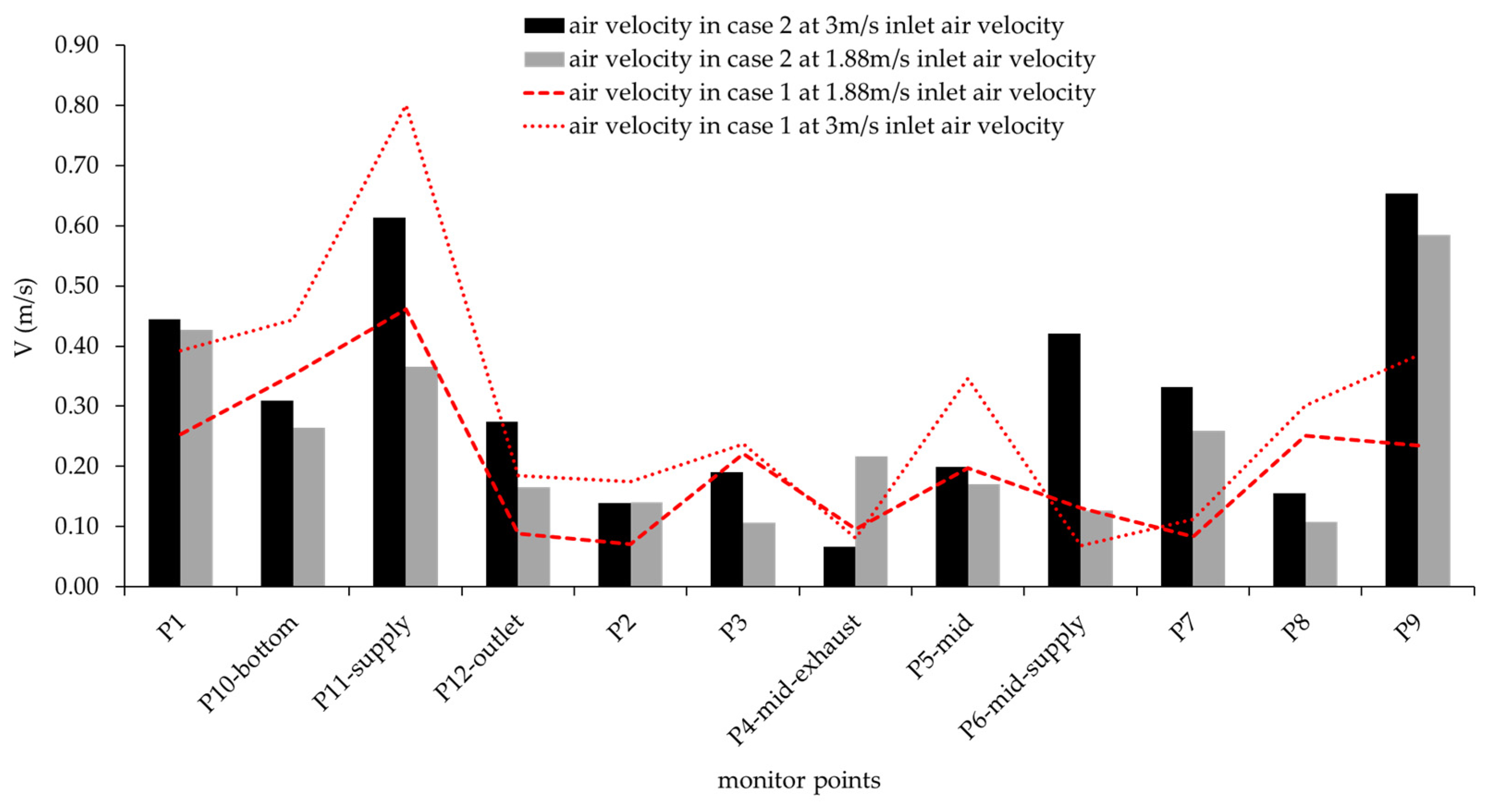
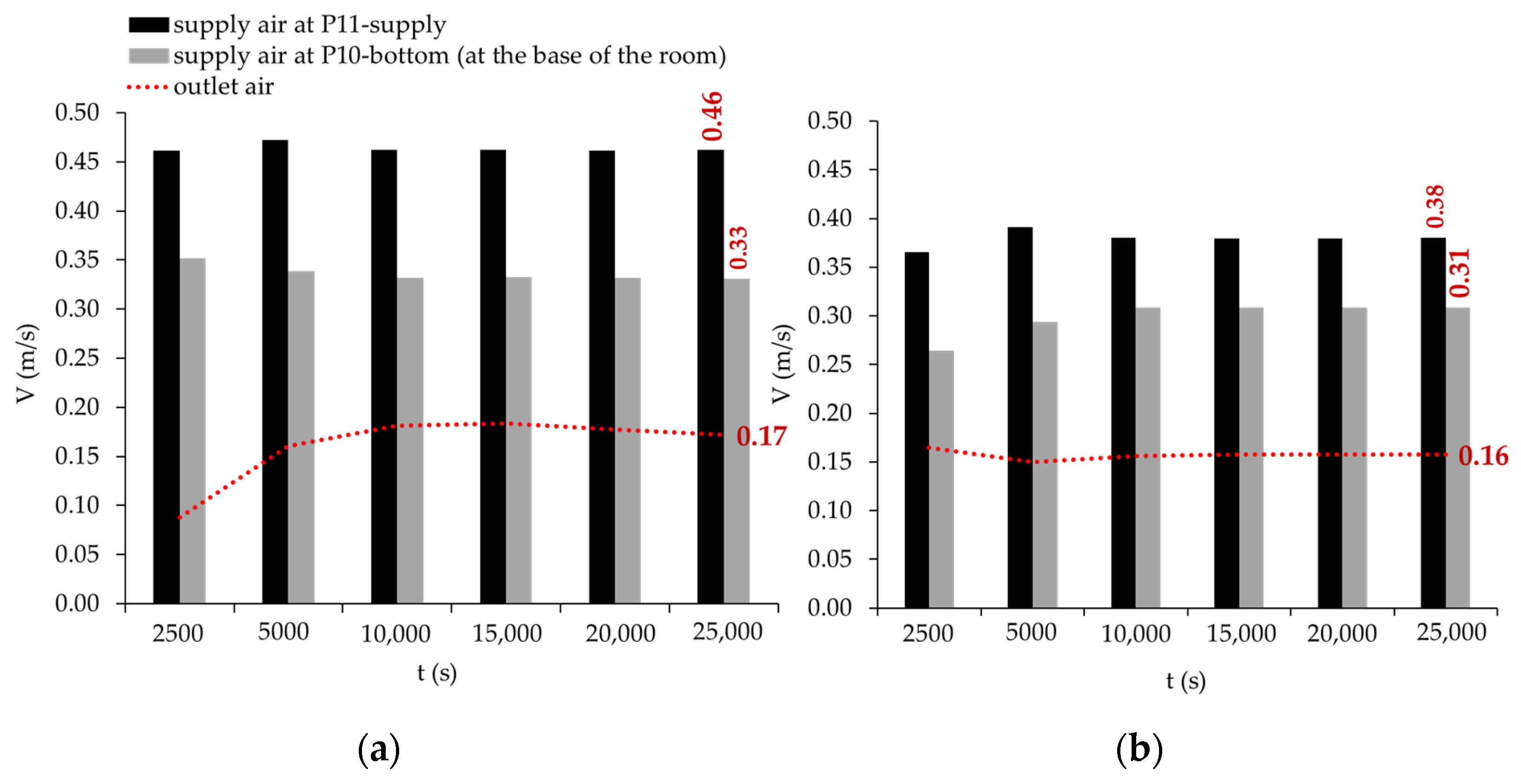
4.1.1. Impact of Varying Outdoor Wind Speeds on Ventilation Performance
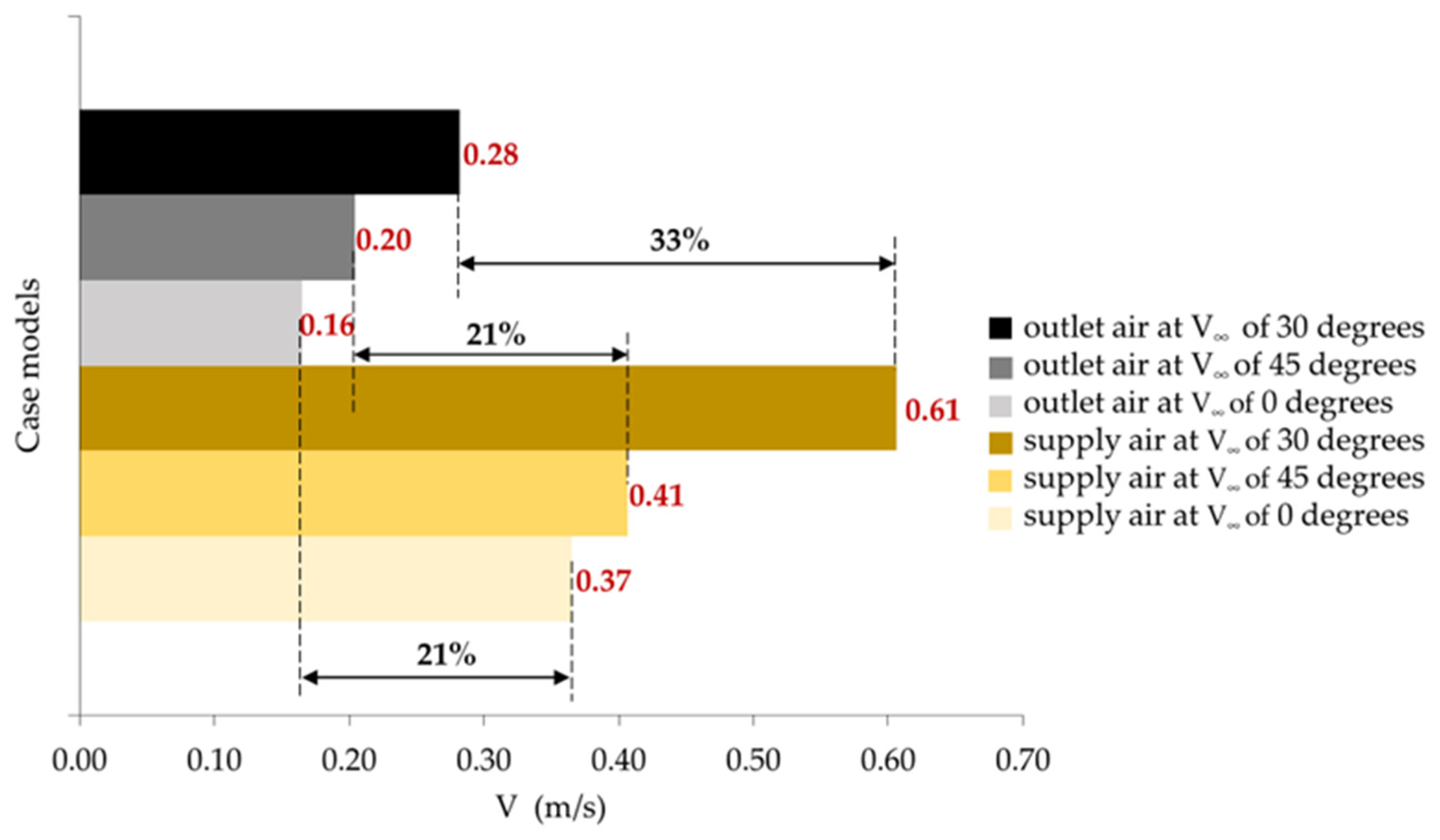
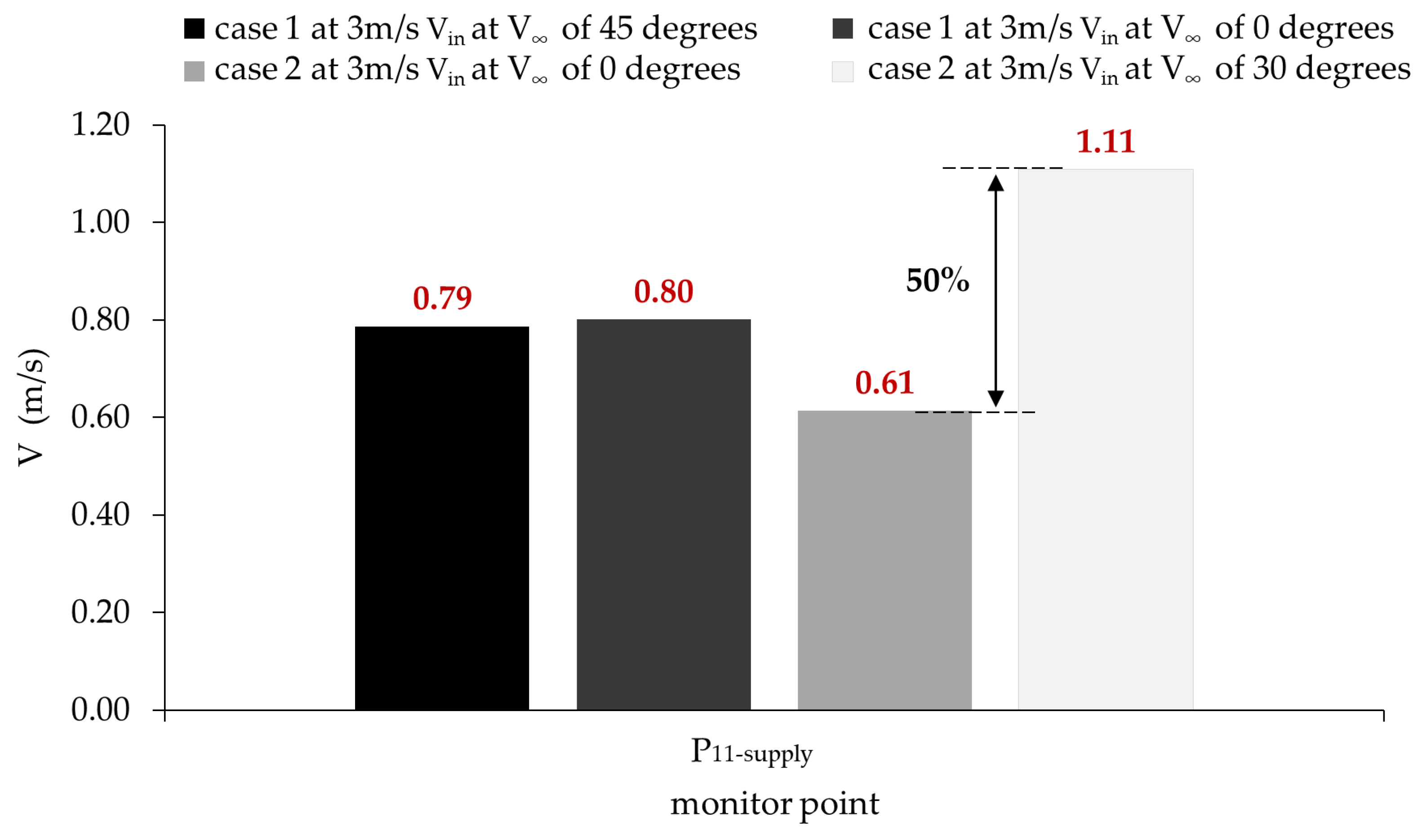
4.1.2. Impact of Varying Outdoor Wind Angles on Ventilation Performance
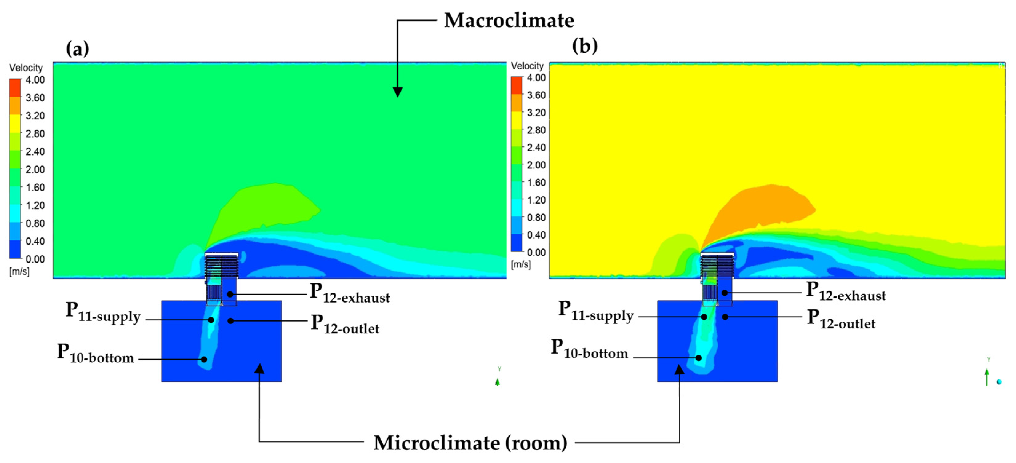
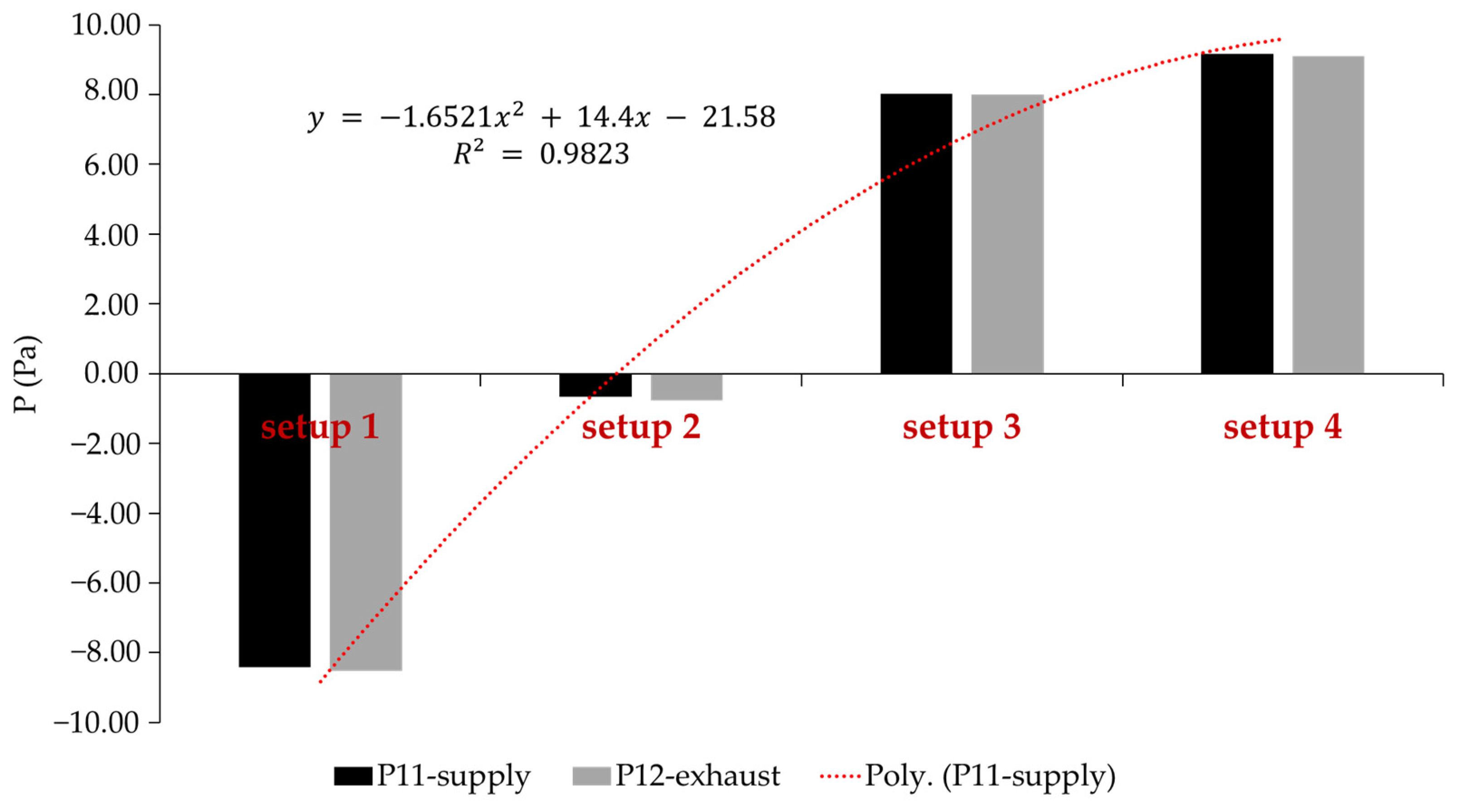
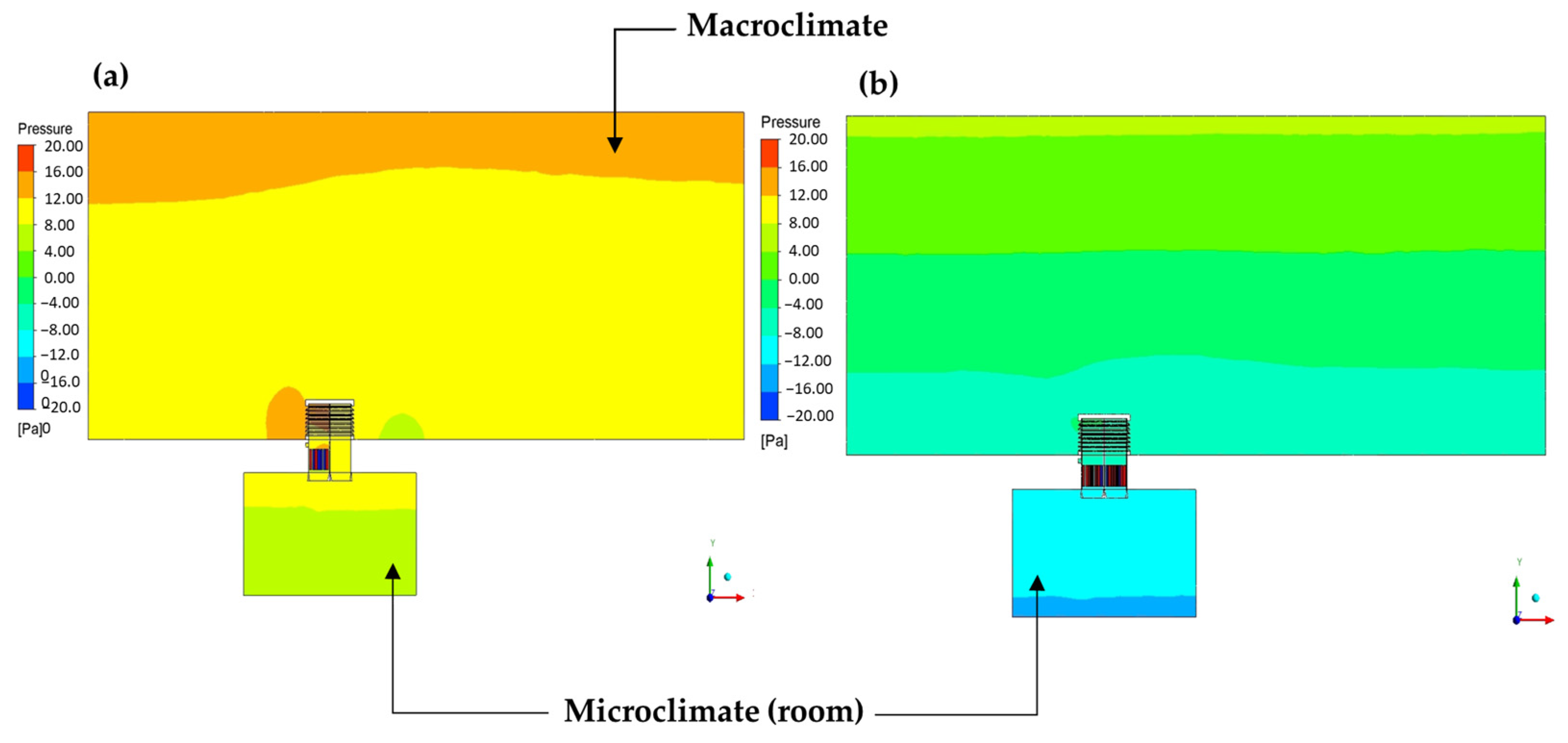
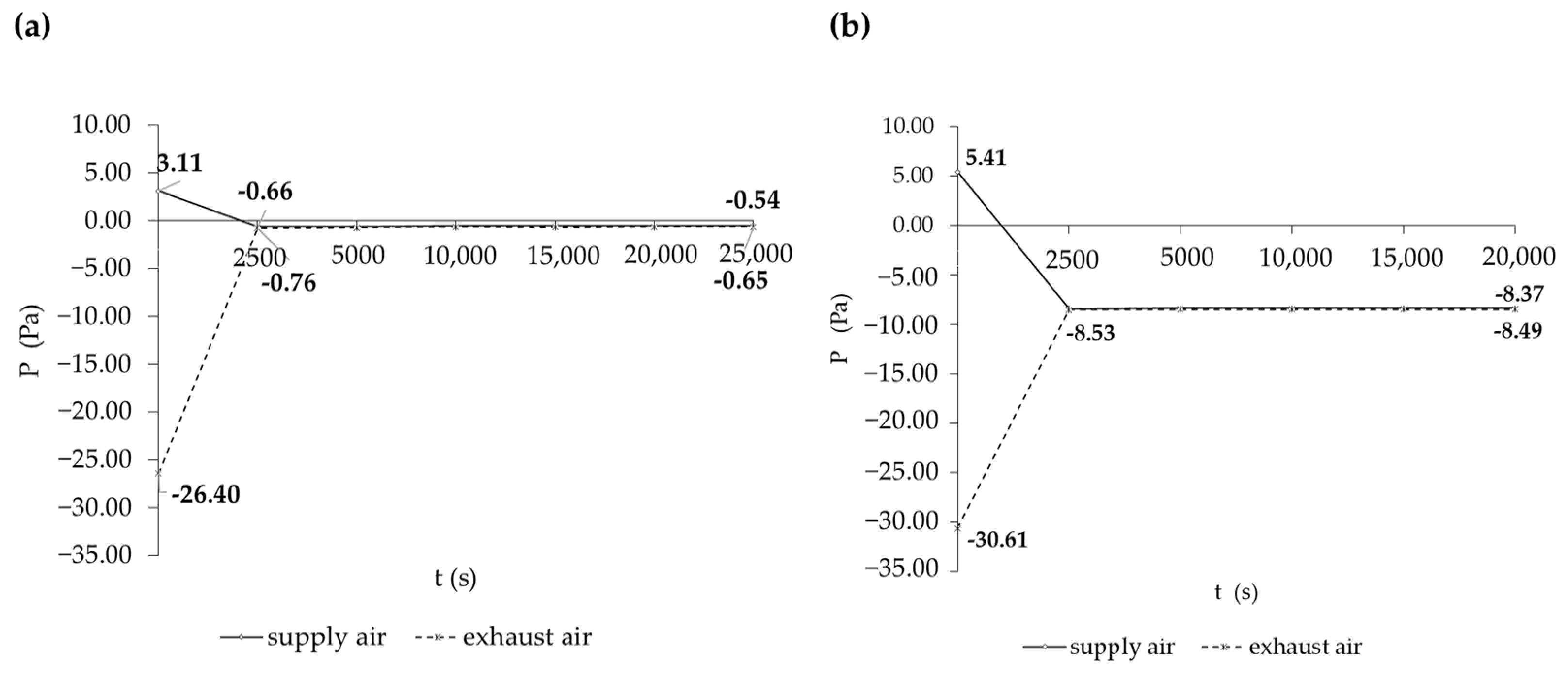
4.1.3. Air Pressure Distribution in the Model
4.2. Cooling Performance Assessment
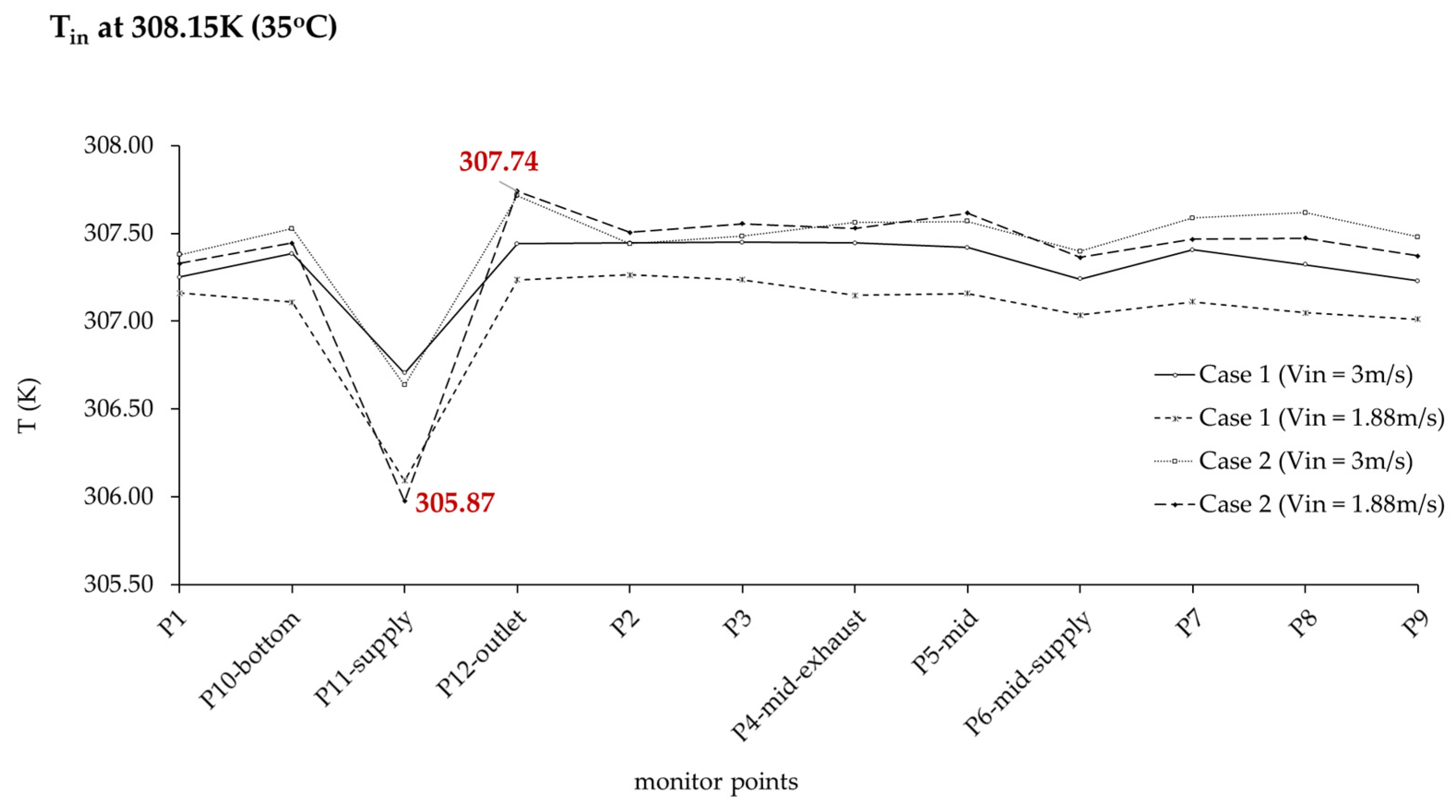
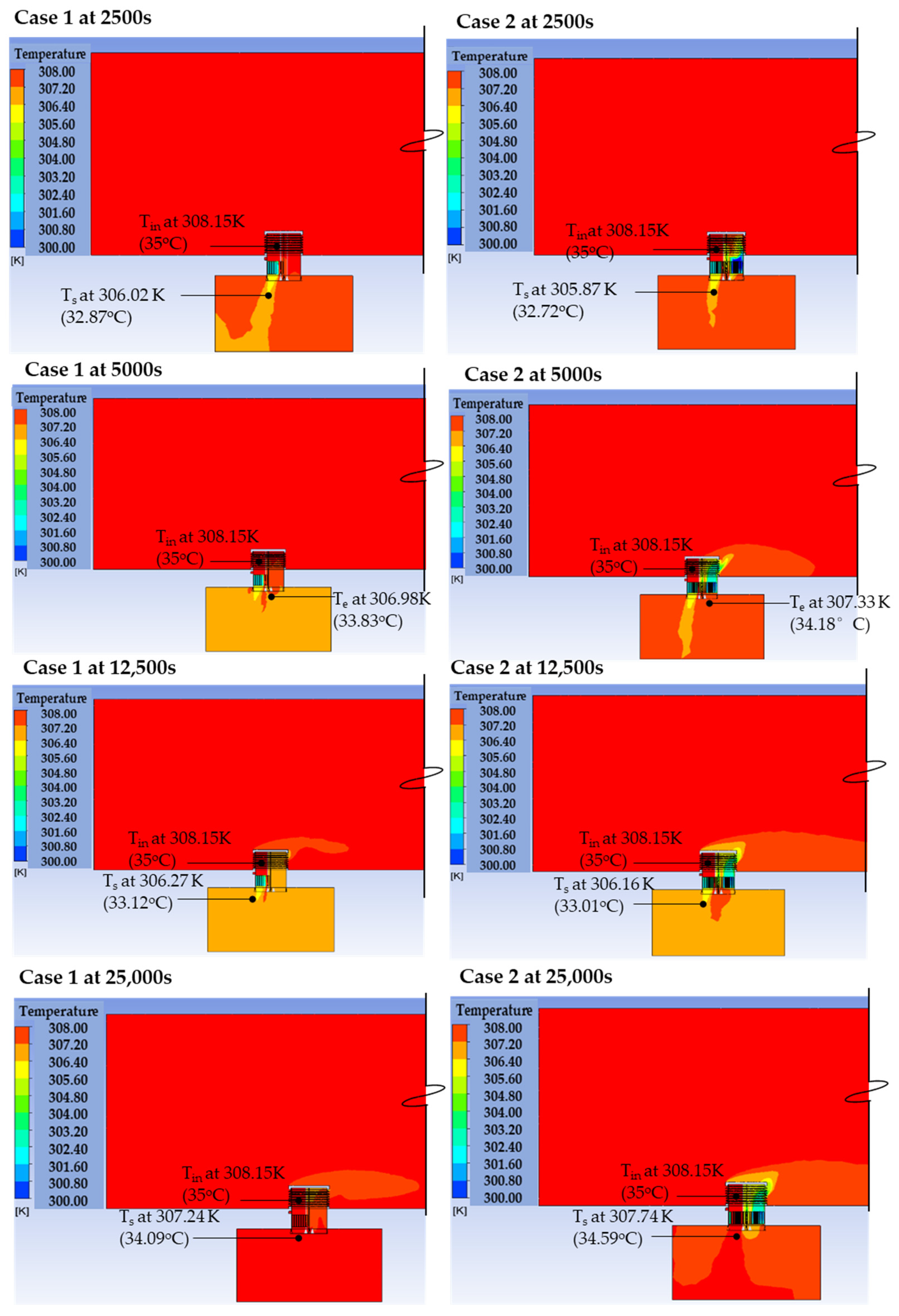
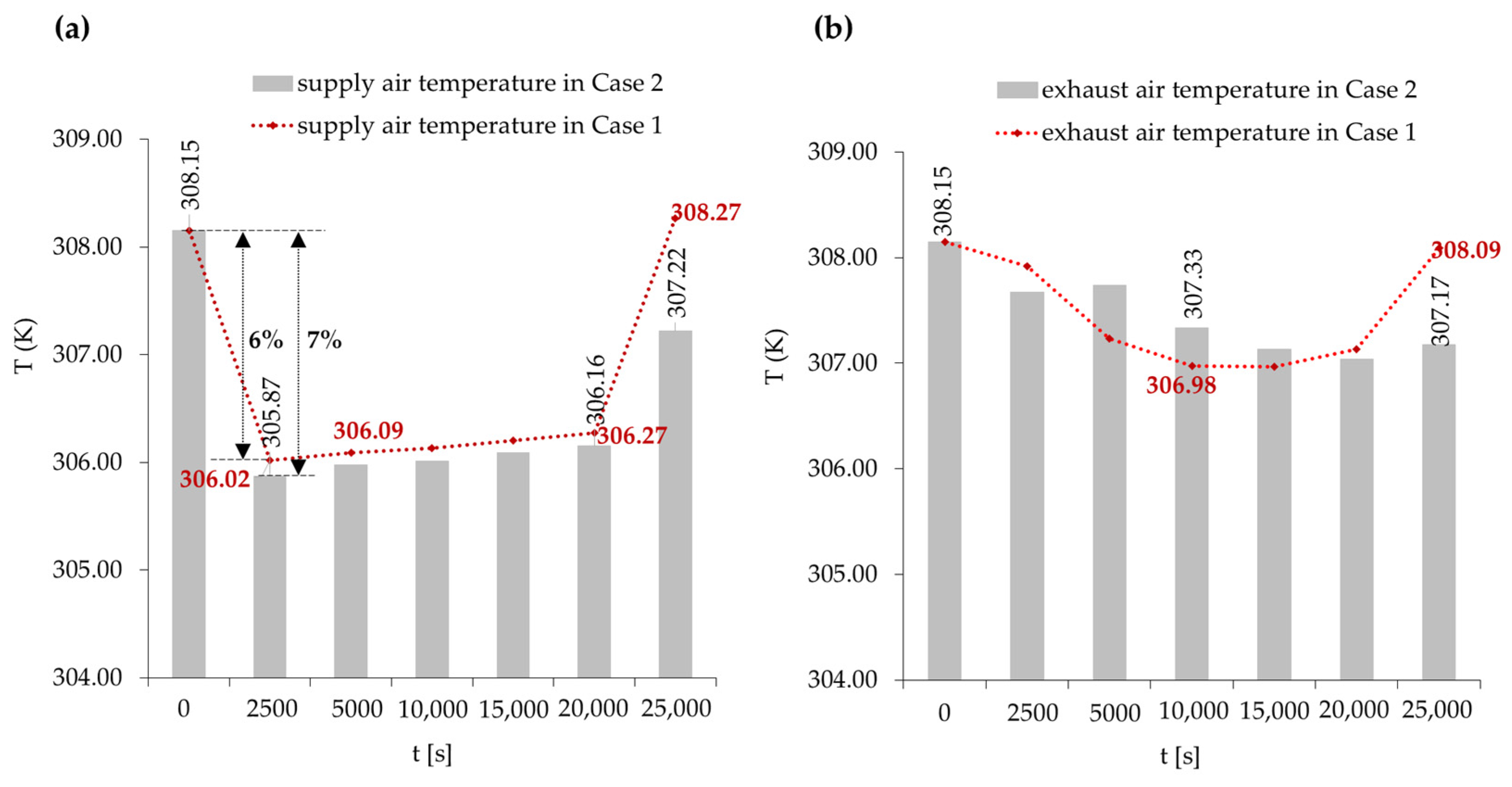
4.2.1. The Impact of Varying Outdoor Wind Speeds on Cooling Performance
4.2.2. Impact of E-PCMT Arrangement on Cooling Performance
4.3. Thermal Energy Storage Performance Assessment
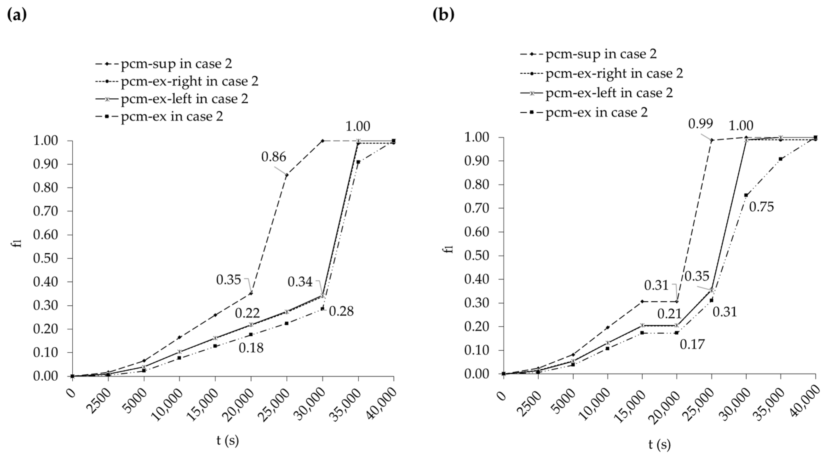
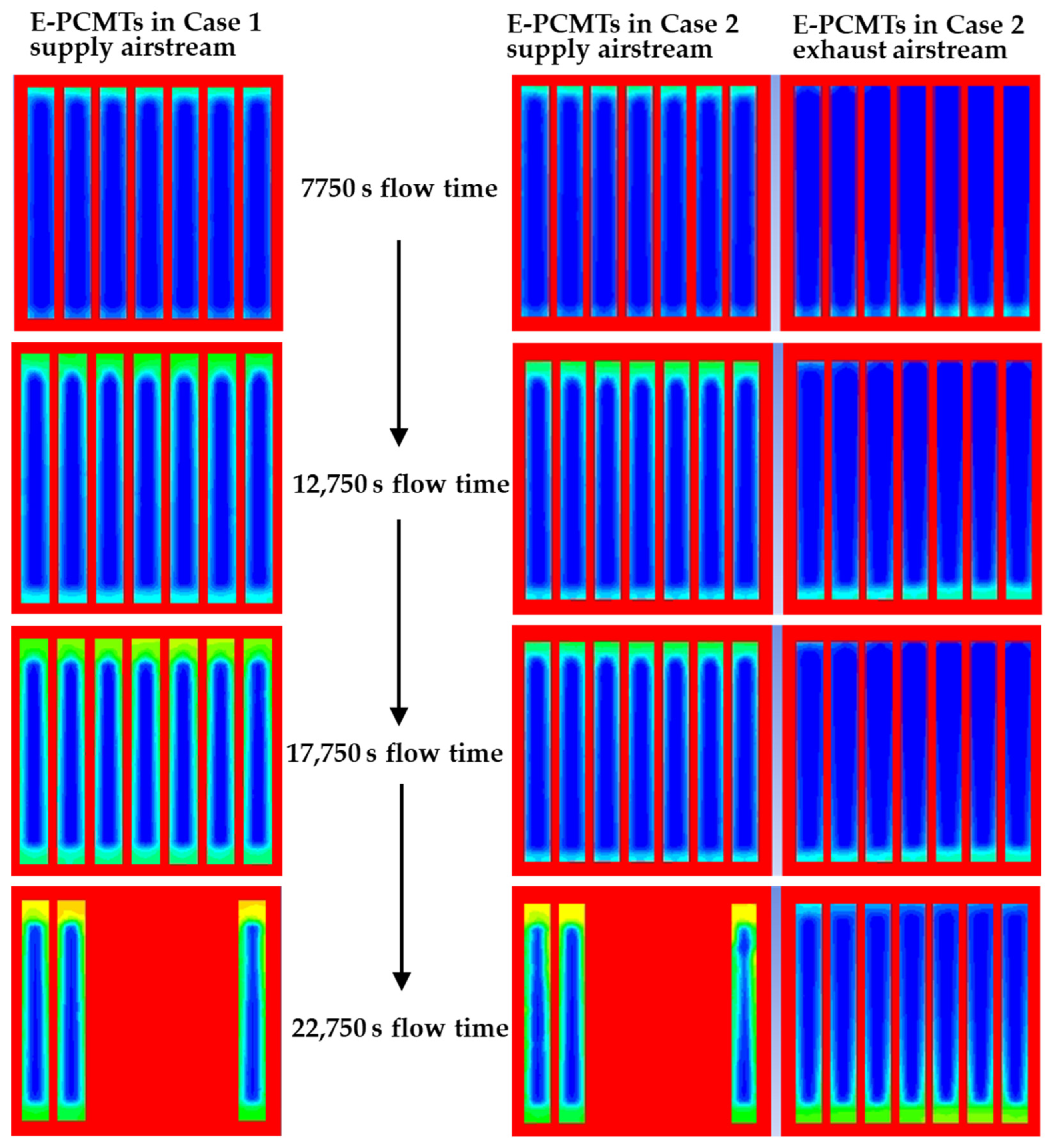
4.3.1. Impact of Varying Outdoor Wind Speeds on Thermal Energy Storage Performance
4.3.2. Impact of E-PCMT Arrangement on Thermal Storage Performance
5. Conclusions
5.1. Ventilation Performance
5.2. Cooling Performance
5.3. Thermal Energy Storage
5.4. Future Research
Author Contributions
Funding
Data Availability Statement
Acknowledgments
Conflicts of Interest
Nomenclature
| absorbed heat in a room per unit area surface. | |
| air temperature | |
| V | air velocity |
| daytime room temperature | |
| density of air | |
| effective heat conductivity | |
| Te | exhaust air temperature |
| Ve | exhaust air velocity |
| data set average | |
| CFD model predictions | |
| empirical model constant | |
| empirical model constant | |
| empirical model constant | |
| experiment observations | |
| Pe | exhaust air pressure |
| fluid-specific enthalpy | |
| fluid velocity in the model | |
| fusion flux of species | |
| gravitational acceleration | |
| Tin | inlet air temperature |
| V∞ | inlet wind angle |
| Vin | inlet wind speed |
| inner tube dimeter | |
| mass flux | |
| molecular dynamic viscosity | |
| net rate of production of species | |
| nighttime room temperature | |
| optimal PCM melting temperature | |
| Tout | outdoor temperature |
| outer tube diameter | |
| PCM charging time | |
| PCM density | |
| PCM discharging time | |
| PCM liquid fraction | |
| PCM mass | |
| Tpcm | PCM temperature |
| ΔTpcm | PCM temperature difference |
| PCM temperature at solid | |
| PCM volume fraction | |
| PCM volume | |
| D% | percentage deviation at every data point |
| P | point |
| air pressure | |
| rate of creating species by addition | |
| s | seconds |
| set average room temperature | |
| S | simulation coefficient |
| species | |
| specific internal energy | |
| Ps | supply air pressure |
| Ts | supply air temperature |
| Vs | supply air velocity |
| ΔT | temperature difference |
| thermal expansion coefficient | |
| time | |
| TKE source caused by average velocity gradient | |
| TKE source based on buoyancy force | |
| Tt | tube temperature |
| tube length | |
| tube height | |
| tube width | |
| turbulent Prandtl constant | |
| turbulent Prandtl constant | |
| turbulence stress divergence due to the velocity fluctuations by the auxiliary stresses | |
| Glossary | |
| AC | Air conditioning |
| Case 1 | Windcatcher model assisted by solar fan with E-PCM-Ts included in only supply airstream |
| Case 2 | Windcatcher model assisted by solar fan with E-PCM-Ts included in all four airstreams |
| CFD | Computational fluid dynamics |
| E-PCM-T | Encapsulated phase-change material tubes |
| GHG | Global greenhouse gas |
| HVAC | Heating, ventilation, and air conditioning |
| PCM | Phase-change material |
References
- Li, Y.; Han, M.; Liu, S.; Chen, G. Energy consumption and greenhouse gas emissions by buildings: A multi-scale perspective. Build. Environ. 2019, 151, 240–250. [Google Scholar] [CrossRef]
- Jafari, S.; Kalantar, V. Numerical simulation of natural ventilation with passive cooling by diagonal solar chimneys and windcatcher and water spray system in a hot and dry climate. Energy Build. 2022, 256, 111714. [Google Scholar] [CrossRef]
- Zhong, F.; Calautit, J.K.; Wu, Y. Assessment of HVAC system operational fault impacts and multiple faults interactions under climate change. Energy 2022, 258, 124762. [Google Scholar] [CrossRef]
- Uddin, K.; Saha, B.B. An Overview of Environment-Friendly Refrigerants for Domestic Air Conditioning Applications. Energies 2022, 15, 8082. [Google Scholar] [CrossRef]
- Dong, Y.; Coleman, M.; Miller, S.A. Greenhouse Gas Emissions from Air Conditioning and Refrigeration Service Expansion in Developing Countries. Annu. Rev. Environ. Resour. 2021, 46, 59–83. [Google Scholar] [CrossRef]
- Woods, J.; James, N.; Kozubal, E.; Bonnema, E.; Brief, K.; Voeller, L.; Rivest, J. Humidity’s impact on greenhouse gas emissions from air conditioning. Joule 2022, 6, 726–741. [Google Scholar] [CrossRef]
- Calautit, J.K.; O’connor, D.; Tien, P.W.; Wei, S.; Pantua, C.A.J.; Hughes, B. Development of a natural ventilation windcatcher with passive heat recovery wheel for mild-cold climates: CFD and experimental analysis. Renew. Energy 2020, 160, 465–482. [Google Scholar] [CrossRef]
- Rashid, S.A.; Haider, Z.; Hossain, S.M.C.; Memon, K.; Panhwar, F.; Mbogba, M.K.; Hu, P.; Zhao, G. Retrofitting low-cost heating ventilation and air-conditioning systems for energy management in buildings. Appl. Energy 2019, 236, 648–661. [Google Scholar] [CrossRef]
- Nejat, P.; Calautit, J.K.; Fekri, Y.; Sheikhshahrokhdehkordi, M.; Alsaad, H.; Voelker, C. Influence of terrain and atmospheric boundary layer on the ventilation and thermal comfort performance of windcatchers. J. Build. Eng. 2023, 73, 106791. [Google Scholar] [CrossRef]
- Kim, M.K.; Barber, C.; Srebric, J. Traffic noise level predictions for buildings with windows opened for natural ventilation in urban environments. Sci. Technol. Built Environ. 2017, 23, 726–735. [Google Scholar] [CrossRef]
- Prima, Y.; Prima, S. Wind Catcher and Solar Chimney Integrated As An Alternative Ventilation For Urban Dense Settlements In Tropical Climate. Int. J. Arch. Urban. 2019, 3, 51–68. [Google Scholar] [CrossRef]
- Nejat, P.; Jomehzadeh, F. Windcatcher as a Persian sustainable solution for passive cooling. Civ. Eng. Res. J. 2018, 6, 7. [Google Scholar] [CrossRef]
- Bahadori, M.N.; Dehghani-Sanij, A.; Sayigh, A. Wind Towers; Springer: Berlin/Heidelberg, Germany, 2016. [Google Scholar]
- Arias-Jiménez, N.; Trebilcock-Kelly, M.; Moreno, A.B.; San-Martín, R.F. Wind towers: Potential evaluation of natural ventilation in housing. Arquiteturarevista 2021, 17, 198–218. [Google Scholar] [CrossRef]
- Yazarlou, T.; Barzkar, E. Louver and window position effect on cross-ventilation in a generic isolated building: A CFD approach. Indoor Built Environ. 2019, 31, 1511–1529. [Google Scholar] [CrossRef]
- Li, L.; Mak, C. The assessment of the performance of a windcatcher system using computational fluid dynamics. Build. Environ. 2007, 42, 1135–1141. [Google Scholar] [CrossRef]
- Sangdeh, P.K.; Nasrollahi, N. Windcatchers and their applications in contemporary architecture. Energy Built Environ. 2022, 3, 56–72. [Google Scholar] [CrossRef]
- Pelletier, K.; Calautit, J. Analysis of the performance of an integrated multistage helical coil heat transfer device and passive cooling windcatcher for buildings in hot climates. J. Build. Eng. 2022, 48, 103899. [Google Scholar] [CrossRef]
- Chen, Q. Ventilation performance prediction for buildings: A method overview and recent applications. Build. Environ. 2009, 44, 848–858. [Google Scholar] [CrossRef]
- Li, J.; Calautit, J.K.; Jimenez-Bescos, C. Experiment and numerical investigation of a novel flap fin louver windcatcher for multi-directional natural ventilation and passive technology integration. Build. Environ. 2023, 242, 110429. [Google Scholar] [CrossRef]
- Li, J.; Calautit, J.; Jimenez-Bescos, C. Parametric analysis of a novel rotary scoop dual-channel windcatcher for multi-directional natural ventilation of buildings. Energy Built Environ. 2024; in press. [Google Scholar] [CrossRef]
- Nejat, P.; Fekri, Y.; Sheikhshahrokhdehkordi, M.; Jomehzadeh, F.; Alsaad, H.; Voelker, C. The Windcatcher: A Renewable-Energy-Powered Device for Natural Ventilation—The Impact of Upper Wing Walls. Energies 2024, 17, 611. [Google Scholar] [CrossRef]
- Yang, Y.K.; Kim, M.Y.; Song, Y.W.; Choi, S.H.; Park, J.C. Windcatcher louvers to improve ventilation efficiency. Energies 2020, 13, 4459. [Google Scholar] [CrossRef]
- Zaki, A.; Richards, P.; Sharma, R. The effect of onset turbulent flows on ventilation with a two-sided rooftop windcatcher. J. Wind. Eng. Ind. Aerodyn. 2022, 225, 104993. [Google Scholar] [CrossRef]
- Khakzand, M.; Deljouiee, B.; Chahardoli, S.; Siavashi, M. Radiative cooling ventilation improvement using an integrated system of windcatcher and solar chimney. J. Build. Eng. 2024, 83, 108409. [Google Scholar] [CrossRef]
- Li, J.; Calautit, J.; Jimenez-Bescos, C.; Riffat, S. Experimental and numerical evaluation of a novel dual-channel windcatcher with a rotary scoop for energy-saving technology integration. Build. Environ. 2023, 230, 110018. [Google Scholar] [CrossRef]
- Shayegani, A.; Joklova, V.; Illes, J. Optimizing Windcatcher Designs for Effective Passive Cooling Strategies in Vienna’s Urban Environment. Buildings 2024, 14, 765. [Google Scholar] [CrossRef]
- Pakari, A.; Ghani, S. Airflow assessment in a naturally ventilated greenhouse equipped with wind towers: Numerical simulation and wind tunnel experiments. Energy Build. 2019, 199, 1–11. [Google Scholar] [CrossRef]
- Gharakhani, A.; Sediadi, E.; Roshan, M.; Sabzevar, H.B. Experimental study on performance of wind catcher in tropical climate. ARPN J. Eng. Appl. Sci. 2017, 12, 2551–2555. [Google Scholar]
- Calautit, J.K.; Hughes, B.R.; Shahzad, S.S. CFD and wind tunnel study of the performance of a uni-directional wind catcher with heat transfer devices. Renew. Energy 2015, 83, 85–99. [Google Scholar] [CrossRef]
- O’connor, D.; Calautit, J.K.; Hughes, B.R. A novel design of a desiccant rotary wheel for passive ventilation applications. Appl. Energy 2016, 179, 99–109. [Google Scholar] [CrossRef]
- Chohan, A.H.; Awad, J. Wind Catchers: An Element of Passive Ventilation in Hot, Arid and Humid Regions, a Comparative Analysis of Their Design and Function. Sustainability 2022, 14, 11088. [Google Scholar] [CrossRef]
- Dehghani-Sanij, A.; Soltani, M.; Raahemifar, K. A new design of wind tower for passive ventilation in buildings to reduce energy consumption in windy regions. Renew. Sustain. Energy Rev. 2015, 42, 182–195. [Google Scholar] [CrossRef]
- Zhang, B.; Hu, H.; Kikumoto, H.; Ooka, R. Turbulence-induced ventilation of an isolated building: Ventilation route identification using spectral proper orthogonal decomposition. Build. Environ. 2022, 223, 109471. [Google Scholar] [CrossRef]
- Jafari, D.; Shateri, A.; Nadooshan, A.A. Experimental and numerical study of natural ventilation in four-sided wind tower traps. Energy Equip. Syst. 2018, 6, 167–179. [Google Scholar]
- Afshin, M.; Sohankar, A.; Manshadi, M.D.; Esfeh, M.K. An experimental study on the evaluation of natural ventilation performance of a two-sided wind-catcher for various wind angles. Renew. Energy 2016, 85, 1068–1078. [Google Scholar] [CrossRef]
- Calautit, J.K.; Hughes, B.R. Wind tunnel and CFD study of the natural ventilation performance of a commercial multi-directional wind tower. Build. Environ. 2014, 80, 71–83. [Google Scholar] [CrossRef]
- Duan, S.; Jing, C.; Long, E. Transient flows in displacement ventilation enhanced by solar chimney and fan. Energy Build. 2015, 103, 124–130. [Google Scholar] [CrossRef]
- Zhang, H.; Yang, D.; Tam, V.W.; Tao, Y.; Zhang, G.; Setunge, S.; Shi, L. A critical review of combined natural ventilation techniques in sustainable buildings. Renew. Sustain. Energy Rev. 2021, 141, 110795. [Google Scholar] [CrossRef]
- Hughes, B.R.; Calautit, J.K.; Ghani, S.A. The development of commercial wind towers for natural ventilation: A review. Appl. Energy 2012, 92, 606–627. [Google Scholar] [CrossRef]
- Elmualim, A.A. Failure of a control strategy for a hybrid air-conditioning and wind catchers/towers system at Bluewater shopping malls in Kent, UK. Facilities 2006, 24, 399–411. [Google Scholar] [CrossRef]
- Hughes, B.R.; Ghani, S.A. A numerical investigation into the feasibility of a passive-assisted natural ventilation stack device. Int. J. Sustain. Energy 2011, 30, 193–211. [Google Scholar] [CrossRef]
- Lavafpour, Y.; Surat, M. Passive low energy architecture in hot and dry climate. Aust. J. Basic Appl. Sci. 2011, 5, 757–765. [Google Scholar]
- Calautit, J.K.; Hughes, B.R.; Nasir, D.S. Climatic analysis of a passive cooling technology for the built environment in hot countries. Appl. Energy 2017, 186, 321–335. [Google Scholar] [CrossRef]
- Chaudhry, H.N.; Calautit, J.K.; Hughes, B.R. Computational analysis of a wind tower assisted passive cooling technology for the built environment. J. Build. Eng. 2015, 1, 63–71. [Google Scholar] [CrossRef]
- Bouchahm, Y.; Bourbia, F.; Belhamri, A. Performance analysis and improvement of the use of wind tower in hot dry climate. Renew. Energy 2011, 36, 898–906. [Google Scholar] [CrossRef]
- Calautit, J.K.; Chaudhry, H.N.; Hughes, B.R.; Ghani, S.A. Comparison between evaporative cooling and a heat pipe assisted thermal loop for a commercial wind tower in hot and dry climatic conditions. Appl. Energy 2013, 101, 740–755. [Google Scholar] [CrossRef]
- Calautit, J.K.; O’Connor, D.; Sofotasiou, P.; Hughes, B.R. CFD simulation and optimisation of a low energy ventilation and cooling system. Computation 2014, 3, 128–149. [Google Scholar] [CrossRef]
- Liu, L.; Hammami, N.; Trovalet, L.; Bigot, D.; Habas, J.-P.; Malet-Damour, B. Description of phase change materials (PCMs) used in buildings under various climates: A review. J. Energy Storage 2022, 56, 105760. [Google Scholar] [CrossRef]
- Yang, L.; Jin, X.; Zhang, Y.; Du, K. Recent development on heat transfer and various applications of phase-change materials. J. Clean. Prod. 2021, 287, 124432. [Google Scholar] [CrossRef]
- Al-Absi, Z.A.; Hafizal, M.I.M.; Ismail, M.; Mardiana, A.; Ghazali, A. Peak indoor air temperature reduction for buildings in hot-humid climate using phase change materials. Case Stud. Therm. Eng. 2020, 22, 100762. [Google Scholar] [CrossRef]
- O’connor, D.; Calautit, J.K.S.; Hughes, B.R. A review of heat recovery technology for passive ventilation applications. Renew. Sustain. Energy Rev. 2016, 54, 1481–1493. [Google Scholar] [CrossRef]
- Seidabadi, L.; Ghadamian, H.; Aminy, M. A Novel Integration of PCM with Wind-Catcher Skin Material in Order to Increase Heat Transfer Rate. Int. J. Renew. Energy Dev. 2019, 8, 1–6. [Google Scholar] [CrossRef]
- Lizana, J.; De-Borja-Torrejon, M.; Barrios-Padura, A.; Auer, T.; Chacartegui, R. Passive cooling through phase change materials in buildings. A critical study of implementation alternatives. Appl. Energy 2019, 254, 113658. [Google Scholar] [CrossRef]
- Rouault, F.; Bruneau, D.; Sebastian, P.; Lopez, J. Numerical modelling of tube bundle thermal energy storage for free-cooling of buildings. Appl. Energy 2013, 111, 1099–1106. [Google Scholar] [CrossRef]
- Abdo, P.; Huynh, B.P.; Braytee, A.; Taghipour, R. An experimental investigation of the thermal effect due to discharging of phase change material in a room fitted with a windcatcher. Sustain. Cities Soc. 2020, 61, 102277. [Google Scholar] [CrossRef]
- Calautit, J.K.; Aquino, A.I.; Shahzad, S.; Nasir, D.S.; Hughes, B.R. Thermal Comfort and Indoor air Quality Analysis of a Low-energy Cooling Windcatcher. Energy Procedia 2017, 105, 2865–2870. [Google Scholar] [CrossRef]
- Sharshir, S.W.; Joseph, A.; Elsharkawy, M.; Hamada, M.A.; Kandeal, A.; Elkadeem, M.R.; Thakur, A.K.; Ma, Y.; Moustapha, M.E.; Rashad, M.; et al. Thermal energy storage using phase change materials in building applications: A review of the recent development. Energy Build. 2023, 285, 112908. [Google Scholar] [CrossRef]
- Mosaffa, A.; Farshi, L.G.; Ferreira, C.I.; Rosen, M. Energy and exergy evaluation of a multiple-PCM thermal storage unit for free cooling applications. Renew. Energy 2014, 68, 452–458. [Google Scholar] [CrossRef]
- Peippo, K.; Kauranen, P.; Lund, P. A multicomponent PCM wall optimized for passive solar heating. Energy Build. 1991, 17, 259–270. [Google Scholar] [CrossRef]
- Nazir, H.; Batool, M.; Osorio, F.J.B.; Isaza-Ruiz, M.; Xu, X.; Vignarooban, K.; Phelan, P.; Inamuddin; Kannan, A.M. Recent developments in phase change materials for energy storage applications: A review. Int. J. Heat Mass Transf. 2019, 129, 491–523. [Google Scholar] [CrossRef]
- Sheriyev, A.; Memon, S.A.; Adilkhanova, I.; Kim, J. Effect of phase change materials on the thermal performance of res-idential building located in different cities of a tropical rainforest climate zone. Energies 2021, 14, 2699. [Google Scholar] [CrossRef]
- Lei, J.; Yang, J.; Yang, E.-H. Energy performance of building envelopes integrated with phase change materials for cooling load reduction in tropical Singapore. Appl. Energy 2016, 162, 207–217. [Google Scholar] [CrossRef]
- Rubitherm Phase Change Material: PCM RT-line -Versatile Organic PCM for Your Application. Available online: https://www.rubitherm.eu/en/productcategory/organische-pcm-rt (accessed on 1 February 2025).
- Dinker, A.; Agarwal, M.; Agarwal, G. Heat storage materials, geometry and applications: A review. J. Energy Inst. 2017, 90, 1–11. [Google Scholar] [CrossRef]
- Rodríguez-Vázquez, M.; Hernández-Pérez, I.; Xamán, J.; Chávez, Y.; Gijón-Rivera, M.; Belman-Flores, J.M. Coupling building energy simulation and computational fluid dynamics: An overview. J. Build. Phys. 2020, 44, 137–180. [Google Scholar] [CrossRef]
- Prakash, S.A.; Hariharan, C.; Arivazhagan, R.; Sheeja, R.; Raj, V.A.A.; Velraj, R. Review on numerical algorithms for melting and solidification studies and their implementation in general purpose computational fluid dynamic software. J. Energy Storage 2021, 36, 102341. [Google Scholar] [CrossRef]
- Hu, Z.; Xue, D.; Wang, W.; Tian, H.; Yin, Q.; Xuan, Y.; Chen, D. Numerical investigation of the melting characteristics of spherical-encapsulated phase change materials with composite metal fins. J. Energy Storage 2023, 68, 107902. [Google Scholar] [CrossRef]
- Franke, J.; Hellsten, A.; Schlunzen, K.H.; Carissimo, B. The COST 732 Best Practice Guideline for CFD simulation of flows in the urban environment: A summary. Int. J. Environ. Pollut. 2011, 44, 419. [Google Scholar] [CrossRef]
- Designation D 6589-00; Standard Guide for Statistical Evaluation of Atmospheric Dispersion Model Performance. American Society for Testing and Materials: West Conshohocken, PA, USA, 2000.
- Hanna, S.; Strimaitis, D.; Chang, J. Hazard Response Modeling Uncertainty (a Quantitative Method). Volume 1. User’s Guide for software for Evaluating Hazardous Gas Dispersion Models; Final Report, April 1989–April 1991; Sigma Research Corp.: Westford, MA, USA, 2023. [Google Scholar]
- Chang, J.C.; Hanna, S.R. Air Quality Model Performance Evaluation. Meteorol. Atmos. Phys. 2004, 87, 167–196. [Google Scholar] [CrossRef]


| Ref. | Year | Study | Design Variation | Operational Limitations | Research Gaps |
|---|---|---|---|---|---|
| Ventilation performance | |||||
| [20] | 2023 | Experiment and numerical investigation of a novel flap fin louver windcatcher for multidirectional natural ventilation and passive technology integration. | Flap fins on inlet openings enable direction-independent ventilation. | Relies heavily on wind direction and speed; low performance in variable and low wind conditions. | Integration with passive cooling, heating, and dehumidification systems not explored. |
| [21] | 2024 | Parametric analysis of a novel rotary scoop dual-channel windcatcher for multidirectional natural ventilation of buildings. | Rotary scoop dual channel separates airflow. | Airflow leakage due to gaps in the bearing system, reducing ventilation performance. | Did not address the potential of incorporating assisted ventilation to enhance system performance in low wind conditions. |
| [22] | 2024 | Use of wind wall-integrated windcatcher. | Incorporated upper wing walls (UWWs) into a two-sided windcatcher. | Limited operation in turbulent and varied wind conditions. | Integration with passive cooling technologies not considered. |
| [23] | 2020 | Windcatcher louvers to improve ventilation efficiency. | Clark Y fixed airfoil-type louver with single-sided windcatcher. | Performance reduced in low or turbulent wind conditions. | Multidirectional windcatchers and wider climate adaptability not explored. |
| [2] | 2021 | Numerical simulation of natural ventilation with passive cooling by diagonal solar chimneys and windcatcher and water spray system in a hot and dry climate. | Combines windcatcher, three solar chimneys, and WSS. | Limited to hot, dry climates; feasibility of WSS in water-scarce areas not addressed. | Experimental validation missing. |
| [24] | 2022 | The effect of onset turbulent flows on ventilation with a two-sided rooftop windcatcher. | Assesses wind incidence angles for ventilation. | Relies on window opening for optimal operation. | Single-sided and multidirectional designs not explored and lacks computational validation. |
| Cooling performance | |||||
| [25] | 2024 | Radiative cooling ventilation improvement using an integrated system of windcatcher and solar chimney. | Solar chimney integrated with radiative cooling windcatcher. | Vent opening positioning for optimization not addressed; limited to hot, dry climates. | Performance in humid or mixed climates not assessed. |
| [26] | 2023 | Experimental and numerical evaluation of a novel dual-channel windcatcher with a rotary scoop for energy-saving technology integration. | The rotary scoop separated the supply and return ducts. | Performance depends on the outdoor wind, reducing reliability in variable conditions. | PCM integration not explored for placement, selection, and effectiveness in different climates. |
| [27] | 2024 | Optimizing Windcatcher Designs for Effective Passive Cooling Strategies in Vienna’s Urban Environment. | Evaluated one-sided and two-sided windcatchers but does not explore multidirectional designs. | Does not address windcatcher performance in low or no wind conditions, crucial for areas with inconsistent winds. | Focused on Central European climates, not hot climates. Relied on DesignBuilder simulations without experimental, CFD, or real-world validation. |
| Properties | PCM (RT28 HC) | Aluminum Encapsulation Material (Al) |
|---|---|---|
| Melting temperature (K) | 301.15 | - |
| Temperature (K) | 300.15 (s), 302.15 (l) | - |
| Specific heat capacity (J/kg K−1) | 1650 (s), 2200 (l) | 910 |
| Density (kg/m3) | 880 (s), 768 (l) | 2719 |
| Thermal conductivity (W/m K−1) | 0.2 | - |
| Dynamic viscosity (kg/m s) | 0.00238 | - |
| Latent heat (J/kg) | 245,000 | - |
| Melting volume expansion (%) | 14 | - |
| Kinematic viscosity (mm/s) | 3.1 × 10⁻⁶ |
| Case 1 Model (E-PCM-Ts Placed Only in the Supply Airstream) | Case 2 Model (E-PCM-Ts Placed in All Four Airstreams) | ||||
|---|---|---|---|---|---|
| Mesh Grading | E-PCM-T Face Element Size [mm] | Nodes | Elements | Nodes | Elements |
| Fine | 10 | 2,207,331 | 11,684,429 | 2,899,882 | 14,512,606 |
| Medium | 12 | 1,276,807 | 7,141,564 | 1,969,358 | 9,969,741 |
| Coarse | 15 | 822,564 | 4,683,093 | 1,515,115 | 7,511,270 |
| Monitor Points | P1 | P2 | P3 | P4 | P5 | P6 | P7 | P8 | P9 | P10-bottom | P11-supply | P12-exhaust |
|---|---|---|---|---|---|---|---|---|---|---|---|---|
| V for Co [m/s] | 0.29 | 0.22 | 0.28 | 0.25 | 1.05 | 0.22 | 0.23 | 0.28 | 0.29 | 0.81 | 2.51 | 0.30 |
| V for Cp(L) [m/s] | 0.30 | 0.20 | 0.30 | 0.31 | 1.08 | 0.21 | 0.22 | 0.29 | 0.29 | 0.79 | 2.50 | 0.32 |
| V for Cp [m/s] | 0.32 | 0.21 | 0.17 | 0.30 | 1.19 | 0.21 | 0.47 | 0.16 | 0.27 | 1.19 | 2.82 | 0.37 |
| D% | 1 | 0 | 28 | 4 | 1 | 0 | 22 | 32 | 1 | 15 | 1 | 4 |
| FAC2 | 1.12 | 0.93 | 0.59 | 1.21 | 1.13 | 0.96 | 1.60 | 0.57 | 0.92 | 1.47 | 1.12 | 1.23 |
| Average FAC2 | 1.07 | |||||||||||
| NMSE | 3% | |||||||||||
| FB | 12% | |||||||||||
| NMSE (%) | FB (%) | FAC2 | Maximum Deviation Value Between Co(E) and Cp | |
|---|---|---|---|---|
| PCM liquid fraction | 4.15 | 4.76 | 1.20 | 0.29 |
| Encapsulation tube temperature (k) | 0.00 | 0.52 | 1.00 | 2.05 |
| air temperature (k) | 0.03 | 1.64 | 1.00 | 6.64 |
Disclaimer/Publisher’s Note: The statements, opinions and data contained in all publications are solely those of the individual author(s) and contributor(s) and not of MDPI and/or the editor(s). MDPI and/or the editor(s) disclaim responsibility for any injury to people or property resulting from any ideas, methods, instructions or products referred to in the content. |
© 2025 by the authors. Licensee MDPI, Basel, Switzerland. This article is an open access article distributed under the terms and conditions of the Creative Commons Attribution (CC BY) license (https://creativecommons.org/licenses/by/4.0/).
Share and Cite
Eso, O.; Darkwa, J.; Calautit, J. Integrated Phase-Change Materials in a Hybrid Windcatcher Ventilation System. Energies 2025, 18, 848. https://doi.org/10.3390/en18040848
Eso O, Darkwa J, Calautit J. Integrated Phase-Change Materials in a Hybrid Windcatcher Ventilation System. Energies. 2025; 18(4):848. https://doi.org/10.3390/en18040848
Chicago/Turabian StyleEso, Olamide, Jo Darkwa, and John Calautit. 2025. "Integrated Phase-Change Materials in a Hybrid Windcatcher Ventilation System" Energies 18, no. 4: 848. https://doi.org/10.3390/en18040848
APA StyleEso, O., Darkwa, J., & Calautit, J. (2025). Integrated Phase-Change Materials in a Hybrid Windcatcher Ventilation System. Energies, 18(4), 848. https://doi.org/10.3390/en18040848