Software Package for Optimization of Burner Devices on Dispersed Working Fluids

Abstract

Taking into account the approaches to ecology and social policy, the development of technologies for optimizing the combustion process for thermal power plants, one of the key sources of greenhouse gas emissions, is relevant. This article analyzes approaches that improve the combustion process efficiency in thermal power plants, as well as speed up the development of various operating modes. Particular attention is paid to the control of fuel composition and geometric parameters of a burner device. Optimal settings of these parameters can significantly impact the reduction in harmful emissions into the atmosphere, though finding such parameters is a labor-intensive process and requires the use of modern automation and data processing tools. Nowadays, the main methods to analyze and optimize various characteristics are machine learning methods based on artificial neural networks (ANNs), which are used in this work. These methods also demonstrate the efficiency in combination with the optimization method. Thus, the use of approaches based on the combustion process optimization can significantly improve the environmental footprint of thermal power plants, which meets modern environmental requirements. The obtained results show that the most significant effect on the $N{O}_X$ content has the mass flow rate change of primary air and fuel with a change in geometric parameters. The decrease in $N{O}_X$ concentration in comparison with the calculation results with basic values is about 15%.

1. Introduction

TPPs will remain major power producers in the nearest decades, so the issues of efficient management, fuel efficiency, reliability and environmental cleanliness require quality solutions [1]. The gas need within the structure of the demand for combined heat and power plants from the interconnected energy systems of Russia in organic fuel until 2026 remains at the level of 72% (from 71.7% to 72.5%), with a share of coal of 23% (from 22.7% to 23.4%) and 5% for others. The main fuel for power plants in the European part of Russia is natural gas, which is a valuable resource for several industries. The combustion of gaseous fuel mixed with air proceeds at a very high speed (a ready-made mixture of methane and air with a volume of 10 cubic meters burns in 0.1 s). Therefore, the intensity of natural gas combustion in furnaces is determined by the rate at which it mixes with air in the burner.

To reduce harmful emissions into the atmosphere, it is necessary to determine and maintain a burner device optimal operating mode. To increase fuel combustion efficiency and reduce harmful emissions in energy systems during the burner device operation, it is necessary to consider many factors, such as heat and mass transfer, aerohydrodynamics, and chemical reactions during the combustion process. When high temperatures are reached during the combustion process, a certain amount of harmful nitrogen oxides ($N{O}_X$) evolves in a form of various compounds, as well as emissions of other greenhouse gases [2,3]. Numerous studies support the observed effects of $N{O}_X$ on human health and the environment [4,5]. Therefore, research aimed at $N{O}_X$ emissions reduction is urgent.

Strengthening of environmental standards has already led to a significant complexity of work process and an increase in the number of procedures implemented on modern power equipment, with further deterioration of its technical and tactical characteristics (including power and efficiency) and conflicts with the requirements for fuel combustion efficiency. The key in resolving this contradiction and the scientific and technical justification of promising technologies for environmentally friendly resource-saving energy is the use of dispersed working bodies. Currently, the potential of this reserve has increased due to two circumstances: first, the intensive development of nanotechnology, which has made it possible to obtain nanodispersed heat carriers with a unique set of adjustable properties; second, the advancements in technical progress in the power industry. This includes intensive development of additive shaping technologies that ensure the production of external and internal surfaces with an unprecedentedly complex profile. This expands the technological capabilities for the targeted formation of dispersed phase clusters in the working body using a variable pressure gradient in the flow part. Normally, the clusters formation occurs under the influence of intense pressure gradients, factors of thermal and dynamic non-stationarity, phase transitions, and chemical reactions. It happens both in a passive way—as an accompanying process, and in an active way (purposefully)—additives of solid particles or liquid droplets are introduced into the flow of the working fluid for technological purposes. In both cases, the presence of a dispersed cluster in the working fluid significantly complicates the processes of heat and mass transfer in the flow, as well as the thermal and dynamic interactions with the streamlined surface. At the same time, when the dispersed flow moves in channels and near complex-shape surfaces, it creates conditions for a transverse movement of particles of the dispersed cluster in the boundary layer and their inertial deposition on separate areas of the surface. It repeatedly stimulates exchange processes and is a significant reserve for increasing fuel efficiency and improving the environmental performance of promising heat engineering.

Research into dispersed flows is actively conducted in major scientific centers in Russia (Joint Institute for High Temperatures of the Russian Academy of Sciences, S.S. Kutateladze Institute of Thermophysics of the Siberian Branch of the Russian Academy of Sciences), China, Japan, Canada, Germany, USA, etc. [6,7,8,9,10,11,12,13,14,15]. The main fundamental difficulties arising in modeling two-phase turbulent flows are associated with the turbulent nature of the motion, and also, with specific physical processes: interaction of particles (droplets and bubbles) with turbulent vortices of the continuous phase; interaction of particles of a dispersed cluster with each other as a result of collisions; evolution of the spectrum of particles of a dispersed cluster by size due to phase transitions, coagulation, or fragmentation; influence of turbulent fluctuations on the phase transition rate; interaction of particles with the flow-limiting surface of the flow part and sedimentation; reverse effect of particles on turbulence; dispersion, accumulation, and fluctuations in particle concentration. The overwhelming majority of known works consider dispersed flows in straight pipes and in channels with constant cross-section, in which there is no directed transverse (inertial) movement of the particles in the boundary layer. At the same time, the flow part of modern and promising heat-engineering equipment is characterized by a complex shape. Therefore, the dispersed flow creates conditions for transverse movement of particles in a boundary layer and their inertial precipitation on separate areas of the surface. It significantly stimulates the exchange processes.

The analysis of global trends providing accurate results in combustion chambers in aerodynamics and thermochemistry and considering account turbulence calculations, reactivity and heat flows under different operating modes of power plants, makes it possible to assume that many scientists modeling power plants processes and optimizing their operating modes use software packages based on computational fluid dynamics (CFD) [16,17,18,19]. This significantly reduces the need to conduct expensive experiments before making changes to the system, and provides information that is difficult to obtain experimentally. However, it takes several days to obtain satisfactory convergence results using high-quality simulations. According to [20], by 2030, approximately 80% of the computing power of all computers on Earth will be spent solving the problems of numerical modeling of various processes and objects.

There is a significant number of publications devoted to CFD modeling of gaseous fuel combustion. Numerical combustion simulations provide a good correlation between the results and experimental data. Chen et al. presented the results of CFD modeling as an effective method to achieve a folded flame pattern [21]. The authors compared the CFD simulation results with well-documented experimental combustion results and showed that the results correlated well. In addition, Rossiello et al. [22] published the results of CFD modeling of natural gas combustion in a heavy-duty burner. In this study, accurate results for combustion and emission characteristics were obtained using CFD modeling. Chapela et al. [23] developed a full 3D model of the transition layer, embedded in the commercial CFD code ANSYS-Fluent to describe the main processes occurring within the layer. The results obtained in this study show that CFD is a powerful tool for improving the performance of most existing instruments. It also contributes to the development of sophisticated ash deposition models. Garcia and colleagues [24] evaluated five chemical kinetic mechanisms using two combustion models. The performance of the CFD simulation was assessed by comparing the predicted external radiant tube temperature with experimental measurements. Thus, the variety of publications on CFD modeling of fuel combustion shows wide possibilities of using this tool to determine the combustion characteristics of various types of fuels.

A computational fluid dynamics approach in numerical simulation environments makes it possible to simulate various options for the operation of burner devices and the combustion processes of fuel consisting of swirling flows of several types of gas without the risk of critical situations associated with damage to equipment. At the same time, it opens up the possibility of obtaining a large amount of data on the state and modes of equipment operation. With this approach, it is possible to use data-mining methods to optimize burner operations. For instance, the failure prediction methods for making maintenance decisions use the LSTM model based on the equipment condition assessment and the required power generation forecasting, which considers both the current and future states of the unit and makes a decision on major repairs with the lowest economic costs [25]. The flexibility of TPP operation can be increased through a control strategy based on the efficient use of energy within the power plant [26]. According to [27], the possibility of minimizing the existing operating costs of utility systems in two stages was presented: finding the optimal setting of individual components of a thermal power plant with a MILP model, and to find the optimal setting of the thermal power plant on the time axis using dynamic programming. Consequently, the authors achieved significant saving and good performance. In [28], the authors developed a model of interaction with a VPP using a two-stage theory of reliable optimization. This model is based on an algorithm for generating columns and constraints and is used for planning electricity costs. The authors of [29] also optimized a virtual power plant. In this study, a two-stage optimization method based on stochastic programming was used to minimize the operating costs of power plants. In [30], a decision support method (DSM) was developed for automated and reliable prediction of trends and operational deviations in thermal power plants. The system is based on digital twins of thermoelectric power engine models and their subsystems linked to machine learning models for predictive maintenance, which allows for the classification of failures in power units. The proposed architecture can be used in any industrial sector where SCADA systems are applied, and it can be adapted, extended, and improved for other generation technologies, such as thermal power plants using different types of fuel. The work [31] focused on the efficient distribution and integration of renewable energy sources. The authors used an optimization method based on the behavior of black widows (ABWO). After conducting experiments on five different test systems, the authors concluded that the developed approach reduced harmful emissions and optimized the use of renewable sources. In [32], the authors proposed an optimal control strategy for the combined-cycle power generation. This study used a control method called DEPC, which provides a forecast of future system states and adapts to changing operating conditions. This approach has been proven in the Apros simulation environment, where it contributed efficiency and reliability increase. Depending on the goals and tasks, various methods can be used to solve optimization problems from classical machine learning to modern approaches based on deep learning neural network methods. Neural networks allow for the creation of values from a large number of imprecise or complex values, as their approximation, classification, and recognition is more accurate and faster than classical algorithms. A distinctive feature and advantage of artificial neural networks (ANNs) is that the algorithm independently makes decisions on how to perform a given task, sometimes using methods that are not entirely obvious to people. Neural networks have also been designed to improve their results. Neural networks can ignore noise and process only necessary information. Adaptation allows neural networks to be ready for possible changes in input data and continue to work efficiently. After a short adaptation period, the participants were ready to work. ANNs are fault-tolerant; even if some neurons are damaged, the rest of them continue to function and provide logical and correct answers, although the accuracy of their work will decrease. An ANN comprises many microprocessors that allow for problems to be solved faster than conventional algorithms. The speed depends on computing power.

The main methods used in this work are based on machine learning. Currently, a large number of machine learning methods can be applied to solve the problem of burner optimization. These methods can be divided into three types: supervised, unsupervised, and semi-supervised [33], as shown in Figure 1.

Other modern methods of machine learning include ensemble methods, such as boosting and bagging. These methods allow you to use a combination of different models, such as decision trees [34], to achieve the best result. Types of such methods that can be applied to the the considered project include random forest (RF) and XGBoost. The random forest (RF) is based on the use of an ensemble of decision trees [35]. XGBoost is a gradient boosting algorithm proposed by T. Chen [36], which is also an ensemble of methods based on decision trees. Unlike a random forest, XGBoost uses decision trees not simultaneously, but sequentially, to obtain the best result.

Machine learning methods are being successfully implemented in many areas of human activity, including in the field of combustion [37,38,39,40,41,42,43,44]. For example, in [39] the authors developed a machine learning model to predict combustion efficiency. The study used an ANN with 14 input layers, 26 hidden layers, and one output layer. As a result of the study, the authors were able to achieve the accuracy of 96%. In [40], built-in machine learning TinyML was used to analyze the data obtained from the sensors and classify the output gases of the device. This approach allowed the authors to significantly reduce energy consumption in the classification of gases. In [41], the authors used machine learning models to predict $N{O}_X$ emissions from an internal combustion engine. As a result of this work, models with the most accurate prediction of harmful emissions were identified. The authors were able to achieve a high R2 metric score of 94%. In [42], a back-propagation neural network was used to identify the combustion mode. Using this approach, the authors achieved an accuracy of >95%. This study helped to significantly reduce the computational cost for determining the industrial application combustion mode. In [43], machine learning was used to predict the power output of an internal combustion engine. This study compares the practical effectiveness of the ANN, support vector regression (SVR) and RF models. As a result, the researchers identified the ANN and SVR models as the most suitable for solving the problem. In addition, in [44], with the help of a neural network, the main indicators of the gasoline engine were predicted, specifically power, emissions and combustion phase. The authors claimed that the model performed well and could be used in the design and development of engines. Thus, we can say that machine learning has been successfully applied in the field of combustion, so it is reasonable to consider this approach for optimizing burners.

Today, deep learning methods based on ANNs are widely used to solve complex problems. Given the flexibility of choosing and building the architecture of the ANN, it is possible to achieve significant results in a set of tasks. For example, recurrent neural networks can be used to diagnose the equipment operation [45], thereby reducing costs, preventing critical situations connected with the breakdown of expensive equipment and searching for the optimal fuel composition in combustion devices [46]. Therefore, in 2017, physics-informed neural networks (PINNs) [47] were presented, used as universal approximators of differential systems of equations, while simultaneously considering the physical characteristics that underlie the problem. The use of this class of neural networks makes it possible to investigate various physical processes such as turbulent wake or flame movement. As a part of this work, we plan to study neural network approaches and search for optimal architectures to solve tasks.

Another modern approach in the field of optimization and solving learning problems in various environments (both real and virtual) is reinforcement learning, which is also of interest for study and application within the presented problems [48]. The essence of this method is to train an agent (e.g., a model of a burner device) to choose the right policy of actions to change a certain environment (e.g., a combustion chamber represented as a model in a numerical simulation system) to obtain the best effect from this interaction. This approach can be applied to determine the optimal burner operation mode, which can be applied to real objects after verification.

Thus, we can assume that simulation methods in combination with machine learning methods can be applied to optimize burner devices, since these approaches perform well in the field of combustion. With the help of this study, it is possible to automate the process of optimizing burner devices, which will increase the efficiency of their work and reduce the amount of harmful emissions emitted during the combustion process.

This article is devoted to the process of modernizing the burner device for existing operating conditions and mainly addresses the following objectives:

-

The first goal is to show how CFD modeling can be extremely useful in experimental testing. It allows for a detailed understanding of the relationship between key burner performance characteristics and, therefore, the selection of optimal combustion process parameters.

-

The second goal is to show the possibility of developing and using an automated information system that automatically launches and collects the necessary data during mathematical modeling based on CFD.

-

The third goal is to present and share the results of an optimization method based on ANNs as a universal approximator of a complex nonlinear function able improve the parameters of existing power equipment and bring it to modern environmental requirements.

This work is organized as follows. Section 2 describes the proposed model. Section 3 describes the problem statement and the application of machine learning methods. Section 4 summarizes and discusses the results. Finally, Section 5 presents conclusions and outlines future work prospects.

2. Description of Models

2.1. Modeling of Fuel–Air Mixture Combustion

The calculation of two-phase flows involves modeling mass, momentum and heat transfer for each phase, as well as their interactions. Higher particle concentration increases their influence on flow parameters and complicates their trajectories. A two-fluid boundary layer model was developed, incorporating internal heat and momentum sources, as well as turbulent transport under intense conditions. The direct impact of pressure gradient and particles on flow velocity and temperature was accounted for through additional terms in the equations and boundary conditions. Indirect effects, such as pressure gradient changes, were included by adjusting turbulent transport coefficients. A mathematical model was proposed to simulate the combustion process of a swirling fuel–air unsteady flow. The equations for the transfer of average mass, momentum and energy can be written as follows:

$$\begin{array}{c}\hfill {\displaystyle \frac{\partial \rho }{\partial t}}+\nabla ·\left(\rho \overline{\mathbf{v}}\right)=0;\end{array}$$

$$\begin{array}{c}\hfill {\displaystyle \frac{\partial }{\partial t}}\left(\rho \overline{\mathbf{v}}\right)+\nabla ·\left(\rho \overline{\mathbf{v}}\otimes \overline{\mathbf{v}}\right)=-\nabla ·{\overline{p}}_{\mathrm{mod}}\mathbf{I}+\nabla ·\left(\overline{\mathbf{T}}+{\mathbf{T}}_{RANS}\right)+{\mathbf{f}}_b;\end{array}$$

$$\begin{array}{c}\hfill {\displaystyle \frac{\partial }{\partial t}}\left(\rho \overline{E}\right)+\nabla ·\left(\rho \overline{E}\overline{\mathbf{v}}\right)=-\nabla ·{\overline{p}}_{\mathrm{mod}}\overline{\mathbf{v}}+\nabla ·\left(\overline{\mathbf{T}}+{\mathbf{T}}_{RANS}\right)\overline{\mathbf{v}}-\nabla ·\overline{\mathbf{q}}+{\mathbf{f}}_b\overline{\mathbf{v}},\end{array}$$

where $\rho$ is the flux density, $\mathrm{kg}/{\mathrm{m}}^3$; $\overline{\mathbf{v}}$ is the average flow velocity, m/s; t is the model time, s; ${\overline{p}}_{\mathrm{mod}}=\overline{p}+{\displaystyle \frac{2}{3}}\rho k$ is the modified pressure taking into account the turbulent kinetic energy, Pa; $\mathbf{I}$ is the unit tensor; $\overline{\mathbf{T}}$ and ${\mathbf{T}}_{RANS}$ are the viscous stress tensors, Pa; ${\mathbf{f}}_b$ is the resultant of mass forces (such as gravity and centrifugal force), $\mathrm{N}/{\mathrm{m}}^3$; $\overline{E}$ is the average total energy per unit mass, J/kg; $\overline{\mathbf{q}}$ is the average turbulent heat flux, $\mathrm{W}/{\mathrm{m}}^2$.

Using the Boussinesq approximation model, the Reynolds stress tensor ${\mathbf{T}}_{RANS}$ can be represented as follows:

$${\mathbf{T}}_{RANS}=2{\mu }_t\mathbf{S}-{\displaystyle \frac{2}{3}}\left({\mu }_t\nabla ·\overline{\mathbf{v}}\right)\mathbf{I}$$

where ${\mu }_t$ is the turbulent viscosity, $\mathrm{Pa}·\mathrm{s}$; $\mathbf{S}$ is the mean strain rate tensor. In the same model, the average turbulent heat flux is defined as follows:

$$\overline{\mathbf{q}}=-\left(\kappa +{\displaystyle \frac{{\mu }_t{C}_p}{P{r}_t}}\right)\nabla \overline{T}$$

where $\kappa$ is the thermal conductivity of the fuel mixture, $\mathrm{W}/\left(\mathrm{m}·\mathrm{K}\right)$; $C_p$ is the specific heat capacity, J/(kg K); $P{r}_t$ is the turbulent Prandtl number; $\overline{T}$ is the average temperature, K.

The Reynolds stress tensor ${\mathbf{T}}_{RANS}$ and the average turbulent heat flux $\overline{\mathbf{q}}$ introduce additional unknowns that require closure. The “realizable” turbulence model $k-\epsilon$ provides such closure by introducing transport equations for the turbulent kinetic energy k and its dissipation rate $\epsilon$ to determine the turbulent eddy viscosity ${\mu }_t$.

This model is most suitable for flows with strong eddy effects, such as those occurring in swirl burners, since this model more accurately accounts for the effects of mean rotation.

The turbulent eddy viscosity ${\mu }_t$ can be represented as the following expression:

$${\mu }_t=\rho C_{\mu }{\displaystyle \frac{k^2}{\epsilon }}$$

where $C_{\mu }$ is the damping coefficient.

The realizable $k-ϵ$ two-layer turbulence model was used to describe turbulence. The turbulence kinetic energy k and its dissipation rate $ϵ$ for an unsteady flow satisfy the following transfer equations:

$$\begin{array}{c}\\ \hfill {\displaystyle \frac{\partial }{\partial t}}\left(\rho k\right)+\nabla ·\left(\rho k\overline{\mathbf{v}}\right)=\nabla ·\left[\left(\mu +{\displaystyle \frac{{\mu }_t}{{\sigma }_k}}\right)\nabla k\right]+P_k-\rho \left(\epsilon -{\epsilon }_0\right)+S_k\end{array}$$

$$\begin{array}{c}\hfill {\displaystyle \frac{\partial }{\partial t}}\left(\rho \epsilon \right)+\nabla ·\left(\rho \epsilon \overline{\mathbf{v}}\right)=\nabla ·\left[\left(\mu +{\displaystyle \frac{{\mu }_t}{{\sigma }_{\epsilon }}}\right)\nabla \epsilon \right]+C_{1\epsilon }{P}_{\epsilon }{\displaystyle \frac{\epsilon }{k}}-C_{2\epsilon }{\displaystyle \frac{k}{k+\sqrt{\nu \epsilon }}}\rho \left({\displaystyle \frac{{\epsilon }^2}{k}}-{\displaystyle \frac{{\epsilon }_0}{T_0}}\right)+S_{\epsilon }\end{array}$$

where $\mu$ is the dynamic viscosity of the mixture; ${\sigma }_k$, ${\sigma }_{\epsilon }$, $C_{1\epsilon }$, $C_{2\epsilon }$—model constants; $P_k$, $P_{\epsilon }$—rates of production of turbulent kinetic energy k and its dissipation $\epsilon$; $f_2$—damping function; ${\epsilon }_0$—value of dissipation at the wall; $S_k$, $S_{\epsilon }$—external sources of turbulent kinetic energy k and dissipation $\epsilon$, which can be caused by various physical processes, such as the action of external forces, thermal effects or chemical reactions.

To simulate dispersed flows, Simcenter STAR-CCM+ uses a two-fluid model called the Eulerian multiphase model (EMP).

The Flamelet Generated Manifold (FGM) is one of the most effective methods for simulating combustion processes in turbulent flows. It is based on the assumption that chemical reactions in a turbulent flow can be reduced to a set of local laminar flamelets, which are calculated in advance in the parametric space. These data are used to construct a generalized manifold (manifold), which describes reactions in a real turbulent flow. In the FGM model, the control parameters include: mixture fraction Z, heat loss coefficient $\gamma$ and reaction progress variable c. The mixture fraction Z, which shows the degree of mixing of fuel and oxidizer in the flow, is calculated as follows:

$$Z={\displaystyle \frac{m_f}{m_f+m_{ox}}}$$

where $m_f$ is the total mass fraction of all elements that arise in the fuel flow; $m_{ox}$ is the total mass fraction of all elements that arise in the oxidizer flow. The heat loss coefficient $\gamma$ shows the amount of heat loss or gain and is defined in the manifold table as the normalized enthalpy difference between the enthalpy of a grid cell and its adiabatic state:

$$\gamma ={\displaystyle \frac{h_{ad}-h}{h_{sens}}}$$

where $h_{ad}$ is the adiabatic enthalpy; h is the enthalpy of a grid cell; $h_{sens}$ is the thermal enthalpy.

In the FGM model, the Favre-averaged transport equation is solved for the unnormalized reaction progress variable $c_{\mathrm{unnorm}}$ (Overbars (for RANS averaging) and overtildes (for Favre averaging) are excluded for clarity):

$${\displaystyle \frac{\partial \rho c_{\mathrm{unnorm}}}{\partial t}}+\nabla ·\left(\rho \mathbf{u}{c}_{\mathrm{unnorm}}\right)-\nabla ·\left({\Gamma }_{c_{\mathrm{unnorm}}}\nabla c_{\mathrm{unnorm}}\right)={\dot{\omega }}_{c_{\mathrm{unnorm}}}$$

where ${\dot{\omega }}_{c_{\mathrm{unnorm}}}$ is the rate of the chemical reaction; ${\Gamma }_{c_{\mathrm{unnorm}}}$ is the diffusion coefficient. The diffusion coefficient ${\Gamma }_{c_{\mathrm{unnorm}}}$ is calculated as follows:

$${\Gamma }_{c_{\mathrm{unnorm}}}=-\left(\rho D_{i,m}+{\displaystyle \frac{{\mu }_T}{S{c}_T}}\right)\mathrm{div}{Y}_j.$$

where $D_{i,m}$ is the mass diffusion coefficient for type i in the mixture; $S{c}_T$ is the turbulent Schmidt number is 0.7.

The progress variable c is defined as follows:

$$c={\displaystyle \frac{c_{unnorm}-c_u}{c_b-c_u}}$$

where $c_u$ is the unnormalized progress variable in the initial unburned state of the mixture; $c_b$ is the unnormalized progress variable in the combustion state of the mixture.

We express the turbulent Prandtl number ${\mathrm{Pr}}_T$ as follows:

$${\mathrm{Pr}}_T={\displaystyle \frac{u^{\prime }{v}^{\prime }}{\frac{du}{dr}}}{\displaystyle \frac{\frac{dT}{dr}}{T^{\prime }{v}^{\prime }}}={\displaystyle \frac{u^{\prime }}{T^{\prime }}}{\displaystyle \frac{R_{uv}}{R_{Tv}}}{\displaystyle \frac{\frac{dT}{dr}}{\frac{du}{dr}}}$$

where $T^{\prime }$ is the RMS flow temperature ripple; $T^{\prime }{v}^{\prime }$, $u^{\prime }{v}^{\prime }$ are the correlation functions; $R_{uv}$, $R_{Tv}$ are the correlation coefficients between pulsations $u^{\prime }$, $v^{\prime }$ and $T^{\prime }$, $v^{\prime }$, respectively. The pulsations $u^{\prime }$, $T^{\prime }$ at an arbitrary point of a thermally unsteady boundary layer, in accordance with the mixing path model, are expressed by the relations:

$$u^{\prime }=l{\displaystyle \frac{du}{dr}},T^{\prime }=l_T{\displaystyle \frac{dT}{dr}}$$

where l, $l_T$ are the length of the mixing path for velocity and temperature fluctuations, respectively.

The object of the study was the combustion of fuel mixtures using a gas–oil burner GMU-45 in an E-500-13.8-560GMN boiler unit. The digital model was simulated in STAR-CCM+ V2021.3 CFD software [49]. Figure 2 shows a three-dimensional model of the burner with its elements indicated. A more detailed description of the combustion process, with validation of the combustion model and verification of the adequacy and estimation of the error of the obtained data, is presented in our other works [50,51]. A proven method for the numerical solution of a system of differential equations of motion, energy and continuity (used to simulate gas-dynamic and thermal processes of a pre-mixed turbulent methane–air mixture in the combustion chamber of a furnace device) is developed. It is implemented as a set of algorithms, distinguished by the use of refinement of the radiation characteristics of a pre-mixed turbulent methane–air mixture and automatic assignment of the density of the computational grid in the areas under study. It reduces the computational costs for the process of calculating the combustion of a turbulent methane–air mixture by up to 30% and ensures the required accuracy and reliability. Verification of the mathematical model and calculations of the combustion of a methane–air mixture with a multi-tiered arrangement in the combustion chamber of a furnace device were carried out. The deviation from the operational test data was in the range of 4–8%, which indicates the reliability of the modeling results. The input data are the values obtained from the operating power equipment mode maps at different loads (and accordingly at different methane–air mixture consumptions). The obtained output data values were compared with the available data from full-scale tests.

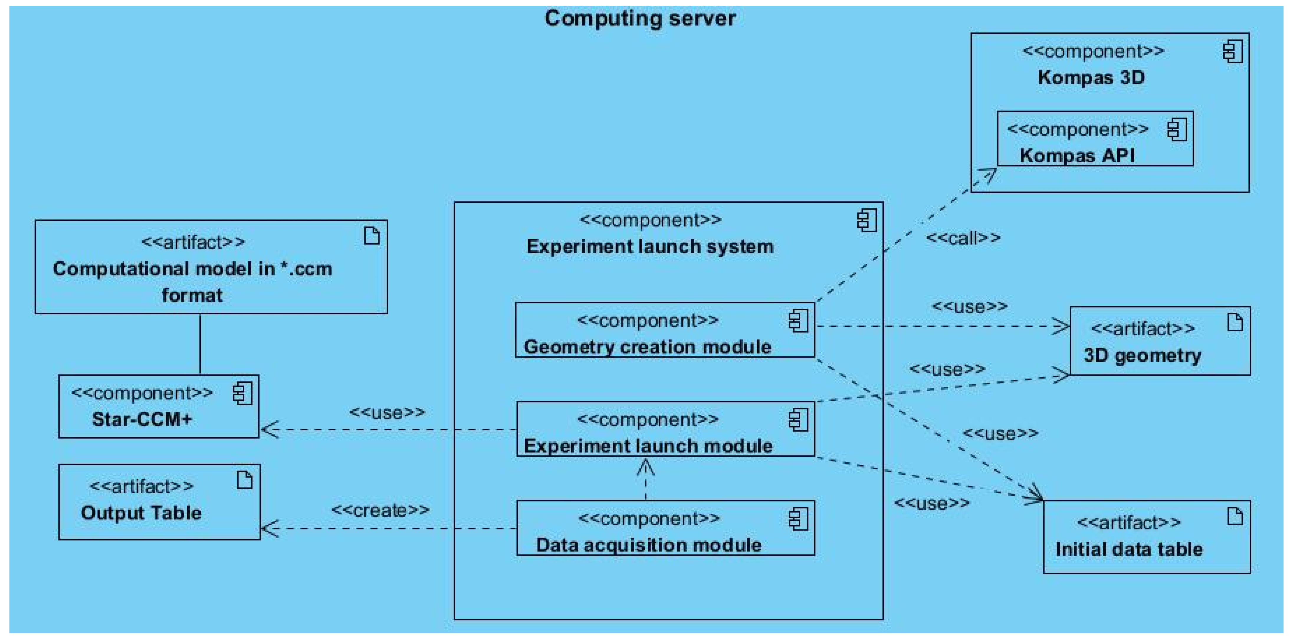
2.2. Automation System for Numerical Simulation of the Burner Operation

Since the application of machine learning technologies and methods requires a large amount of data, a specialized software package (SP) was developed. This SP automates the process of conducting numerical experiments by using a digital model of the burner device in a CFD system. It is a set of modules that implements software interfaces for interaction with CAD and CFD systems, and also allows the user to use a convenient graphical interface to configure the calculation parameters. The SP structure is presented as a deployment diagram in Figure 3. The system was developed using a Python 3.10 programming language.

At the input, this system receives a table of initial data with geometric parameters of the burner and the parameters of the combustion process simulation in the CFD system. Using a specialized macro via the Kompas API [53], the geometry creation module adjusts and builds a new geometry in the Kompas 3D CAD system, based on a 3D burner model template. Subsequently, the experiment launch module imports the resulting geometry into the Star-CCM+ numerical modeling system, makes the necessary settings for the grid and boundary conditions, sets the composition of the fuel, oxidizer and steam (the composition of the data is presented in

Table 1. Input parameters affecting the results of the burner operation (input data).

Symbol	Name	Unit of Measure	Minimum	Maximum
X1	Number of blades in the middle contour	pieces	9	36
X2	Number of blades in the outer contour	pieces	12	48
X3	The length of the blades in the outer contour	mm	44	108
X4	The angle of inclination of the blades in the outer contour	degree	30	75
X5	Primary air flow rate	m3/h	60.63	89.89
X6	Secondary air flow rate	m3/h	23.8	35.29
X7	Gas flow rate	kg/s	0.556	0.848
X8	Temperature	K	471	493
X9	Mass fraction $O_2$ in air	–	0.191	0.233
X10	Mass fraction $N_2$ in air	–	0.745	0.767
X11	Mass fraction $C{O}_2$ in air	–	0	0.022
X12	Amount of injected steam	%	0	5

) and starts the calculation process.

Furthermore, the data acquisition module saves all necessary data in form of graphs, a visual display of the combustion process and tables of output parameters. Subsequently, a single table is formed that contains both the input and output parameters obtained in the course of computational experiments, which are used in machine learning algorithms.

3. Application of Machine Learning Methods

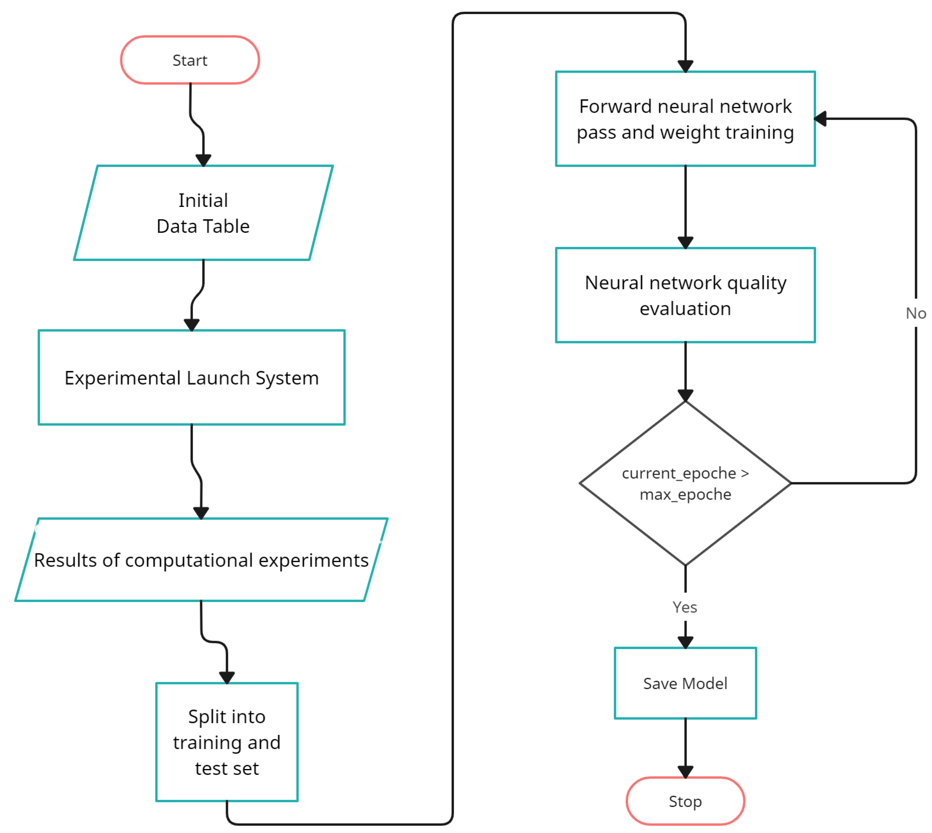
3.1. Deep Learning Problem Statement

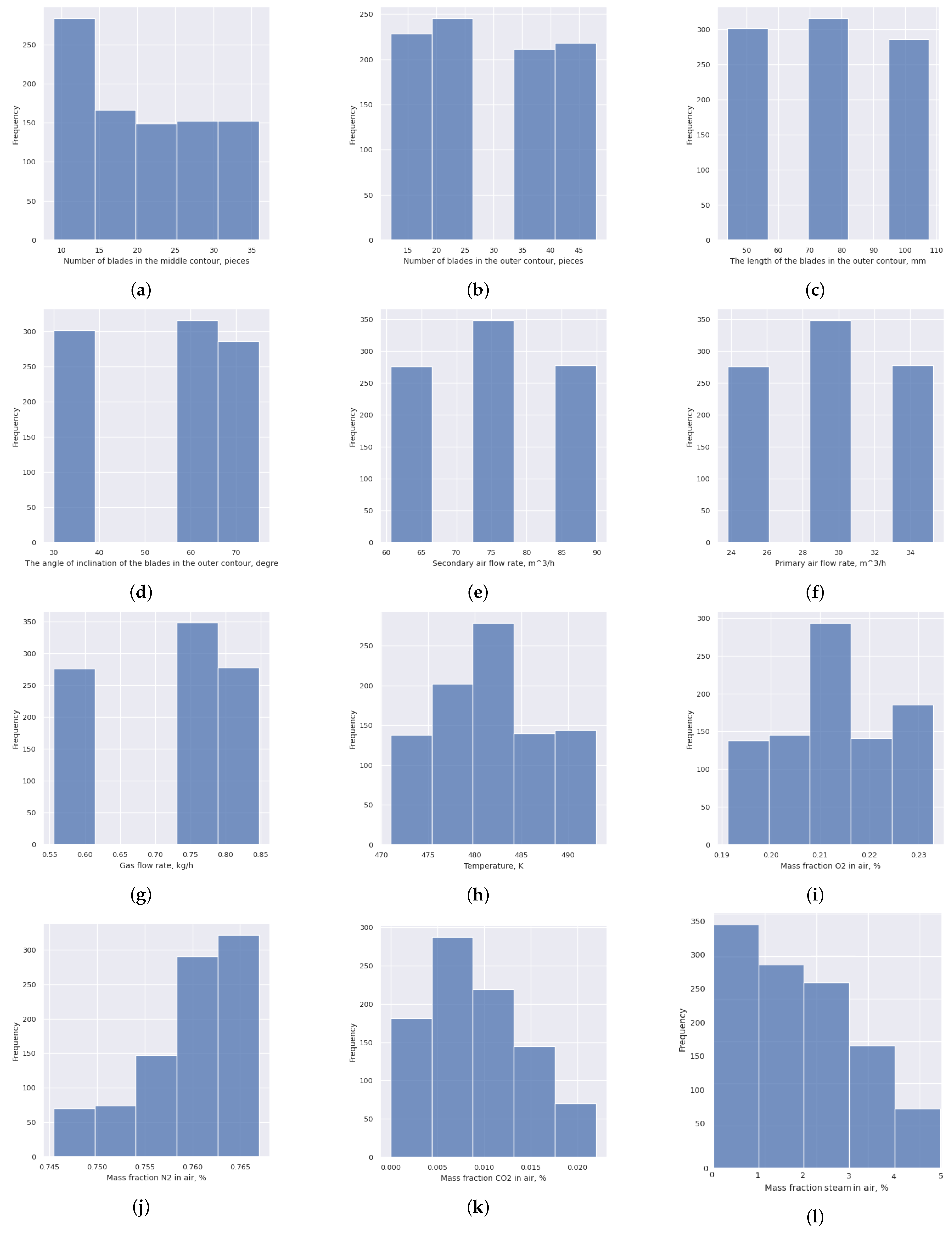
This paper discusses the use of deep learning methods in a burner device operation modeling based on data obtained during mathematical modeling of the combustion process. The operation of a burner device can be considered both from an environmental point of view, in the form of the amount of harmful substances emitted and from an economic point of view, in the form of efficiency, which is achieved at a given temperature.

To determine the relationship and optimal operation of the burner, a multiple regression model is used. For a given set of input parameters, a multiple regression model predicts a set of output parameters in the form of a non-linear dependence. A neural network is used as a tool to approximate the complex non-linear functions.

The use of neural networks instead of other machine learning methods is due to the ability to automatically extract features from input data. Unlike boosting, in which features are usually defined explicitly, neural networks can identify hidden dependencies and use them to build a model. In the context of multiple regression, boosting or other algorithms based on decision trees, forms multiple trees, each of which is created independently for each output parameter, thereby limiting the ability to account for their relationships.

3.2. Dataset

To eliminate scatter in the output data, these results were removed from the source data table. Therefore, the total amount of data for training and evaluating the ANN model were data from 1160 experiments. The description of the initial data is given in Table 1 and Figure 4.

The structure of the data obtained as a result of numerical experiments, taking into account the preliminary purification stage, is presented in

Table 2. Indicators obtained as a result of modeling (output data).

Symbol	Name	Unit of Measure	Minimum	Maximum
Y1	The position of the maximum temperature along the length of the combustion chamber	m	1.2	4.118
Y2	The maximum temperature of the combustion chamber	K	1901.728	2250.652
Y3	Distribution along the length of the combustion chamber of the maximum $N{O}_X$	m	1.271	4.617
Y4	Maximum mass fraction of $N{O}_X$ in the combustion chamber	%	0.000004	0.000383
Y5	Distribution along the length of the combustion chamber of the maximum $CO$	m	0.061	1.912
Y6	Maximum mass fraction of $CO$ in the combustion chamber	%	0.107	0.160
Y7	Distribution along the length of the combustion chamber of the maximum $C{O}_2$	m	1.414	4.332
Y8	Maximum mass fraction of $C{O}_2$ in the combustion chamber	%	0.108	0.125

.

The distributions of input and output data after excluding outliers are presented in the distribution diagrams (Figure 5 and Figure 6).

3.3. Data Pre-Processing

The neural network training process is an iterative process in which computations are performed forward and backward through each layer of the network until the loss function is minimized [54]. Before the training process, the data undergo a scaling procedure, which is an important step in the training process. This step is necessary to organize the data in such a way that they can be interpreted using mathematical models. This allows one to speed up training and improve the quality of the model. This study used the StandardScaler engine provided by the open source library scikit-learn. This mechanism transforms the data to center them by removing the mean of each feature and then scales them by dividing the non-constant features by their standard deviation. The standard score shows how many standard deviations of a given value are above or below the population or sample mean. The sample standard score (z) is calculated as follows [55]:

$$z={\displaystyle \frac{x-u}{s}}$$

where u—the mean of the training samples, or zero, s—standard deviation of the training samples or unit. Centering and scaling are performed independently for each function by identifying the relevant statistics for the indicators presented in the original data table. The mean and standard deviation are then stored for data scaling.

The use of the mathematical models and system to automate the numerical simulation of the burner operation is presented in Section 2, in which the geometric parameters of the burner and the parameters of the fuel composition were used as input parameters. During the study of the obtained data, outliers were found. This could worsen the quality indicators of the trained model. The example of an outlier is shown in Figure 7, where it can be seen that one experiment has a much bigger deviation from the average than all others. By pre-processing the entire set of presented data, such anomalous outliers were excluded with the help of specified filters when studying the output parameters presented in Table 2. After these manipulations, 1160 experimental data values were retained.

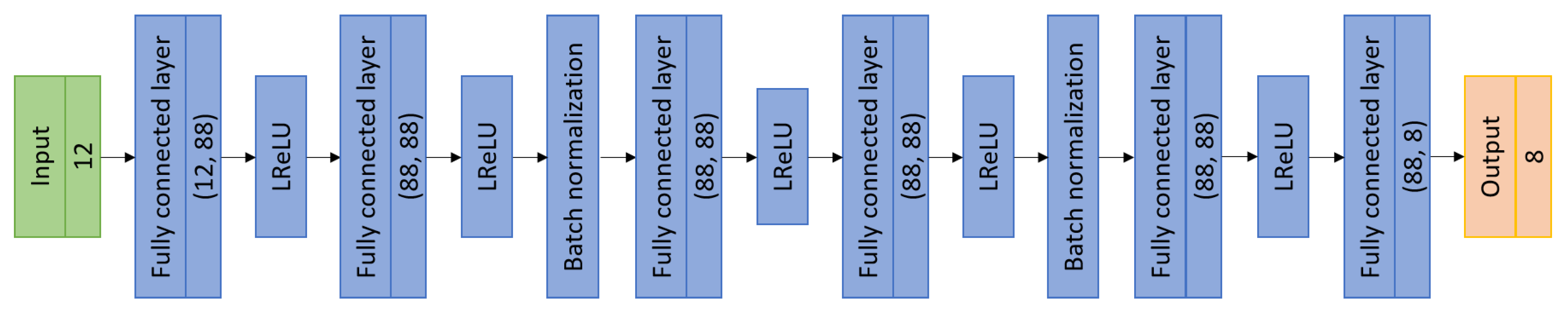
3.4. Artificial Neural Networks

Deep learning is currently one oaaf the most popular and promising areas in the field of machine learning. This approach is used for several tasks in the field of energy, such as determining combustion modes based on the analysis of images from the combustion chamber with the use of ultra-precise neural networks [56,57], detecting malfunctions in equipment with the use of recurrent neural networks [58,59,60,61] and energy generation forecasts [62]. For multiple regression, a deep feed-forward neural network is used, which is called a multilayer perceptron (MLP). An MLP is a set of connected layers consisting of many artificial neurons. An MLP consists of an input layer, several hidden layers and an output layer. Mathematically, the hidden layer can be represented as follows:

$$y=W^T\times x+b,$$

where $W^T$—a weight matrix, which is a set of training parameters, and encodes information about the relationships between data in the subject area, x—a set of input parameters coming from the previous layer, in the case of the first hidden layer, the input parameters are the original data, and b—a bias. Values obtained from one hidden layer are normalized using an activation function before being passed to the next. All weights and biases are solved using the back-propagation method [63]. This is necessary in order to enable the ANN to build non-linear dependencies.

The activation function can be represented as follows:

Rectified linear unit (ReLU):

$$ReLU\left(y\right)=\left\{\begin{array}{c}0, y<0\hfill \\ y, y\ge 0\hfill \end{array}\right.$$

Leaky rectified linear unit (LReLU):

$$LReLU\left(y\right)=\left\{\begin{array}{c}0.01\times y, y<0\hfill \\ y, y\ge 0\hfill \end{array}\right.$$

Tangent hyperbolic (Tanh):

$$Tanh\left(y\right)={\displaystyle \frac{e^y-e^{-y}}{e^y+e^{-y}}}$$

Sigmoid:

$$\sigma \left(y\right)={\displaystyle \frac{1}{1+e^{-y}}}$$

Network training occurs by minimizing the loss function, which is calculated after each pass of the network and shows its quality in a given training step, and comparing real data with predicted ones. After that, the weights are updated, aimed at reducing the value of the loss function. As a rule, gradient descent methods [64] are used for this.

The complete scheme to model the burner operation parameters with subsequent training of the neural network model is shown in Figure 8.

This approach made it possible to reduce the time for conducting experiments and also, with the help of a trained neural network model, to speed up the process of selecting the burner parameters to determine its optimal operation.

Since the problem of multiple regression is being solved within the framework of this work, the multi-layer perceptron (MLP) will be used as a neural network model, to predict the operating modes of the burner device based on the specified parameters. The architecture of the developed ANN is shown in Figure 9. In this case, we had 12 input parameters that were passed from the input layer to the first hidden layer. For the best quality ANN model, we empirically selected 88 artificial neurons on each hidden layer. Eight output parameters were determined based on the efficiency of the burner device. These options were presented above. The open source Pylibrary [65] in Python was used to implement the ANN.

It is also worth noting that a normalization layer was used to prevent ANN retraining [66]:

$$y={\displaystyle \frac{x-E\left[x\right]}{\sqrt{Var\left[x\right]+ϵ}}}\times \gamma +\beta$$

where x—input values of the layer, $E\left[x\right]$—mean value, $Var\left[x\right]$—variance, $ϵ$—a random variable, excluding division by 0, in the case of $Var\left[x\right]$ = 0, and usually takes quite low values, $\gamma$ and $\beta$ are learning parameters that are used to scale and shift the normalized values.

This layer allowed us to increase the quality of the model being trained with a large number of hidden layers.

3.5. Model Comparison

The learning rate, a hyperparameter that is used to train neural networks, is mostly in the range from 0.0 to 1.0. The learning rate shows how fast the model adapts to the problem presented. Lower learning rates require more training epochs, given the smaller changes made to the weights with each update, while higher learning rates result in faster changes and require fewer training epochs [67]. The following values were set as hyperparameters:

• Training set: 928 samples (80% data);
• Test set: 232 samples (20% data);
• Optimizer: Pytorch Adam;
• Loss function: Pytorch MSE;
• Learning rate: 0.01;
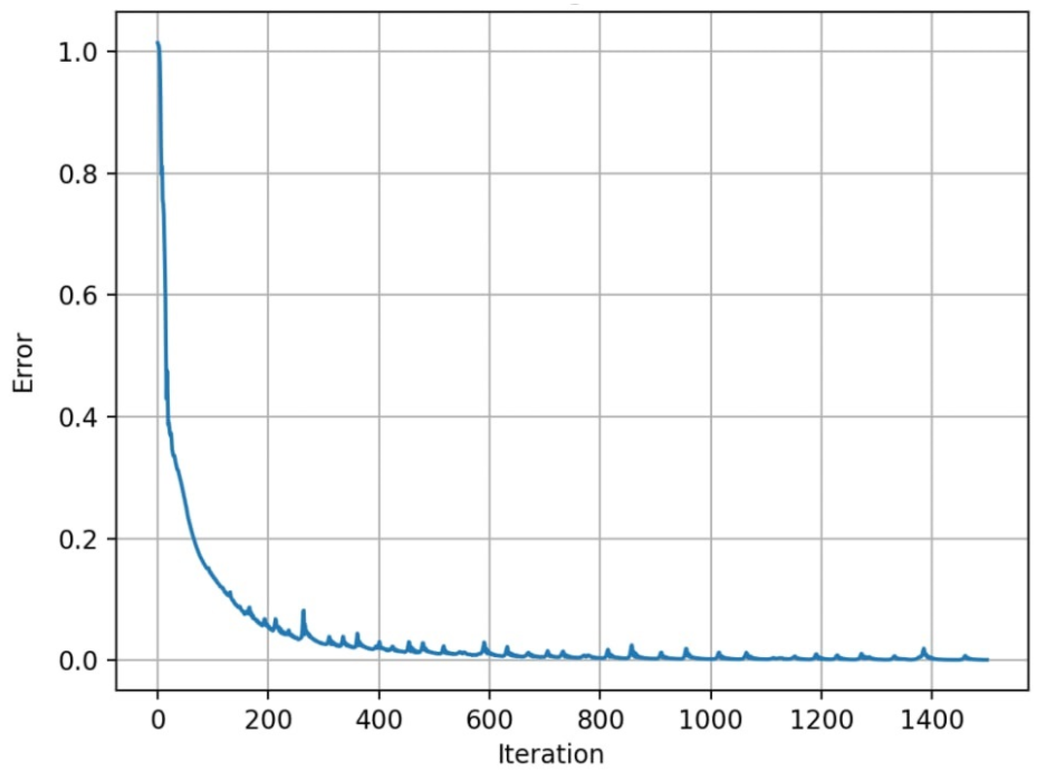
• Epochs: 1500.

These hyperparameters and architecture were chosen empirically, for minimizing the loss function in the learning process. The use of an 80/20 data split proportion without creating a separate validation set is due to the limited amount of available data, which made it possible to reduce the overall error in the training process and obtain an appropriate result in the test dataset. This can be explained by the fact that, during the training process, the neural network received more examples. As a result, it was able to better approximate the non-linear relationship between the data.

To assess the quality of deep learning models in multiple regression problems, the following indicators are used: MAE, mean absolute error; MSE, mean square error; and RMSE, root mean square error. The definitions of these equations are given in the following expressions:

$$MAE={\displaystyle \frac{1}{n}}\sum _{i=1}^n|\widehat{Y_i}-Y_i|$$

$$MSE={\displaystyle \frac{1}{n}}\sum _{i=1}^n{(\widehat{Y_i}-Y_i)}^2$$

$$RMSE=\sqrt{{\displaystyle \frac{1}{n}}\sum _{i=1}^n{(\widehat{Y_i}-Y_i)}^2}$$

where n—the number of data samples, $\widehat{Y_i}$—values predicted by neural network, $Y_i$—actual value.

The MSE function is also used in the ANN learning process as a loss function.

The learning process, a decrease in the error in terms of MSE at each training epoch, is shown in Figure 10. When training a neural network, the error decreases at each iteration. The number of iterations was chosen empirically when the required degree of learning was achieved.

The results of accuracy check of the developed neural network model on test data are presented in

Table 3. Results of checking the ANN model on the test set.

Parameter	MAE	MSE	RMSE
Flame core position	0.155	0.049	0.220
Flame core temperature	14.931	472.134	21.729
Maximum $N{O}_X$ distribution function	0.214	0.094	0.306
Maximum mass fraction of $N{O}_X$	$9.457\times {10}^{-6}$	$3.036\times {10}^{-10}$	$1.742\times {10}^{-5}$
Maximum $CO$ distribution function	0.207	0.079	0.281
Maximum mass fraction of $CO$	0.005	$4.990\times {10}^{-5}$	0.007
Maximum $C{O}_2$ distribution function	0.179	0.054	0.233
Maximum mass fraction of $C{O}_2$	0.002	$6.502\times {10}^{-6}$	0.003

.

Also, an example of the predicted indicators in the test sample for the maximum mass fraction of $N{O}_X$ and the temperature of the flame core are shown in Figure 11—comparison of $N{O}_X$ distribution as a function of flame core temperature. It is known that thermal $N{O}_X$ is formed as a result of high temperatures in the flame core; thus, the figure shows an adequate prediction of $N{O}_X$ formation.

As shown, the results obtained have relatively small deviations, which indicates that the ANN can be used as a model that describes the relationship between the burner device parameters and its operating modes.

To check the model correctness, the quality of its work was compared with other common methods used in regression problems, such as boosting and SVR [54]. Boosting is a method used in machine learning to reduce errors in predictive data analysis. The SVR method allows you to define a function that approximates the relationship between input variables and a continuous target variable, while minimizing the prediction error. To implement boosting, the CatBoost library was used [68], and to implement SVR—the scikit-learn library [55]. To implement multiple regression using these methods, parallel construction of the models was implemented using the following parameters:

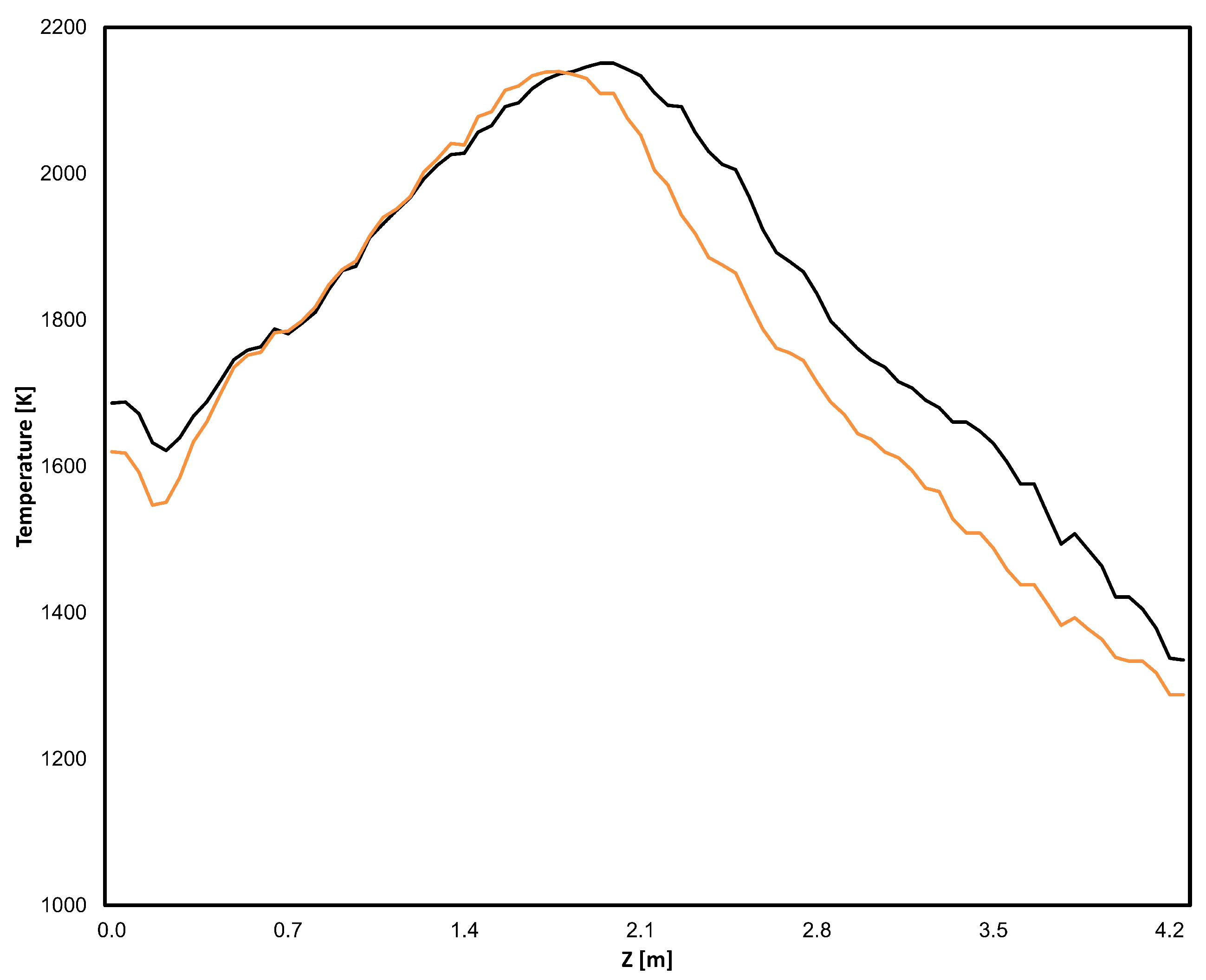
• Flame core position;
• Flame core temperature;
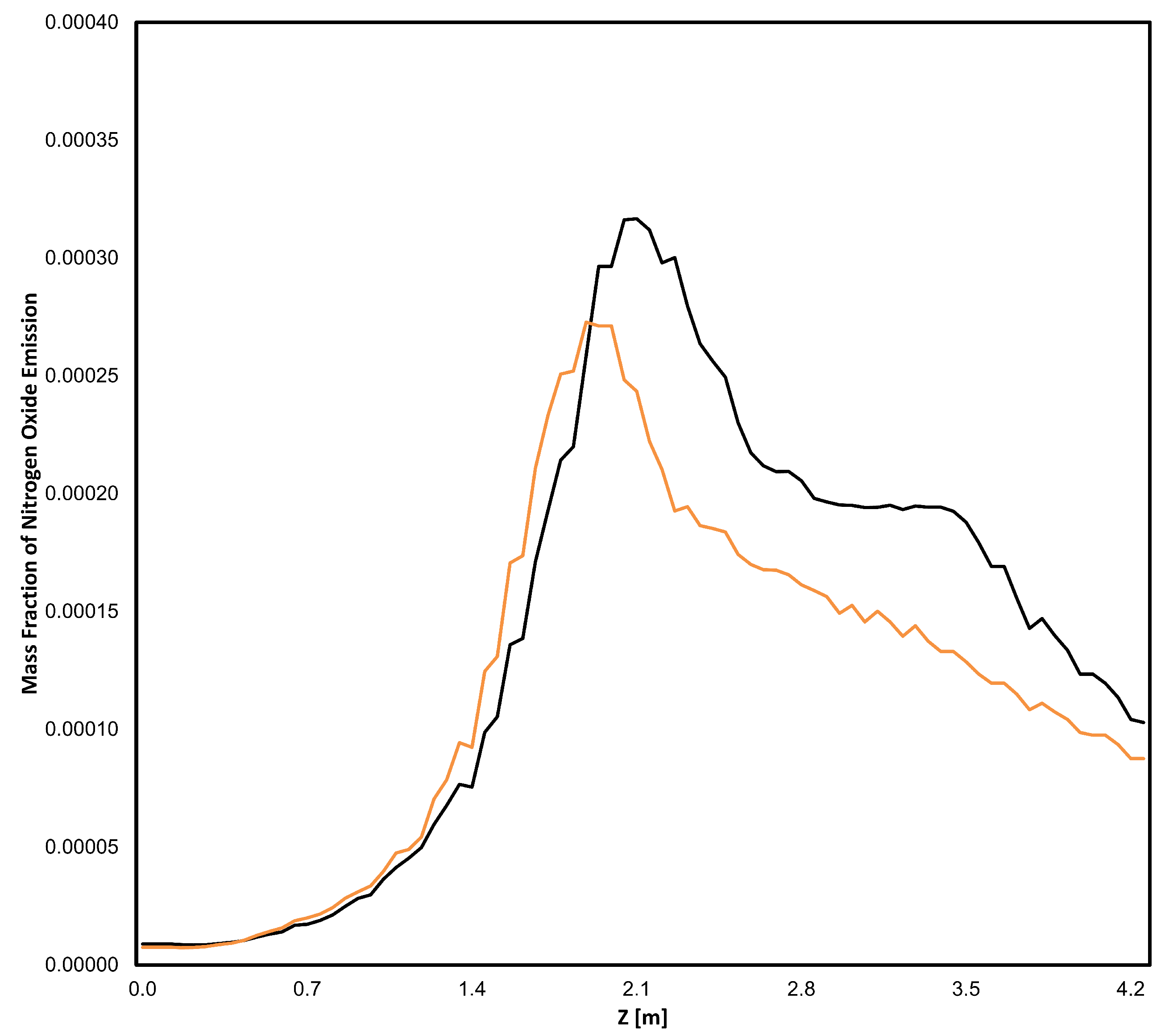
• Maximum $N{O}_X$ distribution function;
• Maximum mass fraction of $N{O}_X$.

The results of the model quality comparison are presented in

Table 4. Results of the quality comparison of the models on the test set.

Parameter	ANN			CatBoost			SVR
	MAE	MSE	RMSE	MAE	MSE	RMSE	MAE	MSE	RMSE
Flame core position	0.155	0.049	0.220	0.161	0.056	0.237	0.167	0.061	0.247
Flame core temperature	14.931	472.134	21.729	14.631	470.871	21.7	16.129	474.237	21.78
Maximum $N{O}_X$ distribution function	0.214	0.094	0.306	0.221	0.099	0.315	0.224	0.103	0.321
Maximum mass fraction of $N{O}_X$	$\mathbf{9}.\mathbf{457}\times {\mathbf{10}}^{-\mathbf{6}}$	$\mathbf{3}.\mathbf{036}\times {\mathbf{10}}^{-\mathbf{10}}$	$\mathbf{1}.\mathbf{742}\times {\mathbf{10}}^{-\mathbf{5}}$	$9.465\times {10}^{-6}$	$3.043\times {10}^{-10}$	$1.744\times {10}^{-5}$	$9.472\times {10}^{-6}$	$3.049\times {10}^{-10}$	$1.746\times {10}^{-5}$

.

As can be seen from Table 4, the best results were obtained by the ANN. This result shows the distinctive feature of an artificial neural network that is capable of predicting multiple output values based on all input values, while Boosting and SVR can only predict one output value, which leads to a loss of connection between the input and output values and a decrease in the accuracy of the results obtained.

4. Results and Discussion of Parameter Optimization Using a Trained ANN

For functions consisting of many parameters that need to be optimized, methods such as gradient descent, particle swarming or genetic algorithm are currently used [64]. The gas burner must primarily ensure a decrease in temperature and reliable mixing of air with fuel to prevent incomplete chemical combustion of the fuel and flame detachment. During the reconstruction of burner devices for operating steam boilers of thermal power plants during technical re-equipment and reconstruction, it is possible not only to improve the technical and economic indicators of the legal boiler and to increase the safety of its operation, but also to simultaneously achieve a decrease in $N{O}_X$ emissions. Often, during the technical re-equipment of operating burner devices of steam boilers in thermal power plants, the transition to a low-emission device is carried out together with other methods. A study on reducing in $N{O}_X$ emissions with exhaust gases from steam boilers of thermal power plants is relevant because it aims at solving the fundamental scientific problem of understanding the patterns of heat and mass transfer and fluid dynamics processes. It provides the possibility for identifying patterns of efficiency and environmentally friendly combustion of organic fuel in steam boilers of thermal power plants and boiler houses, and allows for the development of environmentally friendly solutions and modern technologies in the energy sector. In this study, gradient descent was used to optimize the burner parameters. The essence of this approach is to find the local minimum of the function in the direction of the steepest descent and to output the parameters that led to the minimum value. The trained ANN considered in the previous sections acted as a function of the set of input parameters. The gradient was calculated using the following equation:

$${\Theta }_t={\Theta }_{t-1}-a\times g_t$$

where: ${\Theta }_t$—model parameters per iteration t, t—descent iteration number, a—learning rate, $g_t$—gradient offset value per iteration t.

This method is the simplest to implement local optimization and allows you to determine the optimal burner input parameters using ANNs in order to minimize output values (such as the mass fraction of $N{O}_X$), while considering the behavior of other output parameters that correspond to this mode of operation.

In order to optimize $N{O}_X$ emissions, the parameters that could influence the burner operation and those related to the design characteristics were investigated. Optimization was carried out using the basic values corresponding to the accepted mode of operation and the current design of the burner:

• Primary air quantity—60.63 m/s;
• Mass flow rate of fuel (methane)—0.556 kg/s;
• Number of blades in the middle contour—18;
• Number of blades in the outer contour—24;
• The length of the blades in the outer contour—70 mm;
• The angle of inclination of the blades in the outer contour—60 degrees.

For each parameter, search ranges for the best options were set. For the amount of primary air and the mass flow rate of the fuel, the search boundary conditions were set in the range of ±10% of the base values. The search range of the geometric parameters was set as follows:

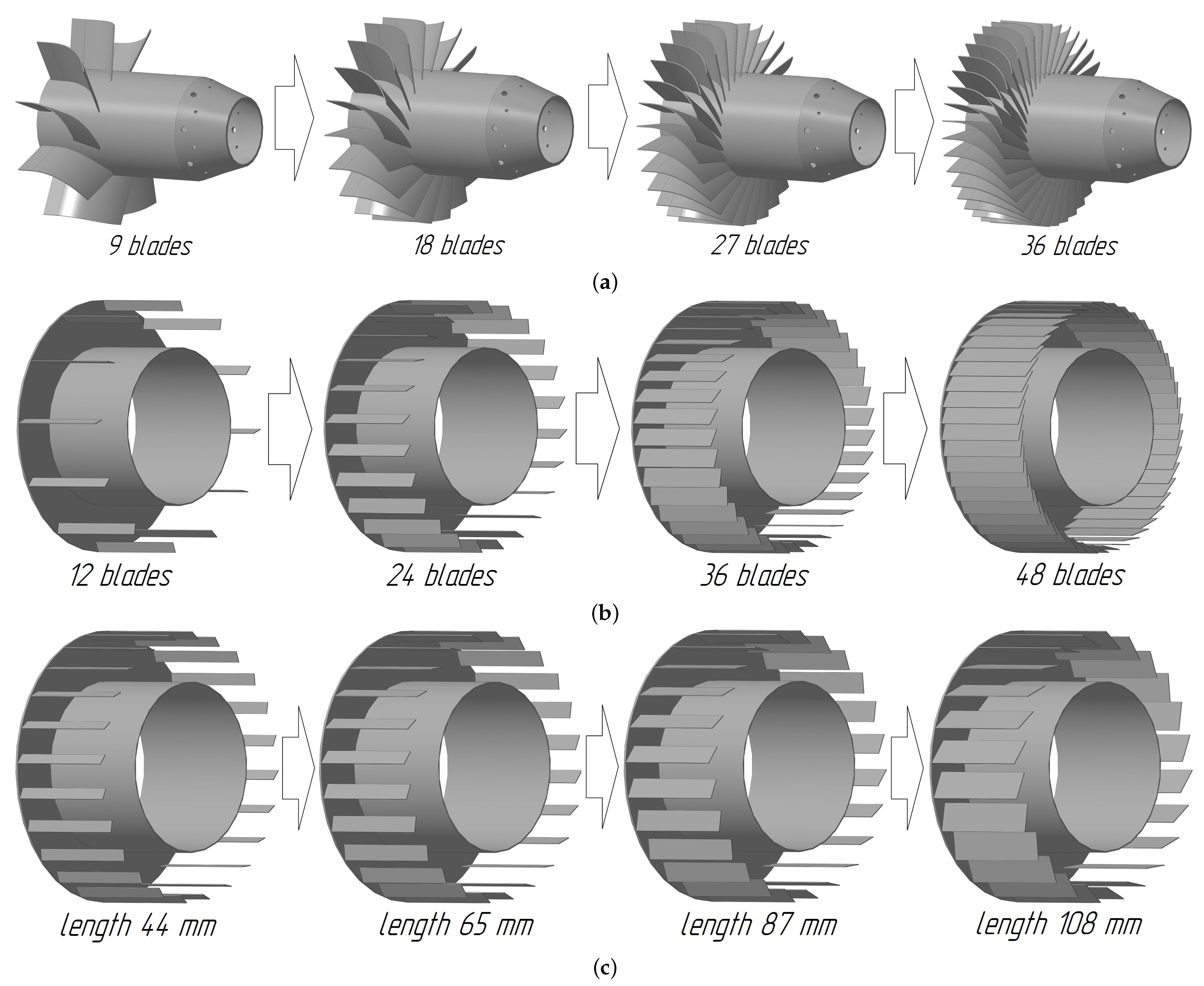
• Number of blades in the middle contour: from 9 to 36;
• Number of blades in the outer contour: from 12 to 48;
• The length of the blades in the outer contour: from 44 to 108 mm;
• The angle of inclination of the blades in the outer contour: from 30 to 75 degrees.

In the course of applying this approach, the following results were obtained, presented in

Table 5. Results of checking the ANN model on the test set.

Primary Air Flow Rate	Gas Flow Rate	Number of Blades in the Middle Contour	Number of Blades in the Outer Contour	The Length of the Blades in the Outer Contour	The Angle of Inclination of the Blades in the Outer Contour	Steam Content in the Air
65.73	0.584	16	28	44	63	5

.

The obtained data were tested in the Star-CCM+ environment, where, as a result of a numerical experiment, profiles of the distribution of values along the combustion chamber were obtained, which are presented in Figure 12, Figure 13, Figure 14 and Figure 15. The initial data for the figures were the values taken along the central axis of the burner device along the entire length of the combustion chamber. For comparison, the principle of uniformity of measurements was observed by bringing the measured values to standard conditions with a conditional excess air ratio of $1.4$ (which corresponds to an oxygen concentration in the flue gases of 6%).

For comparison, the principle of measurement uniformity was maintained by adjusting the measured values to standard conditions with a nominal excess air ratio of 1.4 (equivalent to an oxygen concentration of 6% in the flue gases). As shown in Figure 12, changes in the mass flow rates of primary air, steam and fuel, as well as geometric parameters, affect the temperature of the flame core and shift it along the flow direction. This is due to the fact, owing to changes in parameters, the resistance in the air path decreases, the flame stretches and combustion occurs in a larger volume. An increase in the angle of the blades led to an increase in the swirl of the flame. At the same time, as can be seen in Figure 13, an increase in the mass flow rate of the fuel and primary air when changing the geometric parameters can lead to a decrease in the maximum concentration of $N{O}_X$ with a slight decrease in temperature, which makes it possible to achieve higher environmental performance while maintaining energy efficiency. In addition, fuel composition and geometry control can reduce $CO$ levels and influence the amount and location of $C{O}_2$ concentration, as shown in Figure 14 and Figure 15.

If we compare the maximum values of $N{O}_X$ concentration along the combustion chamber, which were $3.167\times {10}^{-4}$ in the basic calculation and $2.727\times {10}^{-4}$ in the calculation with the optimized values, we can conclude that changing the fuel composition with a change in the burner design allows us to achieve a reduction in $N{O}_X$ level of approximately 15%.

It should be noted that the results of numerical simulation revealed a rather non-linear relationship between input values and output values. This is largely owing to the complex processes occurring in the swirling flow in the burner device.

The artificial neural network provided accurate results, indicating the potential for its reliable application in assessing the efficiency of the fuel combustion process in burner devices. The results of our study can also be used to modify and develop low-emission burner devices. Most importantly, the results of our study can provide guidance for future joint applications of CFD and machine learning models in various energy facilities to evaluate combustion efficiency. It should also be noted that prediction beyond the range of the training data is a common limitation for all machine learning models.

5. Conclusions

This study addressed mathematical modeling and a numerical study of turbulent gas flow in the STAR-CCM+ multidisciplinary platform. Traditional methods, including CFD, are often resource-intensive and time-consuming. Numerical modeling allows for a detailed analysis of the processes under study, but simultaneously requires significant computing resources, especially when modeling complex three-dimensional flows and non-stationary processes. Unlike CFD, ANNs have the potential to learn from available data, quickly make predictions and adapt to changing conditions, which is confirmed by a significant amount of work devoted to the use of ANNs in the study of fluid dynamics. An automated system was also developed to conduct experiments using a numerical model of the burner. Based on the obtained results, a neural network model was trained, and for this purpose the architecture and hyperparameters were selected experimentally. Using such a model, a number of experiments were carried out to find suitable parameters for a heating device to optimize the combustion temperature while minimizing harmful emissions. The combination of operating and design characteristics turned out to be the most optimal, which, while maintaining a high temperature, made it possible to reduce the amount of $N{O}_X$ emissions. Thus, the use of the neural network approach made it possible to develop recommendations and proposals for the modernization and adjustment of burners to reduce the harmful emissions. This study examines the possibility of using trainable artificial neural networks to simulate and optimize a burner device used in one of the most common steam boilers in the Russian energy sector, which provides a wide opportunity to scale the obtained results and achieve significant technical and socially oriented results, including paying attention to reducing $N{O}_X$ emissions.

The results of processing showed the most significant effect on the $N{O}_X$ content, which is exerted by a change in the mass flow rate of primary air and fuel with a change in geometric parameters. The decrease in $N{O}_X$ concentration compared with the calculation results with basic values was approximately 15%. This is achieved by decreasing the temperature in the core of the flame and improving the mixing of the fuel–air mixture as a result of changing the geometric characteristics. The results obtained form the basis for decision-making when modeling the combustion process using machine learning in boilers with various designs and performances.

References

1. Senyuk, M.D.; Dmitrieva, A.A. Development of the method for dynamic stability assessment of power systems based on the application of the artificial intelligence theory taking into account the topological connectivity of the network. Electrotech. Syst. Complexes 2022, 4, 12–19. [Google Scholar] [CrossRef]
2. Sartor, K.; Sylvain, Q.; Pierre, D. Simulation and optimization of a CHP biomass plant and district heating network. Appl. Energy 2014, 130, 474–483. [Google Scholar] [CrossRef]
3. Xu, B.; Wang, J.; Wang, X.; Liang, Z.; Cui, L.; Liu, X.; Ku, A.Y. A case study of digital-twin-modelling analysis on power-plant-performance optimizations. Clean Energy 2019, 3.3, 227–234. [Google Scholar] [CrossRef]
4. Baukal, C.E., Jr. Oxygen-Enhanced Combustion; CRC Press: Boca Raton, FL, USA, 2010. [Google Scholar]
5. Shaw, S.; Van Heyst, B. An Evaluation of Risk Ratios on Physical and Mental Health Correlations due to Increases in Ambient Nitrogen Oxide (NOX) Concentrations. Atmosphere 2022, 13, 967. [Google Scholar] [CrossRef]
6. Varaksin, A.Y.; Ryzhkov, S.V. Particle-laden and droplet-laden two-phase flows past bodies (a review). Symmetry 2023, 15, 388. [Google Scholar] [CrossRef]
7. Pakhomov, M.A.; Terekhov, V.I. Effect of the Shape of Pulses on Heat Transfer at the Stagnation Point of a Nonstationary Axisymmetric Impact Gas–Droplet Jet. J. Eng. Phys. Thermophys. 2022, 95, 985–990. [Google Scholar] [CrossRef]
8. Hibiki, T.; Tsukamoto, N. Drift-flux model for upward dispersed two-phase flows in vertical medium-to-large round tubes. Prog. Nucl. Energy 2023, 158, 104611. [Google Scholar] [CrossRef]
9. Guo, Q.; Liu, H.L.; Xie, G.; Guo, C.; Xu, Z.; Shao, X.D. Investigation on the two-phase flow and heat transfer behaviors in a new central uniform dispersion-type heat exchanger. Int. Commun. Heat Mass Transf. 2022, 137, 106283. [Google Scholar] [CrossRef]
10. Bamidele, O.E.; Ahmed, W.H.; Hassan, M. Characterizing two-phase flow-induced vibration in piping structures with U-bends. Int. J. Multiph. Flow 2022, 151, 104042. [Google Scholar] [CrossRef]
11. Hundshagen, M.; Rave, K.; Nguyen, B.D.; Popp, S.; Hasse, C.; Mansour, M.; Thévenin, D.; Skoda, R. Two-phase flow simulations of liquid/gas transport in radial centrifugal pumps with special emphasis on the transition from bubbles to adherent gas accumulations. J. Fluids Eng. 2022, 144, 101202. [Google Scholar] [CrossRef]
12. Zhang, J.; Lou, W.; Shao, P.; Zhu, M. Mathematical simulation of impact cavity and gas–liquid two-phase flow in top–bottom blown converter with Eulerian-multifluid VOF model. Metall. Mater. Trans. B 2022, 53, 3585–3601. [Google Scholar] [CrossRef]
13. Tas, S. A comprehensive review of numerical and experimental research on the thermal-hydraulics of two-phase flows in vertical rod bundles. Int. J. Heat Mass Transf. 2024, 221, 125053. [Google Scholar] [CrossRef]
14. Yao, Y.; Hrnjak, P. Developing adiabatic two-phase flow after an expansion valve: Flow development in an 8 mm tube. Int. J. Refrig. 2023, 149, 83–93. [Google Scholar] [CrossRef]
15. Kocar, C.; Sokmen, C.N. A CFD model of two-phase flow in BWRs with results of sensitivity and uncertainty analysis. Nucl. Eng. Des. 2009, 239, 1839–1846. [Google Scholar] [CrossRef]
16. Askarova, A.S.; Bolegenova, S.A.; Maximov, V. 3D visualization of the results of using modern OFA technology on the example of real boiler. WSEAS Trans. Fluid Mech. 2021, 16, 232–238. [Google Scholar] [CrossRef]
17. Aversano, G.; Marco, F.; Parente, A. Digital twin of a combustion furnace operating in flameless conditions: Reduced-order model development from CFD simulations. Proc. Combust. Inst. 2021, 38, 5373–5381. [Google Scholar] [CrossRef]
18. Chernov, A.A.; Maryandyshev, P.A.; Pankratov, E.V.; Lubov, V.K. CFD simulation of the combustion process of the low-emission vortex boiler. J. Phys. Conf. Ser. 2017, 891, 012216. [Google Scholar] [CrossRef]
19. Karim, M.; Arafat, A.; Naser, J. CFD simulation of biomass thermal conversion under air/oxy-fuel conditions in a reciprocating grate boiler. Renew. Energy 2020, 146, 1416–1428. [Google Scholar] [CrossRef]
20. Slotnick, J.P.; Khodadoust, A.; Alonso, J.; Darmofal, D.; Gropp, W.; Lurie, E.; Mavriplis, D.J. CFD Vision 2030 Study: A Path to Revolutionary Computational Aerosciences. 2014. No. NF1676L-18332. Available online: https://ntrs.nasa.gov/citations/20140003093 (accessed on 26 January 2025).
21. Chen, S.; Xing, Y.; Li, A. CFD investigation on Low-NOX strategy of folded flame pattern based on fuel-staging natural gas burner. Appl. Therm. Eng. 2017, 112, 1487–1496. [Google Scholar] [CrossRef]
22. Rossiello, G.; Uzair, M.A.; Ahmadpanah, S.B.; Morandi, L.; Ferrara, M.; Rago, G.D.; Torresi, M. Design and testing of a Multi-Fuel industrial burner suitable for syn-gases, flare gas and pure hydrogen. Therm. Sci. Eng. Prog. 2023, 42, 101845. [Google Scholar] [CrossRef]
23. Chapela, S.; Porteiro, J.; Gómez, M.A.; Patiño, D.; Míguez, J.L. Comprehensive CFD modeling of the ash deposition in a biomass packed bed burner. Fuel 2018, 234, 1099–1122. [Google Scholar] [CrossRef]
24. Garcia, A.M.; Rendon, M.A.; Amell, A.A. Combustion model evaluation in a CFD simulation of a radiant-tube burner. Fuel 2020, 276, 118013. [Google Scholar] [CrossRef]
25. Wang, Y.; Xu, W. A novel decision optimization for thermal power unit based on condition-based predictive maintenance and equilibrium optimizer. Phys. Commun. 2024, 65, 102372. [Google Scholar] [CrossRef]
26. Wang, Z.; Liu, M.; Yan, H.; Zhao, Y.; Yan, J. Improving flexibility of thermal power plant through control strategy optimization based on orderly utilization of energy storage. Appl. Therm. Eng. 2024, 240, 122231. [Google Scholar] [CrossRef]
27. Kůdela, J.; Suja, J.; Šomplák, R.; Pluskal, J.; Hrabec, D. Optimal control of combined heat and power station operation. Optim. Eng. 2024, 25, 121–145. [Google Scholar] [CrossRef]
28. Wang, Q.; Leng, Z.; Tan, H.; Mohamed, M.A.; Jin, T. Optimal scheduling of virtual power plants with reversible solid oxide cells in the electricity market. Renew. Energy 2024, 237, 121759. [Google Scholar] [CrossRef]
29. Wu, S.; Wang, Y.; Liu, L.; Yang, Z.; Cao, Q.; He, H.; Cao, Y. Two-stage distributionally robust optimal operation of rural virtual power plants considering multi correlated uncertainties. Int. J. Electr. Power Energy Syst. 2024, 161, 110173. [Google Scholar] [CrossRef]
30. Deon, B.; Cotta, K.P.; Silva, R.F.V.; Batista, C.B.; Justino, G.T.; Freitas, G.C.; Padoin, N. Digital twin and machine learning for decision support in thermal power plant with combustion engines. Knowl.-Based Syst. 2022, 253, 109578. [Google Scholar] [CrossRef]
31. Ahmed, I.; Rehan, M.; Basit, A.; Hong, K.S. Greenhouse gases emission reduction for electric power generation sector by efficient dispatching of thermal plants integrated with renewable systems. Sci. Rep. 2022, 12, 12380. [Google Scholar] [CrossRef]
32. Mahdavipour, P.; Wiel, C.; Spliethoff, H. Optimal control of combined-cycle power plants: A data-enabled predictive control perspective. IFAC-PapersOnLine 2022, 55, 91–96. [Google Scholar] [CrossRef]
33. Brunton, S.L.; Noack, B.R.; Koumoutsakos, P. Machine learning for fluid mechanics. Annu. Rev. Fluid Mech. 2020, 52, 477–508. [Google Scholar] [CrossRef]
34. Klyachkin, V.N.; Kuvayskova, J.E.; Zhukov, D.A. Aggregated classifiers for state diagnostics of the technical object. In Proceedings of the International Multi-Conference on Industrial Engineering and Modern Technologies (FarEastCon), Vladivostok, Russia, 1–4 October 2019. [Google Scholar]
35. Breiman, L. Classification and Regression Trees, 1st ed.; Routledge: London, UK, 2017. [Google Scholar]
36. Chen, T.; Guestrin, C. XGBoost: A Scalable Tree Boosting System. In Proceedings of the 22nd ACM SIGKDD International Conference on Knowledge Discovery and Data Mining (KDD ’16). Association for Computing Machinery, New York, NY, USA, 13–17 August 2016; pp. 785–794. [Google Scholar]
37. Alshboul, O.; Shehadeh, A.; Mamlook, R.E.A.; Almasabha, G.; Almuflih, A.S.; Alghamdi, S.Y. Prediction Liquidated Damages via Ensemble Machine Learning Model: Towards Sustainable Highway Construction Projects. Sustainability 2021, 14, 9303. [Google Scholar] [CrossRef]
38. Shehadeh, A.; Alshboul, O.; Al Mamlook, R.E.; Hamedat, O. Machine learning models for predicting the residual value of heavy construction equipment: An evaluation of modified decision tree, LightGBM, and XGBoost regression. Autom. Constr. 2021, 129, 103827. [Google Scholar] [CrossRef]
39. Abdul Jameel, A.G.; Al-Muslem, A.; Ahmad, N.; Alquaity, A.B.S.; Zahid, U.; Ahmed, U. Predicting Enthalpy of Combustion Using Machine Learning. Processes 2022, 10, 2384. [Google Scholar] [CrossRef]
40. Krayden, A.; Schohet, M.; Shmueli, O.; Shlenkevitch, D.; Blank, T.; Stolyarova, S.; Nemirovsky, Y. CMOS-MEMS Gas Sensor Dubbed GMOS for SelectiveAnalysis of Gases with Tiny Edge Machine Learning. Eng. Proc. 2022, 27, 81. [Google Scholar] [CrossRef]
41. Brusa, A.; Giovannardi, E.; Barichello, M.; Cavina, N. Comparative Evaluation of Data-Driven Approaches to Develop an Engine Surrogate Model for NOX Engine-Out Emissions under Steady-State and Transient Conditions. Energies 2022, 15, 8088. [Google Scholar] [CrossRef]
42. Zhang, H.; Lu, H.; Xie, F.; Ma, T.; Qian, X. Combustion Regime Identification in Turbulent Non-Premixed Flames with Principal Component Analysis, Clustering and Back-Propagation Neural Network. Processes 2022, 10, 1653. [Google Scholar] [CrossRef]
43. Yang, R.; Xie, T.; Liu, Z. The Application of Machine Learning Methods to Predict the Power Output of Internal Combustion Engines. Energies 2022, 15, 3242. [Google Scholar] [CrossRef]
44. Yang, R.; Yan, Y.; Sun, X.; Wang, Q.; Zhang, Y.; Fu, J.; Liu, Z. An Artificial Neural Network Model to Predict Efficiency and Emissions of a Gasoline Engine. Processes 2022, 10, 204. [Google Scholar] [CrossRef]
45. Bai, M.; Liu, J.; Ma, Y.; Zhao, X.; Long, Z.; Yu, D. Long Short-Term Memory Network-Based Normal Pattern Group for Fault Detection of Three-Shaft Marine Gas Turbine. Energies 2021, 14, 13. [Google Scholar] [CrossRef]
46. Kuzhagaliyeva, N.; Horváth, S.; Williams, J.; Nicolle, A.; Sarathy, S.M. Artificial intelligence-driven design of fuel mixtures. Commun. Chem. 2022, 5, 111. [Google Scholar] [CrossRef] [PubMed]
47. Raissi, M.; Perdikaris, P.; Karniadakis, G.E. Physics informed deep learning (part i): Data-driven solutions of nonlinear partial differential equations. arXiv 2017, arXiv:1711.10561. [Google Scholar]
48. Thummar, D. Active Flow Control in Simulations of Fluid Flows Based on Deep Reinforcement Learning. Available online: https://zenodo.org/records/4897961 (accessed on 26 January 2025).
49. Star CMM+. Available online: https://plm.sw.siemens.com/en-US/simcenter/fluids-thermal-simulation/star-ccm/ (accessed on 25 November 2024).
50. Fedorov, R.V.; Generalov, D.A.; Sherkunov, V.V.; Sapunov, V.V.; Busygin, S.V. Improving the Efficiency of Fuel Combustion with the Use of Various Designs of Embrasures. Energies 2023, 16, 4452. [Google Scholar] [CrossRef]
51. Fedorov, R.V.; Shepelev, I.I.; Maleshina, M.A.; Karpov, D.A.; Seleznev, K.A. Mathematical modeling and study of dispersed working fluid for a low-emission burner. Eurasian J. Math. Comput. Appl. 2025; accepted. [Google Scholar]
52. Technical Report on the Results of Experiments to Revise the Energy Characteristics of the Boiler TGME-464 st. no. 3, Installed at the Cheboksary CHP-2; LLC “YugEnergoInzhiniring”: Krasnodar, Russia, 2017; 76p. (In Russian)
53. KOMPAS-3D for Developers. Available online: https://kompas.ru/solutions/developers/ (accessed on 26 January 2025).
54. Hastie, T.; Tibshirani, R.; Friedman, J.H.; Friedman, J.H. The Elements of Statistical Learning: Data Mining, Inference, and Prediction; Springer: New York, NY, USA, 2009; pp. 1–758. [Google Scholar]
55. Scikit-Learn Homepage. Available online: https://scikit-learn.org/stable/modules/generated/sklearn.preprocessing.StandardScaler.html (accessed on 26 January 2025).
56. Omiotek, Z.; Kotyra, A. Flame Image Processing and Classification Using a Pre-Trained VGG16 Model in Combustion Diagnosis. Sensors 2021, 21, 500. [Google Scholar] [CrossRef]
57. Abdurakipov, S.S.; Gobyzov, O.A.; Tokarev, M.P.; Dulin, V.M. Combustion regime monitoring by flame imaging and machine learning. Optoelectron. Instrum. Data Process. 2018, 54, 513–519. [Google Scholar] [CrossRef]
58. Wang, X.; Zheng, Z.; Jiang, G.; He, Q.; Xie, P. Detecting Wind Turbine Blade Icing with a Multiscale Long Short-Term Memory Network. Energies 2022, 15, 2864. [Google Scholar] [CrossRef]
59. Sun, Z.; Sun, H. Health status assessment for wind turbine with recurrent neural networks. Math. Probl. Eng. 2018, 2018, 1–16. [Google Scholar] [CrossRef]
60. Zhou, H.; Ying, Y.; Li, J.; Jin, Y. Long-short term memory and gas path analysis based gas turbine fault diagnosis and prognosis. Adv. Mech. Eng. 2021, 13, 16878140211037767. [Google Scholar] [CrossRef]
61. Losi, E.; Venturini, M.; Manservigi, L.; Bechini, G. Detection of the Onset of Trip Symptoms Embedded in Gas Turbine Operating Data. J. Eng. Gas Turbines Power 2018, 145, 031023. [Google Scholar] [CrossRef]
62. Liu, Z.; Iftekhar, A.K. Gas turbine performance prediction via machine learning. Energy 2020, 192, 116627. [Google Scholar] [CrossRef]
63. Aurelien, G. Hands-on machine learning with Scikit-Learn, Keras, and TensorFlow. In Concepts, Tools, and Techniques to Build Intelligent Systems, 2nd ed.; O’Reilly Media, Inc.: Newton, MA, USA, 2019. [Google Scholar]
64. Mehmood, F.; Ahmad, S.; Whangbo, T.K. An Efficient Optimization Technique for Training Deep Neural Networks. Mathematics 2023, 11, 1360. [Google Scholar] [CrossRef]
65. Open Library PyTorch. Available online: https://github.com/pytorch/pytorch (accessed on 26 January 2025).
66. Yang, X.-S. Nature-Inspired Optimization Algorithms; Academic Press: Cambridge, MA, USA, 2020. [Google Scholar]
67. Brownlee, J. Better Deep Learning: Train Faster, Reduce Overfitting, and Make Better Predictions. Available online: https://www.google.com/books/edition/Better_Deep_Learning/T1-nDwAAQBAJ (accessed on 26 January 2025).
68. CatBoost Homepage. Available online: https://catboost.ai/ (accessed on 26 January 2025).
Figure 1. Machine learning methods [33].
Energies 18 00806 g001
Figure 2. (a)—three-dimensional model of GMU-45 burner with combustion chamber; (b)—GMU-45 burner with indication of elements: D1—is the outer diameter of the secondary air supply, D2—is the outer diameter of the primary air supply, D3—is the outer diameter of the main fuel supply, D4—is the outer diameter of the reserve fuel supply, D5—internal diameter of the reserve fuel supply, L2—the length of the blades in the outer contour, a2—the angle of inclination of the blades in the outer contour, N1—number of blades in the middle contour, N2—number of blades along the outer contour, N3—Number of blades in the fuel contour; (c)—combustion process; (d)—comparison of N O X concentration ratios (green dots—according to natural experiment, blue dots—according to the computational experiment (Data from [52]).
Energies 18 00806 g002aEnergies 18 00806 g002b
Figure 3. Diagram of deployment of the system for automation of numerical experiments.
Energies 18 00806 g003
Figure 4. Visual image: (a)—Different number of blades in the middle contour; (b)—Different number of blades in the outer contour; (c)—Different blade lengths along the outer contour; (d)—Different angles of inclination of the blades along the outer contour.
Energies 18 00806 g004aEnergies 18 00806 g004b
Figure 5. (al)—Distributions of input data X1–X12, respectively (On the ordinate axis—Frequency of occurrence, on the abscissa axis—the corresponding value).
Energies 18 00806 g005
Figure 6. (ah)—Distributions of output data Y1–Y8, respectively. (On the ordinate axis—Frequency of occurrence, on the abscissa axis—the corresponding value).
Energies 18 00806 g006
Figure 7. An example of an outlier in the data.
Energies 18 00806 g007
Figure 8. Scheme for constructing a neural network based on the results of numerical simulation.
Energies 18 00806 g008
Figure 9. ANN architecture.
Energies 18 00806 g009
Figure 10. Neural network training process.
Energies 18 00806 g010
Figure 11. Comparison of actual and forecast data obtained on the test sample for: (a)—The maximum temperature of the combustion chamber; (b)—maximum mass fraction of N O X in the combustion chamber.
Energies 18 00806 g011
Figure 12. Temperature distribution profiles along the length of the combustion chamber. Here and below: the black line is the calculation results with base values, orange line is the calculation results with optimized values.
Energies 18 00806 g012
Figure 13. Distribution profiles of the mass fraction of N O X along the length of the combustion chamber (notations are the same as in Figure 12).
Energies 18 00806 g013
Figure 14. Distribution profiles of the mass fraction of C O along the length of the combustion chamber (notations are the same as in Figure 12).
Energies 18 00806 g014
Figure 15. Distribution profiles of the mass fraction of C O 2 along the length of the combustion chamber (notations are the same as in Figure 12).
Energies 18 00806 g015