

Capacity Optimization Configuration of Hybrid Energy Storage Systems for Wind Farms Based on Improved k-means and Two-Stage Decomposition

Abstract
1. Introduction
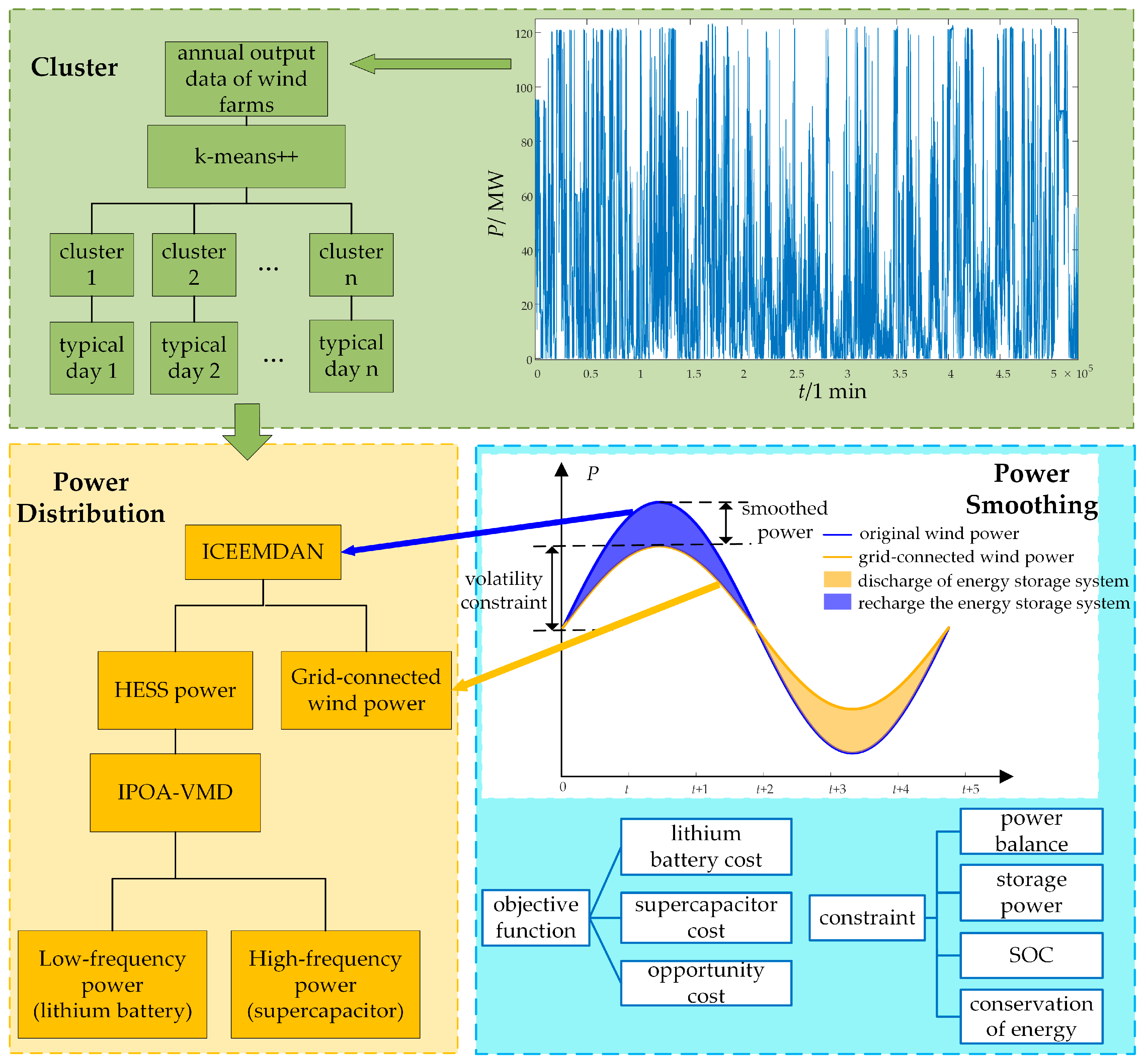
- A novel method for selecting typical daily wind farm output based on an improved k-means is proposed. This method optimizes initial centroids using k-means++ and determines the optimal number of clusters through the silhouette coefficient (SC) and the Davies–Bouldin index (DBI). A typical-day selection mechanism is established based on cluster centroid distances and cumulative fluctuation magnitudes, overcoming the limitation of traditional methods that rely solely on mean values to select representative scenarios, making the selected typical days more suitable for wind power fluctuation smoothing.
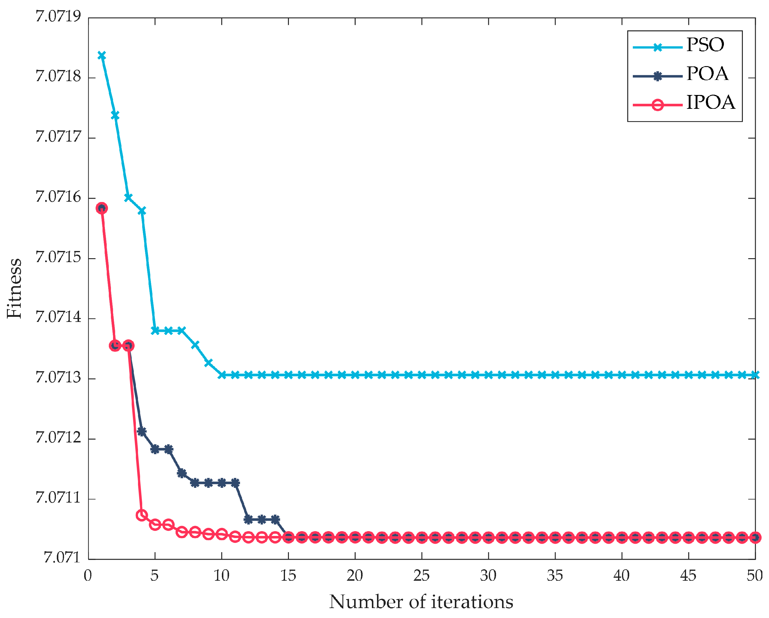
- A power allocation strategy based on ICEEMDAN and IPOA-VMD is proposed. Compared with conventional PSO and POA, IPOA demonstrated superior search speed and optimization accuracy, enhancing the mode-matching accuracy of VMD. By leveraging the coordinated compensation of supercapacitors and lithium batteries, the proposed strategy reduced the occurrences of grid power fluctuation exceeding limits to zero at both 1 min and 10 min time scales, significantly improving wind power fluctuation smoothing and optimizing the overall performance of the HESS.
- A HESS capacity optimization model based on typical daily data was developed. Case study analysis showed that, compared with conventional strategies, the proposed approach increased the wind power fluctuation qualification rate to 100% while reducing the annualized cost of the HESS by 7.79%, providing valuable engineering insights for HESS capacity planning.
2. Methodology
2.1. Method for Selecting Typical Days of Wind Power Based on k-means++
2.1.1. k-means++ Clustering Algorithm
- Randomly select a sample point from the dataset as the initial cluster center c.
- Calculate the shortest Euclidean distance between each sample point and the existing cluster centers, denoted as d(x).
- Calculate the probability of each sample being selected as the next cluster center, , and use the roulette method to choose the next cluster center.
- Repeat steps 2 and 3 until k cluster centers are selected.
- For each sample in the dataset, calculate the Euclidean distance to the k cluster centers, and assign it to the class corresponding to the closest cluster center.
- For each class, recalculate its cluster center.
- Repeat steps 5 and 6 until the cluster centers no longer change.
2.1.2. Selection of the Optimal Number of Clusters
2.1.3. Rules for Selecting Typical Days
- Compute the Euclidean distance di of each sample zi from its cluster centroid ci and the cumulative fluctuations Bi of sample zi. Here, the fluctuations are defined as the differences between consecutive one-minute power datapoints, and the value of cumulative fluctuations is the sum of all fluctuations over a day.
- Normalize the Euclidean distance di and cumulative fluctuations Bi for each sample, introducing a weight coefficient γ (0 < γ < 1).
- Calculate the comprehensive weight wi for each sample as , where and are the maximum Euclidean distance and maximum cumulative fluctuations among all samples, respectively.
- Select the sample with the smallest comprehensive weight wi in each cluster as the typical day data for that cluster.
2.2. Power Distribution Strategy
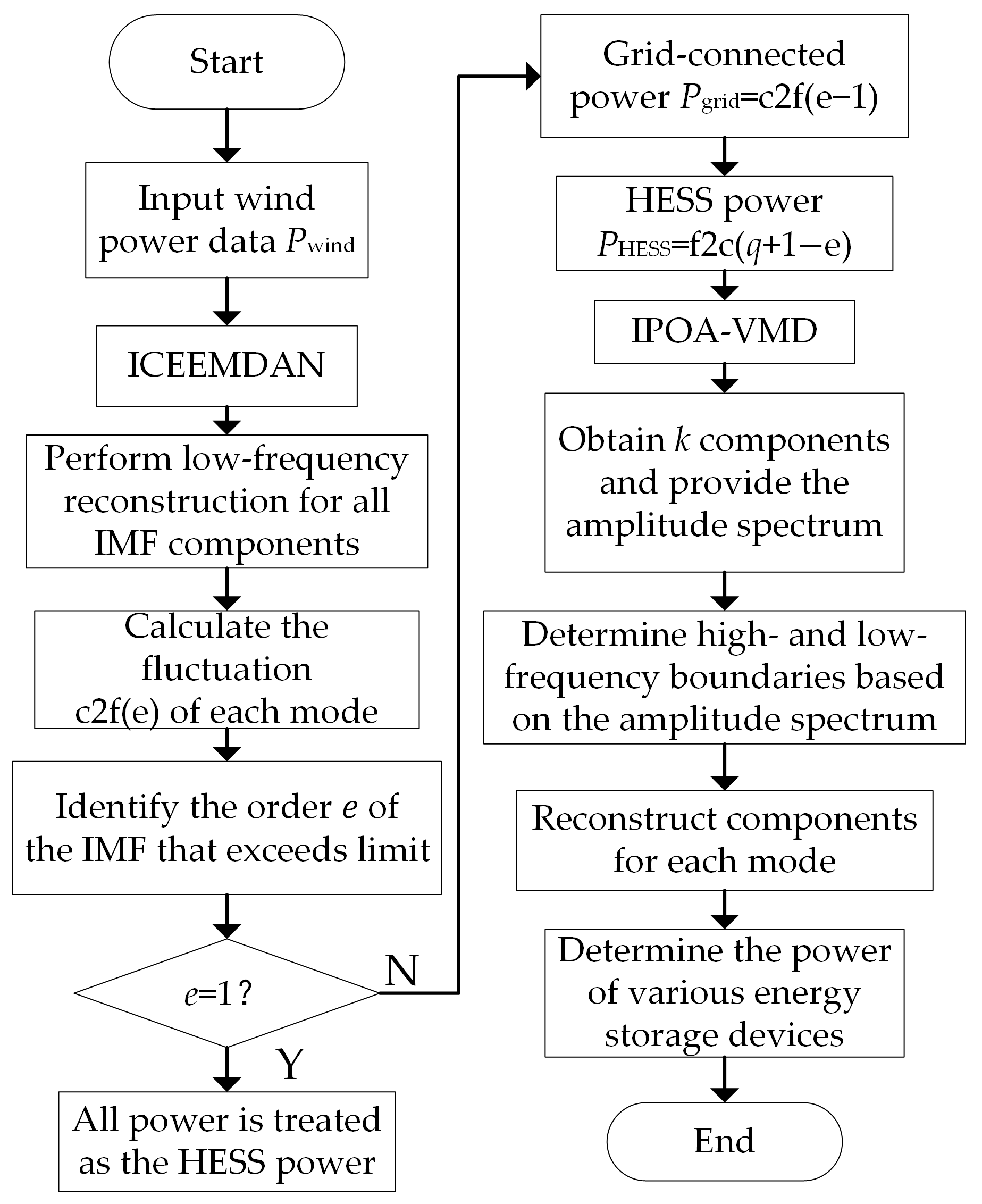
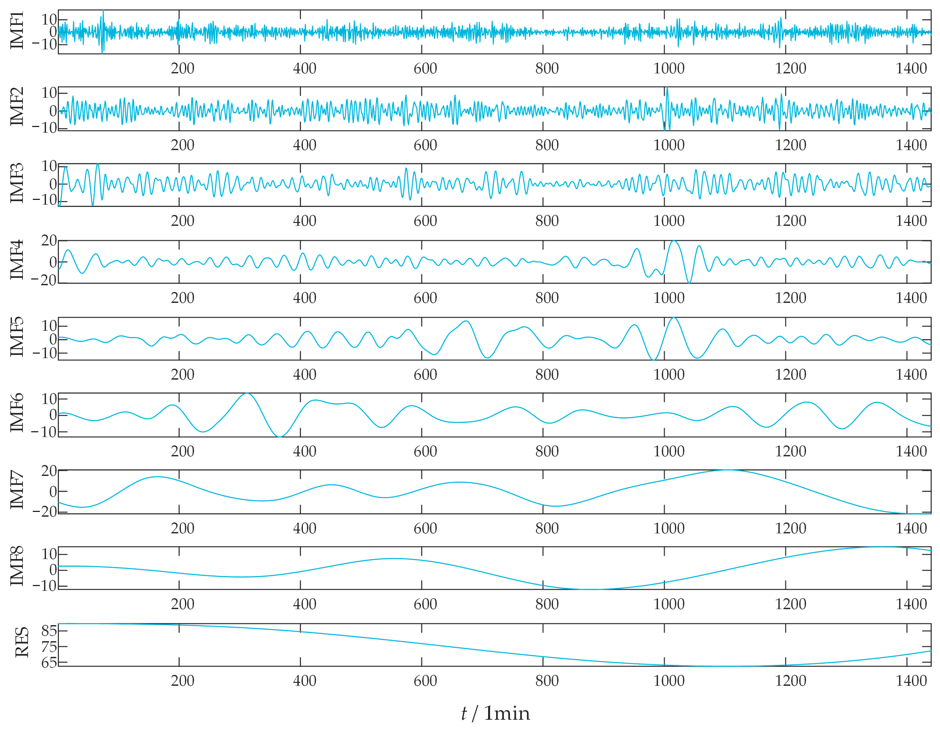
2.2.1. ICEEMDAN
- Add i groups of white noise W(i) to the original wind speed series, resulting in:
- 2.
- Calculate the envelope and obtain the first residual component and the first modal component by averaging:
- 3.
- Continue adding white noise and use local mean decomposition to calculate the q-th order residual and the q-th order modal component:
- 4.
- Continue until the decomposition is completed, obtaining all the modes and residuals.
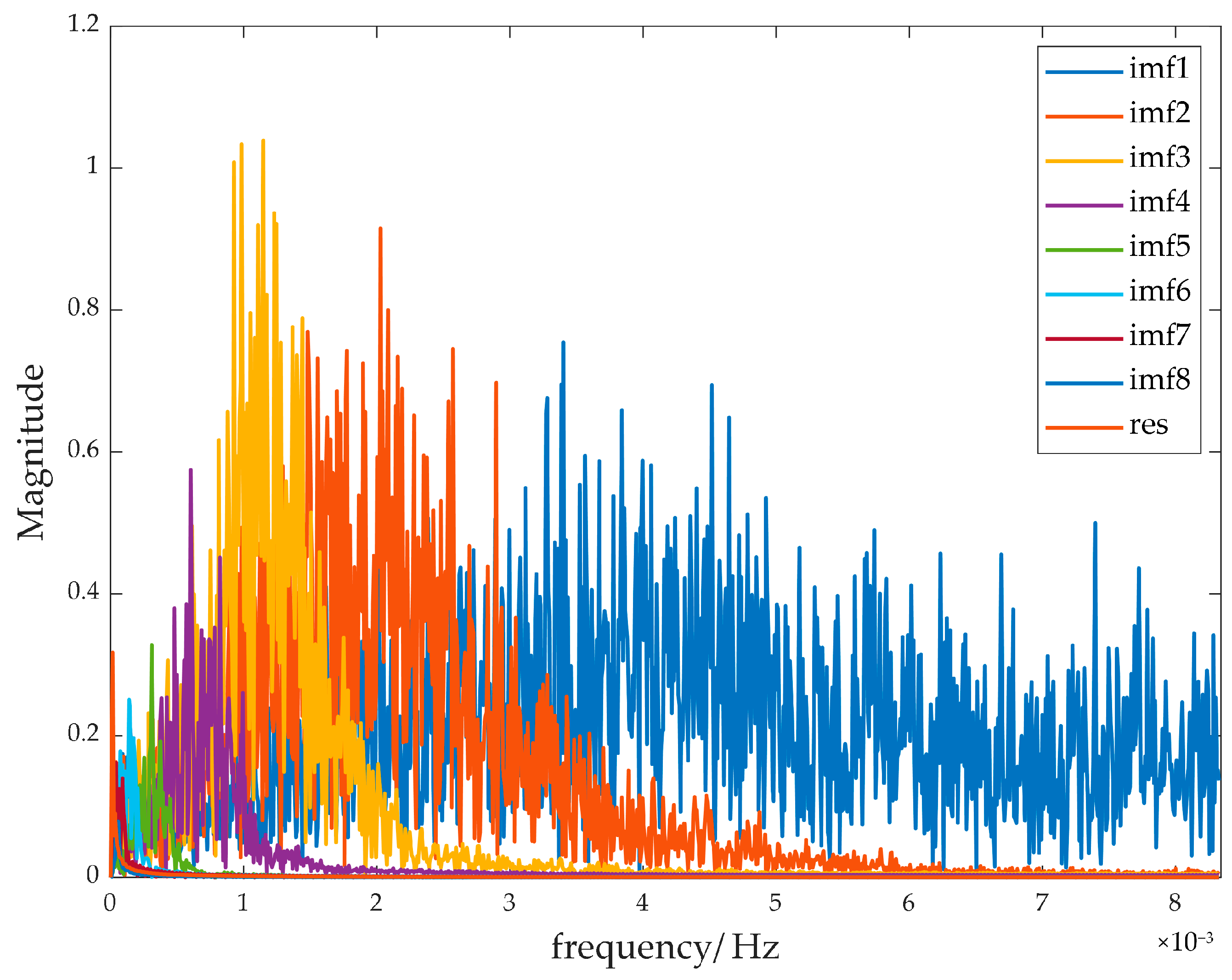
2.2.2. IPOA-VMD
- Construct the variational problem. By applying the Hilbert transform to the input signal, the corresponding analytic signal is obtained. Multiplying it by the corresponding center frequency shifts the spectrum to the base frequency band, and Gaussian smoothing is used to adjust the bandwidth of the signal. The constrained variational model is:
- 2.
- Reconstruct the constrained problem. To solve the above problem, a quadratic penalty term is used to penalize the violation of the constraints, transforming the constrained problem into an unconstrained problem. The augmented Lagrange function operator λ and the penalty factor α are introduced to complete the reconstruction of the problem, which is represented as:
- 3.
- Solve the unconstrained problem. The optimal solution of the problem is searched through a frequency-domain iterative method. Using the alternating direction method of multipliers, the components uk(t), center frequencies ωk, and Lagrange multipliers are iteratively updated until the stopping conditions are met. The update process and iteration stopping expressions are shown in Equations (11) and (12).
- Logistic chaotic mapping strategy [26]
- 2.
- Development stage position optimization based on Lévy flight
2.2.3. Power Distribution Strategy Based on Two-Stage Decomposition
2.3. HESS Capacity Optimization Configuration
2.3.1. Objective Function
- Investment Cost:
- 2.
- O&M Cost:
- 3.
- Residual Value:
- 4.
- Wind Power Fluctuation Opportunity Compensation Cost:
2.3.2. Constraints
- Power balance constraint
- 2.
- Charge–discharge power constraint
- 3.
- Energy conservation constraint
- 4.
- SOC constraint
3. Discussion and Analysis of Experimental Results
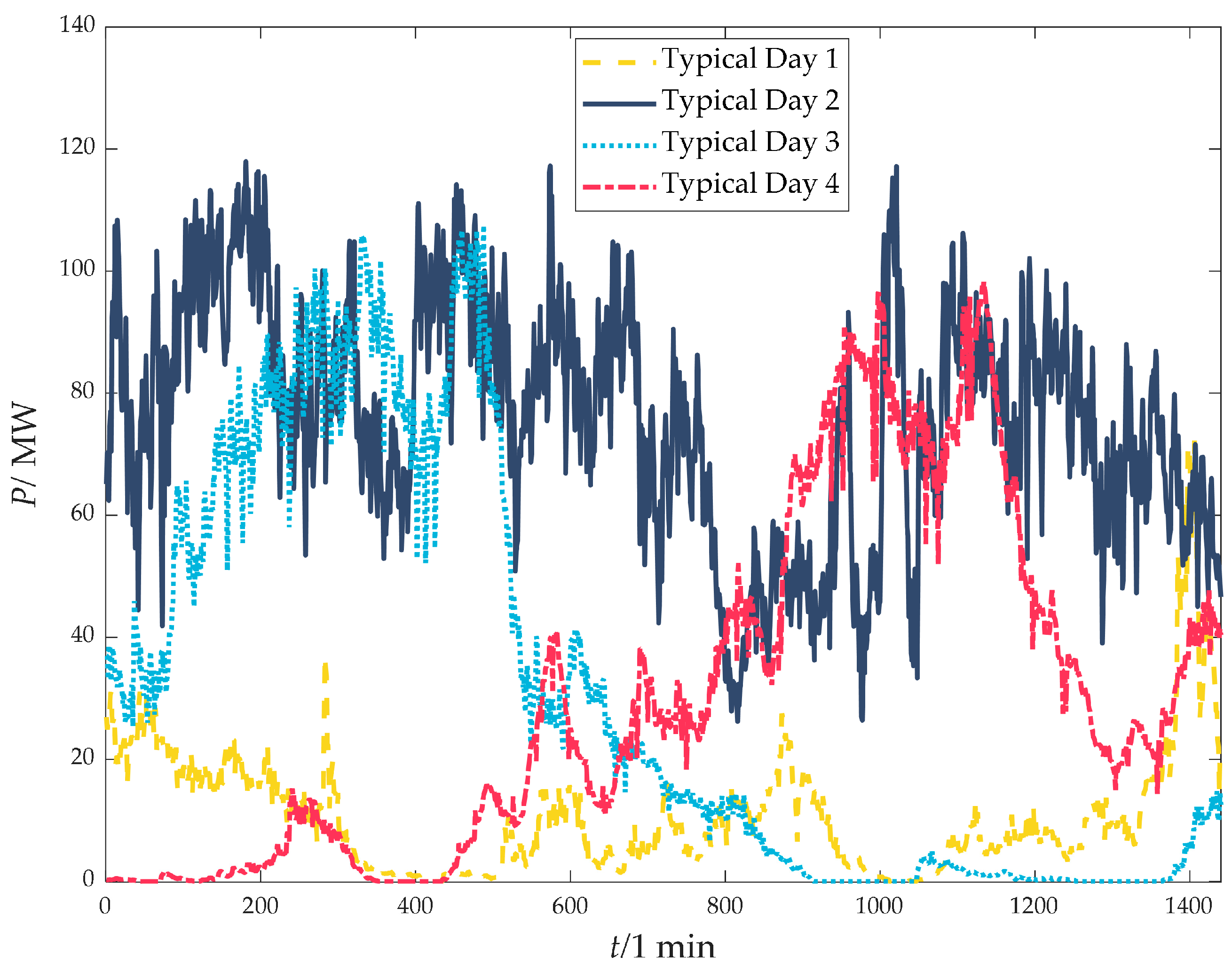
3.1. Clustering to Generate Typical Days
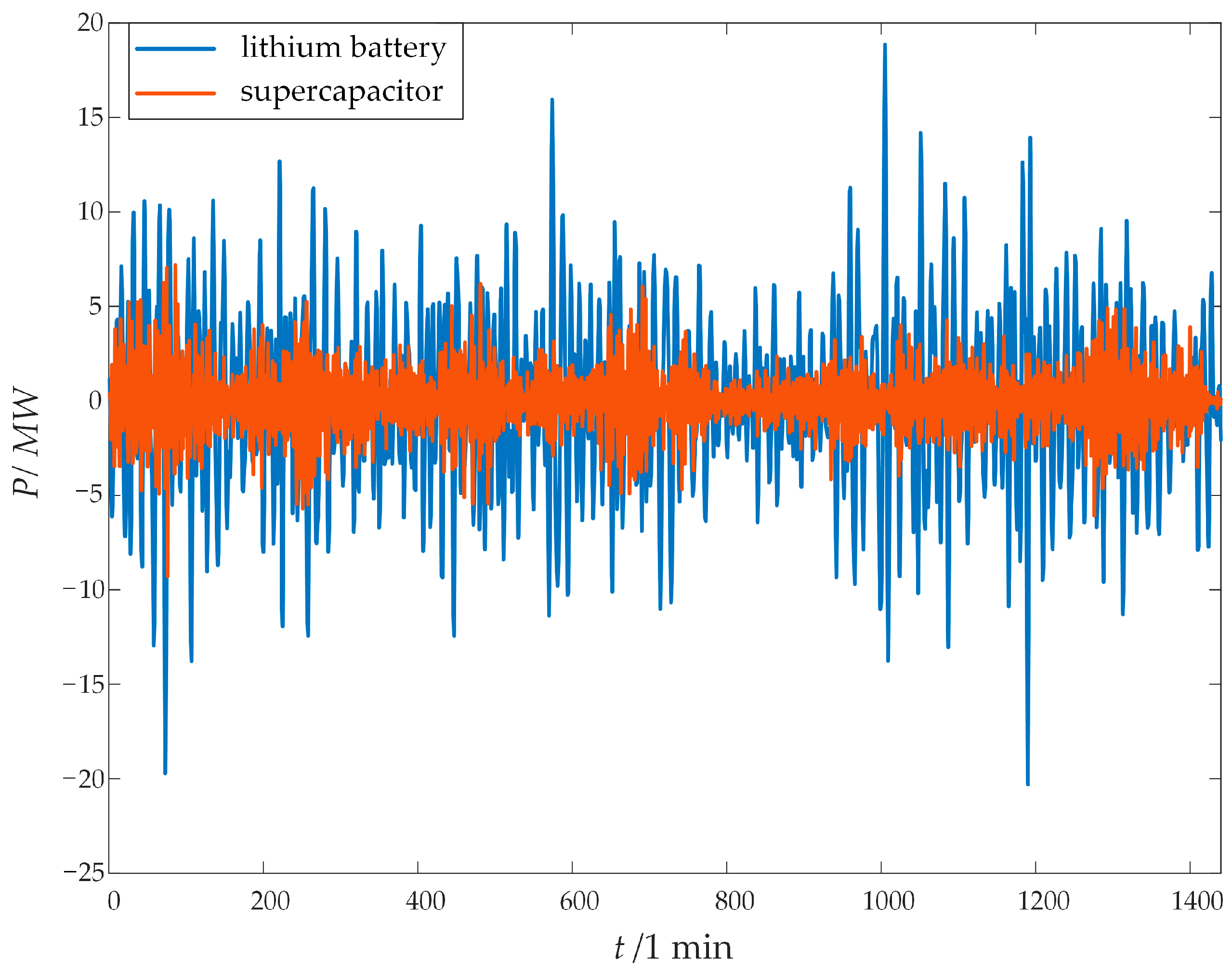
3.2. Power Distribution
3.3. Results of HESS Capacity Optimization Configuration
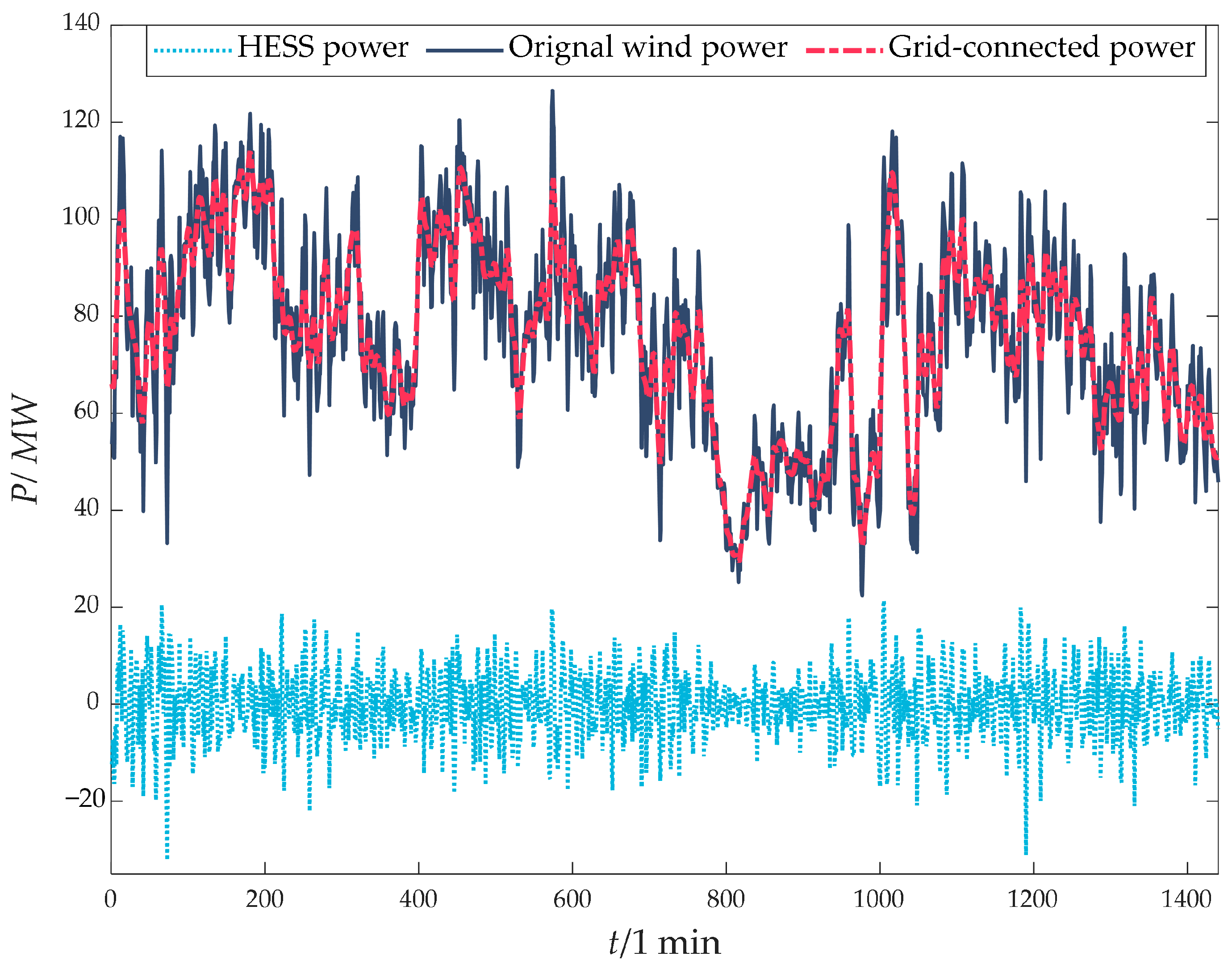
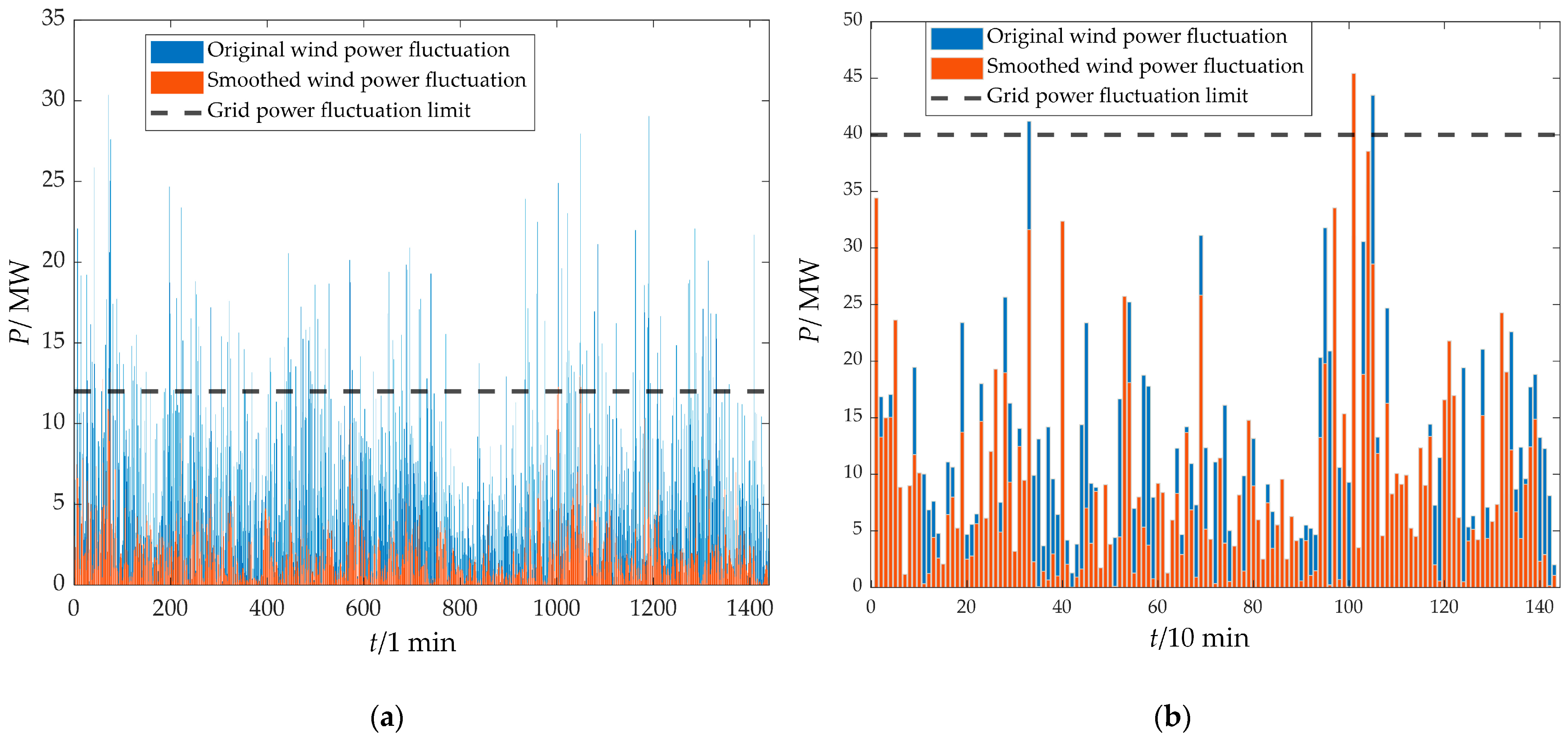
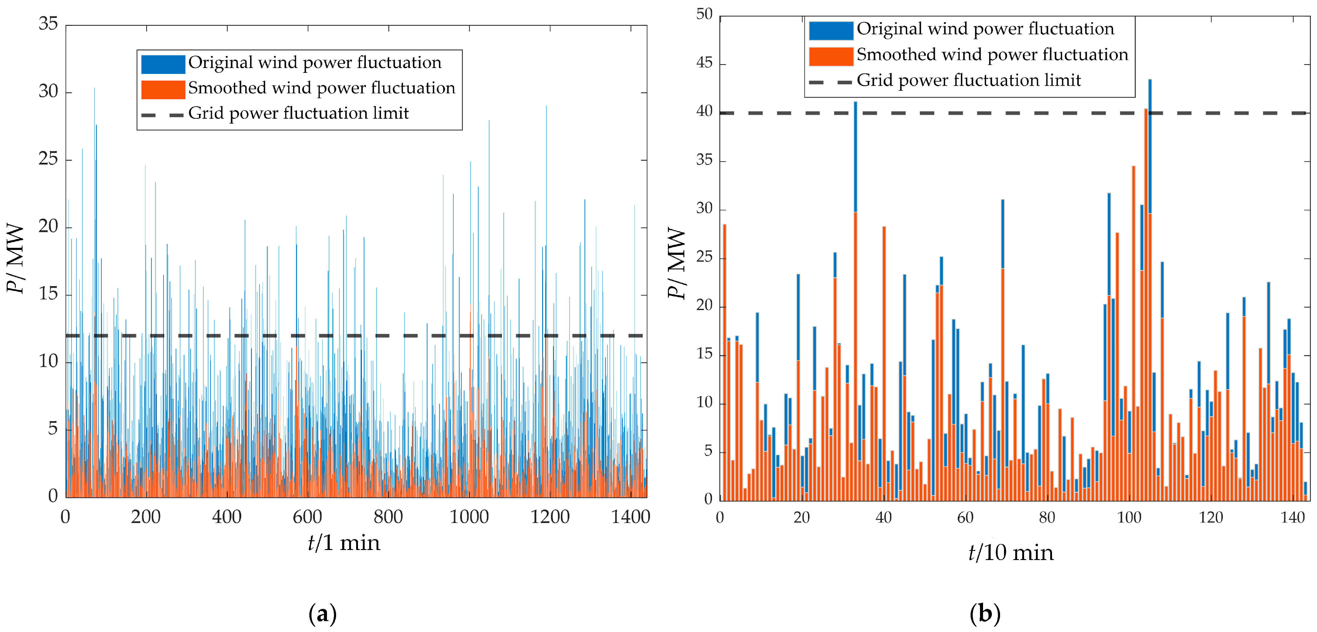
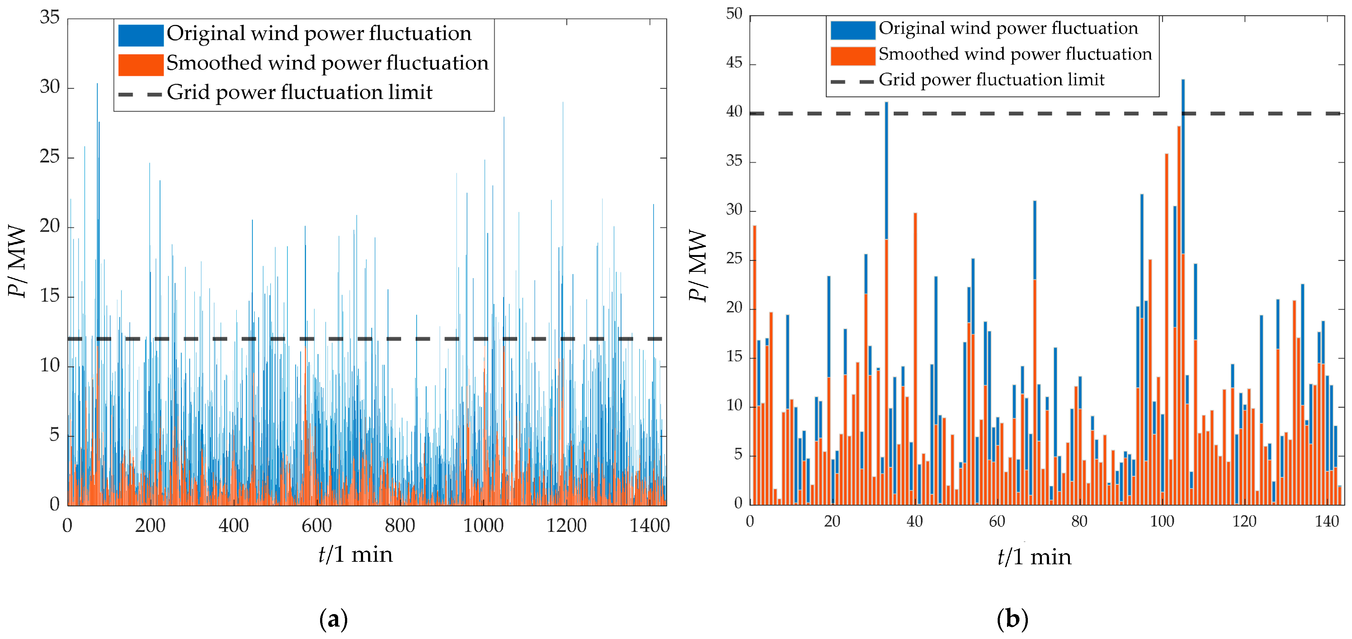
3.4. Analysis of Wind Power Smoothing Effect
4. Conclusions
- Compared with traditional PSO and POA, the IPOA was used to optimize the modal number K and quadratic penalty factor α for VMD, performing better in terms of search speed and optimization accuracy. It effectively improved the modal matching accuracy of VMD, enhancing the accuracy of internal power distribution in the HESS.
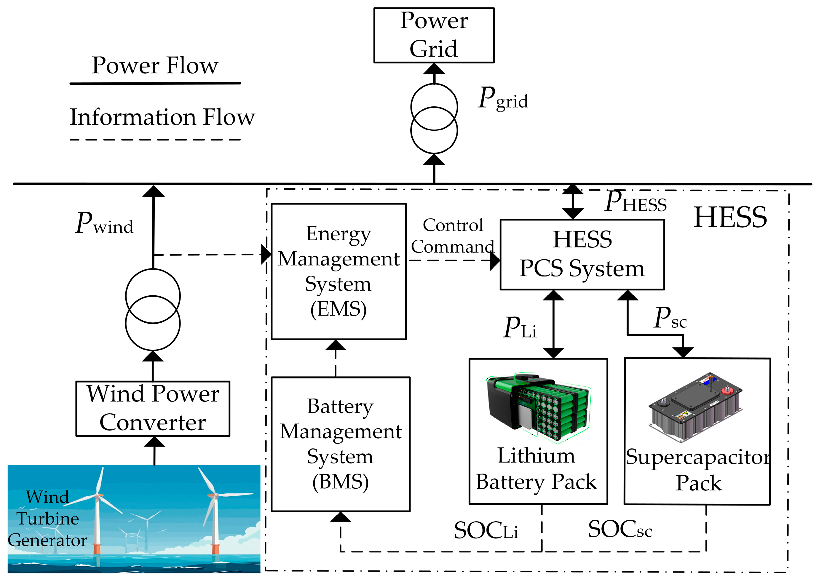
- The two-stage decomposition power distribution strategy based on ICEEMDAN and IPOA-VMD could effectively smooth wind power fluctuations, fully utilizing the advantages of power-type and energy-type storage and achieving precise separation of high-frequency and low-frequency components. Through the collaborative compensation of supercapacitors and lithium batteries, the proposed strategy reduced the number of grid-connected power fluctuation exceedances to 0 on both the 1 min and 10 min time scales, improving the wind power fluctuation smoothing effect and optimizing the overall performance of the HESS.
- k-means++ was used to cluster the annual wind power data by combining SC and DBI, and typical-day data were determined based on the overall characteristics and cumulative fluctuation of each clustering scenario. The case study was conducted based on this, and the results showed that the proposed strategy not only met the grid-connected power fluctuation requirements of wind farms but reduced the overall HESS cost by 7.79% compared with traditional strategies, providing an engineering reference value for HESS capacity planning.
- The HESS capacity optimization model for smoothing wind power fluctuations established in this study does not consider the impact of dynamic electricity prices and ancillary service revenues on the economic viability of the HESS. Future research is planned involving developing a multiobjective optimization model incorporating demand response and ancillary services to quantify the added value of energy storage participation in the market and further improve the full lifecycle economic analysis.
Author Contributions
Funding
Data Availability Statement
Conflicts of Interest
Appendix A

| Parameter | Npop | Nmax | Kb | αb | tau | DC | init | tol |
|---|---|---|---|---|---|---|---|---|
| Value | 20 | 70 | [1, 10] | [10, 10,000] | 0 | 0 | 1 | 1 × 10⁻⁶ |
| Category | Parameter Item | Configuration Value/Description |
|---|---|---|
| YALMIP | Version | 20180612 |
| Optimization Model | optimizer function | |
| Solving Precision | sdpsettings(’solver’,’gurobi+’,’verbose’,2) | |
| Constraint Tolerance | 1 × 10⁻⁶ | |
| Gurobi | Version | 10.0.1 |
| MIPGap | 0.01 | |
| Maximum Computation Time | 3600 s |
| Parameter Name | Value |
|---|---|
| Unit capacity cost of lithium batteries /[10 k CNY·(MW·h)−1] | 100 |
| Unit power cost of lithium batteries /[10 k CNY·(MW)−1] | 150 |
| Unit capacity cost of supercapacitors /[10 k CNY·(MW·h)−1] | 600 |
| Unit power cost of supercapacitors /[10 k CNY·(MW)−1] | 100 |
| SOC limit of lithium batteries | [0.2, 0.8] |
| SOC limit of supercapacitors | [0.1, 0.9] |
| Discount rate r | 5% |
| Operating lifespan of lithium batteries YLi/year | 5 |
| Operating lifespan of supercapacitors Ysc/year | 15 |
| Proportion of O&M costs to investment costs for lithium batteries aLi | 2% |
| Proportion of O&M costs to investment costs for supercapacitors asc | 2% |
| Residual value rate of lithium batteries bLi | 10% |
| Residual value rate of supercapacitors bsc | 20% |
| Opportunity compensation cost coefficient /[10 k CNY·(MW·h)−1] | 0.32 |
References
- Roga, S.; Bardhan, S.; Kumar, Y.; Dubey, S.K. Recent technology and challenges of wind energy generation: A review. Sustain. Energy Technol. Assess. 2022, 52, 102239. [Google Scholar] [CrossRef]
- Deguenon, L.; Yamegueu, D.; Gomna, A. Overcoming the challenges of integrating variable renewable energy to the grid: A comprehensive review of electrochemical battery storage systems. J. Power Sources 2023, 580, 233343. [Google Scholar] [CrossRef]
- Cui, D.; Jin, Y.; Wang, Y.; Yuan, Z.; Cai, G.; Liu, C.; Ge, W. Combined thermal power and battery low carbon scheduling method based on variational mode decomposition. Int. J. Electr. Power Energy Syst. 2023, 145, 108644. [Google Scholar] [CrossRef]
- Lei, S.; He, Y.; Zhang, J.; Deng, K. Optimal configuration of hybrid energy storage capacity in a microgrid based on variational mode decomposition. Energies 2023, 16, 4307. [Google Scholar] [CrossRef]
- Xinghao, P.; Yanting, L. Wind Power Scenario Generation Method and Application Based onSpatiotemporal Covariance Function. J. Shanghai Jiaotong Univ. 2023, 57, 1531. [Google Scholar]
- Fei, Z.; Yang, H.; Du, L.; Guerrero, J.M.; Meng, K.; Li, Z. Two-stage coordinated operation of A green multi-energy ship microgrid with underwater radiated noise by distributed stochastic approach. IEEE Trans. Smart Grid 2024. [Google Scholar] [CrossRef]
- Yang, Z.; Ren, Z.; Li, H.; Sun, Z.; Feng, J.; Xia, W. A multi-stage stochastic dispatching method for electricity-hydrogen integrated energy systems driven by model and data. Appl. Energy 2024, 371, 123668. [Google Scholar] [CrossRef]
- Wang, Y.; Liu, Y.; Kirschen, D.S. Scenario reduction with submodular optimization. IEEE Trans. Power Syst. 2016, 32, 2479–2480. [Google Scholar] [CrossRef]
- Wu, A. Capacity Optimization Configuration of Energy Storage System in Wind Farm Based on Sand Cat Swarm Algorithm. In Proceedings of the 2023 Asia Conference on Power, Energy Engineering and Computer Technology (PEECT), Qingdao, China, 21–23 July 2023; pp. 12–17. [Google Scholar]
- Tiejiang, Y.; Yang, Y.; Rui, L.; Dongfang, J. Optimized Configuration of Hydrogen-Energy Microgrid Capacity Considering Source Charge Uncertainties. Electr. Power 2023, 56, 21–32. [Google Scholar]
- Zhang, Y.; Pan, G.; Chen, B.; Han, J.; Zhao, Y.; Zhang, C. Short-term wind speed prediction model based on GA-ANN improved by VMD. Renew. Energy 2020, 156, 1373–1388. [Google Scholar] [CrossRef]
- Lixiang, H.; Xinyan, Z.; Shuai, L.; Rui, S.; Shiqiang, L.; Guanghao, Z. Hybrid Energy Storage Power Distribution Strategy for Smoothing Wind-Photovoltaic Power Fluctuation. Sci. Technol. Eng. 2023, 23, 10825–10834. [Google Scholar]
- Long, C.; Fanghua, Z. Wavelet Transform Method for Hybrid Energy Storage System Smoothing Power Fluctuation. Electr. Power Autom. Equip./Dianli Zidonghua Shebei 2021, 41, 100–104+128. [Google Scholar]
- Kunhua, J.; Yun, W.; Lina, D.; Yao, Z. Hybrid Energy Storage Wind Power Smoothing Control Strategy for Improving Bidirectional Regulation Ability. Smart Power 2024, 52, 55–62. [Google Scholar]
- Ren, Y.; Suganthan, P.N.; Srikanth, N. A comparative study of empirical mode decomposition-based short-term wind speed forecasting methods. IEEE Trans. Sustain. Energy 2014, 6, 236–244. [Google Scholar] [CrossRef]
- Lin, L.; Zhu, L.; Yang, R.; Gao, Y.; Wu, Q. Capacity optimization of hybrid energy storage for smoothing power fluctuations based on spectrum analysis. In Proceedings of the 2017 2nd International Conference on Power and Renewable Energy (ICPRE), Chengdu, China, 20–23 September 2017; pp. 61–65. [Google Scholar]
- Qing, Z.; Xinran, L.; Ming, Y.; Yijia, C.; Peiqiang, L. Capacity Determination of Hybrid Energy Storage System for Smoothing Wind Power Fluctuations with Maximum Net Benefit. Trans. China Electrotech. Soc. 2016, 31, 40–48. [Google Scholar]
- Zhang, Y.; Zhao, F. Optimal configuration of wind storage capacity based on VMD and improved GWO. J. Phys. Conf. Ser. 2022, 2378, 012048. [Google Scholar] [CrossRef]
- Zhang, Y.; Pan, Z.; Wang, H.; Wang, J.; Zhao, Z.; Wang, F. Achieving wind power and photovoltaic power prediction: An intelligent prediction system based on a deep learning approach. Energy 2023, 283, 129005. [Google Scholar] [CrossRef]
- Arthur, D.; Vassilvitskii, S. k-means++: The Advantages of Careful Seeding; Stanford: Palo Alto, CA, USA, 2006. [Google Scholar]
- Miraftabzadeh, S.M.; Colombo, C.G.; Longo, M.; Foiadelli, F. K-means and alternative clustering methods in modern power systems. IEEE Access 2023, 11, 119596. [Google Scholar] [CrossRef]
- Maulik, U.; Bandyopadhyay, S. Performance evaluation of some clustering algorithms and validity indices. IEEE Trans. Pattern Anal. Mach. Intell. 2002, 24, 1650–1654. [Google Scholar] [CrossRef]
- Poongadan, S.; Lineesh, M. Non-linear Time Series Prediction using Improved CEEMDAN, SVD and LSTM. Neural Process. Lett. 2024, 56, 164. [Google Scholar] [CrossRef]
- Dragomiretskiy, K.; Zosso, D. Variational mode decomposition. IEEE Trans. Signal Process. 2013, 62, 531–544. [Google Scholar] [CrossRef]
- Trojovský, P.; Dehghani, M. Pelican optimization algorithm: A novel nature-inspired algorithm for engineering applications. Sensors 2022, 22, 855. [Google Scholar] [CrossRef]
- Pareek, N.K.; Patidar, V.; Sud, K.K. Image encryption using chaotic logistic map. Image Vis. Comput. 2006, 24, 926–934. [Google Scholar] [CrossRef]
- Jin, Z.; He, D.; Wei, Z. Intelligent fault diagnosis of train axle box bearing based on parameter optimization VMD and improved DBN. Eng. Appl. Artif. Intell. 2022, 110, 104713. [Google Scholar] [CrossRef]
- Li, Z.; Zhao, H.; Lin, Y. Multi-task convolutional neural network with coarse-to-fine knowledge transfer for long-tailed classification. Inf. Sci. 2022, 608, 900–916. [Google Scholar] [CrossRef]
- Qu, H.; Ye, Z. Comparison of Dynamic Response Characteristics of Typical Energy Storage Technologies for Suppressing Wind Power Fluctuation. Sustainability 2023, 15, 2437. [Google Scholar] [CrossRef]
- Xiong, X.; Rengang, Y.; Lin, Y.; Jianlin, L. Economic Evaluation of Large-Scale Energy Storage Allocation in Power Demand Side. Trans. China Electrotech. Soc. 2013, 28, 224–230. [Google Scholar]
- Suhua, L.; Tianmeng, Y.; Yaowu, W.; Yongcan, W. Coordinated Optimal Operation of Hybrid Energy Storage in Power System Accommodated High Penetration of Wind Power. Autom. Electr. Power Syst. 2016, 40, 30–35. [Google Scholar]


| Country | Wind Power Grid Integration Standards |
|---|---|
| United States | The 1 min ramp-up rate is less than 10% of the installed capacity |
| Canada | The 1 min ramp-up rate is less than 10% of the installed capacity |
| Denmark | The 1 min ramp-up rate is less than 5% of the installed capacity |
| Germany | At startup, the 1 min ramp-up rate is less than 10% of the installed capacity |
| United Kingdom | The 1 min variation is less than 10 MW, and the 1 min average ramp-up rate must not exceed three times the 10 min average ramp-up rate |
| China | Installed capacity < 30 MW: Variation within 10 min is less than 10 MW, and variation within 1 min is less than 3 MW Installed capacity 30–150 MW: Variation within 10 min is less than 1/3, and variation within 1 min is less than 1/10 Installed capacity > 150 MW: Variation within 10 min is less than 50 MW, and variation within 1 min is less than 15 MW |
| Clustering Algorithm | k = 3 | k = 4 | k = 5 | k = 6 | k = 7 |
|---|---|---|---|---|---|
| k-means | 0.5824 | 0.3894 | 0.3941 | 0.3892 | 0.3708 |
| k-means++ | 0.5800 | 0.6083 | 0.3864 | 0.3995 | 0.3904 |
| HC | 0.5858 | 0.5972 | 0.3829 | 0.3790 | 0.3892 |
| FCM | 0.4842 | 0.3852 | 0.3120 | 0.3147 | 0.2293 |
| Clustering Algorithm | k = 3 | k = 4 | k = 5 | k = 6 | k = 7 |
|---|---|---|---|---|---|
| k-means | 1.2126 | 1.4144 | 1.3399 | 1.4631 | 1.5443 |
| k-means++ | 1.2131 | 1.1435 | 1.3176 | 1.4487 | 1.5250 |
| HC | 1.3013 | 1.3178 | 1.3314 | 1.5222 | 1.5166 |
| FCM | 1.2948 | 1.4562 | 2.0640 | 1.8110 | 1.9965 |
| Parameters | Scheme 1 | Scheme 2 | Scheme 3 | Scheme 4 |
|---|---|---|---|---|
| Lithium battery power /MW | 10.61761 | 7.476901 | 6.034713 | 7.361035 |
| Lithium battery capacity/MW·h | 0.5705331 | 1.382324 | 0.3252731 | 1.002809 |
| Supercapacitor power/MW | 5.513871 | 4.450731 | 3.938104 | 4.923756 |
| Supercapacitor capacity/MW·h | 0.123192 | 0.1467984 | 0.09366347 | 0.1449318 |
| Investment cost/10 k CNY | 606.0136 | 477.9401 | 357.9292 | 461.9565 |
| O&M cost/10 k CNY | 1.212027 | 9.558803 | 7.158584 | 9.516771 |
| Recovery value/10 k CNY | 49.07465 | 39.34212 | 29.18946 | 37.54483 |
| Opportunity compensation cost/10 k CNY | 123.6268 | 227.6628 | 319.11602 | 205.0725 |
| Annualized total cost/10 k CNY | 692.6860 | 682.9033 | 655.0143 | 638.7233 |
| Typical Day | ELi | PLi | Esc | Psc |
|---|---|---|---|---|
| 1 | 0.3553705 | 3.059701 | 0.04220754 | 1.502692 |
| 2 | 1.002809 | 7.361035 | 0.1449318 | 4.923756 |
| 3 | 0.3836545 | 7.436658 | 0.06125014 | 3.171559 |
| 4 | 0.2594061 | 4.601879 | 0.03802841 | 1.835683 |
| Final configuration results | 1.002809 | 7.436658 | 0.1449318 | 4.923756 |
Disclaimer/Publisher’s Note: The statements, opinions and data contained in all publications are solely those of the individual author(s) and contributor(s) and not of MDPI and/or the editor(s). MDPI and/or the editor(s) disclaim responsibility for any injury to people or property resulting from any ideas, methods, instructions or products referred to in the content. |
© 2025 by the authors. Licensee MDPI, Basel, Switzerland. This article is an open access article distributed under the terms and conditions of the Creative Commons Attribution (CC BY) license (https://creativecommons.org/licenses/by/4.0/).
Share and Cite
Zhang, X.; Kang, L.; Wang, X.; Liu, Y.; Huang, S. Capacity Optimization Configuration of Hybrid Energy Storage Systems for Wind Farms Based on Improved k-means and Two-Stage Decomposition. Energies 2025, 18, 795. https://doi.org/10.3390/en18040795
Zhang X, Kang L, Wang X, Liu Y, Huang S. Capacity Optimization Configuration of Hybrid Energy Storage Systems for Wind Farms Based on Improved k-means and Two-Stage Decomposition. Energies. 2025; 18(4):795. https://doi.org/10.3390/en18040795
Chicago/Turabian StyleZhang, Xi, Longyun Kang, Xuemei Wang, Yangbo Liu, and Sheng Huang. 2025. "Capacity Optimization Configuration of Hybrid Energy Storage Systems for Wind Farms Based on Improved k-means and Two-Stage Decomposition" Energies 18, no. 4: 795. https://doi.org/10.3390/en18040795
APA StyleZhang, X., Kang, L., Wang, X., Liu, Y., & Huang, S. (2025). Capacity Optimization Configuration of Hybrid Energy Storage Systems for Wind Farms Based on Improved k-means and Two-Stage Decomposition. Energies, 18(4), 795. https://doi.org/10.3390/en18040795