Multi-Timescale Voltage Control Method Using Limited Measurable Information with Explainable Deep Reinforcement Learning

Abstract

The integration of photovoltaic (PV) power generation systems has significantly increased the complexity of voltage distribution in power grids, making it challenging for conventional Load Ratio Control Transformers (LRTs) to manage voltage fluctuations caused by weather-dependent PV output variations. Power Conditioning Systems (PCSs) interconnected with PV installations are increasingly considered for voltage control to address these challenges. This study proposes a Machine Learning (ML)-based control method for sub-transmission grids, integrating long-term LRT tap-changing with short-term reactive power control of PCSs. The approach estimates the voltage at each grid node using a Deep Neural Network (DNN) that processes measurable substation data. Based on these estimated voltages, the method determines optimal LRT tap positions and PCS reactive power outputs using Deep Reinforcement Learning (DRL). This enables real-time voltage monitoring and control using only substation measurements, even in grids without extensive sensor installations, ensuring all node voltages remain within specified limits. To improve the model’s transparency, Shapley Additive Explanation (SHAP), an Explainable AI (XAI) technique, is applied to the DRL model. SHAP enhances interpretability and confirms the effectiveness of the proposed method. Numerical simulations further validate its performance, demonstrating its potential for effective voltage management in modern power grids.

1. Introduction

In recent years, Renewable Energy Sources (RESs) have gained worldwide attention due to environmental concerns, leading to significant progress in the development of Distributed Energy Resources (DERs) in power grids. Among these, photovoltaic (PV) power generation systems, a representative of RESs, are experiencing a period of rapid growth [1]. PV systems are installed in not only a relatively small-scale source, such as roof-top PV connected to distribution grids, but also large-scale plants in sub-transmission girds to reduce costs and improve generation efficiency [2,3]. Massive PV interconnection leads to voltage rises due to reverse power flow and fast voltage fluctuations caused by changing weather conditions, complicating the maintenance of proper voltage ranges [4]. Furthermore, increased reverse power flow can cause not only voltage rises, but also voltage drops in the grid [5]. Consequently, the voltage distribution becomes significantly more complex with the introduction of PV systems.

Conventional voltage control in sub-transmission grids typically relies on devices such as Load Ratio Control Transformers (LRTs) and Static Capacitors (SCs). However, the mechanical operation of these devices slows down the control cycle, and their frequent usage further reduces their operational lifespan. To address these limitations, the reactive power capabilities of Power Conditioning Systems (PCSs) for PV systems have emerged as a promising solution to mitigate voltage fluctuations [6,7]. As a type of power electronics device, PCSs offer the advantage of a very fast response time. Consequently, there has been significant research on reactive power control methods for PCSs. In [8], constant power factor control of the PCS maintained the grid voltages within a proper range in an example grid based on the actual distribution grid in Japan. However, the constant power factor control method cannot handle the voltage fluctuations caused by weather conditions. In [9], each PCS mitigated voltage fluctuations through reactive power compensation according to the volt-var curve. By updating the control parameters of the volt-var curve given to the PCS in real time, the PCSs are able to adapt to disturbances such as weather conditions and voltage changes at the substation. In [10], there is also a global standard for the volt-var curve which is a major control method. However, these methods are local control, not optimal control for the whole grid, and require coordination with LRTs and other control devices with different control cycles. Coordinated control of inverter-based devices, such as PCSs, and mechanical devices, such as LRTs, involves a multi-timescale optimization challenge due to their varying control cycles and characteristics [11,12]. Methods based on Optimal Power Flow (OPF) can maintain proper voltage levels across the grid by improving coordination between multi-timescale devices, including long-term On-Load Tap Changers (OLTCs) or Capacitor Banks (CBs) and short-term inverter-based devices. However, the effectiveness of these methods depends heavily on the accuracy of the grid model and precise forecasts of RES output and load demand, both of which are difficult to achieve [13]. Moreover, recalculating and determining an optimal solution in real time to address rapid PV output fluctuations is a significant challenge, as PV output varies much faster than the time required for optimization computations [13].

Recently, the application of Deep Reinforcement Learning (DRL) to voltage control has gained significant attention as a potential solution to this problem [14]. DRL-based voltage control methods develop optimal control policies by interacting with a grid model during offline training. Once deployed online, the trained DRL agents act as controllers for voltage control devices, making real-time decisions based on observed conditions. Unlike model-based methods, such as those relying on OPF, DRL-based control is a model-free approach that can operate effectively without requiring an accurate grid model during operation [15]. In [16], an Automatic Voltage Control (AVC) method for controlling generator terminal voltage using DRL demonstrated better performance with the Deep Deterministic Policy Gradient (DDPG) algorithm compared to the Deep Q-Network (DQN) algorithm. This highlights that actor–critic DRL methods, such as DDPG, are well suited for continuous-valued control outputs like AVC, as they can directly handle continuous-valued actions. In [17], a safe off-policy DRL algorithm was proposed to minimize the switching costs of slow-timescale discrete devices while maintaining voltage constraints on an hourly basis. Additionally, in [18], a voltage control method using Multi-Agent DDPG (MADDPG) with nine PV inverters was introduced, incorporating cooperation between agents through an attention mechanism.

These voltage control frameworks can be broadly categorized into centralized [16,17] and decentralized control [18]. Decentralized control includes local and distributed control and assumes that communication is possible within a specific area [19]. Because communication costs are lower in decentralized control compared to centralized control, DRL applications have increasingly been explored for multi-timescale voltage control. For example, in [20], a bi-level DRL-based algorithm for multi-timescale voltage control was proposed. The multi-discrete Soft Actor Critic (SAC) algorithm was used to control long-term discrete devices, while the SAC algorithm was used to control short-term continuous devices. However, this approach relied on centralized control for both long-term and short-term devices. In [21], a different multi-timescale voltage control method from [20] was introduced. The proposed method utilized a centralized SAC algorithm for long-term agents with centralized control and a Multi-Agent SAC (MASAC) algorithm for short-term agents with decentralized control. In [22], the concept of multi-timescale voltage control was further advanced, and a framework was proposed to implement the MASAC algorithm for both long-term and short-term control. As outlined above, multi-timescale voltage control has evolved from centralized to decentralized control to minimize communication costs. However, because the OLTC of the substation has the capability to regulate the voltage of entire lower grids connected to it, it relies heavily on grid-wide voltage information [22]. In addition, most decentralized control methods rely on voltage information from the surrounding area.

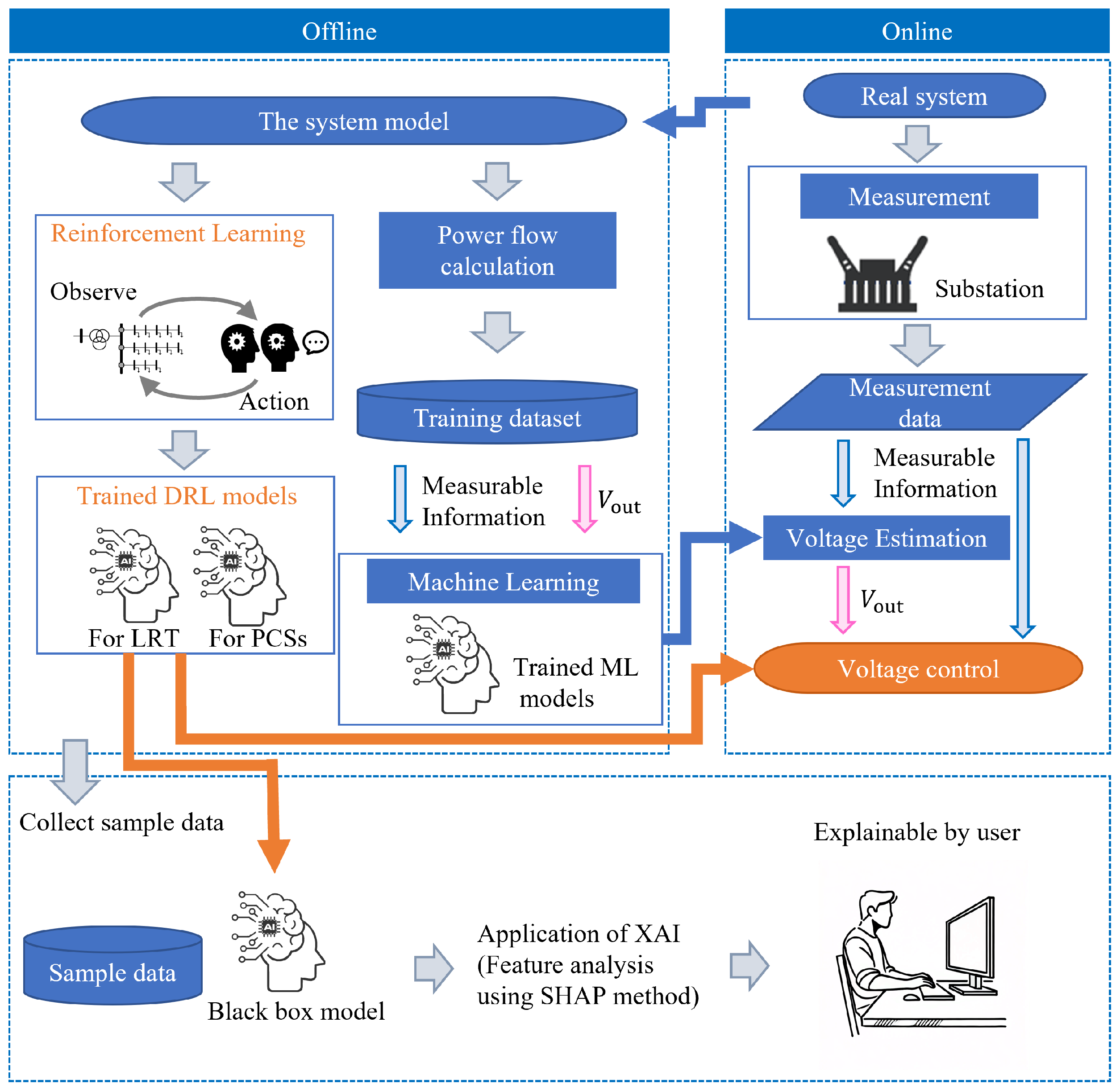
Real-time voltage information is critical for optimal voltage control, as power flow states change dynamically due to load fluctuations, PV output variability, and PCS control. However, acquiring this information in real time incurs high communication costs, even when limited to the surrounding area. To address this challenge, it is essential to develop a framework that further reduces communication costs while enhancing the sophistication of voltage control. To this end, the authors propose a real-time voltage estimation method using Machine Learning (ML) to estimate voltages at all grid nodes based on limited measurable information. Furthermore, the authors also introduce a centralized multi-timescale voltage control method with DRL that uses these real-time estimations for improved performance. This method reduces communication costs while enhancing the sophistication of voltage control. Consequently, developing real-time State Estimation (SE) of the voltage at all nodes using only limited measurable information is essential.

SE in power grids is a critical factor for operational enhancement, and significant research is ongoing in this area. According to the review by [23], most studies focus on modified SE methods aimed at improving data efficiency. However, as noted in [24], it is challenging to use smart meter data as real-time observations for SE because these data update slowly (approximately every 15 min) and often involve delays of up to one day for collection. As a result, real-time measurements in power grids are limited, making real-time SE impossible without the use of pseudo-observations. To address this limitation, various methods have been proposed for generating pseudo-observations for load, including statistical approaches and ML techniques. In [25], a neural network (NN) was employed to enhance the accuracy of load power consumption estimation, which serves as a pseudo-observation value. This approach used three types of information as input: actual load information, weather data, and time information, to predict load power consumptions for the next hour. Research on SE has leveraged ML to accurately estimate pseudo-observations. Building on this, this study aims to estimate voltage as a pseudo-observation value directly and in real-time using ML for real-time voltage control. However, there are few studies on real-time voltage estimation in power grids using only limited real-time information. To address this gap, the authors developed a voltage estimation method using regression trees, a type of ML algorithm, for real-time voltage estimation [26]. This approach uses regression trees to learn the relationship between node voltages (output data) and measurable input data, such as substation secondary-side bus voltage as well as the active and reactive power supplied to each line, which can be obtained in real time at the substation. In [27,28], the authors demonstrated that comprehensive training on assumed PV output and load power data enables accurate voltage estimation under real-time grid conditions. However, previous studies did not consider scenarios where PCS reactive power control for PV systems is implemented. The PCS reactive power output adds complexity to voltage estimation using regression trees. Furthermore, the growing number of PV interconnection points necessitates more accurate voltage estimation while minimizing the size of the training dataset. Recently, Deep Neural Networks (DNNs) have been utilized for estimating pseudo-observations in SE [25] and for power flow calculations [29]. DNNs have gained significant attention due to their effectiveness in addressing highly nonlinear problems. Building on this, this study developed a method for estimating voltages at all grid nodes using DNNs, leveraging real-time information measurable at substations to minimize communication costs. This study further proposed a multi-timescale voltage control method that uses DRL and limited measurable information. In this approach, the estimated voltages serve as input data for the DRL agents. By employing ML-based voltage estimation, the proposed method enables centralized control despite the constraints of limited measurable information. This innovation reduces communication costs while enhancing the sophistication of voltage control. Simulations were then conducted to evaluate the accuracy of the voltage estimation method and to assess the effectiveness of the multi-timescale voltage control with DRL based on the estimated voltages.

DRL-based control faces challenges related to the explainability and transparency of its decision-making processes. The “black box” nature of DRL models can be a significant obstacle to their adoption. To address this issue, Explainable AI (XAI) techniques have been developed in recent years to enhance the interpretability of ML models and make their outputs more understandable. The primary goal of XAI is to enable users to better comprehend the behavior of ML models while maintaining their high performance. The application of XAI in the energy field is quite new, beginning around 2020 [30]. According to [30], the most common XAI techniques in the energy field are Local Interpretable Model-agnostic Explanations (LIMEs) and Shapley Additive Explanations (SHAPs), both of which are compatible with any ML model. In [31], XAI techniques, including Explain Like I’m 5 (ELI5), LIME, and SHAP, were applied to solar power forecasting. Among these, SHAP stands out for its ability to provide both global and local interpretability and is the only method offering a complete explanation of model behavior. In [32], SHAP was also applied to an emergency control scheme for power grids. Few studies in the energy field have explored the interpretability issues of DRLs. However, one notable work [32] implemented SHAP in a DQN model for load shedding. Using SHAP, the average influence of all features on all actions was calculated as a global explanation, while the impact of individual features on specific data points was visualized and evaluated as a local explanation. However, the outputs of the DQN are Q-values, and actions are selected based on the relative evaluation of these Q-values. Despite this, a detailed analysis considering this fact is lacking. Furthermore, there is limited research on applications of the actor–critic method, which is a major DRL algorithm. The interpretability of actor–critic DRL methods should be explored, as the network structure of actor–critic differs from that of Q-learning DRL methods such as DQN. Additionally, there is sufficient scope to discuss the comparison of action decision criteria with other control methods using SHAP. There are also few examples of SHAP being applied in the field of voltage control, making it crucial to clarify the criteria for action decisions in this field. Therefore, the authors applied the SHAP method to multi-timescale voltage control using DRL and conducted a detailed analysis to elucidate the criteria for action decisions in voltage control. Moreover, the SHAP method reveals how the estimated voltage affects the criteria for action decisions in voltage control.

This study proposes an XAI-based multi-timescale voltage control framework that uses only limited measurable information. Specifically, the framework estimates the voltages of all nodes in the grid in real time using data measured at the substation, incorporates the estimated voltages into the states of each agent, and provides control commands based on the estimated voltages of all nodes. The main contributions are as follows:

• Voltage estimation for real-time voltage control: A DNN model was developed using real-time measurable data from substations as input variables, with the voltage of all nodes in the grid as the output. Compared to the conventional voltage estimation method using regression trees, proposed by [26], the number of training datasets was significantly reduced, and the estimation accuracy improved by optimizing the DNN structure. Unlike [25], which relies on more extensive data, this method uses only limited real-time measurable information to estimate the voltage values required for voltage control. Simulation studies demonstrate the accuracy of the voltage estimation.
• Multi-timescale voltage control using DRLs based on real-time measurable data combined with voltage estimation: This framework leveraged real-time voltage estimation to enable each agent to make coordinated decisions that consider the voltage conditions across the grid. Unlike conventional methods that rely on partial observation, this approach optimizes voltage control for the entire grid with lower communication costs. The multi-timescale control strategy, trained using DRL algorithms, ensures optimal coordination between control actions at different timescales. Specifically, the reward functions are designed to ensure effective coordination between long-term LRT adjustments and short-term PCS operations. By combining ML techniques for both voltage estimation and control, this model-free approach enables real-time implementation. Simulation studies demonstrate that the proposed framework achieves comprehensive voltage control across the grid, effectively addressing challenges that conventional control methods, limited by partial observation, cannot address.
• Application of XAI to multi-timescale voltage control with DRL: XAI methodologies were applied to understand the factors influencing voltage control with DRL. Specifically, the importance of both the LRT and PCS agents in the proposed voltage control method was visualized, and both global and local explanations were provided. For the local explanation, the authors used a sample of voltage deviations from a benchmark voltage control method with DRLs for analysis, highlighting the effectiveness of the proposed method.

2. Proposed Methods

2.1. Outline of Sub-Transmission Grid

2.1.1. Structure of the Grid

An example configuration of a system for voltage monitoring and control in a sub-transmission grid is shown in Figure 1. The transmission lines are labeled A, B, C, etc., with the nodes along each line designated as A1, A2, A3, and so on, sequentially from the substation to the customer end. The primary substation monitors the voltage and power flow at the secondary bus (77 kV) of the LRT (154/77 kV). Large-scale PV plants monitor the voltage at their interconnection points, as well as the active and reactive power output of their PCS. This information is shared in real time with the substation via communication lines [6]. To address voltage fluctuations caused by changes in PV output, real-time grid voltage monitoring and control are essential. However, the real-time measurement capabilities are limited to existing equipment. For example, in Figure 1, the voltages at nodes A1 to A5 and the consumer end nodes have not been measured. To overcome this limitation, this study proposed estimating the grid voltage in real time using a DNN without requiring an additional monitoring system. Following this, a voltage control method using DRL was introduced to maintain proper voltage levels through real-time control based on the estimated voltage data.

2.1.2. Requirements for Proper Voltage of the Grid

The requirements for proper voltage in a sub-transmission grid are shown in Figure 2. The acceptable voltage range is defined as 0.909 to 1.045 p.u. (70.0 to 80.5 kV), representing the upper and lower limits. Additionally, voltage fluctuations at all nodes are maintained within $\pm 0.03$ p.u. of their respective center voltages. The center voltages are predetermined for each node, reflecting the influence of load demand and PV output variations. Voltage control mechanisms are implemented to ensure that the voltage deviation from the center voltage at each node remains within $\pm 0.03$ p.u.

2.2. Outline of the Proposed Method

A flowchart of the proposed method is shown in Figure 3. The proposed method is divided into two parts: an offline training part and an online execution part. In the offline training, a grid model was first developed based on the actual grid. Next, an ML model for voltage estimation and a DRL models for voltage control were developed for the grid model. Regarding voltage estimation, training data were generated through power flow calculation, and the relationship between measurement information and all node voltages was trained using ML. Regarding voltage control, the optimal control was trained using DRL with the grid as an environment. There are two types of DRL agents: one for short-term PCS reactive power control and another for long-term LRT tap-changing.

In the online execution, the trained ML models estimate the voltage values of all nodes based on the measurement information at the substation. Then, the state observed by the DRL agents is generated from the estimated voltage. Finally, DRL agents perform voltage control based on this state information. Voltage estimation and voltage control are closely linked during online execution, allowing the DRL agents to observe estimated voltages at all nodes using only the information available for real-time measurement at the substation.

Furthermore, the SHAP method was applied to explain the decision-making process of the DRL agents. Regarding the application of XAI, sample data and trained DRL models were used, and the SHAP method was used to calculate the impact of each feature on each action.

2.3. Voltage Estimation Method Using DNN

This is an extension of the work presented in [26,27,33]. To develop a trained model using ML, it is necessary to obtain the voltage at the customer end, which is not directly measured in the actual grid. Therefore, a simulation model that reproduces the actual grid is developed in advance, and a large amount of power flow calculations are performed to accumulate power flow data assumed for the actual grid. ML is performed using the large amount of accumulated power flow data. The input data are the secondary bus voltage of the substation, the active and reactive power sent to each line that can be measured at the substation, the voltage at the PV connection point, the active power output of the PV, and the reactive power output of the PCS that is monitored by the large-scale PV. The output data are the voltages at all nodes of the grid. When conducting the estimation on the actual grid, the trained model uses the input of the measurable information at the substation and outputs the estimated values for all the nodes. Since the customer voltage in the actual grid is not available, the proposed method is evaluated using test data generated under conditions different from those of the training data.

In this study, the authors used a DNN as the ML method. The DNN can estimate the output data from the input data by optimizing the weights using the training data. When the training converges, the estimation accuracy is evaluated using the test data. To prevent over fitting, early stopping, batch normalization, and weight initialization were used. The regression trees used in previous studies [26,27] can only estimate one output for the input data, requiring multiple estimation models for the number of nodes. In comparison, the DNN has the feature that there can be multiple sizes of the output layer, and all nodes can be estimated using a single estimation model. In addition, including the voltage information of other nodes on the same line and even other lines in the output of one model encourages the learning of similar trends in voltage fluctuations, which is thought to improve the estimation accuracy.

2.4. Multi-Timescale Voltage Control Method with DRL

2.4.1. Framework of Multi-Timescale Voltage Control

This framework is an extension of the work presented in [34]. The research focuses on the LRTs in the primary substation and the PCSs for PV systems as voltage control devices. A framework is needed to implement short-term control by PCSs and long-term control by LRTs. An overview of the application of this multi-timescale voltage control within the DRL framework is shown in Figure 4. DRL agents are provided for both the LRT and the PCSs. There are multiple PCSs connected to corresponding PV interconnection points. In this study, a single agent sent control commands to each PCS.

It is assumed that the power grid operator at the primary substation can communicate with each PCS and command the reactive power output, and that the PCS can output the specified reactive power regardless of the availability of active power output. In the flowchart shown in Figure 4, the PCS agent observes the state $s_t$ at time step t, implements action $a_t^{\mathrm{PCS}}$, and transitions to the next state $s_t^{\prime }$ after PCS control. The LRT agent then observes this new state $s_t^{\prime }$, performs action $a_t^{\mathrm{LRT}}$, and transitions to following state $s_t^{″}$ after LRT control. The PCS agent, as short-term control, acts every minute and the LRT agent, as long-term control, acts every five minutes. In the time step where both devices are controlled, the PCS is controlled first because its control response is faster than the LRT. The LRT agent always determines the action based on the state after the PCS control.

2.4.2. Settings for the PCS Agent

The PCS agent uses the Twin Delayed Deep Deterministic Policy Gradient (TD3) algorithm [35] to control the reactive power output of the PCS. The main elements that make up the PCS agent are defined as the states $s_t$, the actions $a_t^{\mathrm{PCS}}$, and the rewards $r_t^{\mathrm{PCS}}$.

In this study, the voltages at all nodes, including customer sides, are observed as the state of the power grid. The authors have shown that a voltage estimation method based on a DNN can estimate the voltage of all nodes in real time using only measurable information in a sub-transmission grid with large PV integration. The observed state for the PCS agent is defined as follows:

$$s_t=\{V_{\mathrm{diff}(t,N)},P_{(t,n)}^{\mathrm{PV}},{\alpha }_t,Q_{(t,n)}^{\mathrm{PCS}}\}$$

(1)

where N is the set of all node numbers, $V_{\mathrm{diff}(t,N)}$ is the voltage difference from the center voltage at each node, $P_{(t,n)}^{\mathrm{PV}}$ is the PV active power at node n, ${\alpha }_t$ is the tap position at time step t, n is the node number where the PV is connected, and $Q_{(t,n)}^{\mathrm{PCS}}$ is the injection reactive power of the PCS. Therefore, by observing the voltage difference from the center voltage at each node as a state, the agent can learn to control the voltage deviation range within $\pm 0.03\mathrm{p}.\mathrm{u}.$

The actions $a_t^{\mathrm{PCS}}$ of the PCS agent are defined as follows:

$$a_t^{\mathrm{PCS}}=Q_{(t,n)}^{\mathrm{PCS}’}$$

(2)

where $Q_{(t,n)}^{\mathrm{PCS}’}$ is the reactive power output of the PCS after the PCS agent has taken action.

The proper voltage range is defined as 0.909 to 1.045 p.u. for the upper and lower voltage limits, with an allowable voltage deviation of $\pm 0.03$ p.u. from the center voltage at each node. To maintain this voltage range, rewards for each agent are defined. The reward $r_t^{\mathrm{PCS}}$ for PCS control is shown in (3). $R_1$ is a reward combining stepwise rewards and relatively small continuous rewards as shown in (4). $R_2$ is a penalty term for violating the upper and lower voltage limits, as shown in (5), $R_3$ is a penalty for the reactive power output of each PCS to suppress unnecessary reactive power output, as shown in (6), and $R_4$ is a large penalty for non-convergence of power flow calculations, as shown in (7). The unnecessary reactive power output $Q_t^{\mathrm{opposite}}$ for (6) is defined by Equations (8) and (9).

$$r_t^{\mathrm{PCS}}=R_1+R_2+R_3+R_4$$

(3)

$$R_1=\left\{\begin{array}{c}+15\left(\right|V_{\mathrm{diff}(t,N)}^{\prime }|\le 0.02,{\forall }_N)\hfill \\ +10(0.02\le |V_{\mathrm{diff}(t,N)}^{\prime }|\le 0.03,{\forall }_N)\hfill \\ -10\left(\mathrm{otherwise}\right)\hfill \\ +5-200max\left(\right|V_{\mathrm{diff}(t,N)}^{\prime }\left|\right)\hfill \end{array}\right.$$

(4)

$$R_2=\left\{\begin{array}{cc}-20\hfill & (V_{(t,N)}^{\prime }<0.909\mathrm{or}1.045<V_{(t,N)}^{\prime },{\forall }_N)\hfill \\ 0\hfill & \left(\mathrm{otherwise}\right)\hfill \end{array}\right.$$

(5)

$$R_3=-Q_t^{\mathrm{opposite}}$$

(6)

$$R_4=-100\left(\mathrm{if}\mathrm{Power}\mathrm{flow}\mathrm{calculation}\mathrm{did}\mathrm{not}\mathrm{converge}\right)$$

(7)

$$Q_t^{\mathrm{opposite}}=min\left(\sum _{k=1}^n(Q_{(t,k)}·u\left(Q_{(t,k)}\right)),\sum _{k=1}^n(-Q_{(t,k)}·u(-Q_{(t,k)}))\right)$$

(8)

$$u\left(x\right)=\left\{\begin{array}{cc}1\hfill & (x\ge 0)\hfill \\ 0\hfill & (x<0)\hfill \end{array}\right.$$

(9)

2.4.3. Setting for the LRT Agent

The LRT agent uses the Categorical Double Deep Q-Network (Categorical DDQN) [36] algorithm to change its tap position. The main elements that make up the LRT agent are defined as the states $s_t^{\prime }$, the actions $a_t^{\mathrm{LRT}}$, and the rewards $r_t^{\mathrm{LRT}}$.

The state element observed by the LRT agent is the same as that of the PCS agent, but the LRT agent observes the state after the PCS agent’s action. The observed state for the LRT agent is defined as follows:

$$s_t^{\prime }=\{V_{\mathrm{diff}(t,N)}^{\prime },P_{(t,n)}^{\mathrm{PV}},{\alpha }_t,Q_{(t,n)}^{\mathrm{PCS}’}\}$$

(10)

where $V_{\mathrm{diff}(t,N)}^{\prime }$ is the voltage difference from the center voltage at each node at time step t after the PCS agent has performed its actions.

The actions $a_t^{\mathrm{LRT}}$ are defined as follows:

$$a_t^{\mathrm{LRT}}=\left\{-1,0,+1\right\}$$

(11)

$${\alpha }_t^{\prime }={\alpha }_t+a_t^{\mathrm{LRT}}$$

(12)

where ${\alpha }_t^{\prime }$ is the tap position at time step t after the LRT agent has performed its actions. The tap position is changed one step at a time. Note that the voltage increases when $a_t^{\mathrm{LRT}}=+1$.

The reward for tap-changing is shown in (13). $R_5$ is the voltage-related reward, as defined in (14), $R_6$ is the penalty term for violating the upper and lower voltage limits, as defined in (15), and $R_7$ is the penalty to reduce the number of tap-changing operations, as shown in (16).

$$r_t^{\mathrm{LRT}}=R_5+R_6+R_7+{\displaystyle \frac{1}{3}}{r}_t^{\mathrm{PCS}}$$

(13)

$$R_5=\left\{\begin{array}{cc}+10\hfill & \left(\right|V_{\mathrm{diff}(t,N)}^{″}|\le 0.03\mathrm{p}.\mathrm{u}.,{\forall }_N)\hfill \\ -10\hfill & \left(\mathrm{otherwise}\right)\hfill \end{array}\right.$$

(14)

$$R_6=\left\{\begin{array}{cc}-20\hfill & (V_{(t,N)}^{″}<0.909\mathrm{or}1.045<V_{(t,N)}^{″},{\forall }_N)\hfill \\ 0\hfill & \left(\mathrm{otherwise}\right)\hfill \end{array}\right.$$

(15)

$$R_7=\left\{\begin{array}{cc}-4\hfill & (a_t^{\mathrm{LRT}}=\left\{-1,+1\right\})\hfill \\ 0\hfill & (a_t^{\mathrm{LRT}}=\left\{0\right\})\hfill \end{array}\right.$$

(16)

2.4.4. Offline Algorithm

Figure 5 shows the algorithm of the proposed method during training. Each episode consists of data from time steps $t=0$ to $t=\mathrm{T}$, and training is conducted over N episodes. At the start of each episode, the episode index is set to 1, and within each episode, t is set to 0. At the beginning of each time step t, the power flow calculation is performed using the Newton–Raphson method to obtain the observed state $s_t$. Based on this observed state, the PCS agent determines the reactive power output of each PCS by selecting an action $a_t^{\mathrm{PCS}}$. After the PCS control is executed, a power flow calculation is performed again to obtain the reward $r_t^{\mathrm{PCS}}$ and the next observed state $s_t^{\prime }$. This experience $(s_t, a_t^{\mathrm{PCS}}, r_t^{\mathrm{PCS}}, s_t^{\prime })$ is stored in the memory of the PCS agent. The parameters of the PCS agent’s network are updated every time step with experience sampled randomly from its memory after a specific amount of experience has been accumulated in the memory. Additionally, at each time step t, if $tmod5=0$, the LRT agent determines the tap position by selecting an action $a_t^{\mathrm{LRT}}$ based on the observed state $s_t^{\prime }$. After the LRT tap-changing is executed, the next observed state $s_t^{″}$ is obtained along with the reward $r_t^{\mathrm{LRT}}$. This experience $(s_t^{\prime }, a_t^{\mathrm{LRT}}, r_t^{\mathrm{LRT}}, s_t^{″})$ is stored in the memory of the LRT agent, and its network parameters are similarly updated by training on randomly sampled experiences. At the end of each episode, the updated parameters of both the PCS and LRT agents are saved. This process repeats until the training for all N episodes is completed.

2.4.5. Online Algorithm

The algorithm for real-time operation is shown in Figure 6. During the training phase, agent models are created for each episode, and the agent with the best performance is selected for real-time control. Using the trained agent models from the best episode, the algorithm is executed with data from time step $t=0$ to $t=T$. At each time step t, measurable information from the substation is obtained, and the voltage of all nodes is estimated using the trained DNN model. The observed state $s_t$ is then input to the PCS agent model to determine the action $a_t^{\mathrm{PCS}}$, which represents the reactive power output control. Once the PCS control action is executed, the next observed state $s_t^{\prime }$ is obtained. If $tmod5=0$, the LRT agent is activated and the state $s_t^{\prime }$, which is created by voltage estimation, is input to the LRT agent model. Then, the action $a_t^{\mathrm{LRT}}$ is executed. This real-time control process continuously alternates between the PCS and LRT agents, with the PCS controlling every minute and the LRT controlling every five minutes. The control actions are executed based on the most recent state information, ensuring optimal voltage and reactive power control in real time.

2.5. Application of the SHAP Method to DRL Agents

In this study, the SHAP method is applied to multi-timescale voltage control using DRL, focusing on analyzing the behavior of PCS and LRT agents. SHAP is used to calculate the influence of each feature on the agents’ decision-making processes. This analysis provides an interpretable framework for understanding the criteria driving each agent’s behavior, facilitating the practical implementation of DRL models in real-world operations. Various SHAP methods are available, including the standard method [31] and the Deep-SHAP method [32], which uses a modified calculation approach. In this study, the authors employed the standard SHAP method. The Deep-SHAP method incorporates the Deep Learning of Important Features (DeepLIFT) approach, which utilizes backpropagation to mitigate the computational overhead caused by an increased number of features. However, Deep-SHAP approximates SHAP values, introducing potential errors in the model output during local analysis of individual samples. In global analysis, such errors are generally negligible, as the overall feature influence is accurately captured. However, in DRL models using Q-learning, where actions are chosen based on the relative evaluation of Q-values, balanced Q-values may lead to unintended actions if errors from Deep-SHAP are present. This makes Deep-SHAP unsuitable for precise local analysis in such contexts. Consequently, the authors conducted local analyses using the standard SHAP method, ensuring accurate model outputs. Additionally, the SHAP method was employed to compare conventional voltage control, which relied on limited observation data, with the proposed voltage control approach, which leveraged grid-wide information through voltage estimation. This comparison highlights the effectiveness and interpretability of the proposed method.

3. Results and Discussion

3.1. Simulation Conditions

To evaluate the effectiveness of the proposed method, simulations were conducted using the power grid model illustrated in Figure 7. The detail of the power grid model and the input data necessary for power flow calculations are described in detail. Python 3.7.7 was utilized to perform the simulation studies.

3.1.1. Simulation Model

This study utilized the power grid model shown in Figure 7. This model is derived from the “Mixed Overhead and Underground Grid Including Industrial Area” within the “Local Supply Grid Model”, a standard framework established by the Institute of Electrical Engineers of Japan (IEEJ) [37].

The high-voltage side on the left side of the figure (external grid) represents an external grid with a voltage level of 154 kV, which serves as the slack bus in the power flow calculations. The transformer in the substation is equipped with an LRT with a tap range of 17 steps, from −4 to +12. It is assumed that the higher the tap position, the higher the voltage. Following the naming convention defined in the IEEJ Standard Model, the transmission lines are designated in alphabetical order, with three selected lines (line A, line C, and line E) being highlighted. The lengths of each line are 57.57 km for line A, 32.62 km for line C, and 11.21 km for line E. Node names include A0 to A8, C0 to C10, and E0 to E3, and three-digit numbers represent nodes, with A0, C0, and E0 corresponding to the secondary bus of the LRT. The loads are classified into three types—residential, commercial, and industrial—as per the IEEJ Standard Model and are allocated as shown in the figure. The load capacities and power factors are adopted directly from the standard grid model values in reference [37], resulting in a total load capacity of 286.1 MW. In this simulation, all loads were specified as PQ loads. The center voltages at each node in this grid are shown in

Table 1. Center voltage profile of each node in the example grid mode.

Nodes of Line A	Center Voltage (p.u.)	Nodes of Line C	Center Voltage (p.u.)	Nodes of Line E	Center Voltage (p.u.)
A0	1.000	C0	1.000	E0	1.000
A1	0.987	C1	0.993	E1	0.996
122	0.985	C2	0.988	125	0.996
A2	0.982	365	0.982	E2	0.995
123	0.980	129	0.982	126	0.995
A3	0.982	C3	0.977	E3	0.995
A4	0.983	C4	0.976	331	0.995
A5	0.973	C5	0.975
327	0.973	C6	0.974
A6	0.969	131	0.965
328	0.969	C7	0.974
A7	0.969	C8	0.972
A8	0.968	C9	0.972
329	0.968	C10	0.973
		133	0.970
		370	0.972
		371	0.973

. The control was implemented so that the voltage fluctuations were within ±0.03 p.u. of each center voltage.

Since PVs were not included in the original model, they were installed at nodes C6, C7, and C10 in this study. The capacities of the PVs were set as 80 MW at C6 and C7 and 60 MW at C10, resulting in a total PV integration capacity of 220 MW. Each PV PCS can output reactive power in the range of $\pm 20$ Mvar.

Table 2. Measurable information in the example grid mode.

Measurements	Parameter Names
Voltage	$V_2(=V_{A0}=V_{C0}=V_{E0})$, $V_{C6},V_{C7},V_{C10}$
Power Flow	$P_{\mathrm{LineA}}, Q_{\mathrm{LineA}}, P_{\mathrm{LineC}}, Q_{\mathrm{LineC}}, P_{\mathrm{LineE}}, Q_{\mathrm{LineE}}$
PV Output	$P_{C6}^{\mathrm{PV}}, Q_{C6}^{\mathrm{PCS}}, P_{C7}^{\mathrm{PV}}, Q_{C7}^{\mathrm{PCS}}, P_{C10}^{\mathrm{PV}}, Q_{C10}^{\mathrm{PCS}}$

presents the measurable information. $V_2$ denotes the secondary side voltage of the LRT, where $V_2=V_{\mathrm{A}0}=V_{\mathrm{C}0}=V_{\mathrm{E}0}$. $P_{\mathrm{LineA}}$ and $Q_{\mathrm{LineA}}$ represent the active and reactive power flow transmitted from the substation through line A. Additionally, $P_{\mathrm{C}6}^{\mathrm{PV}}$ and $Q_{\mathrm{C}6}^{\mathrm{PCS}}$ indicate the active power output from the PV and the reactive power output from the PCS installed at node C6, respectively. In total, sixteen types of information were considered measurable for this study.

3.1.2. Training Data for Voltage Estimation with DNN

The training dataset was generated by performing power flow calculations across various combination of conditions, including overall grid load and PV power output levels. In [27,28], power flow calculations were performed for an exhaustive set of conditions: voltage at secondary bus of the LRT, residential load, commercial load, industrial load, and PV active power output. This exhaustive approach demonstrated that voltage estimation models could consider external voltage changes, LRT tap changes, load variations, and PV output fluctuations. Notably, the study achieved a maximum estimation error of approximately 0.003 p.u. after training on power flow calculations for approximately 3 million combinations. This high level of accuracy ensured that voltage control was not adversely affected. However, when incorporating the reactive power control of each PCS, the number of possible combinations for power flow calculations increases exponentially, making it impractical to generate a complete training dataset. To address this, the authors evaluated the effectiveness of the proposed DNN model using a significantly reduced training dataset.

Table 3. Combination of training data.

Type	Voltage or Ratio or Reactive Power	Number
Voltage at V2 [p.u.]	0.95, 0.97, 0.99, 1.01, 1.03	5
Residential ratio	0.1, 0.4, 0.7, 1.0	4
Commercial ratio	0.1, 0.4, 0.7, 1.0	4
Industrial ratio	0.1, 0.4, 0.7, 1.0	4
PV active power ratio	0.0, 0.2, 0.4, …, 0.8, 1.0	6
$Q_{\mathrm{C}6}^{PCS}$ [Mvar]	−20, 0, 20	3
$Q_{\mathrm{C}7}^{PCS}$ [Mvar]	−20, 0, 20	3
$Q_{\mathrm{C}10}^{PCS}$ [Mvar]	−20, 0, 20	3
Combination		51,840

outlines the combinations used to create the training dataset in this study. Unlike previous studies, the reactive power output of each PCS is included in the combinations. This results in approximately 50,000 combinations, a substantial reduction compared to the dataset sizes used in prior work [27,28]. Although the number of combinations of each parameter is limited, it is assumed that the maximum and minimum values are included so that situations within the range can be covered. The training dataset of approximately 50,000 combinations was randomly split into 80% training data and 20% validation data to enable early stopping during model training.

3.1.3. Training Data for Voltage Control Using DRL

The training data consisted of one episode with 1440 steps of minute-level data for a single day. Each episode included a PV output curve and a load curve. The 25 patterns of PV output curves were generated based on actual measurement data. The eight patterns of load curves (representing weekdays and holidays in February, May, August, and November) were generated by [37]. By combining these, a total of 200 days of training data, equivalent to 288,000 steps, were used.

3.1.4. Test Data for Voltage Estimation

Test data were generated to evaluate the estimation accuracy under conditions not included in the training data. The test data were generated using the same power flow calculations as the training data but under different combinations of conditions. Specifically, the eight days of test data (11,520 steps in total, 1 step per minute) covered all possible combinations of the following three factors, each with two states:

• Load level: heavy or light.
• PCS reactive power control: enabled or disabled.
• PV active power output: presence or absence.

These factors resulted in $2^3=8$ unique combinations. For example, the test data include scenarios such as heavy load with PCS reactive power control enabled and PV active power output present, as well as light load with PCS reactive power control disabled and PV active power output absent, among other combinations. All eight combinations were systematically represented to ensure comprehensive evaluation. Light load data use 0–1440 steps and are shown in Figure 8a; heavy load data use 1440–2880 steps and are shown in Figure 8a; and when PV output is present, 0–1440 steps, shown in Figure 8b, are used. The tap changes and PCS reactive power control are controlled according to these conditions, and the results are used as test data. Therefore, the voltage estimation is verified assuming the situation faced when the grid state changes dynamically.

3.1.5. Test Data for Voltage Control

The test data consisted of 2880 steps of minute-level data for 2 days. The data included the most severe conditions for both the PV output curve and the load curve. As shown in Figure 8a, the load curves combined data from the lightest load day (a holiday in April) and the heaviest load day (a weekday in September) of the year, as defined in [37]. The PV output curve shown in Figure 8b used data that induced the most severe voltage fluctuation observed in the measured data. Notably, the test data were not included in the training dataset.

3.1.6. Hyper Parameters of DNN for Voltage Estimation

Table 4. Hyper parameters of DNN.

Parameter	Value	Description
Layers	5	Number of neural network layers
Input layer size	16	Value of neural network input layer size
Hidden layer size	64	Value of neural network hidden layer size
Output layer size	32	Value of neural network output layer size
Epoch	2000	Maximum number of training iterations
Patience	200	Number of epochs with no improvement
Batch size	256	Number of training samples to be handled at one time
Activation function	ReLU	Function applied to neural network layers’ output
Optimizer	Adam	Optimization algorithm used to minimize loss function
Init learning rate	0.001	Step size for each iteration in optimization process

outlines the hyper parameters of the DNN for voltage estimation. The network consisted of five layers, with an input layer size of 16, a hidden layer size of 64, and an output layer size of 32. The model trained with a batch size of 256, utilizing the ReLU activation function and the Adam optimizer with an initial learning rate of 0.001. The model was trained for a maximum of 2000 epochs, with early stopping applied if no improvement was observed within 200 consecutive epochs.

3.1.7. Hyper Parameters of the Categorical DDQN for the LRT Agent

Table 5. Hyper parameters of Categorical DQN.

Parameter	Value	Description
Layers	5	Number of Q-network layers
Input layer size	44	Value of Q-network input layer size
Hidden layer size	64	Value of Q-network hidden layer size
Output layer size	3	Value of Q-network output layer size
Batch size	32	Number of training samples to be handled at one time
Activation function	ReLU	Function applied to Q-network layers’ output
Optimizer	Adam	Optimization algorithm used to minimize loss function
Init learning rate	0.0005	Step size for each iteration in optimization process
Atoms	51	Number of atoms in value distribution for Categorical DQN
Dis max	50	Maximum value of support in value distribution
Dis min	−100	Minimum value of support in value distribution
Epsilon decay	0.99993	Decay rate of exploration rate for $\epsilon$-greedy policy
Start epsilon	1.0	Initial exploration rate for $\epsilon$-greedy policy
End epsilon	0.05	Final exploration rate for $\epsilon$-greedy policy
Gamma	0.99	Discount factor

outlines the hyper parameters of the Categorical DQN used for the LRT agent. This agent approximates the value distribution using 51 discrete atoms, covering a range from −100 to 50. An $\epsilon$-greedy policy with exponential decay was employed for action exploration, where the exploration rate $\epsilon$ decays from an initial value of 1.0 to a final value of 0.05 at a rate of 0.99993 per step. The discount factor, which determines the importance of future rewards, was set to 0.99.

3.1.8. Hyper Parameters of TD3 for the PCS Agent

Table 6. Hyper parameters of TD3 networks.

Parameter	Value	Description
Layers	5	Total of both networks’ layers
Input layer size (Actor)	44	Value of the actor network’s input layer size
Input layer size (Critic)	47	Value of the critic network’s input layer size
Hidden layer size	64	Value of both networks’ hidden layer size
Output layer size (Actor)	3	Value of the actor network’s output layer size
Output layer size (Critic)	1	Value of the critic network’s output layer size
Batch size	128	Number of training samples to be handled at one time
Activation function	ReLU	Function applied to both networks’ layers’ output
Optimizer	Adam	Optimization algorithm used to minimize the loss function
Init learning rate	0.0005	Step size for each iteration in the optimization process
Scale	0.1	Standard deviation of Gaussian noise
Gamma	0	Discount factor

outlines the hyper parameters of the TD3 used for the PCS agent. Both the actor and critic networks consisted of five layers with a hidden layer size of 64. The actor network has an output size of three, while the critic network outputs a single scalar Q-value. Gaussian noise with a standard deviation of 0.1 was added to actions for exploration. The discount factor is generally set to 0.99 but may be optimized based on the experimental requirements. The discount factor is a crucial hyper parameter that determines the weight of future rewards in DRL algorithms. In the case of the TD3 for the PCS agent, which focuses on immediate voltage optimization, a discount factor is not necessary, as the model is trained to prioritize real-time performance. Therefore, a discount factor of 0 was set for this model [18,38], allows it to make decisions solely based on the current state of the grid without considering long-term rewards.

3.2. Evaluation of the Proposed Voltage Estimation

Figure 9 shows the Root Mean Square Error (RMSE) and the maximum estimation error in the positive (Max) and negative (Min) directions when tested with the test data. The benchmark methods were voltage estimation using regression trees [26,27,28] and voltage estimation using DNNs with an output layer size of 1, which developed an estimation model for each node as in the regression tree method. The case in which a DNN voltage estimation model was developed for each node was defined the ‘Node Model’, while the proposed case in which all nodes were developed as one DNN voltage estimation model was defined the ‘ALL Model’. The horizontal axis of the figure shows node names, and the nodes on the same line are connected by dotted lines. The left side of the figure shows the nodes of line A, the middle shows the nodes of line C, and the right side shows the nodes of line E, with the nodes arrange in order of distance from the substation. The figure shows that the maximum estimation error and RMSE of the proposed DNN ALL Model are significantly improved compared to the benchmark method. In particular, the relationship between the measurable information and the estimated voltage values is complicated because line A has a long line length with many loads and the voltage changes indirectly due to the PCS reactive power control on line C. Therefore, it is difficult for a regression tree to properly learn the relationship. DNNs can learn nonlinear relationships, which greatly improves the estimation accuracy of line A. However, for node 328 of line A, the maximum estimation error was 0.016 p.u. even with the DNN’s Node Model, which was relatively large compared to the proper voltage range of 0.06 p.u. Line C has a higher estimation accuracy because the information in the middle of the line can be monitored with the measurable information of the large-scale PV plant. Line E has a shorter line length and fewer load-connected points, so it is easier to estimate the voltage than for line A. In the DNN ALL Model, the maximum estimation error was 0.0024 p.u., which was a significant improvement, indicating that this estimation accuracy did not affect the control. This improvement was likely due to the inclusion of voltage information from other nodes on the same line and even other lines, which, despite the nonlinear relationships between node voltages, helped the model learn similar trends in voltage fluctuations, thereby improving estimation accuracy.

3.3. Evaluation of the Proposed Voltage Control with Voltage Estimation

3.3.1. Training Results

The training results of the proposed voltage control are shown in Figure 10. The results correspond to validation with test data using agents from the end of each training episode, as described in Figure 5. Figure 10a shows the profile of the total reward when verified by the agents in each episode, and Figure 10b shows the profile of the maximum voltage difference from the center voltage when verified by the agents in each episode. Figure 10a shows that the total reward is approximately convergent, indicating that training has converged. Additionally, Figure 10b shows that 83 of the 200 episodes of agents achieved the voltage control target where the maximum difference from the center voltage is within 0.03 p.u., indicating that training is relatively stable. The agent that obtained the maximum reward was in the 159th episode, and the control results at this time were analyzed.

3.3.2. Comparable Analysis of the Proposed Voltage Control

Figure 11 shows the control results in the test data by the agent that achieved the maximum reward. Figure 11a shows the profile of the voltage difference from the center voltage at the secondary bus voltage of the LRT (V2), the line A end node (A8), the line C end node (C10), and the line E end node (E3). Figure 11b shows the profiles of the tap positions of the LRT, and Figure 11c shows the profiles of the reactive power output of each PCS. Figure 12a shows the estimated and true voltage value of node A8 at the timing observed by the agent, and Figure 12b shows the difference. Figure 12 shows that the voltage estimation accuracy of the proposed voltage control method is very high and does not affect the control. Figure 11 shows that the proposed voltage control method maintains proper voltage at all nodes and is able to achieve stable tap changes in response to PV output fluctuations. The benchmarking method was based on partially observed information, which excluded power flow data from Table 2. The key difference was that the estimated voltage was not available, which limited the information that could be observed. The control results of the agent that obtained the maximum reward are shown in Figure 13. In the benchmark method, the voltage deviation of node A8 occured at 1850–1865 steps and 2855 steps. It was difficult to maintain the voltage of node A8 at the end of line A with only partial observation information. In the proposed method, by estimating the voltage using the DNN, the whole grid can be monitored and controlled, and the voltage of all nodes can be maintained properly.

3.4. Evaluation of Voltage Control Using the SHAP Method

3.4.1. Global Evaluation Using SHAP Values

The SHAP values were calculated for DRL agents implementing multi-timescale voltage control to show the impact of each feature and to allow for a global explanation. SHAP values were calculated using a sample of states observed by each agent during validation with 2880 steps of test data. Figure 14 shows a summary plot of the SHAP values for the PCS agent. The summary plot shows the SHAP values of the top 20 most important features.

Figure 14a shows the action of the PCS at node C6 of the actor network, Figure 14b shows the action of the PCS at node C7, Figure 14c shows the action of the PCS at node C10, and Figure 14d shows the summary plot for the output of the critic network. This visually and concisely shows the importance of each feature. The larger the SHAP value of a feature in the positive direction, the greater its positive impact on the model output. One dot is generated on the line for each feature for one sample. The higher the feature value, the more red the dot. The vertical stacks indicate the density of the samples. The importance of each output in the actor network was similar, with the active power output of the PV, the reactive power output of the PCS, and the tap position being important. In this figure, a higher tap number represents the tap position to lower secondary voltage of LRT. The importance of the state of the control equipment was in agreement with our understanding as users. The PCS agent was designed to respond to voltage fluctuations caused by PV output changes, which was its primary function, as the importance of PV active power output was high.

The top 20 agents contained substantial information on the node voltage of line A, and the larger the feature value, meaning the larger the voltage difference in the positive direction, the more the SHAP value contributed to a negative value, meaning the output became negative. This suggests that the PCS on line C assists in mitigating voltage drops on line A.

Figure 15a shows the SHAP value of the LRT agent for the no-tap control action, Figure 15b shows the value for the tap-down action, and Figure 15c shows the value for the tap up action. In Figure 15a,b, the influence of the line A end node is significant, especially as the larger voltage difference in the negative direction contributes to lowering its output. On the other hand, in Figure 15c, the influence of the line A end node is relatively small, but the larger voltage difference in the negative direction contributes to increasing its output. The larger voltage differences at the line A end node in the negative direction, the more likely the LRT agent is to take the tap up action shown in Figure 15c.

The global evaluation of SHAP allowed us to understand the overall important features when the DRL model acts. Therefore, when combining voltage estimation with DNN, it is possible to check whether the estimation accuracy of important node voltages is good and to regenerate the DNN model in advance to improve the accuracy. Also, the actions of DRL agents which had been black box in nature can be explained.

3.4.2. Local Evaluation Using SHAP Values

SHAP also provides local explainability of the model. In the voltage control benchmark, the authors focused on the state at the 1850th step, where a voltage deviation occurred at the node at the end of line A, but no tap change was performed. Using this state as a sample, the authors analyzed the output when it was input into the DRL model of the proposed method and the criteria for the action decision using SHAP values. Figure 16a presents a waterfall plot for the output of the PCS control of C6 in the sample. $f\left(x\right)$ in the waterfall plot shows the output of the model. The output of the actor network was scaled from −1 to 1, and the output was multiplied by 20 to obtain the reactive power output. Therefore, as shown from $f\left(x\right)=0.245$ in Figure 16a, the reactive power output of the PCS control of C6 was 4.9 Mvar. The features also showed the top 20 importance values. The gray values represent the values of the features at the 1850th step in the benchmark method, and the features are simply scaled when input to the DRL model. The parameters were scaled using Min–Max scaling, as shown in

Table 7. Min–Max scaling values for parameters.

Parameter	Min Value to Max Value
Voltage Difference	−0.1 to 0.1
Tap Position	−12 to 4
PV Active Power Output	0 to 80
PCS Reactive Power Output	−30 to 30

. For example, the voltage difference characteristic of 0.347 for node A5 was actually −0.0306, which meant that a voltage deviation was occurring. The red color indicates a positive impact on the model output and the blue color indicates a negative impact. E[f(x)] shows the average value of the output of the model, and the figure shows the process from the average value to the actual model output in terms of SHAP values.

Figure 16b shows a waterfall plot for the PCS control of C7 and Figure 16c shows a waterfall plot for the PCS control of C10. For the proposed method, the PCS agent outputs for the 1850th step were 0.245, 0.095, and 0.059, while the corresponding outputs from the actor network under the benchmark method were −0.016, −0.09, and −0.056, respectively. The proposed model, combined with voltage estimation, contributed to increasing the model output in the positive direction by the input available line A node voltage. As a result, it suggested that the model is controlled to compensate for the voltage of the line A node, which causes a voltage deviation in the negative direction. However, if the PCS on line C injected too much reactive power, the node voltage on the C line may incur a large voltage deviation, so the maximum amount of output was 4.9 Mvar for the C6 PCS. It was appropriate to respond to the voltage drop on line A by tap change, and the difference in the LRT agent’s action decision was particularly remarkable. Figure 17a shows a waterfall plot for the no-tap-change action, Figure 17b shows a waterfall plot for the action with tap down, and Figure 17c shows a waterfall plot for the action with tap up. The Q-values output by the LRT agent in the benchmark method were 49.892, 48.799, and 49.852, respectively, and the action with no tap change, which had the highest Q-value, was selected even though voltage deviation occurred. Conversely, when this state was input to the LRT agent of the proposed method, the Q-values output by the model were 46.752, 21.832, and 49.213, respectively, and the tap-up action with the highest Q-value was selected. This was the appropriate action to prevent voltage deviation. Figure 17a,b show that the voltage difference at the node with voltage deviation on line A has a negative SHAP value, so that no-tap-change and tap-down actions are not taken. The low value of the tap-down action was particularly noticeable. The SHAP values of the tap-up action were relatively positive and contribute to increasing the value, and the model of the proposed method was able to select the tap-up action. The combination of voltage estimation and control using voltages of all nodes in the grid as the state representation enabled the authors to confirm that control was realized in a manner that optimizes the entire grid. Thus, SHAP values can explain DRL action decisions and were found to be effective in explaining differences in DRL methods.

4. Conclusions

In this study, the authors proposed an XAI-based multi-timescale voltage control framework that utilizes only limited measurable information to achieve real-time grid-wide voltage control. Specifically, a method to estimate the voltage at all nodes in the grid using real-time measurements available at the substation was developed. This estimated voltage was then incorporated into each agent’s observed state, allowing for a comprehensive voltage control strategy based on the estimated voltage of the entire grid.

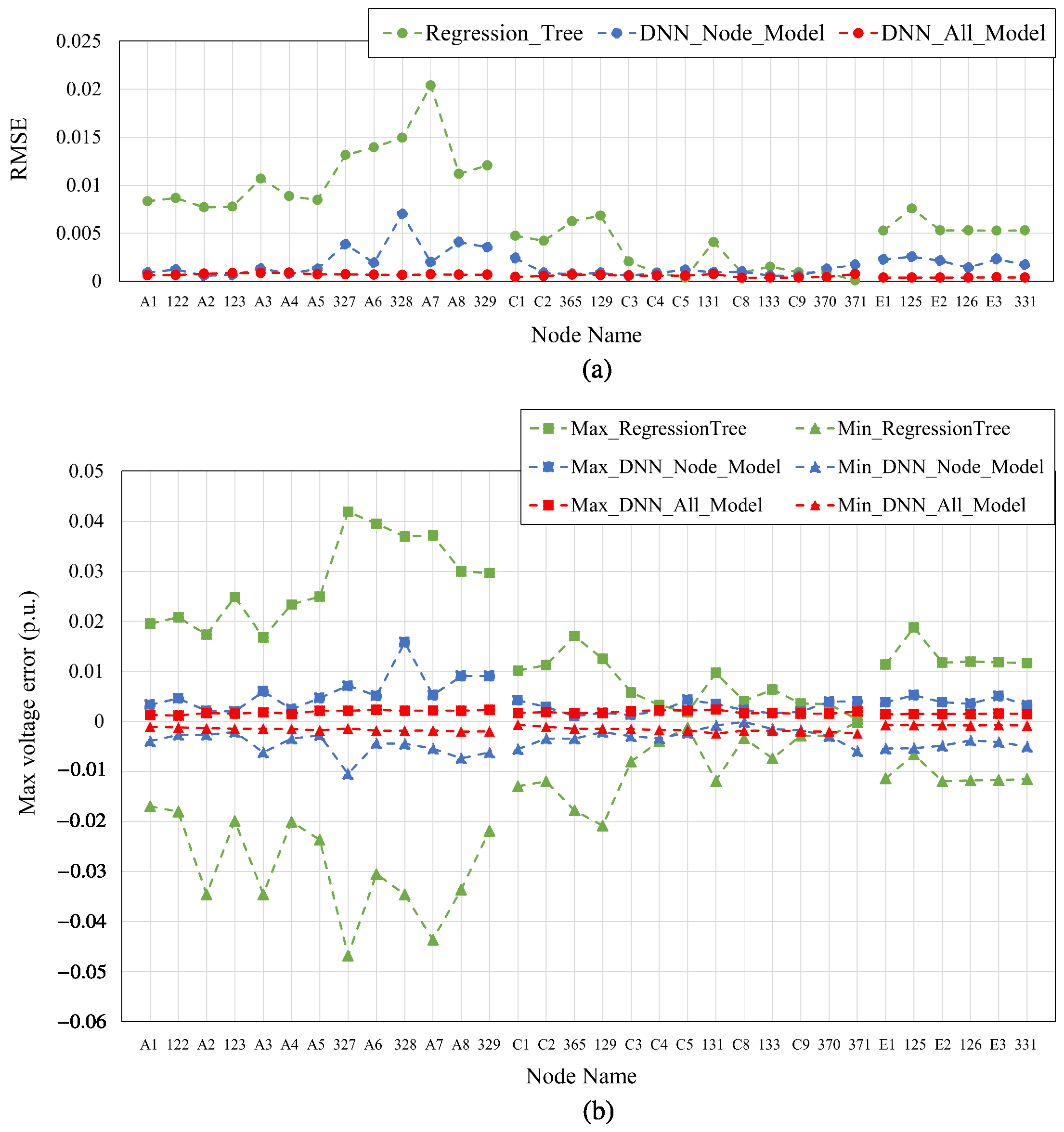
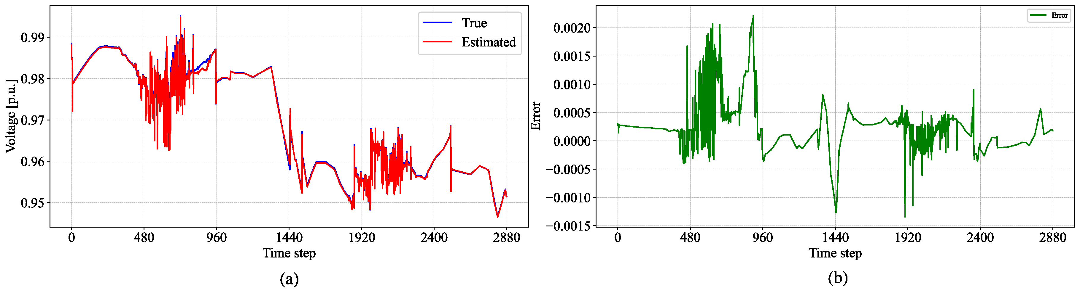
The proposed “ALL Model”, which consolidates all nodes into a single DNN model, achieved remarkable accuracy in voltage estimation. It showed notable improvements in reducing RMSE and maximum estimation errors across the test dataset. In particular, the maximum estimation error was 0.0024 p.u., indicating that this estimation accuracy does not affect the voltage control. The DNN ALL Model effectively captured nonlinear relationships, substantially outperforming the regression tree approach. The voltage estimation method demonstrated high accuracy, particularly in challenging places such as the end nodes of line A, where the estimation errors were notably reduced. In terms of voltage control, the proposed method successfully maintained proper voltage across all nodes while reducing the frequency of tap changes in response to fluctuating PV output. The integration of voltage estimation allowed for comprehensive grid monitoring and control, even in nodes traditionally difficult to regulate using benchmark methods. Notably, the voltage deviation observed in the benchmark model at node A8 was mitigated, highlighting the effectiveness of the proposed model’s policy. The proposed voltage control method had low communication costs because it uses only limited measurable information, and this method coordinates voltage regulators that are on different timescales in the grid to maintain proper voltage by implementing control based on estimated voltage.

Furthermore, the use of SHAP values offered valuable insights into the decision-making process of the DRL agent. By evaluating feature importance at both global and local levels, the analysis revealed key factors influencing control decisions, including tap position, PV active power output, and PCS reactive power output. The results demonstrated that the DNN-based model effectively utilized voltage information from other nodes, facilitating coordinated control across different lines. Additionally, the SHAP analysis provided an explanation for the effectiveness of the proposed method in maintaining proper voltage, in contrast to the benchmark model. The SHAP values offered a transparent mechanism for understanding the model’s decision-making process, providing important guidance for future improvements in the model.

In conclusion, the proposed DRL-based voltage control framework with DNN-based voltage estimation offered a significant advancement in grid voltage control by reducing deviations and enhancing accuracy. And, combined with SHAP-based interpretability, it provided a transparent mechanism for decision-making insights.

In the future, the proposed framework should be validated on larger and more complex grid models that more closely resemble real-world systems. This would allow for an assessment of the method’s scalability and robustness under more realistic conditions. Additionally, while this study utilized SHAP analysis to evaluate and explain the model’s performance, future research should focus on leveraging insights gained from SHAP values to further refine and improve the model. By incorporating these insights, it may be possible to enhance the model’s decision-making capabilities and achieve even better voltage control performance. These advancements will contribute to the continuous development of intelligent voltage control systems that are both practical and reliable for modern power grids.

References

1. Wang, Z. Key technologies in photovoltaic power generation systems. J. Phys. Conf. Ser. 2024, 2786, 012010. [Google Scholar] [CrossRef]
2. Gao, X.; Zhang, J.; Sun, H.; Liang, Y.; Wei, L.; Yan, C.; Xie, Y. A Review of Voltage Control Studies on Low Voltage Distribution Networks Containing High Penetration Distributed Photovoltaics. Energies 2024, 17, 3058. [Google Scholar] [CrossRef]
3. Mu, C.; Yan, M.; Quanlin, T.; Ling, Z.; Wenli, L.; Han, W. Optimization of Var-Voltage Regulation Control Strategy for Grid-Connected Inverter of Photovoltaic Power. IOP Conf. Ser. Earth Environ. Sci. 2021, 691, 012007. [Google Scholar] [CrossRef]
4. Chen, Q.; Bai, J.; Chen, X.; Wang, Y.; Wang, H.; Zhou, Y.; Wang, F.; Dong, N. Analysis of the impact of distributed photovoltaic grid integration on distribution network voltage. J. Phys. Conf. Ser. 2024, 2703, 012047. [Google Scholar] [CrossRef]
5. Iioka, D.; Fujii, T.; Orihara, D.; Tanaka, T.; Harimoto, T.; Shimada, A.; Goto, T.; Kubuki, M. Voltage reduction due to reverse power flow in distribution feeder with photovoltaic system. Int. J. Electr. Power Energy Syst. 2019, 113, 411–418. [Google Scholar] [CrossRef]
6. Jin, L.; Gong, X.; Sun, Q.; Sha, M. Reactive PowerControl of Grid-Connected Photovoltaic Power Generation. J. Phys. Conf. Ser. 2021, 1754, 012001. [Google Scholar] [CrossRef]
7. Alrumayh, O.; Sayed, K.; Almutairi, A. LVRT and Reactive Power/Voltage Support of Utility-Scale PV Power Plants during Disturbance Conditions. Energies 2023, 16, 3245. [Google Scholar] [CrossRef]
8. Iioka, D.; Fujii, T.; Tanaka, T.; Harimoto, T.; Motoyama, J. Voltage Reduction in Medium Voltage Distribution Systems Using Constant Power Factor Control of PV PCS. Energies 2020, 13, 5430. [Google Scholar] [CrossRef]
9. Singhal, A.; Ajjarapu, V.; Fuller, J.; Hansen, J. Real-Time Local Volt/Var Control Under External Disturbances with High PV Penetration. IEEE Trans. Smart Grid 2019, 10, 3849–3859. [Google Scholar] [CrossRef]
10. IEEE Std 1547-2018; Revision of IEEE Std 1547-2003; IEEE Standard for Interconnection and Interoperability of Distributed Energy Resources with Associated Electric Power Systems Interfaces. IEEE Standard: Piscataway, NJ, USA, 2018; pp. 1–138. [CrossRef]
11. Xu, Y.; Dong, Z.Y.; Zhang, R.; Hill, D.J. Multi-Timescale Coordinated Voltage/Var Control of High Renewable-Penetrated Distribution Systems. IEEE Trans. Power Syst. 2017, 32, 4398–4408. [Google Scholar] [CrossRef]
12. Savasci, A.; Inaolaji, A.; Paudyal, S. Two-Stage Volt-VAr Optimization of Distribution Grids With Smart Inverters and Legacy Devices. IEEE Trans. Ind. Appl. 2022, 58, 5711–5723. [Google Scholar] [CrossRef]
13. Xu, H.; Dominguez-Garcia, A.D.; Sauer, P.W. A Data-driven Voltage Control Framework for Power Distribution Systems. In Proceedings of the 2018 IEEE Power & Energy Society General Meeting (PESGM), Portland, OR, USA, 5–10 August 2018; IEEE: Piscataway, NJ, USA; pp. 1–5. [Google Scholar] [CrossRef]
14. Chen, X.; Qu, G.; Tang, Y.; Low, S.; Li, N. Reinforcement Learning for Selective Key Applications in Power Systems: Recent Advances and Future Challenges. IEEE Trans. Smart Grid 2022, 13, 2935–2958. [Google Scholar] [CrossRef]
15. Xu, H.; Dominguez-Garcia, A.D.; Sauer, P.W. Optimal Tap Setting of Voltage Regulation Transformers Using Batch Reinforcement Learning. IEEE Trans. Power Syst. 2020, 35, 1990–2001. [Google Scholar] [CrossRef]
16. Duan, J.; Shi, D.; Diao, R.; Li, H.; Wang, Z.; Zhang, B.; Bian, D.; Yi, Z. Deep-Reinforcement-Learning-Based Autonomous Voltage Control for Power Grid Operations. IEEE Trans. Power Syst. 2020, 35, 814–817. [Google Scholar] [CrossRef]
17. Wang, W.; Yu, N.; Gao, Y.; Shi, J. Safe Off-Policy Deep Reinforcement Learning Algorithm for Volt-VAR Control in Power Distribution Systems. IEEE Trans. Smart Grid 2020, 11, 3008–3018. [Google Scholar] [CrossRef]
18. Cao, D.; Hu, W.; Zhao, J.; Huang, Q.; Chen, Z.; Blaabjerg, F. A Multi-Agent Deep Reinforcement Learning Based Voltage Regulation Using Coordinated PV Inverters. IEEE Trans. Power Syst. 2020, 35, 4120–4123. [Google Scholar] [CrossRef]
19. Hai, D.; Zhu, T.; Duan, S.; Huang, W.; Li, W. Deep Reinforcement Learning for Volt/VAR Control in Distribution Systems: A Review. In Proceedings of the 2022 5th International Conference on Energy, Electrical and Power Engineering (CEEPE), Chongqing, China, 22–24 April 2022; pp. 596–601. [Google Scholar] [CrossRef]
20. Liu, H.; Wu, W.; Wang, Y. Bi-Level Off-Policy Reinforcement Learning for Two-Timescale Volt/VAR Control in Active Distribution Networks. IEEE Trans. Power Syst. 2023, 38, 385–395. [Google Scholar] [CrossRef]
21. Cao, D.; Zhao, J.; Hu, W.; Yu, N.; Ding, F.; Huang, Q.; Chen, Z. Deep Reinforcement Learning Enabled Physical-Model-Free Two-Timescale Voltage Control Method for Active Distribution Systems. IEEE Trans. Smart Grid 2022, 13, 149–165. [Google Scholar] [CrossRef]
22. Zhang, T.; Yu, L.; Yue, D.; Dou, C.; Xie, X.; Hancke, G.P. Two-Timescale Coordinated Voltage Regulation for High Renewable-Penetrated Active Distribution Networks Considering Hybrid Devices. IEEE Trans. Ind. Inform. 2024, 20, 3456–3467. [Google Scholar] [CrossRef]
23. Vijaychandra, J.; Prasad, B.R.V.; Darapureddi, V.K.; Rao, B.V.; Knypinski, t. A Review of Distribution System State Estimation Methods and Their Applications in Power Systems. Electronics 2023, 12, 603. [Google Scholar] [CrossRef]
24. Primadianto, A.; Lu, C.N. A Review on Distribution System State Estimation. IEEE Trans. Power Syst. 2017, 32, 3875–3883. [Google Scholar] [CrossRef]
25. Carcangiu, S.; Fanni, A.; Pegoraro, P.A.; Sias, G.; Sulis, S. Forecasting-Aided Monitoring for the Distribution System State Estimation. Complexity 2020, 2020, 1–15. [Google Scholar] [CrossRef]
26. Setta, T.; Aoki, M.; Ohori, R.; Verma, S.C.; Shimono, A. A Study on Voltage Estimation Methodology using Regression Tree for High Voltage System. IEEJ Trans. Power Energy 2020, 140, 495–503. [Google Scholar] [CrossRef]
27. Ito, R.; Matsushima, F.; Aoki, M.; Ueda, K.; Verma, S.C.; Nakatsui, S. A Voltage and Reactive Power Control Method Based on Sequential Updated Control Targets Considering Machine Learning Enabled Customer Voltage Estimation. In Proceedings of the 2023 International Conference on Sustainable Technology and Engineering (i-COSTE), Nadi, Fiji, 4–6 December 2023; pp. 1–5. [Google Scholar] [CrossRef]
28. Matsushima, F.; Aoki, M.; Ueda, K.; Verma, S.C.; Nakatsui, S. The Voltage and Reactive Power Control Methodology for Sub-transmission Network using Machine Learning. IEEJ Trans. Power Energy 2024, 144, 474–483. [Google Scholar] [CrossRef]
29. Wu, G.; Liu, S.; Xie, T.; Luo, W.; Liu, J. Fast power flow calculation method for power system based on heterogeneous edge graph convolutional neural network. J. Phys. Conf. Ser. 2024, 2781, 012014. [Google Scholar] [CrossRef]
30. Machlev, R.; Heistrene, L.; Perl, M.; Levy, K.; Belikov, J.; Mannor, S.; Levron, Y. Explainable Artificial Intelligence (XAI) techniques for energy and power systems: Review, challenges and opportunities. Energy AI 2022, 9, 100169. [Google Scholar] [CrossRef]
31. Kuzlu, M.; Cali, U.; Sharma, V.; Guler, O. Gaining Insight Into Solar Photovoltaic Power Generation Forecasting Utilizing Explainable Artificial Intelligence Tools. IEEE Access 2020, 8, 187814–187823. [Google Scholar] [CrossRef]
32. Zhang, K.; Zhang, J.; Xu, P.D.; Gao, T.; Gao, D.W. Explainable AI in Deep Reinforcement Learning Models for Power System Emergency Control. IEEE Trans. Comput. Soc. Syst. 2022, 9, 419–427. [Google Scholar] [CrossRef]
33. Matsushima, F.; Ryuto, K.; Aoki, M.; Yuta, N.; Verma, S.C.; Katsuhisa, U. Voltage estimation method using deep neural network considering PCS reactive power control in sub-transmission systems. In Proceedings of the Joint Technical Meeting on Power Engineering/Power Systems Engineering, online conference, 19–20 September 2024; Volume 2, pp. 99–104. [Google Scholar]
34. Matsushima, F.; Aoki, M.; Ueda, K.; Verma, S.C.; Nakatsui, S. Multi-Timescale Voltage and Reactive Power Control Method Combining Fast PV PCS and Slow Transformer Tap Response Using Deep Reinforcement Learning. In Proceedings of the 2023 International Conference on Sustainable Technology and Engineering (i-COSTE), Nadi, Fiji, 4–6 December 2023; Volume 754, pp. 1–6. [Google Scholar] [CrossRef]
35. Fujimoto, S.; van Hoof, H.; Meger, D. Addressing Function Approximation Error in Actor-Critic Methods. arXiv 2018. [Google Scholar] [CrossRef]
36. Bellemare, M.G.; Dabney, W.; Munos, R. A Distributional Perspective on Reinforcement Learning. arXiv 2017. [Google Scholar] [CrossRef]
37. Institute of Electrical Engineer of Japan (IEEJ) standard model. In Technical Report, Technical Report of the Institute of Electrical Engineers of Japan; Institute of Electrical Engineers of Japan: Tokyo, Japan, 1999; Volume 754.
38. Cao, D.; Zhao, J.; Hu, W.; Ding, F.; Huang, Q.; Chen, Z.; Blaabjerg, F. Data-Driven Multi-Agent Deep Reinforcement Learning for Distribution System Decentralized Voltage Control with High Penetration of PVs. IEEE Trans. Smart Grid 2021, 12, 4137–4150. [Google Scholar] [CrossRef]
Figure 1. Configuration of control and monitoring system for a sub-transmission grid.
Energies 18 00653 g001
Figure 2. Requirements for proper voltage in the sub-transmission grid.
Energies 18 00653 g002
Figure 3. Flowchart of the proposed method.
Energies 18 00653 g003
Figure 4. Overview diagram of multi-timescale voltage control.
Energies 18 00653 g004
Figure 5. Algorithm of training agents.
Energies 18 00653 g005
Figure 6. Algorithm of real-time execution.
Energies 18 00653 g006
Figure 7. Sub-transmission grid model with large-scale PVs.
Energies 18 00653 g007
Figure 8. Test data for DRL training. (a) Load profile of each customer. (b) PV output profile.
Energies 18 00653 g008
Figure 9. Maximum estimation error and RMSE of conventional regression tree and proposed DNN method. (a) RMSE. (b) Maximum estimation error in the positive (Max) and negative (Min) directions.
Energies 18 00653 g009
Figure 10. (a) Total reward profile of training process. (b) Maximum voltage differences from center voltage profile of training process.
Energies 18 00653 g010
Figure 11. Control results of the proposed voltage control with voltage estimation. (a) Difference from the center voltage. (b) Tap position of LRT. (c) Reactive power output of PCSs.
Energies 18 00653 g011
Figure 12. Voltage estimation error in test data at node A8. (a) True and estimated voltage at node A8. (b) Difference between true and estimated voltage at node A8.
Energies 18 00653 g012
Figure 13. Control results of the benchmark voltage control. (a) Difference from the center voltage. (b) Tap position of LRT. (c) Reactive power output of PCSs.
Energies 18 00653 g013
Figure 14. SHAP summary plot for the proposed PCS agent. (a) SHAP analysis for PCS at node C6 of the actor network. (b) SHAP analysis for PCS at node C7 of the actor network. (c) SHAP analysis for PCS at node C10 of the actor network. (d) SHAP analysis for the critic network.
Energies 18 00653 g014
Figure 15. SHAP summary plot for the proposed LRT agent. (a) SHAP analysis for the no-tap-change action. (b) SHAP analysis for the tap-down action. (c) SHAP analysis for the tap-up action.
Energies 18 00653 g015
Figure 16. SHAP waterfall plots for the proposed PCS agent. (a) SHAP analysis for PCS at node C6 within the actor network. (b) SHAP analysis for PCS at node C7 within the actor network. (c) SHAP analysis for PCS at node C10 within the actor network.
Energies 18 00653 g016
Figure 17. SHAP waterfall plots for the proposed LRT agent. (a) SHAP analysis for the no-tap-change action. (b) SHAP analysis for the tap-down action. (c) SHAP analysis for the tap-up action.
Energies 18 00653 g017