Optimal Configuration Strategy of Soft Open Point in Flexible Distribution Network Considering Reactive Power Sources

Abstract

The intelligent soft open point (SOP) has powerful power flow regulation capabilities in the distribution network. If applied to the distribution network, it can flexibly cope with the output uncertainty of unmanageable distributed energy sources. However, considering the investment, operation, and maintenance costs, as well as the assistance of reactive power equipment, the site selection and capacity determination of SOP have become an urgent problem to be solved. This article proposes the optimal configuration strategy of SOP in a flexible interconnected distribution network, taking into account the features of distributed generation and reactive power sources. Firstly, based on the unpredictability of DG output, this paper uses improved sensitivity analysis to determine the optimal SOP installation location. Subsequently, with the optimization objective of minimizing the annual cost of the distribution network, this paper considers the characteristics of DGs, CBs, and OLCTs and uses second-order cone programming to optimize and solve SOP capacity under constraints such as trends. Finally, in the enhanced IEEE 33-node distribution system model, the effects of different scenarios on node voltage, reactive power components, and SOP location and capacity are compared.

1. Introduction

With the continuous improvement of the penetration rate of distributed new energy in the power distribution grid, the power distribution grid is developing rapidly towards high power electronification. Although DG integration is beneficial for minimizing system power loss, enhancing power supply reliability, and decreasing environmental pollution, the output of renewable distributed power sources such as photovoltaics and wind turbines is greatly affected by temperature, wind speed, and air pressure, and has obvious randomness and volatility in [1]. This leads to increasingly complex power flow distribution during the operation of the distribution network, which can easily trigger problems such as voltage exceeding limits, network congestion, and bidirectional power flow in [2,3,4,5]. In response to the complexity brought by the large-scale integration of renewable energy into system operation, how to plan and construct a more flexible basic distribution system to allocate system resources in real time and quickly achieve supply–demand balance has attracted widespread attention from academia and industry.

In current distribution networks, Voltage and Var Control (VVC) is primarily achieved through the regulation of primary equipment such as on-load tap changers (OLTCs), switchable capacitor banks (CBs), tie switches, and the direct management of dispatchable distributed generators (DGs) as described in [6]. However, the traditional methods of OLTC tap adjustment, CB switching, and tie switch reconfiguration face limitations due to their slow response times and discrete voltage control capabilities. As a result, it becomes challenging to achieve real-time, high-precision VVC, especially when distributed generators and loads experience frequent fluctuations, as noted in [7]. To address the issues of declining inertia and reduced frequency modulation capabilities in power systems with a high proportion of new energy, many countries, including China, Denmark, and the United Kingdom, have proposed friendly grid connection requirements for new energy plants to possess certain frequency modulation capabilities. The doubly fed induction generator (DFIG), representing variable-speed wind turbines, has a broad range of operating speeds, providing an energy source for frequency modulation power. Additionally, the flexible and rapid response characteristics of converters enable DFIGs to respond quickly to frequency fluctuations in the system, simulating the inertial response of synchronous machines. Therefore, utilizing the potential frequency modulation capacity of wind farms to improve the frequency response characteristics of the new power system has become a research hotspot in recent years. The intelligent soft switch SOP has strong power flow regulation capabilities in the power distribution grid. If applied to the power distribution grid, it can flexibly cope with the uncertainty of uncontrollable distributed power output, thereby improving the operation status and efficiency of the power distribution grid, and increasing the consumption rate of renewable energy. However, the implementation of SOP’s real-time and precise power control function mainly relies on expensive fully controlled power electronic devices. Therefore, in the planning stage, it is necessary to fully consider its investment costs in order to achieve a reasonable allocation of SOP.

Reference [8] briefly describes the basic principles and models of SOP, and it highlights that SOP can significantly enhance the integration capacity of distributed power generation. The authors in [9,10] conducted simulation analysis on the steady-state and transient operating characteristics of SOP, but the SOP planning problem has not yet been addressed. In addition, reference [11] proposed an SOP optimization configuration method that considers the coordination of network capacity expansion and reactive power support. By establishing an SOP power model that takes into account the connection line and SOP power flow direction, and considering the influence of SOP connection switch status on power flow and network topology, the SOP capacity is optimized. However, the above references did not consider the impact of system power changes resulting from the randomness and instability of distributed generation (DG) on system voltage, as well as the capability of SOP to regulate and stabilize the system voltage. Reference [12] puts forward a mixed integer nonlinear optimization problem, which optimally determines the location and size of SOP based on typical operation scenarios generated by Wasserstein distance. This paper discusses the influence of DG operation characteristics on SOP planning. Reference [13] not only considers DG uncertainty, but also plans DG while planning and configuring SOP, but the above references do not consider the influence of sensitivity calculation on SOP planning and capacity allocation. Reference [14] proposed an intelligent soft switch SOP optimization configuration method based on opportunity-constrained programming, considering the strong coupling between SOP operation strategy and random output of distributed power sources. The optimal goal was to reduce the total annual cost, and an SOP site selection and capacity model was established based on opportunity constraints. The calculation provided a new method for SOP optimization configuration, but ignored the influence of reactive components on SOP capacity, resulting in overly conservative optimization results.

In summary, the reactive power sources, OLTCs and CBs, in the distribution network compensate for reactive power near the installation nodes, thereby reducing voltage drop and line losses, and affecting the installation location and capacity of SOP. In response to the above issues, this article proposes the optimal configuration strategy of SOP in a flexible interconnected distribution network considering the characteristics of distributed generation and reactive power sources. Firstly, based on the uncertainty of DG output, this paper uses improved sensitivity analysis to determine the optimal SOP installation location. Subsequently, with the optimization objective of minimizing the annual cost of the distribution network, this paper considers the characteristics of DGs, CBs, and OLCTs and uses mixed-integer second-order cone programming to optimize and solve SOP capacity under constraints such as trends. Finally, in the enhanced IEEE 33-node distribution system model, the effects of different scenarios on node voltage, reactive power components, and SOP location and capacity are compared.

2. Function and Model of Soft Open Point

2.1. Improved Sensitivity Analysis

SOP is a sophisticated distribution management technology primarily deployed at conventional contact switch locations. Figure 1 illustrates the topology of two AC/DC hybrid distribution zones, where the SOP installation points are highlighted within the dashed box, facilitating flexible interconnection between feeder terminals or substations. The system utilizes the power output of two converters as control variables, considering the losses in the converters while maintaining operational efficiency. Thanks to the isolating effect of the DC system, the reactive power outputs of the two converters are independent, with each converter only required to operate within its own capacity limits. It is usually installed at the end of the feeder instead of the conventional contact switch.

During normal operation, the SOP controller provides instantaneous power regulation or continuous power regulation between interconnected feeders and supports two operating modes on two terminals, namely U_{dc_Q} mode and P_{_Q} mode. The former stabilizes the DC bus voltage and regulates reactive power through an inverter, while the latter regulates active and reactive power through an inverter, this enables it to dynamically regulate both active and reactive power according to varying conditions, making it the easiest and most rapidly developing form of flexible interconnection at present. In the event of a fault, SOP can isolate symmetrical and asymmetrical faults between interconnected feeders, thereby limiting the propagation of faults and the increase in short-circuit currents throughout the entire distribution system. The SOP working mode can seamlessly switch according to the actual distribution network, and the switching time can be in minutes or hours. This article uses a two-port inverter with an hourly scheduling time scale.

2.2. Model of Soft Open Point

This article takes the back-to-back voltage source converter as an example, and the SOP controllable variables include four, namely the active power and reactive power output by the two converters. Assuming that SOP injects power into the grid in the positive direction, the reactive power output by the two converters does not affect each other due to the isolation of the DC link and only needs to meet the capacity constraints of their respective converters. Building an SOP model involves the following constraints:

(1)

SOP active constraint

$$P_{S,i,t}+P_{S,j,t}+P_{S,i,t}^{loss}+P_{S,j,t}^{loss}=0$$

(1)

$$\left\{\begin{array}{l}{P}_{S,i,t}^{loss}=A_{S,i}\sqrt{{\left(P_{S,i,t}\right)}^2+{\left(Q_{S,i,t}\right)}^2}\hfill \\ P_{S,j,t}^{loss}=A_{S,j}\sqrt{{\left(P_{S,i,t}\right)}^2+{\left(Q_{S,i,t}\right)}^2}\hfill \end{array}\right.$$

(2)

(2)

SOP reactive power constraint

$$\left\{\begin{array}{l}{\underset{¯}{Q}}_{SOP,i,t}⩽Q_{SOP,i,t}⩽{\overline{Q}}_{SOP,i,t}\hfill \\ {\underset{\_}{Q}}_{SOP,j,t}⩽Q_{SOP,j,t}⩽{\overline{Q}}_{SOP,j,t}\hfill \end{array}\right.$$

(3)

(3)

SOP capacity constraint

$$\left\{\begin{array}{l}\sqrt{P_{SOP,i,t}^2+Q_{SOP,i,t}^2}⩽S_{SOP,i,t}\hfill \\ \sqrt{P_{SOP,j,t}^2+Q_{SOP,j,t}^2}⩽S_{SOP,j,t}\hfill \end{array}\right.$$

(4)

where P_SOP,i,t and P_SOP,j,t are the injecting power at node i and node j; S_SOP,j,t and S_SOP,j,t are the active losses of SOP at node i and node j; Q_SOP,i,t, and Q_SOP,j,t are the reactive power at node i and node j.

3. Optimal Configuration of Soft Open Point

Solving the SOP site selection problem involves dealing with a complex nonlinear combination problem with multiple dimensions. To simplify the complexity of the problem, this paper proposes a phased strategy for solving SOP site selection and capacity. In reaction to the issue of SOP access, this article uses an enhanced sensitivity analysis technique for identifying the optimal access location of SOP in [15]. To address the capacity issue of SOP, use the SOCP algorithm to optimize and settle the capacity of SOP.

3.1. Main Function of Soft Open Point

By performing a first-order Taylor expansion of the power balance equation at the system nodes, the relationship between the voltage change ΔV and the variations in active power ΔP and reactive power ΔQ can be derived. This is accomplished by setting either the change in reactive power (ΔQ) or the change in active power (ΔP) to zero.

$$\left\{\begin{array}{l}\Delta U^{\mathrm{T}}=\lambda \Delta P^{\mathrm{T}}\hfill \\ \Delta U^{\mathrm{T}}=\gamma \Delta Q^{\mathrm{T}}\hfill \end{array}\right.$$

(5)

where ΔU^T is the voltage variation matrix of node i; λ and γ are sensitivity matrices corresponding to P and Q.

Further expanding on λ and γ, the following analytical formula can be obtained:

$$\lambda =\left[\begin{array}{ccccc}{\lambda }_{11}& \cdots & {\lambda }_{1i}& \cdots & {\lambda }_{1(n-1)}\\ ⋮& & ⋮& & ⋮\\ {\lambda }_{j1}& \cdots & {\lambda }_{ji}& \cdots & {\lambda }_{j(n-1)}\\ ⋮& & ⋮& & ⋮\\ {\lambda }_{(n-1)1}& \cdots & {\lambda }_{(n-1)i}& \cdots & {\lambda }_{(n-1)(n-1)}\end{array}\right]$$

(6)

$$\gamma =\left[\begin{array}{ccccc}{\gamma }_{11}& \cdots & {\gamma }_{1i}& \cdots & {\gamma }_{1(n-1)}\\ ⋮& & ⋮& & ⋮\\ {\gamma }_{j1}& \cdots & {\gamma }_{ji}& \cdots & {\gamma }_{j(n-1)}\\ ⋮& & ⋮& & ⋮\\ {\gamma }_{(n-1)1}& \cdots & {\gamma }_{(n-1)i}& \cdots & {\gamma }_{(n-1)(n-1)}\end{array}\right]$$

(7)

where n is the number of nodes; λ_ji and γ_ji are the responsiveness of the active and reactive power changes at node i to the voltage at node j. The matrices composed of λ_ji and γ_ji are the matrices representing the sensitivity of active and reactive power.

With the integration of DG, the voltage distribution pattern in the power distribution grid has shifted. Representing the node voltage sensitivity using Equation (5) becomes challenging, increasing the risk of voltage exceeding acceptable limits. Considering the operating characteristics of the entire new distribution station area over a 24 h period, this paper proposes a modification to the traditional sensitivity calculation method by introducing node voltage deviation, expressed as

$$\left\{\begin{array}{l}{S}_{ji}=\left({\mathsf{\omega }}_{\mathrm{l}}{\lambda }_{ji.t}+\left(1-{\mathsf{\omega }}_{\mathrm{l}}\right){\gamma }_{ji,t}\right){\mu }_{j,t}\hfill \\ {\mu }_{j,t}=\mathrm{var}(U_{j,t})\hfill \end{array}\right.$$

(8)

where, in the formula, S_ji is the redefined node sensitivity value; µ_j,t is the difference between the actual voltage and the expected voltage; var (U_j,t) is the magnitude of voltage fluctuation at node j, and the variance of the 24 h voltage at that node is taken; ω₁ is the weight coefficient of voltage active and reactive sensitivity (0 < ω₁ < 1), which is determined by considering the system power variation in [15], where ω₁ = 0.6.

Due to the instability and intermittency of DG, its output will change in sequence, so the optimization configuration of SOP in active distribution networks needs to consider the issue of DG timing changes and further improve the sensitivity calculation, expressed as follows:

$$\left\{\begin{array}{ll}{S}_{ji}={\displaystyle \sum _{t=1}^{24}{S}_{ji,t}{\epsilon }_t}\hfill & \\ {\epsilon }_t=(n_t+1)\max \hfill & \left|U_{k,\mathrm{t}}-U_{0,k,\mathrm{t}}\right|\\ & \mathrm{k}=1,2,\cdot \cdot \cdot ,n-1\end{array}\right.$$

(9)

where S_ji represents the sensitivity of the power change at node i with respect to the voltage at node j; ɛ_t is the weight of time period t; n_t is the number of nodes in the system with voltage exceeding the limit during time period t; Max |U_k,t−U_0,k,t| is the maximum node voltage offset value during time period t.

The larger the sensitivity value S_ji after improvement, the greater the impact of power changes on voltage, indicating that it is more necessary to connect the node to SOP.

3.2. Optimal Model of Soft Open Point

Taking into full consideration the impact of OLTC and CBs on SOP capacity configuration, this section aims to achieve the total system configuration cost, with system power flow constraints, SOP, OLTC, and CB operation constraints as the constraints, to solve for the configuration results under the optimal solution.

3.2.1. Objective Function

In this study, to address the allocation of SOP capacity, the objective function is defined by considering several factors: the annual investment costs, operation and maintenance costs, power loss costs, and switching losses. These elements are incorporated as part of the optimization process, as outlined in the following:

$$\min F=C_t+C_{\mathrm{w}}+C_{\mathrm{s}}+C_{switch}$$

(10)

(1)

The annual investment cost is obtained by amortizing the total investment cost over the service life of the system.

$$C_t={\displaystyle \frac{d{(1+d)}^y}{{(1+d)}^y-1}}{\displaystyle \sum _{k=1}^N{c}_k}{S}_k$$

(11)

where d is the discount rate; it is fixed at 0.05. y is the service life; it is fixed at 20. C_k and S_k are the cost of investment per unit of capacity and the capacity of the k-th SOP.

(2)

Maintenance cost per year:

$$C_{\mathrm{w}}=\eta {\displaystyle \sum _{k=1}^N{c}_k}{S}_k$$

(12)

where η is the maintenance factor; it is set to 0.02.

(3)

Loss cost of Soft Open Point

$$C_{\mathrm{s}}=365\mu {\displaystyle \sum _{i=1}^{n_t}{\displaystyle \sum _{t=1}^n(P_{i,t}+P_{S,i,t}^{\mathrm{loss}})}}\Delta T$$

(13)

where η is the Average electricity price, n is the number of nodes of SOP; ΔT is the duration. P_i,t is the sum of active power injected into this node.

(4)

Switching Loss

The total costs of switching operations include the adjustment cost of the OLTC and the switching cost of the CBs.

$$C_{switch}={\displaystyle \sum _{i,j\in \mathsf{\Omega }o}^{}{\displaystyle \sum _{t=1}^{N_t}(C_{tap}\left|K_{i,j,t}-K_{i,j,t-1}\right|)}}+{\displaystyle \sum _{i=1}^{N_{\mathrm{n}}}{\displaystyle \sum _{t=1}^{N_t}(C_{cap}\left|N_{i,t}^{CB}-N_{i-1,t}^{CB}\right|)}}$$

(14)

where N_t is the total periods of the time horizon, N_n total number of the nodes, C_tap, C_cap is the cost coefficients of OLTC and CBs, respectively, Ω_o is the set of branches with OLTC, K_i,j,t is a number of the tap steps of the OLTC connected to branch ij at period t, and $N_{i,t}^{CB}$ is a number of the CB units in operation at the node.

3.2.2. Constraints

The constraints consist of SOP operation constraints, power flow balance, second-order cone constraints, and current and voltage limitations, with Ohm’s law also considered. The following subsections provide detailed models for each of these constraints.

(1)

Power system operation constraints

This article uses DisFlow power flow constraints applicable to radial networks in [16]. Power system operation constraints include power balance constraints, system Ohm’s law constraints, voltage and current constraints, etc. The expressions are as follows;

$${\displaystyle \sum _{ij\in \mathsf{\psi }}(P_{i,j,t}-r_{i,j}{I}_{i,j,t}^2)+P_{i,t}+}{\displaystyle \sum _{j\in \mathsf{\Omega }o}{P}_{i,j,t}^{\mathrm{OLTC}}}={\displaystyle \sum _{ik\in \mathsf{\psi }}{P}_{i,k,t}+{\displaystyle \sum _{ik\in \mathsf{\Omega }o}{P}_{i,k,t}^{\mathrm{OLTC}}}}, 0⩽I_{i,j,t}^2⩽I_{\max }^2$$

(15)

$${\displaystyle \sum _{ij\in \mathsf{\psi }}(Q_{i,j,t}-x_{i,j}{I}_{i,j,t}^2)+Q_{i,t}+}{\displaystyle \sum _{j\in \mathsf{\Omega }o}{Q}_{i,j,t}^{\mathrm{OLTC}}}={\displaystyle \sum _{ik\in \mathsf{\psi }}{Q}_{i,k,t}+{\displaystyle \sum _{ik\in \mathsf{\Omega }o}{Q}_{i,k,t}^{\mathrm{OLTC}}}}$$

(16)

$$U_{i,t}^2-U_{j,t}^2-2\left(r_{i,j}{P}_{i,j,t}+x_{i,j}{Q}_{i,j,t}\right)+\left(r_{i,j}^2+x_{i,j}^2\right)I_{i,j,t}^2=0, U_{\min }^2⩽U_{i,t}^2⩽U_{\max }^2$$

(17)

$$I_{i,j,t}^2{U}_{i,j,t}^2=P_{i,j,t}^2+Q_{i,j,t}^2$$

(18)

$$P_{i,t}=P_{i,t}^{\mathrm{DG}}+P_{i,t}^{\mathrm{SOP}}-P_{i,t}^{\mathrm{Load}}$$

(19)

$$Q_{i,t}=Q_{i,t}^{\mathrm{DG}}+Q_{i,t}^{\mathrm{SOP}}+Q_{i,t}^{\mathrm{CB}}-Q_{i,t}^{\mathrm{Load}}$$

(20)

where Formulas (16) and (17), respectively, represent the active power and reactive power balance of node i at time t; the Ohm law of branch ij at period t can be expressed as Formula (18); Formula (19) is used to represent the current of each line; and constraints (20) and (21), respectively, represent node i. Q_i,t and P_i,t are injected reactive power and active power of node I; V_i and θ_ij are the voltage and phase angle difference; $P_{i,t}^{DG}$ and $Q_{i,t}^{DG}$ are the active and reactive power outputs by DG; U_min and U_max are the upper and lower voltage limits of node i; I_max is the upper current magnitude limit of the branch.

(2)

Operation constraints of uncontrollable distributed power supply

DG operation constraints include active power and reactive power constraints, and DG capacity constraints, expressed as follows;

$$P_{\mathrm{DG},i,t}^{}=P_{\mathrm{DG},i,t}^{ref}$$

(21)

$$Q_{\mathrm{DG},i,t}^{}=P_{\mathrm{DG},i,t}^{ref}\tan {\theta }_{DG,i}^{}$$

(22)

$$\sqrt{P_{\mathrm{DG},i,t}^2+Q_{\mathrm{DG},i,t}^2}<S_{\mathrm{DG},i}^{}$$

(23)

where $P_{DG,i,t}^{ref}$ is the forecasted value of DG.

(3)

OLTC Operation Constraints

OLTC operation constraints [17] include voltage constraints, operation step size constraints, tap change rate constraints, and tap change range constraints, expressed as follows;

$$U_{i,t}=k_{i,j,t}{U}_{j,t}$$

(24)

$$k_{i,j,t}=k_{i,j,0}+K_{i,j,t}\Delta k_{i,j}$$

(25)

$${\displaystyle \sum _{t=1}^{N_t}\left|K_{i,j,t}-K_{i,j,t-1}\right|}\le {\overline{\Delta }}_{\mathrm{OLTC}}$$

(26)

$$K_{\min }\le K_{i,j,t}\le K_{\max }$$

(27)

where U_i,t is voltage magnitude at node i at period t; k_i,j,t is the number of the turn ratio of the OLTC connected to branch ij at period t; k_i,j,0 and Δk_i,j is initial turn ratio and increment per step of OLTC connected to branch ij; ${\overline{\Delta }}_{\mathrm{OLTC}}$ is the maximum variation in tap steps of the OLTC in the considered time horizon; K_min and K_max are the upper and lower steps of OLTC connected to the branch.

(4)

CB Operation Constraints

CB constraints include injection reactive power constraints, unit change rate constraints, and unit operation quantity constraints, expressed as follows;

$$Q_{CB,i,t}=N_{CB,i,j,t}{q}_{CB,i}$$

(28)

$${\displaystyle \sum _{t=1}^{N_t}\left|N_{CB,i,t}-N_{CB,i,t-1}\right|}\le {\overline{\Delta }}_{\mathrm{CB}}$$

(29)

$$0\le N_{i,t}^{CB}\le N_{\max }$$

(30)

where Q_CB,i,t is reactive power injection by CBs at node i at period t; q_CB,i is the reactive power capacity of each unit of the CBs at node i; $N_{i,t}^{CB}$ is a number of the CB units in operation at node i at period t; ${\overline{\Delta }}_{\mathrm{CB}}$ is the maximum variation in the CB; N_max is the total number of CBs at node i.

3.2.3. Conversion to an SOCP Model

Due to the involvement of a large number of SOP continuous power output, OLTC tap conversion, and CBs unit switching in the above model, and the rapid increase in model dimensionality as calculations progress, this paper linearizes the original model through second-order cone programming and converts it into SOCP model in [18].

According to reference [19], constraints (2), (4), (16)–(18), and (24) include the squares of current, voltage and power. Linearization is realized by variable substitution, and the formula is as follows;

$$\left\{\begin{array}{l}2{\displaystyle \frac{P_{S,i,t}^{loss}}{\sqrt{2}{A}_{S,i}}}{\displaystyle \frac{P_{S,i,t}^{loss}}{\sqrt{2}{A}_{S,i}}}\ge {\left(P_{S,i,t}\right)}^2+{\left(Q_{S,i,t}\right)}^2\hfill \\ 2{\displaystyle \frac{P_{S,j,t}^{loss}}{\sqrt{2}{A}_{S,j}}}{\displaystyle \frac{P_{S,j,t}^{loss}}{\sqrt{2}{A}_{S,j}}}\ge {\left(P_{S,j,t}\right)}^2+{\left(Q_{S,j,t}\right)}^2\hfill \end{array}\right.$$

(31)

$$\left\{\begin{array}{l}{P}_{SOP,i,t}^2+Q_{SOP,i,t}^2⩽{\displaystyle \frac{S_{SOP,i,t}}{\sqrt{2}}}{\displaystyle \frac{S_{SOP,i,t}}{\sqrt{2}}}2\hfill \\ P_{SOP,j,t}^2+Q_{SOP,j,t}^2⩽{\displaystyle \frac{S_{SOP,j,t}}{\sqrt{2}}}{\displaystyle \frac{S_{SOP,j,t}}{\sqrt{2}}}2\hfill \end{array}\right.$$

(32)

$${\displaystyle \sum _{ij\in \mathsf{\psi }}(P_{i,j,t}-r_{i,j}{\xi }_{i,j,t}^{})+P_{i,t}+}{\displaystyle \sum _{j\in \mathsf{\Omega }o}{P}_{i,j,t}^{\mathrm{OLTC}}}={\displaystyle \sum _{ik\in \mathsf{\psi }}{P}_{i,k,t}+{\displaystyle \sum _{ik\in \mathsf{\Omega }o}{P}_{i,k,t}^{\mathrm{OLTC}}}}$$

(33)

$${\displaystyle \sum _{ij\in \mathsf{\psi }}(Q_{i,j,t}-x_{i,j}{\xi }_{i,j,t}^{})+Q_{i,t}+}{\displaystyle \sum _{j\in \mathsf{\Omega }o}{Q}_{i,j,t}^{\mathrm{OLTC}}}={\displaystyle \sum _{ik\in \mathsf{\psi }}{Q}_{i,k,t}+{\displaystyle \sum _{ik\in \mathsf{\Omega }o}{Q}_{i,k,t}^{\mathrm{OLTC}}}}$$

(34)

$${\mu }_{i,t}^2-{\mu }_{j,t}^2-2\left(r_{i,j}{P}_{i,j,t}+x_{i,j}{Q}_{i,j,t}\right)+\left(r_{i,j}^2+x_{i,j}^2\right){\xi }_{i,j,t}^2=0$$

(35)

$$U_{\min }^2⩽{\mu }_{i,j,t}^{}⩽U_{\max }^2$$

(36)

$$0⩽{\xi }_{i,j,t}^{}⩽I_{\max }^2$$

(37)

where µ_i,t, ξ_i,_j,t are intermediate variables, µ_i,j,t = $U_{i.j.t}^2$ and ξ_i,j,t = $I_{i.j.t}^2$.

After variable substitution, Formula (19) remains a nonlinear constraint, and the relaxed second-order cone constraint is as follows;

$${‖{\left[2P_{i,j,t}2Q_{i,j,t}{\xi }_{i,j,t}-{\mu }_{i,t}\right]}^{\mathrm{T}}‖}_2\le {\xi }_{i,j,t}+{\mu }_{i,j,t}$$

(38)

The constraint (25) and its additional constraints after variable replacement are as follows;

$${\mu }_{i,t}={\displaystyle \sum _{k=0}^{2K_{\max }}\left[{\left(k_{i,j,0}+\left(k-K_{\max }\right)\Delta k_{i,j}\right)}^2{\mathsf{\varphi }}_{k,i,j,t}\right]}$$

(39)

$$U_{\min }^2{n}_{k,i,j,t}\le {\mathsf{\varphi }}_{k,i,j,t}\le U_{\max }^2{n}_{k,i,j,t} , n_{k,i,j,t}\in \left\{0,1\right\}$$

(40)

$$U_{\min }^2\left(1-n_{k,i,j,t}\right)\le {\mu }_{j,t}-{\mathsf{\varphi }}_{k,i,j,t}\le U_{\max }^2\left(1-n_{k,i,j,t}\right) , n_{k,i,j,t}\in \left\{0,1\right\}$$

(41)

where ф is the intermediate variable, ф = µ_i,j,t·n_k,i,j,t.

For the objective functions (15) and related constraints (27) and (30) of OLTC and CB, auxiliary variables $K_{i,j,t}^{+}$, $K_{i,j,t}^{-}$, $N_{i,j,t}^{+}$, $N_{i,j}^{+}$, t are introduced for linearization. The expression is as follows:

$${\displaystyle \sum _{t=1}^{N_t}\left({\mathrm{X}}_{i,j,t}-X_{i,j,t-1}\right)}\le {\overline{\Delta }}_{\mathrm{Y}}\mathrm{X}\in \left\{K,N\right\}\mathrm{Y}\in \left\{OLTC,CB\right\}$$

(42)

$${\mathrm{X}}_{i,j,t}-X_{i,j,t-1}={\mathrm{X}}_{i,j,t}^{+}-{\mathrm{X}}_{i,j,t}^{-}$$

(43)

$${\mathrm{X}}_{i,j,t}^{+}\ge 0,{ \mathrm{X}}_{i,j,t}^{-}\ge 0$$

(44)

$$C_{switch}={\displaystyle \sum _{i,j\in \mathsf{\Omega }o}^{}{\displaystyle \sum _{t=1}^{N_t}(C_{tap}\left(K_{i,j,t}^{+}-K_{i,j,t}^{-}\right))}}+{\displaystyle \sum _{i=1}^{N_{\mathrm{n}}}{\displaystyle \sum _{t=1}^{N_t}(C_{cap}\left(N_{i,t}^{+}-N_{i-1,t}^{-}\right))}}$$

(45)

At this point, after variable replacement and second-order cone relaxation, the original model is transformed into the SOCp model.

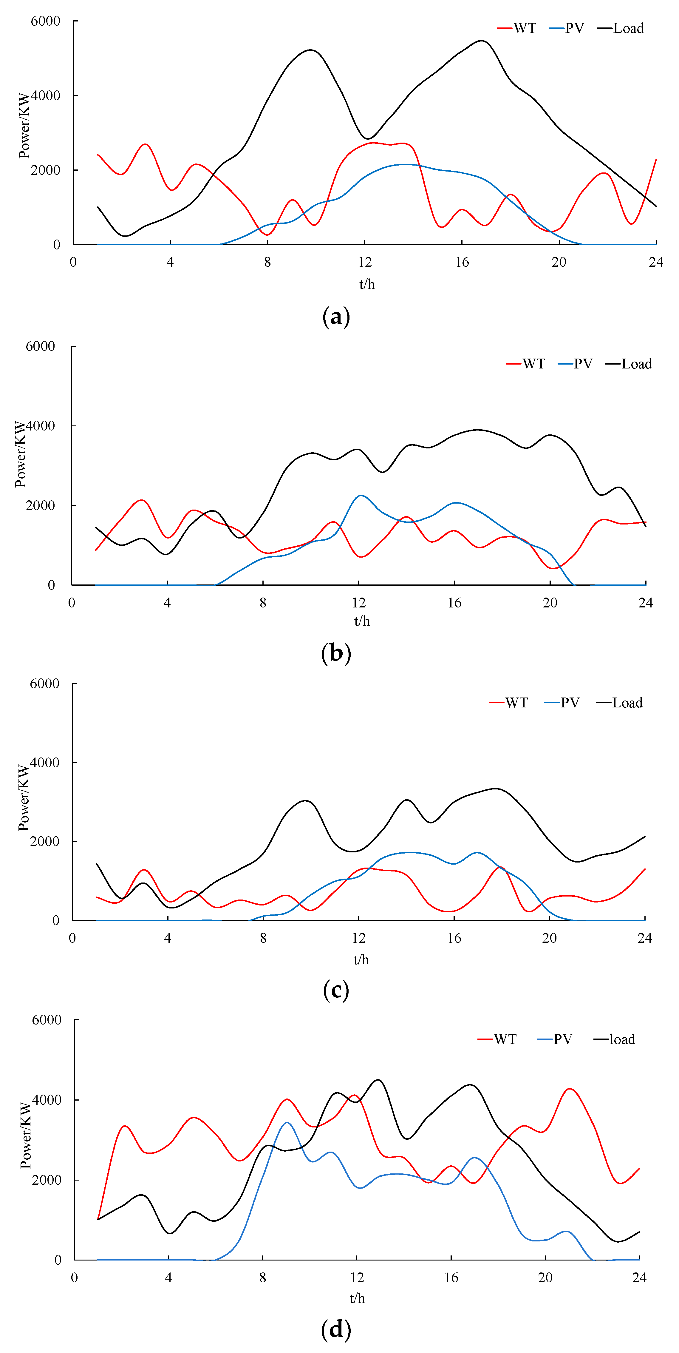
4. Simulation Results

This study uses an enhanced IEEE33 node distribution system to evaluate the effectiveness of the proposed method for optimizing SOP site selection and capacity. The system’s input and structure are illustrated in Figure 2 and Figure 3, while the node load and branch impedance details can be found in reference [17]. To account for the impact of high DG penetration on voltage limit violations, 3 PV units and 5 wind turbines (WTs) are integrated into the system. The PV units are installed at nodes 7, 13, and 27, while the WTs are placed at nodes 10, 16, 17, 30, and 33. The PVs operate at unity power factor, alongside the WTG. Load forecasting provides the hourly system load profile, and DG outputs are processed similarly. The optimization is implemented using the YALMIP toolbox on the MATLAB R2020a platform, with the IBMILOG CPLEX12.6 solver applied for SOP site selection and capacity optimization. The system node voltage is constrained to stay within 95% to 105% of the rated voltage.

The improved sensitivity analysis method proposed in this article was used to analyze and calculate 24 h a day. The calculation results are shown in Figure 4. This article sets the number of SOP interventions as 1, the SOP service life as 20 ¥, the SOP unit capacity investment cost as 1000 yuan/kVA, and the SOP converter loss coefficient, SOP annual operation and maintenance cost coefficient, and distribution system annual power loss cost coefficient is set to 0.02, 0.01, and 0.08, respectively.

To better validate the effectiveness of the method proposed in this article and analyze the impact of different scenarios on SOP capacity configuration, this article sets up two sets of cases:

(1)

Analyze the impact of sensitivity site selection on SOP configuration, system economy, and stability in four typical daily scenarios;

(2)

Analyze the impact of adding reactive power devices on SOP configuration in four typical daily scenarios.

Case 1. 

The impact of sensitivity site selection on SOP configuration, system economy, and stability in four typical daily scenarios.

As shown in Figure 4, by calculating and removing the diagonal positions, it is found that nodes 21–24 have the highest improved sensitivity values and should be the primary access nodes for SOP. Nodes with lower sensitivity are randomly selected as the control group, with nodes 14–25 selected here. The SOP configuration results after model optimization are shown in

Table 1. Optimization results in case 1.

Parameter	Typical Day 1		Typical Day 2		Typical Day 3		Typical Day 4
	Ordinary Node	Optimize Node	Ordinary Node	Optimize Node	Ordinary Node	Optimize Node	Ordinary Node	Optimize Node
SOP capacity/KVA	1540	1370	380	370	60	30	680	610
Ct/104 ¥	15.68	13.95	3.87	3.76	0.61	0.31	6.92	6.21
Cw/104 ¥	3.08	2.74	0.76	0.74	0.12	0.06	1.36	1.22
Cs/104 ¥	19.11	15.93	9.51	8.93	34.73	5.54	37.45	32.75
total cost/104 ¥	37.87	32.62	14.14	13.43	35.46	5.91	45.73	40.18

:

By comparing the simulation results of four typical daily scenes in Table 1, among them, the SOP capacities of ordinary nodes and optimized nodes are 1540 KVA and 1370 KVA, respectively, in the typical day 1 scenario, 380 KVA and 370 KVA, respectively, in the typical day 2 scenario, 60 KVA and 30 KVA, respectively, in the typical day 3 scenario, and 680 KVA and 610 KVA, respectively, in the typical day 4 scenario. In four typical days, the SOP capacity of nodes selected by improved sensitivity calculation is obviously lower than that of ordinary nodes, and the SOP capacity is reduced by 11.03%, 2.63%, 50%, and 10.29%, respectively. In contrast, the total system costs of ordinary nodes and optimized nodes are 37.87 ¥ and 32.62 ¥, respectively, in the typical day 1 scenario, and 14.14 ¥ and 13.43 ¥, respectively, in the typical day 2 scenario. The typical day 3 scenario is 35.46 ¥ and 5.91 ¥, respectively, and the typical day 4 scenario is 45.73 ¥ and 40.18 ¥, respectively, and the total system cost is reduced by 13.86%, 5.02%, 83.33%, and 12.13%, respectively. It can be seen that the SOP capacity of the optimized node selected by sensitivity calculation is smaller than that of the ordinary node, and the system cost is lower. By improving the sensitivity analysis, the influence of nodes on the system performance can be accurately evaluated, and the most favorable node can be selected as the SOP location result, which not only improves the economy of the system,

Case 2. 

The impact of adding reactive power devices on SOP configuration in four typical daily scenarios.

Set scenario 1 as a scenario with reactive power components and scenario 2 as a scenario without reactive power components.

Taking typical day 4 in Figure 2 as an example, during most of the typical day, the output of DG is greater than the load fluctuation. Therefore, analyzing Figure 5, SOP transfers active power to nodes throughout the optimization cycle. At the same time, as shown in Figure 6, Figure 7 and Figure 8, SOP adjusts reactive power flow, cooperates with OLTC and CBs to adjust working status, alleviates system power demand, and reduces system disturbance. Combining Figure 9 and Figure 10, it can be seen that the system voltage did not exceed the limit during the operation cycle, and the voltage fluctuation remained within the limited range.

According to

Table 2. Optimization results in case 2.

Parameter	Typical Day 1		Typical Day 2		Typical Day 3		Typical Day 4
	Scenario 1	Scenario 2	Scenario 1	Scenario 2	Scenario 1	Scenario 2	Scenario 1	Scenario 2
SOP capacity/KVA	10	1370	10	370	10	30	60	610
Ct/104 ¥	0.11	13.95	0.11	3.76	0.11	0.31	0.61	6.21
Cw/104 ¥	0.02	2.74	0.02	0.74	0.02	0.06	0.12	1.22
Cs/104 ¥	26.09	15.93	12.38	8.93	14.43	5.54	50.51	32.75
Cswitch/104 ¥	33.36	0	9.36	0	11.77	0	44.36	0
Total cost/104 ¥	59.58	32.62	21.87	13.43	26.33	5.91	95.6	40.18

’s analysis, comparing the four typical daily scenarios, considering reactive power devices, frequent switching of reactive power devices can cause a large amount of switch loss costs. Analyzing Figure 5 and Figure 6 shows that considering the access of reactive power devices reduces SOP output power, alleviates SOP configuration pressure, and significantly reduces SOP configuration capacity.

The SOP capacities with and without reactive components in typical day 1 scenario are 10 KVA and 1370 KVA, respectively, 10 KVA and 370 KVA, respectively, in typical day 2 scenario, 10 KVA and 30 KVA, respectively, in typical day 3 scenario and 60 KVA and 610 KVA, respectively, in typical day 4 scenario. In the four typical scenarios, the SOP investment cost and annual operation and maintenance cost are also greatly reduced by 15,300%, 3700%, 500%, and 916.66%, respectively. As a result, the investment cost and annual operation and maintenance cost of SOP are also greatly reduced. In addition, the switching loss cost caused by switching with and without reactive elements is greatly reduced because the switching loss of reactive elements is not considered. The total cost of the system with and without reactive elements is 59.58 ¥ and 32.62 ¥, respectively, in the typical day 1 scenario, and 21.87 ¥ and 13.42 ¥, respectively, in the typical day 2 scenario. On the third day of the typical day, the test in the scene was 26.33 ¥ and 5.91 ¥, respectively, and on the fourth day, the test in the scene was 95.6 ¥ and 40.18 ¥, respectively, which decrease by 45.25%, 38.59%, 77.51%, and 57.97%, respectively.

Based on the above analysis, the use of reactive power devices in conjunction with SOP significantly reduces the SOP configuration capacity and reduces system operating costs while maintaining system voltage stability.

5. Conclusions

When distributed power sources (DGs), such as solar energy and wind energy, are connected to the distribution network in large quantities, problems such as excessive voltage and bidirectional current flow become more common. In order to address these issues caused by DGs, an intelligent soft switch (SOP), a flexible power electronic device, was introduced. The SOP is deployed in the distribution network to replace traditional contact switches, enabling rapid voltage adjustment and precise control of current flow direction. However, because of the high cost of SOP, determining its optimal installation location and capacity becomes crucial. This paper presents a SOP capacity allocation method for flexible interconnected distribution networks based on sensitivity analysis. Firstly, an enhanced sensitivity analysis is employed to identify the optimal installation positions for the SOP. Secondly, the SOP capacity is optimized using a second-order cone programming algorithm, with the objective of minimizing the annual operating cost of the distribution network. Finally, the proposed optimization method is validated on the modified IEEE 33-node distribution system model. The results show that by fully considering the influence of enhanced sensitivity analysis technique and DG operation characteristics on SOP location, the optimal installation location of SOP can be optimized while maintaining system voltage stability. In addition, considering the assistance of reactive power components, the SOP capacity configuration can be optimized while the system voltage is kept at an ideal level, and the annual operating cost can be significantly reduced. To sum up, the proposed model effectively adjusts the position and capacity of SOP and improves the economic performance and reliability of the active distribution network.

References

1. Long, C.; Wu, J.; Thomas, L.; Jenkins, N. Optimal operation of soft open points in medium voltage electrical distribution networks with distributed generation. Appl. Energy 2016, 184, 427–437. [Google Scholar] [CrossRef]
2. Yang, D.; Wang, X.; Chen, W.; Yan, G. Adaptive Frequency Droop Feedback Control-Based Power Tracking Operation of a DFIG for Temporary Frequency Regulation. IEEE Trans. Power Syst. 2024, 39, 2682–2692. [Google Scholar] [CrossRef]
3. Saeed, R.-M.; Talavat, V.; Galvani, S. Impact of soft open point (SOP) on distribution network predictability. Int. J. Electr. Power Energy Syst. 2022, 136, 107676. [Google Scholar]
4. Li, P.; Ji, H.; Wang, C.; Zhao, J.; Song, G.; Ding, F.; Wu, J. Coordinated control method of voltage and reactive power for active distribution networks based on soft open point. IEEE Trans. Sustain. Energy 2017, 8, 1430–1442. [Google Scholar] [CrossRef]
5. Sun, F.; Ma, J.; Yu, M.; Wei, W. Optimized two-time scale robust dispatching method for the multi-terminal soft open point in unbalanced active distribution networks. IEEE Trans. Sustain. Energy 2020, 12, 587–598. [Google Scholar] [CrossRef]
6. Agalgaonkar, Y.P.; Pal, B.C.; Jabr, R.A. Distribution volt age control considering the impact of PV generation on tap changers and autonomous regulators. IEEE Trans. Power Syst. 2014, 29, 182–192. [Google Scholar] [CrossRef]
7. Liu, M.B.; Canizares, C.A.; Huang, W. Reactive power and voltage control in distribution systems with limited switching operations. IEEE Trans. Power Syst. 2009, 24, 427–436. [Google Scholar] [CrossRef]
8. Yang, Z.; Yang, F.; Min, H.; Shen, Y.; Tang, X.; Hong, Y.; Qin, L. A Local Control Strategy for Voltage Fluctuation Suppression in a Flexible Interconnected Distribution Station Area Based on Soft Open Point. Sustainability 2023, 15, 4424. [Google Scholar] [CrossRef]
9. Ehsanbakhsh, M.; Sepasian, M.S. Simultaneous siting and sizing of Soft Open Points and the allocation of tie switches in active distribution network considering network reconfiguration. IET Gener. Transm. Distrib. 2022, 17, 263–280. [Google Scholar] [CrossRef]
10. Mardanimajd, K.; Karimi, S.; Anvari-Moghaddam, A. Voltage stability improvement in distribution networks by using soft open points. Int. J. Electr. Power Energy Syst. 2024, 155, 109582. [Google Scholar] [CrossRef]
11. Yin, H.; Yang, X.; Zhang, Y.; Yang, X.; Guo, W.; Lu, J. Distributionally robust transactive control for active distribution systems with SOP-connected multi-microgrids. Front. Energy Res. 2023, 10, 1118106. [Google Scholar] [CrossRef]
12. Huang, K.; Chen, X.; Zou, Y.; Zhao, Y.; Zhu, S.; Zhu, M. Probabilistic Optimal Scheduling Method for Distribution Network with Photovoltaic-storage System Considering Voltage Fluctuation Suppression. In Proceedings of the 2023 IEEE 5th International Conference on Civil Aviation Safety and Information Technology (ICCASIT), Dali, China, 11–13 October 2023; pp. 880–886. [Google Scholar]
13. Wang, C.; Song, G.; Li, P.; Ji, H.; Zhao, J.; Wu, J. Optimal siting and sizing of soft open points in active electrical distribution networks. Appl. Energy 2017, 189, 301–309. [Google Scholar] [CrossRef]
14. Ni, L.; Wen, F.; Liu, W.; Meng, J.; Lin, G.; Dang, S. Congestion management with demand response considering uncertainties of distributed generation outputs and market prices. J. Mod. Power Syst. Clean Energy 2017, 5, 66–78. [Google Scholar] [CrossRef]
15. Scott, G.; Dobson, I.; Alvarado, F.L. Sensitivity of the loading margin to voltage collapse with respect to arbitrary parameters. IEEE Trans. Power Syst. 1997, 12, 262–272. [Google Scholar]
16. Flatabo, N.; Ognedal, R.; Carlsen, T. Voltage stability condition in a power transmission system calculated by sensitivity methods. IEEE Trans. Power Syst. 1990, 5, 1286–1293. [Google Scholar] [CrossRef]
17. Baran, M.E.; Wu, F.F. Network reconfiguration in distribution systems for loss reduction and load balancing. IEEE Trans. Power Deliv. 1989, 4, 1401–1407. [Google Scholar] [CrossRef]
18. Baran, M.E. Optimal capacitor placement on radial distribution systems. IEEE Trans. Power Deliv. 1989, 4, 725–734. [Google Scholar] [CrossRef]
19. Andersen, E.D.; Roos, C.; Terlaky, T. On implementing a primal-dual interior point methods for conic quadratic optimization. Math. Program. 2003, 95, 249–277. [Google Scholar] [CrossRef]
Figure 1. Diagram of FIND equipped with SOP.
Energies 18 00529 g001
Figure 2. Input power. (a) Input power for typical day 1; (b) input power for typical day 2; (c) input power for typical day 3; (d) input power for typical day 4.
Energies 18 00529 g002
Figure 3. Modified IEEE33 nodes with SOP.
Energies 18 00529 g003
Figure 4. Node sensitivity.
Energies 18 00529 g004
Figure 5. Active power of SOP. (a) Active power of SOP for typical day 1; (b) active power of SOP for typical day 2; (c) active power of SOP for typical day 3; (d) active power of SOP for typical day 4.
Energies 18 00529 g005
Figure 6. Reactive power of SOP. (a) Reactive power of SOP for typical day 1; (b) reactive power of SOP for typical day 2; (c) reactive power of SOP for typical day 3; (d) reactive power of SOP for typical day 4.
Energies 18 00529 g006aEnergies 18 00529 g006b
Figure 7. Tap movements of the OLTC.
Energies 18 00529 g007
Figure 8. Total reactive power injected by CBs.
Energies 18 00529 g008
Figure 9. System node voltage with reactive power devices. (a) System node voltage with reactive power devices for typical day 1; (b) system node voltage with reactive power devices for typical day 2; (c) system node voltage with reactive power devices for typical day 3; (d) system node voltage with reactive power devices for typical day 4.
Energies 18 00529 g009aEnergies 18 00529 g009b
Figure 10. System node voltage without reactive power devices. (a) System node voltage without reactive power devices for typical day 1; (b) system node voltage without reactive power devices for typical day 2; (c) system node voltage without reactive power devices for typical day 3; (d) system node voltage without reactive power devices for typical day 4.
Energies 18 00529 g010aEnergies 18 00529 g010b