Research on Short-Term Load Forecasting of LSTM Regional Power Grid Based on Multi-Source Parameter Coupling

Abstract

Regional power grid load has strong periodicity and randomness, and its load characteristics are affected by many factors. Traditional short-term power load-forecasting methods have certain limitations in accuracy and stability, especially when dealing with complex weather and voltage changes. To improve the prediction accuracy, this paper proposes a short-term power load-forecasting model of a regional power grid based on multi-source parameter coupling with a long short-term memory neural network (LSTM) and adopts an improved particle swarm optimization (IPSO) algorithm to optimize the LSTM network. Firstly, load characteristics under different time dimensions were analyzed, combined with meteorological factors such as daily maximum temperature, minimum temperature, rainfall, air humidity, and historical load data, multi-source data were coupled, and date types were quantified by independent thermal coding technology to ensure a reasonable model input data set. Different from traditional methods, this paper introduces real-time coupling data of intensive sensing, which makes the model more sensitive to capture the subtle characteristics of load changes. In order to further optimize the performance of the LSTM model, the IPSO algorithm, and linear difference decreasing inertia weight are introduced to improve the global optimization ability and convergence speed of the PSO algorithm and reduce the risk of local optimal solutions. Finally, the accuracy of the model is verified by the measured data of dense sensing in a regional power grid in northern China. The calculation results show that the prediction model based on multi-source parameter coupling has higher accuracy and stability in short-term load forecasting. Compared with traditional forecasting methods, the mean relative error (MAPE), the root mean square error (RMSE), and the mean absolute error (MAE) are reduced by 1.8149%, 154.0884, and 130.6769, respectively. In the typical day prediction of different seasons, the model can keep the relative error of more than 90% sampling points below 2%. The average relative error is basically less than 1%. The model proposed in this paper shows higher accuracy and stronger practical application potential compared with traditional forecasting methods, especially in voltage monitoring and power grid dispatching.

1. Introduction

In the current power system, short-term load forecasting, as a key link, involves the accurate prediction of power demand in the next few hours to a few days, which plays a crucial role in the efficient operation of the power grid and affects the optimization of power grid planning, trading, scheduling, and production strategies [1,2,3]. With the gradual advancement of the new power system, the load structure is becoming more and more diversified, and the interaction between users and the power grid is becoming more and more frequent, which makes the load characteristics more and more complex [4,5]. Multi-source data-coupling technology provides a more comprehensive and accurate load-prediction basis by integrating data from different sensors and information systems, so as to help power grid operators better cope with load fluctuations, optimize resource allocation, and ensure the stable operation of power systems.

For accurate short-term power load predictions, the precision of the input data is crucial to the forecast’s accuracy. Literature [6] takes the correlation between the power grid load and meteorology in Liaoning as the research object, but in the research process, only the influence of a single meteorological index on the power grid load is considered. Literature [7,8] made short-term load prediction based on daily characteristic meteorological factors (such as maximum temperature, etc.) but did not consider the impact of real-time meteorological factors. At the same time, the influence of meteorological factors on load is complicated, and there are interaction effects among different meteorological factors. Although literature [9,10] considers some single meteorological factors (such as time temperature, humidity, etc.), it does not consider the comprehensive meteorological index. Literature [11] constructed a daily feature matrix utilizing coarse-grained meteorological elements, including daily maximum and minimum temperatures and holiday types, and calculated the similarity between the historical day and the day to be predicted. Literature [12,13] uses typical load components and weather-sensitive components as inputs to forecast short-term power loads through neural networks but does not take into account the impact of date types. It is not easy for a single influencing factor to reflect the coupling effect between factors. To meet the demand for increasingly accurate load forecasting, it is imperative to consider the role of multiple factors (that is, comprehensive index) in short-term forecasting.

At present, scholars have developed a variety of load-forecasting methods, which mainly fall into several categories: statistical analysis methods, including time series analysis [14], multivariate linear regression [15], exponential smoothing [16], etc. These methods primarily rely on historical load data to construct models, thereby predicting future electricity demand. The traditional time series analysis method is widely used and has a good ability to process time series data, but its ability to predict nonlinear relational data is limited, and it cannot respond to the influence of short-term dynamic factors in time. Another method, machine learning, such as neural network [17] and support vector regression [18], takes historical load data and influencing factors as training samples, adjusts network parameters through training algorithms, and establishes models that meet accuracy standards. Its advantage is that it can adapt to various complex models. At the same time, it has strong information-retention ability, knowledge reasoning ability, and high prediction accuracy, but because of the characteristics of a highly dynamic and nonlinear power load, the traditional model is difficult to adapt to this change.

Many scholars have applied neural networks to load prediction. Reddy and Jung developed a neural network method using wavelet decomposition, which proves that the system efficiency is improved compared with the basic neural network. However, the effect of wavelet decomposition depends on the wavelet basis, and improper selection will affect the accuracy of the model [19]. Din and Marnerides compared the performance of feedforward neural network (FFN) with deep learning and recurrent neural network (RNN) in short-term power load prediction on the Irish dataset and found that RNN provides higher accuracy, but RNN has more hyperparameter settings, and the optimization process is more complicated [20]. Literature [21] introduces a hybrid power-prediction system combining empirical mode decomposition, minimum redundancy maximum correlation, neural network regression, and fruit fly optimization. Simulation results show the relative superiority of the system, but the complex hybrid model reduces the interpretability of the results. In literature [22,23], wavelet analysis was combined with Elman neural network for load prediction, and the improved PSO optimization algorithm and chaos theory were combined to refine the global search. MAPE reached 2.2947%, but this method still faced the limitation of the memory capacity of the neural network. With the development of neural networks, LSTM networks show significant advantages in fitting and analyzing complex system data sets due to their powerful memory ability and are increasingly used in power load forecasting. Literature [24,25,26] applies this network to power load forecasting and demonstrates that LSTM can learn time data and trends associated with human behavior better than traditional FFNS. Literature [27] introduced the nonlinear weight decline and adaptive Cauchy change PSO-optimization methods for short-term load prediction of LSTM networks. However, the hyperparameter adjustment of LSTM networks is complicated, improper optimization will affect the overall performance of the model, and the training time of the network is prolonged.

It can be seen from the above studies that most of the current literatures either do not sufficiently consider the factors affecting the short-term load of regional power grids or have unreasonable data-processing methods for key factors, and only a few studies attempt to integrate various factors as inputs for the load-forecasting model. In addition, in some studies, the algorithm simplification of LSTM neural network and the fuzzy parameter selection method affect the accuracy of load prediction. In view of the above problems, this study proposed a short-term load-forecasting framework for a regional power grid. Given the target forecasting day, an IPSO-LSTM load-forecasting model was established, coupled with multiple sources of dense sensing data such as characteristic weather, date type, and historical load data as inputs to the forecasting model, and the final load forecast for the target day was obtained by training the network using the Adam method. The primary contributions of this research are as follows:

(1)

Multi-source data are used to improve the accuracy of load forecasting. The main data sources include historical load data, meteorological data, and date type information. The time interval of historical load data is 15 min, and 96 sampling points are collected every day. Meteorological data include daily maximum temperature, minimum temperature, rainfall, air humidity, etc. These data are collected in real time through dense sensing technology to ensure the timeliness and accuracy of the data.

(2)

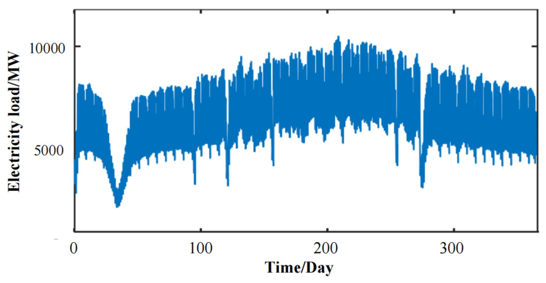
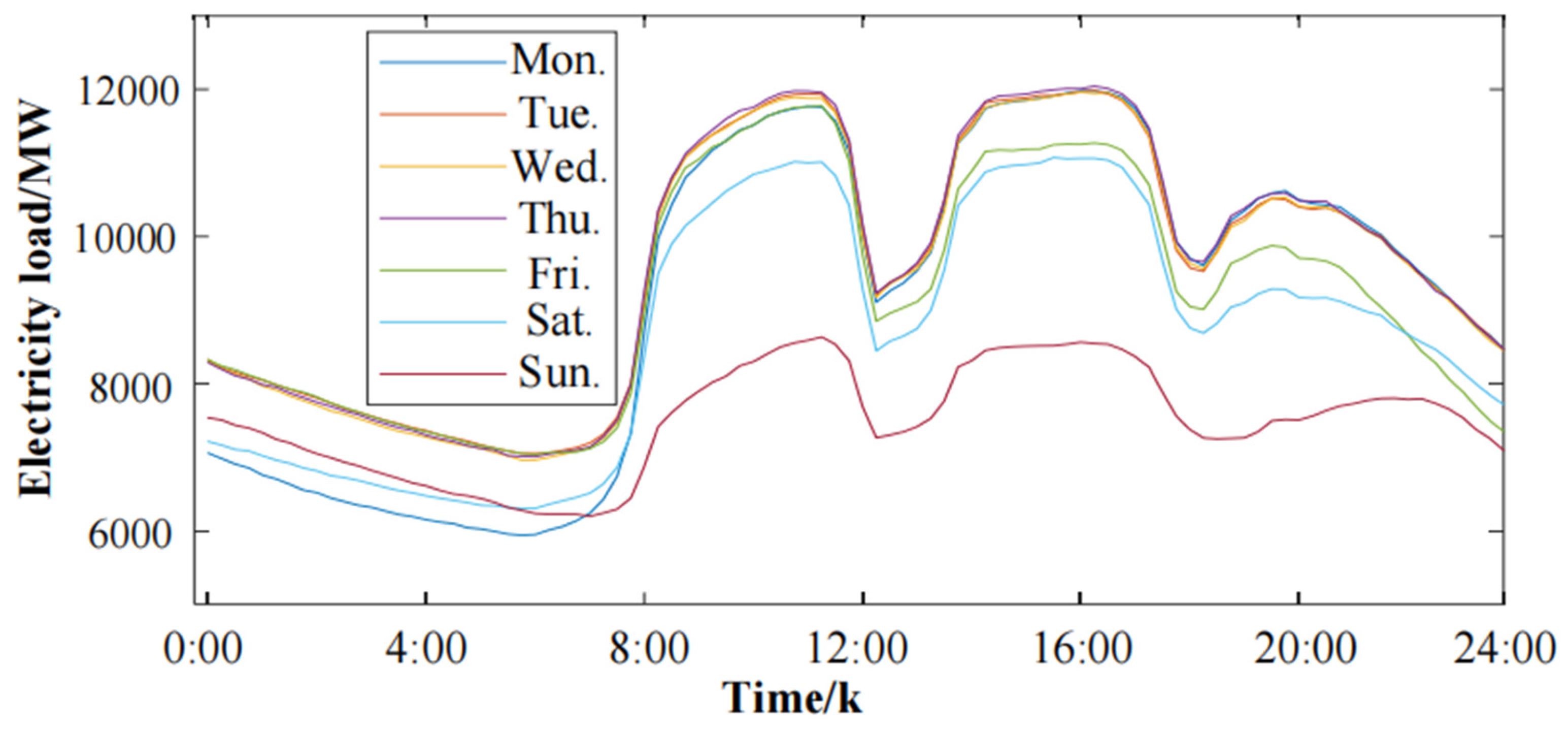
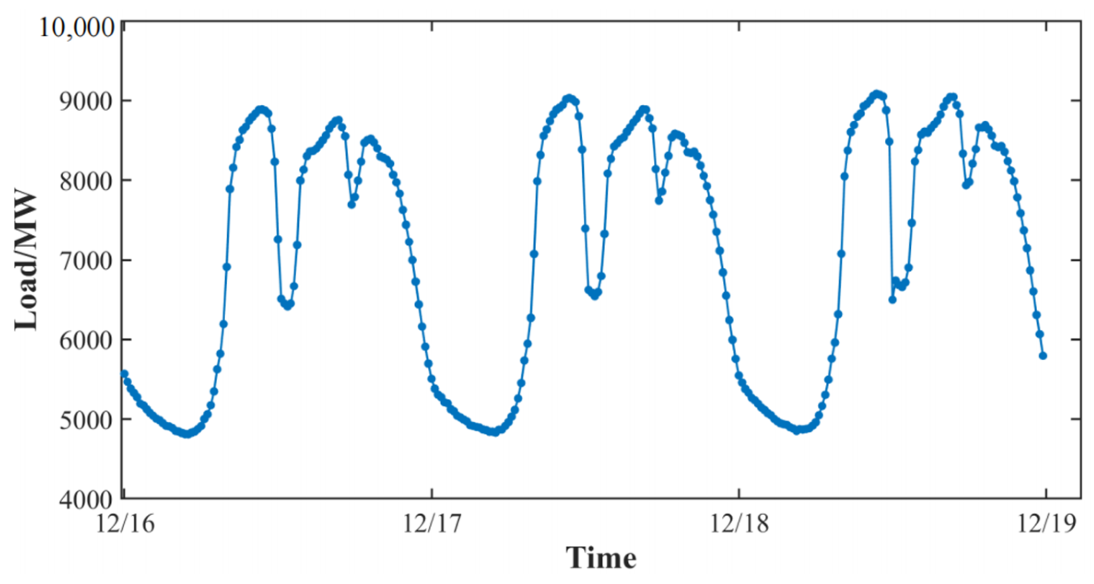
To reflect different influencing factors of power load, this paper conducts an in-depth analysis of the historical load characteristics of a region in North China based on different time dimensions. The load in North China has obvious annual, weekly, daily, and holiday characteristics.

(3)

To facilitate the training of the model network, the multi-source coupling data such as historical load and characteristic weather are normalized, and the date type is quantified by One-Hot encoding. Considering that the mixing of abnormal power load data will seriously affect the accuracy of the load-forecasting model, a similar day-identification method based on grey correlation degree analysis is proposed to identify the close historical load data, and the linear interpolation method is adopted to correct the data, fill in the missing data, and ensure the continuity and consistency of the data. Most of the existing studies directly eliminate the abnormal load data. and will not be corrected.

(4)

Considering that it is difficult to determine parameters such as iteration times and neurons of the LSTM neural network, a load-forecasting modeling method for optimizing LSTM hyperparameters with IPSO is proposed. Linear differential decreasing inertia weights are used to improve the parameter-optimization performance of the basic PSO algorithm and optimize the parameter part of the LSTM neural network. The input data of the model take into account the influence of characteristic weather, date, and historical load data and are compared with the prediction results of other models through case analysis so as to confirm the effectiveness of the proposed model.

This study proposes an IPSO-LSTM model based on the coupling of multiple meteorological factors (such as daily maximum and minimum temperatures, rainfall, air humidity, etc.), historical load data, and date type information. The model optimizes the hyperparameters of LSTM through an improved particle swarm optimization (IPSO) algorithm, significantly enhancing the accuracy and stability of load forecasting. Additionally, it employs grey relational analysis and linear interpolation to handle abnormal load data, ensuring the continuity and consistency of the data. This research fills the gap of traditional load-forecasting methods in dealing with complex meteorological and voltage changes, especially in real-time data updates and complex nonlinear problem processing. Through these innovations, the model provides more accurate load forecasting in complex environments, enhancing its application potential in power grid dispatching and optimization.

2. Load Characteristics Analysis Based on Different Time Dimensions

With the help of multi-source data-coupling technology, the power load data can be collected in real time and accurately, and its variation law can be analyzed deeply. The variation of power load is influenced by numerous factors and presents complex and diverse development laws. Figure 1 illustrates the load curve of a region in North China in 2021 with intensive sensor acquisition (load data interval of 15 min, 96 sampling points per day). As can be seen from the figure, July and August, as midsummer months, have a peak load up to 10,000 MW, and under the influence of hot weather, the temperature control load in the power system occupies a large proportion, and the load level rises significantly compared with the preceding and the following months, showing a significant “peak” feature, accompanied by a large load fluctuation. In December, the cold weather, the special period of rapid economic development of various units and enterprises at the end of the year, the increase in heating load, and the social phenomenon of a large number of production increases work together, making the electricity load also show “peak” characteristics. In January, the load level was significantly reduced, with a minimum of 2000 MW. These data fully show that the load characteristics are closely related to local meteorological conditions.

Figure 2 shows the load curve of a certain week (14 July~20 July) in this area, and the daily electricity load within a week has a certain regularity. At the working day stage, people are in a state of production and life, and the load of office buildings and enterprises is heavier, with a peak load up to 12,000 MW, while the situation is just the opposite on weekends. The minimum load is 7000 MW. Therefore, the load on working days will be slightly higher than that on rest days, and the load has obvious weekly periodicity. To meet the accuracy requirements of load forecasting, the influence of weekly differences should be considered.

Usually, the daily load curve has two peaks, the morning peak and the evening peak; the morning peak is mainly caused by enterprise electricity consumption, and the evening peak is caused by household electricity consumption. Figure 3 shows the typical daily load curve of the region in summer (load data on 1 August, with 96 sampling points). As can be seen from Figure 3, the summer morning peak lasts from about 10:00 to about 18:00, the peak load in the morning peak was 8700 MW, and the evening peak is not obvious. The minimum load at dawn is 4400 MW. This is due to the increase in air conditioning load during the summer, especially around noon during the day.

Considering the influence of important holidays, the load data of the region during and around the National Day in the past four years were taken as an example to analyze the holiday characteristics of the regional load, as shown in Figure 4. The variation trend of power load during National Day in four years is the same; the peak load reaches 8000 MW, and the minimum load is 2200 MW. The load in early October is significantly lower than before the holidays. This is mainly because most industrial and commercial activities are stopped during the holidays, so the impact of holidays on the load is more obvious. When establishing the forecast model, whether the forecast date is a holiday should also be taken into account in the model.

Table 1. Load changes in different time dimensions.

Time Dimension	Peak Load (MW)	Minimum Load (MW)	Load Fluctuation Percentage (%)
year	10,000	4000	150
week	12,000	7000	71.43
day	8500	4500	88.89
Holidays and festivals	8000	2200	263.64

compares the load changes in different time dimensions by peak load, minimum load, and load fluctuation percentage.

According to the above analysis, the general frame diagram of load characteristic analysis in each time dimension is shown in Figure 5.

3. Multi-Source Parameter Coupling Data Processing

Due to the high sensitivity of power load-prediction models to data scales and the large differences in the order of magnitude in the original parameter data of dense sensor coupling, it is essential to limit the input data to a comparable magnitude to prevent the scenario where variations in larger values overshadow those in smaller ones.

3.1. Data Normalization

To facilitate the training of the model network, min-max is used to normalize multi-source data such as historical load and characteristic meteorological data between (−1,1). The formula is as follows:

$$x_{1t}=2\times {\displaystyle \frac{x_t-x_{\min }}{x_{\max }-x_{\min }}}-1$$

(1)

where x_t and x_1t are the actual and normalized values of historical load and characteristic meteorological data at time t, and x_min and x_max are the minimum and maximum values of the data set.

After the prediction is completed, it is necessary to carry out anti-normalization processing of load data. The specific formula is as follows:

$$x_{2t}=(x_{1t}+1)/2\cdot (x_{\max }-x_{\min })+x_{\min }$$

(2)

where, x_2t is the inverse normalized value of the load at time t.

3.2. Date Type Quantization

In this paper, the natural language of date type is converted into data, and One-Hot encoding is adopted to encode it so that different types of dates correspond to one activation code [28,29]. This approach utilizes n—bit status registers to code N states, where each state possesses its independent register bits, and there is only one valid byte at any given time. According to the analysis in Figure 2, the load trends of Tuesdays, Wednesdays, and Thursdays in a working week are close, so the attributes of these three days are combined into one category, and the holidays are Chinese legal holidays such as the Mid-Autumn Festival, National Day, and Dragon Boat Festival (the holidays are the same every year, excluding weekends). The encoding outcomes are presented in

Table 2. Date type quantization.

Date Type		Encoding
Non-holiday	Monday	000001
	Tuesday to Thursday	000010
	Friday	000100
	Saturday	001000
	Sunday	010000
Holidays and festivals		100000

.

The thermal coding method in Table 2 can solve the problem that the predictive model makes it difficult to solve the attribute data, and it does not require decoder operations. Compared with the data quantization method between 0 and 1, the characteristics of the data can be expanded to a certain extent, and the difference between different date types can be more accurately distinguished.

3.3. Abnormal Load Handling

Subject to various factors such as meteorological changes, holidays, emergencies, and power grid equipment failures, power load data often mix with outliers and discontinuous records. When the data volume is large, these irregularities and errors may be expanded, which seriously affects the accuracy of the load-forecasting model. Therefore, the linear interpolation method is used for data correction. Through analyzing the complete load data set, a linear interpolation model is established, and a similar day-identification method is used to identify the close historical load data, fill in the missing data, and ensure the continuity and consistency of the data. In this study, grey relational analysis was used to identify similar days. The specific steps are as follows:

Step 1: The daily maximum temperature, minimum temperature, average temperature, relative precipitation, and humidity are used to identify the reference series, which reflects the characteristics of system behavior, and the comparative series, which influences system behavior. The reference series (parent series) on day i is the data series reflecting the load characteristics of the system on that day and is denoted as F₀; the comparison series (subseries) is a data series composed of factors affecting the load behavior on day i, denoted F_i.

$$F_0=[f_{01},f_{02},\cdots ,f_{0m}]$$

(3)

$$F_i=[f_{i1},f_{i2},\cdots ,f_{im}]$$

(4)

where f_im is the value of the m meteorological factor on the i day (1 ≤ I ≤ I, 1 ≤ m ≤ 5), and I is the sample days in the historical load data set.

Step 2: Obtain the grey correlation coefficient between the parent sequence and the sub-sequence. Its formula is as follows:

$$\left\{\begin{array}{l}{\Delta }_i(m)=\left|f_{0m}-f_{im}\right|\\ {\xi }_i(m)={\displaystyle \frac{\underset{i}{\min } \underset{k}{\min } {\Delta }_i(m)+\rho \underset{i}{\max } \underset{k}{\max } {\Delta }_i(m)}{{\Delta }_i(m)+\rho \underset{i}{\max } \underset{k}{\max } {\Delta }_i(m)}}\end{array}\right.$$

(5)

where ξ_i(m) is the calculated grey correlation coefficient, ρ∈(0, ∞) is called the resolution coefficient, and the value is usually between 0 and 1. Generally, the resolution is best when ρ < 0.5463; ρ = 0.5 is taken in this paper.

Step 3: Consider the correlation degree between the comparison series F_i and the reference series F₀ on various meteorological factors, quantify the correlation degree by obtaining the average of the correlation coefficient, and use the following equal-weight correlation degree formula to determine the correlation extent between the day to be found and day i.

$$r_i={\displaystyle \frac{1}{5}}{\displaystyle \sum _{m=1}^5{\xi }_i(m)}$$

(6)

Since different meteorological factors have different degrees of influence on the load, the weighted correlation degree is introduced for calculation:

$$r_i={\displaystyle \frac{1}{5}}{\displaystyle \sum _{m=1}^5{w}_i{\xi }_i(m)}$$

(7)

where w_i is the weight of daily load, which is calculated using the method of literature [28,29].

Step 4: Rank the correlation degree from large to small. The higher the correlation degree ranking on a certain day, the higher the similarity between the factors affecting the load on that day and the predicted day, and the stronger the correlation of the load. The result is combined with the corresponding date-type coded data to sort the similarity again, and the date with the top ranking is selected as the similar day to be sought.

If the load value at a particular moment is closely related to the load before and after the time, it is similar to the data at that time on similar days; therefore, the abnormal data are filled in by the interpolation method, and the formula is as follows:

$$\left\{\begin{array}{l}{x}_{(d,k)}=a_1{x}_{(d,k-1)}+a_2{x}_{(d,k+1)}+a_3{x}_{(d-1,k)}+a_4{x}_{(d+1,k)}\\ a_n=r_n/{\displaystyle {\sum }_1^n{r}_i}\end{array}\right.$$

(8)

where x_(d, k), x_(d, k−1), and x_(d, k+1) are the load values at k time and before and after the d day, respectively, x_(d−1, k) and x_(d+1, k) are the load values at k time of the two similar days before and after the identification, and a₁, a₂, a_3, and a₄ are the weight coefficients.

4. Regional Power Grid Load-Forecasting Model Based on IPSO-LSTM

Based on the above analysis of load characteristics and main influencing factors, the load-forecasting architecture shown in Figure 6 is established. The essence of load forecasting is a problem about time series forecasting. Generally, the time data before and after time series problems have a certain correlation, and the multi-source data of dense sensor coupling are fused together as the input of the model.

4.1. IPSO-LSTM Load-Forecasting Model

LSTM is an extended neural network proposed on the basis of the defects of standard RNN neural network, as shown in Figure 7. It adds a “processor” that can judge the function of signals. Each processor consists of three gates, namely, the forgetting gate, the input gate, and the output gate [30,31]. The input signals are processed by the sigmoid function.

Considering that the LSTM model is capable of effectively dealing with long-term dependency relationships and capturing the nonlinear features of power load, this paper selects the LSTM neural network for predicting the power load of the regional power grid [32,33,34] and adopts the Adam method for network training to avoid the issues arising from gradient descent. Five characteristic meteorological factors, including daily maximum temperature, daily minimum temperature, average temperature, relative precipitation, and humidity, as well as date and historical load data, were divided into training sets and test sets.

Since various loads of regional power grids have complex and high-dimensional random characteristics, and the number of neurons in the LSTM hidden network is difficult to determine, the number of iterations directly affects the prediction effect. Based on the existing prediction model, the PSO algorithm is introduced to optimize the parameters of LSTM to improve the prediction accuracy of the model [35].

The speed iteration update formula of the particle swarm algorithm with inertial as the particle term at the kth iteration of particle i is as follows [36]:

$$v_{id}^k=w{v}_{id}^{k-1}+c_1{r}_1(pbes{t}_{id}-x_{id}^{k-1})+c_2{r}_2(gbes{t}_d-x_{id}^{k-1})$$

(9)

The position update formula in the dth dimension for particle i is as follows:

$$x_{id}^k=x_{id}^{k-1}+v_{id}^k$$

(10)

where v^k_id and x^k_id are defined as the dth dimensional components of the velocity and position vectors of particle i at the kth iteration, respectively; w is the inertia weight; c₁, c₂ are the acceleration constants; r₁, r₂ are the two mutually independent random functions with distributions between 0 and 1; pbest is the best point in the history that each particle has found during the search based on its search so far, and gbest is the best point found by all particles in the whole population.

Since optimizing all layer parameters will greatly increase the computational complexity and training time, optimizing hidden layer parameters first can balance the performance improvement and computational cost. Therefore, PSO is often used to adjust the hyperparameters that affect the structure of the hidden layer and the training process, without fine-tuning the weight and bias of each layer. The PSO algorithm is used to optimize the hidden layer parameters of the LSTM model to consider the randomness of structural parameters and realize the organic combination of power load prediction and neural network model. The input vector expression is as follows:

$$x\left(t\right)=\left[M(t),D(t),L(t)\right]$$

(11)

$$M(t)=[DMAXTD(t),DMINT(t),DMT(t),DR(t),AH(t)]$$

(12)

where x(t) is the input parameter of the LSTM model; M(t) is the characteristic meteorological factor, including DMATD(maximum daily temperature), DMINT(minimum daily temperature), DMT(average temperature), DR(relative precipitation), and AH(humidity); D(t) is the date type; and L(t) is the historical load data. The LSTM network model based on the deep neural network includes a hidden network. Characteristic meteorological factors, date types, and historical load data are used as input parameters of the PSO-LSTM network structure, which are denoted as follows:

$$x=[M_1^1,M_2^2,\dots ,M_B^K,D_1^1,D_2^2,\dots ,D_B^N,L_1^1,L_2^2,\dots ,L_B^R]$$

(13)

where K, N, and R are the number of characteristic meteorological factors, the number of date types, and the number of historical load samples in the load-forecasting system, respectively.

Sample points A to B are selected as the test set, and the sample before A is the training set. Based on the training set, the PSO-LSTM network model is trained. The specific expression is shown as follows:

$$X_{train}=\left[\begin{array}{cccccccccccc}{M}_1^1& M_1^2& \cdots & M_1^K& D_1^1& D_1^2& \cdots & D_1^N& L_1^1& L_1^2& \cdots & L_1^R\\ M_2^1& M_2^2& \cdots & M_2^K& D_2^1& D_2^2& \cdots & D_2^N& L_2^1& L_2^2& \cdots & L_2^R\\ ⋮& ⋮& \ddots & ⋮& ⋮& ⋮& \ddots & ⋮& ⋮& ⋮& \ddots & ⋮\\ M_A^1& M_A^2& \cdots & M_A^K& D_A^1& D_A^2& \cdots & D_A^N& L_A^1& L_A^2& \cdots & L_A^R\end{array}\right]$$

(14)

$$Y_{train}={\left[\begin{array}{cccc}{\beta }_1& {\beta }_2& \cdots & {\beta }_A\end{array}\right]}^{\mathrm{T}}$$

(15)

$$X_{test}=\left[\begin{array}{ccccccccc}{M}_{B-A}^1& \cdots & M_{B-A}^K& D_{B-A}^1& \cdots & D_{B-A}^N& L_{B-A}^1& \cdots & L_{B-A}^R\\ M_{B-A+1}^1& \cdots & M_{B-A+1}^K& D_{B-A+1}^1& \cdots & D_{B-A+1}^N& L_{B-A+1}^1& \cdots & L_{B-A+1}^R\\ ⋮& \ddots & ⋮& ⋮& \ddots & ⋮& ⋮& \ddots & ⋮\\ M_B^1& \cdots & M_B^K& D_B^1& \cdots & D_B^N& L_B^1& \cdots & L_B^R\end{array}\right]$$

(16)

$$Y_{test}={\left[\begin{array}{cccc}{\beta }_{B-A}& {\beta }_{B-A+1}& \cdots & {\beta }_B\end{array}\right]}^{\mathrm{T}}$$

(17)

where B is the total number of input sample points of the neural network; A is the number of sample points in the training set of the neural network; and Y is the result of regional power grid load-prediction output by a neural network.

Considering that the previously time-invariant acceleration coefficient will weaken the global search ability and convergence speed of particles, and it is easy to fall into the local optimal prematurely, this paper constructs the IPSO algorithm with linear differential decreasing weights of time-varying acceleration constants to further optimize the parameters of the LSTM neural network, and the population sensitivity is defined as follows [37]:

$$\left\{\begin{array}{ll}k(g)=1& g=1\\ k(g)={\displaystyle \frac{StdFit(g)}{StdFit(g-1)}}& g>1\end{array}\right.$$

(18)

where g is the current number of iterations and StdFit(g) is the standard deviation of the fitness of the population in generation g. At the beginning of the iteration, the range of fluctuation of k(g) is small, and the weight factor decreases smoothly, and at the later stage of the iteration there is a strong convergence of the population, and the range of fluctuation of k(g) is strong.

The Sigmoid function is utilized to construct the neuron activation function with the expression:

$$S(x)={\displaystyle \frac{1}{1+\exp (-x)}}$$

(19)

Joint evolutionary discretization k(g) and Sigmoid function are used to construct time-varying acceleration constant linear differential decreasing weights:

$$w(g)=w_{\max }-(w_{\min }-w_{\max }){\displaystyle \frac{1}{1+\exp \left[-10b\left(\frac{2g}{k(g)·G}-1\right)\right]}}$$

(20)

where w_max is the maximum weight; w_min is the minimum weight; b is the damping factor; and G is the maximum number of iterations.

The specific steps for solving the load forecast are as follows:

• Step 1: Multi-source data such as characteristic meteorological data and historical load are normalized, and date types are encoded by One-Hot technology to get a reasonable input between 0–1.
• Step 2: The grey relational analysis method is used to calculate similar days, and the linear interpolation method is used to correct abnormal historical load data.
• Step 3: Split the sample data into a training set and a testing set.
• Step 4: Initialization of model parameters: set the evolution number N_gen, population size sizepop, acceleration factors c₁ and c₂, limits of particle velocity and position values V_min, V_max, popmin, popmax, and maximum and minimum values of inertia weights w_max and w_min.
• Step 5: Randomly generate the initial particle population pop₀(h, ε), where h corresponds to the number of neurons in the hidden layer and ε corresponds to the learning rate; randomly generate the initial velocity V₀ of the particles, which corresponds to the velocities of the two important hyperparameters.
• Step 6: Select the evaluation function of the particles. The particles obtained in Step 5 are assigned to the hyperparameters of the LSTM network correspondingly. Input training samples for LSTM training, training to the maximum number of iterations of the LSTM when the termination of training, to obtain the output value of the training samples; in this paper, the mean square error MSE is selected as the evaluation function of the fitness.
• Step 7: Calculate the fitness value of each particle, take the particle value corresponding to the historical best fitness of each particle as the individual best particle p_best for each particle, and instead of the current particle position, select the particle with the smallest fitness as the group best particle gbest iteration.
• Step 8: After starting the next iteration, update the inertia weights and learning factors, and update the position and velocity of each particle. At this time, to avoid the particle swarm algorithm falling into the local optimum, a single particle random variation is added. Update the fitness of the population and repeat Step 7.
• Step 9: After reaching the maximum number of evolutions of the particle swarm, N_gen, or the value of the fitness, reaches stability, the particle updating iteration is stopped, and the optimal training result of the final gbest is obtained.
• Step 10: Assign the values of the gbest particles correspondingly to the LSTM, import the inputs from the training set into the IPSO-LSTM prediction model for iterative model optimization, and choose the Adam optimization method for the network training method.
• Step 11: The inputs of the test set are imported into the trained prediction model in Step 10 to calculate the predicted outputs, the predicted output loads are inverted normalized to obtain the predicted load truth values, and the expected outputs of the test set are used to calculate the model evaluation indexes and complete the load prediction.

The specific modeling process is shown in Figure 8.

4.2. IPSO Performance Verification

To show the overall performance of IPSO more intuitively, the IPSO algorithm is compared with other improved PSO algorithms such as CW-PSO, CLDIW-PSO, and (tan, sin)CNIW-PSO algorithm. The parameters are set as follows: The number of particles in PSO is 40, the dimension of each particle is 30, and the number of iterations is 1000. The green line represents the performance of CW-PSO, the red line represents the performance of CLDIW-PSO, the purple and blue lines represent the performance of two (tan, sin)CNIW-PSO, and the black line represents the performance of IPSO. The test function is shown in Equation (21). The optimal value of the function is presented in

Table 3. Test the optimal value of the function.

Function Name	Optimal Value
Ackley function	(0, 0)
Griewank function	(0, 0, 0)
Rastrigin function	(0, 0)
Schaffer function	Multiple locally optimal solutions
Sphere function	(0, 0)
Rosenbrock function	(1, 1, 0)

, while the calculation results are illustrated in Figure 9.

$$\left\{\begin{array}{l}{F}_1=-20e^{-0.2\sqrt{{\displaystyle \frac{{\displaystyle {\sum }_{g=1}^G{x}_g^2}}{G}}}}-e^{{\displaystyle \frac{{\displaystyle {\sum }_{g=1}^G\cos (2\pi x_g)}}{G}}}+22.71282\\ F_2=1+{\displaystyle \frac{1}{4000}}{\displaystyle \sum _{g=1}^G{x}_g^2}-{\displaystyle \prod _{g=1}^G\cos \left(\frac{x_g}{\sqrt{g}}\right)}\\ F_3=10G+{\displaystyle \sum _{g=1}^G\left[x_g^2-10\cos \left(2\pi x_g\right)\right]}\\ F_4=0.5+{\displaystyle \frac{{\sin }^2\left(x_1^2-x_2^2\right)-0.5}{\left[1+0.001\left(\left(x_1^2+x_2^2\right)\right)\right]}}\\ F_5={\displaystyle \sum _{g=1}^G{x}_g^2}\\ F_6={\displaystyle \sum _{g=1}^{G-1}\left[{\left(1-x_g\right)}^2+100{\left(x_{g+1}-x_g^2\right)}^2\right]}\end{array}\right.$$

(21)

where F₁ is the Ackley function value, F₂ is the Griewank function value, F₃ is the Rastrigin function value, F₄ is the Schaffer function value, F₅ is the Sphere function value, F₆ is the Rosenbrock function value, and x_g is the function value of the g iteration. x_g−1 is the function value of the g − 1 iteration, and G is the number of iterations.

As can be seen from Figure 9, the CW-PSO method has a better test performance only on the Rosenbrock function, the CLDIW-PSO method has a better performance in the Griewank function but an average performance in the optimization search process for the other functions, and the tangent method of the two CNIW-PSO methods does not have as good a performance as the sinusoidal method in the Rastrigin function, but the opposite is true in the Griewank function. While the performance of both of them is just in the middle level, the IPSO method basically reaches the lowest fitness function in Sphere, Rastrigin, Schaffer, and Ackley functions, and the performance in Griewank and Rosenbrock is also in the middle level, and collectively, the convergence performance of the IPSO method is better.

4.3. Model Evaluation Criteria

To accurately appraise the prediction performance of the IPSO-LSTM network model put forward in this paper, mean relative error (MAPE), root mean square error (RMSE), and mean absolute error (MAE) were adopted as evaluation indicators to analyze the model’s prediction result. The smaller the values of MAPE, RMSE, and MAE, the greater the goodness of fit. The more accurate the model prediction results are, the precise definition formula is given as follows:

$$E_{\mathrm{MAPE}}={\displaystyle \frac{1}{N}}{\displaystyle \sum _{k=1}^N\left|\frac{y_{act}(k)-y_{pred}(k)}{y_{act}(k)}\right|}$$

(22)

$$E_{\mathrm{RMSE}}=\sqrt{{\displaystyle \frac{1}{N}}{\displaystyle \sum _{k=1}^N{\left(y_{act}(k)-y_{pred}(k)\right)}^2}}$$

(23)

$$E_{\mathrm{MAE}}={\displaystyle \frac{{\displaystyle \sum _{k=1}^N\left|y_{act}(k)-y_{pred}(k)\right|}}{N}}$$

(24)

where N represents the sample size of the test set and y_act(k) and y_pred(k) (k = 1, 2, …, N) are the real value and predicted value of the regional load at time k, respectively.

5. Calculus Analysis

In order to verify the reliability and scientificity of the IPSO-optimized LSTM neural network algorithm proposed in this paper for short-term power load forecasting, the load data of dense sensor coupling in a region of North China was taken as an example and calculated by MATLAB2020a software.

5.1. Data Preprocessing

The 24-h weather data of 18 December were selected for load forecasting, but the abnormal data at noon on 18 December were identified based on the historical load data. The abnormal load is shown in the red part of Figure 10, and the abnormal data should be corrected using a similar day method.

To find similar days to 18 December (Thursday), meteorological factors and load data of the 10 days before and after the selection (8 December to 28 December) need to be normalized, as shown in

Table 4. Data sample of influence factors after normalization.

Date	Raw Data					Normalized Data After Processing
	DMAXT	DMINT	DMT	DR	AH	DMAXT	DMINT	DMT	DR	AH
12.8	19.6	11.9	14.9	81	3.2	0.65	0.51	0.46	0.79	0.29
12.9	22.7	15.4	18.2	64	0	0.96	0.91	0.86	0.56	0
…	…	…	…	…	…	…	…	…	…	…
12.18	14.5	7.9	11.2	35	0	0.14	0.045	0.023	0.15	0
…	…	…	…	…	…	…	…	…	…	…
12.27	16	13.2	14.3	96	11	0.29	0.66	0.39	1	1
12.28	14.5	11	12.6	87	4.8	0.14	0.40	0.19	0.87	0.43

.

With the quantity of the main influencing factors of that day as the parent sequence and the influencing factors data of other days as their respective sub-sequences, the correlation degree of influencing factors calculated by GRA theory is shown in Figure 11.

It can be seen from Figure 11 that the days with higher similarity are the 10th, 15th, 6th, 16th, 13th, etc. After adding the date type encoded by One-Hot, the two similar days before and after are identified as 17 December and 23 December. The abnormal data are corrected by using the load data of the same time before and after the two similar days and the load data of the same time before and after the day, in which the weight coefficient of each load is 1/4. The corrected data are shown in Figure 12. Finally, the completed and corrected load data were normalized, and the data after processing were shown in

Table 5. Sample of processed power load data (take 12.16–12.18 as an example).

Time	Raw Data (MW)			Normalized Data After Processing
	12.16	12.17	12.18	12.16	12.17	12.18
0:00	5570	5506	5549	0.177	0.163	0.173
0:15	5469	5388	5459	0.153	0.138	0.152
0:30	5384	5308	5379	0.134	0.116	0.132
…	…	…	…	…	…	…
23:45	5910	5995	6066	0.257	0.277	0.294
24:00	5697	5756	5795	0.207	0.221	0.230

, so that the pre-processing of 24-h meteorological factors and load and other related data on 18 December was completed.

5.2. LSTM Parameter Determination and IPSO Optimization

The number of neurons in each layer of the neural network is determined based on the input-output model within the forecasting framework proposed in this paper. The prediction model takes 96-dimensional historical load data, 5-dimensional weather data, and 6-dimensional thermally encoded date-type data as its input, and its output is 96-dimensional load values for one day in the future. Consequently, the input layer of this network has 107 nodes. Since the output of the prediction model is 96-dimensional load data for one day, the number of nodes in the output layer is 96. The number of nodes in the hidden layer is obtained through the improved particle swarm algorithm. The specific parameters of the particle swarm algorithm with linear differential decreasing weights are set as follows: the population size is 40, the dimension of each particle is 2, and the number of evolutionary iterations, N_gen, is set to 100. The inertia weight ranges from 0.4 to 0.9, and the learning factors c₁ and c₂ have a range of [0, 2], which are updated once per iteration. The value range of the particle pop₀(h, ε) element is set to [1, 100] and [0.0001, 0.01], respectively, and the velocity range of the particle is [−5, 5] and [0.0004, 0.0006].

The data from the dataset after preprocessing for the whole year are divided into a training set and a test set. The training set samples are utilized to obtain the optimization search results for the two hyperparameters h, ε of the LSTM. From Figure 13a, it can be seen that the fitness can be stabilized around 0.041 eventually as the number of iterations of the particle swarm increases. Figure 13b shows that the number of neurons in the hidden layer is stabilized at 15, and Figure 13c shows that the learning rate is stabilized around 0.005 eventually as the number of iterations increases.

The aforementioned results were input into the prediction model, and the Adam method was employed for the iterative training of the LSTM neural network. The initial 90% of the sequence was utilized for training in order to acquire the optimal weight and threshold, while the remaining 10% of the data served as a test set for testing purposes. The architecture of the neural network model with LSTM is 107 × 15 × 96, and the learning rate is set at 0.005. In contrast, the BP neural network structure is 107 × 22 × 96, with a learning rate of 0.0009. Furthermore, the constructed Elman neural network has a structure of 107 × 13 × 13 × 96, a learning rate of 0.004, and a total number of iterations amounting to 500. The actual load curve of a specific day in the test set along with the prediction curves of the three different models are depicted in Figure 14. The relative errors of various methods at different times are illustrated in Figure 15. Lastly, the calculation results are presented in

Table 6. Comparison of prediction error metrics of different models.

	MAPE/%	RMSE	MAE
IPSO-BP	2.6549	234.2583	192.7381
IPSO-Elman	1.2139	115.6638	86.1528
IPSO-LSTM	0.8840	80.1699	62.0612

.

Combined with the findings presented in Figure 14 and Figure 15, as well as Table 6, it is evident that the forecast trajectories of the three models align with the actual value fluctuations to a noticeable degree. This suggests that the load-forecasting framework developed in this study is, to a significant extent, rational and capable of capturing the load variation patterns effectively. However, a closer examination reveals that the optimized BP neural network exhibits the poorest predictive accuracy, primarily due to its lack of a memory mechanism, which results in substantial errors at intervals with significant load variations. While the optimized Elman neural network shows an enhanced predictive capability compared to the BP model, it still encounters sizable errors at certain instances. The IPSO-LSTM neural network introduced in this paper outperforms both the BP and Elman models, with a reduction in the MAPE by 1.8149% and 0.3299%, respectively, a decrease in the RMSE by 154.0884 and 35.4939, and a reduction in the MAE by 130.6769 and 24.0916, respectively. Ultimately, the IPSO-LSTM model demonstrates a commendable performance in addressing the load-forecasting challenge of this time series, with approximately 91.67% of the error points falling within a 2% margin.

Compared with some load-forecasting methods in literature, the calculation results are shown in the

Table 7. Comparison of different load-forecasting methods.

	MAPE/%	RMSE	MAE
Multivariate Linear Regression	3.21	280.34	220.12
Support Vector Regression	2.98	256.78	201.34
IPSO-LSTM	0.8840	80.1699	62.0612

.

From the above comparison results, it can be clearly seen that under the same test data set and evaluation indicators, the IPSO-LSTM method proposed in this paper has significant advantages in prediction accuracy compared with traditional multivariate linear regression and support vector regression methods. Due to its assumption of the linear relationship of data, multivariable linear regression has a large error when dealing with complex nonlinear data such as power load. Although support vector regression can deal with nonlinear problems to a certain extent, its prediction performance is still inferior to the IPSO-LSTM model when facing multi-source parameter coupling and complex time series data involved in this paper.

Taking into account the distinct seasonal variations in power demand throughout the year, the IPSO-optimized LSTM neural network was employed to predict the load for representative days across the four seasons of 2021, in order to further validate the model’s forecasting accuracy. Following the selection criteria outlined in reference [38], the days chosen to represent each season were 10 March, 18 June, 6 October, and 3 December. The outcomes of these predictions are depicted in Figure 16, while the corresponding error metrics are detailed in

Table 8. Comparison of forecast error indicators for a day in four seasons.

Typical Day	MAPE/%	RMSE	MAE	Percentage of Error < 2%
10 March	0.87	83.9343	58.7613	90.63
18 June	0.95	74.6874	89.7552	90.63
6 October	0.71	86.4276	55.4041	93.75
3 December	0.78	64.2497	55.0478	92.17

.

As can be seen from the results of Figure 16 and Table 8, in the prediction of typical days in different seasons, this method can keep the relative error of more than 90% of the sampling points below 2%, and the relative error of the square pair is basically below 1%, and the value of the root-mean-square error and the average absolute error account for a small proportion of the daily base load level. The above results indicate that this model has relatively good applicability.

From the above calculation results, it can be seen that the proposed IPSO-LSTM model shows high accuracy and stability in the overall load prediction. Compared with other models, its advantages are obvious. When dealing with load data with complex change rules, such as load difference between weekdays and weekends, load fluctuation in different seasons, etc., the IPSO-LSTM model can better capture data characteristics, which is due to the effective processing ability of LSTM network for long-term dependence relations and the optimization of model parameters by IPSO algorithm. For example, during the peak of electricity consumption in summer and the peak of heating load in winter, the model can still maintain a low prediction error, indicating that it has a good adaptability to seasonal load changes.

However, there are some improvements to the model. In the case of sudden load changes caused by some special weather mutations or unexpected events, although the model can reflect the load change trend to a certain extent, the prediction error will still increase, which may be due to the relatively small number of samples in the training data set for such extreme situations, and the model is not sufficiently learned.

In terms of load forecasting in peacetime and holidays, the model’s forecasting performance in peacetime is relatively stable and accurate, and the relative error of most sampling points can be controlled at a low level because the load change law in peacetime is relatively stable, and the model can better capture its periodicity and trend by learning historical data. During holidays, although the model has taken into account the holiday factor, the accuracy of the model prediction is slightly decreased compared with normal times due to the differences in social activities and economic operation during holidays in different years. For example, in long holidays such as the National Day, the time point and degree of stoppage of some industrial and commercial activities may not be exactly the same every year, which brings certain challenges to the model prediction. But in general, through the quantification of date types and the comprehensive consideration of related factors, the model still has reference value in the forecast results of holidays.

6. Conclusions

This study introduces a novel approach for short-term load forecasting in the IPSO-LSTM domain, which accounts for the interplay of various parameters. It utilizes actual load data from a northern Chinese region to perform computations and validate the model’s effectiveness. The following conclusions can be drawn from the analysis of this paper:

(1)

The model prediction framework established in this paper is reasonable. Considering more comprehensive multi-source influencing factors as model input, using One-Hot coding to represent the date type with 6-bit register bits, expanding the data feature dimension, and calculating similar days by grey relational analysis can well correct the abnormal load, laying a foundation for the accuracy of the prediction model.

(2)

After preprocessing the multi-source parameter data of dense sensor coupling, the IPSO algorithm is used to optimize and solve the important parameters in the LSTM model. Tests are carried out on six commonly used standard test functions, and it is verified that the PSO algorithm with linear differential decreasing inertia weight has good convergence and optimization ability. The problem of selecting the initial parameters of standard LSTM is solved effectively.

(3)

The IPSO-optimized LSTM neural network model established in this paper can keep the relative error of more than 90% of the sampling points below 2%, and the short-term power load prediction results at different times are close to the actual load. Meanwhile, compared with other models in power load prediction, it has higher accuracy and stability and lower error, and it has certain practical application potential.

(4)

In practical applications, the power grid load is affected by a variety of complex factors, and the load characteristics in different scenarios may be quite different. Whether the IPSO-optimized LSTM neural network model established in this paper can adapt to these differences and maintain good prediction performance needs to be further tested and verified on a wider dataset. In the future, load data from different regions and different types of power grids can be collected and integrated to build more comprehensive and diverse data sets. By training and validating the model on these datasets, the generalization ability of the model can be improved, so that it can better adapt to the requirements of load forecasting in various complex scenarios.

References

1. Lisardo, P.G.; Anna, F.; Juan, M.G.B.; Angela, P.; Antonio, d.A.S. A Survey on Energy Efficiency in Smart Homes and Smart Grids. Energies 2021, 14, 7273. [Google Scholar] [CrossRef]
2. Chen, J.; Liu, L.; Guo, K.; Liu, S.; He, D. Short-Term Electricity Load Forecasting Based on Improved Data Decomposition and Hybrid Deep-Learning Models. Appl. Sci. 2024, 17, 5966. [Google Scholar] [CrossRef]
3. Liao, Y.; Weng, Y.; Tan, C.W.; Rajagopal, R. Quick Line Outage Identification in Urban Distribution Grids via Smart Meters. CSEE J. Power Energy Syst. 2022, 8, 1074–1086. [Google Scholar]
4. Alhamrouni, I.; Kahar, H.A.; Salem, M.; Swadi, M.; Zahroui, Y.; Kadhim, D.J.; Mohamed, F.A.; Nazari, M.A. A Comprehensive Review on the Role of Artificial Intelligence in Power System Stability, Control, and Protection: Insights and Future Directions. Appl. Sci. 2024, 14, 6214. [Google Scholar] [CrossRef]
5. Liu, Y.; Du, W.; Xiao, L.; Wang, H.; Bu, S.; Cao, J. Sizing a Hybrid Energy Storage System for Maintaining Power Balance of an Isolated System With High Penetration of Wind Generation. IEEE Trans. Power Syst. 2016, 31, 3267–3275. [Google Scholar] [CrossRef]
6. Li, X. Study on Correlation Between Load and Meteorological Information of Liaoning Power Grid; North China Electric Power University: Beijing, China, 2014. [Google Scholar]
7. Xu, Y.; Zhang, J.; Ji, X.; Wang, B.; Deng, Z. Research on short-term load forecasting method based on multi-model fusion neuralnetwork. Control Eng. 2019, 4, 619–624. [Google Scholar]
8. Zhang, L.; Zhang, T.; Wang, F.; Qi, X. Ultra-short-term forecasting method based on response characteristics of flexible load. Power Syst. Prot. Control 2019, 9, 27–34. [Google Scholar]
9. Shi, J.; Zhang, J. Load forecasting based on multi model by Stacking ensemble learning. Proc. CSEE 2019, 14, 4032–4042. [Google Scholar]
10. Chen, H.; Wang, S.; Wang, S.; Wang, D. Aggregated load forecasting method based on gated recurrent unit networks and model fusion. Autom. Electr. Power Syst. 2019, 43, 65–74. [Google Scholar]
11. Liu, X.; Lin, Z.; Feng, Z. Short-term offshore wind speed forecast by seasonal ARIMA-A comparison against GRU and LSTM. Energy 2021, 227, 120492. [Google Scholar] [CrossRef]
12. Chen, H.; Yang, Y.; Zhang, R. Study on Electric Power Steering System Based on ADAMS. Procedia Eng. 2011, 15, 474–478. [Google Scholar] [CrossRef]
13. Fan, C.; Guo, Y. Design of the Auto Electric Power Steering System Controller. Procedia Eng. 2012, 29, 3200–3206. [Google Scholar]
14. Paparoditis, E.; Sapatinas, T. Short-Term Load Forecasting: The Similar Shape Functional Time Series Predictor. IEEE Trans. Power Syst. 2013, 28, 3818–3825. [Google Scholar] [CrossRef]
15. Lei, S.; Sun, X.; Zhou, Q.; Zhang, X. Research on multivariate time series linear regression forecasting method for short-term load of electricity. Proc. CSEE 2006, 1, 27–31. [Google Scholar]
16. Song, K.; Ha, S.; Park, J.W. Hybrid load forecasting method with analysis of temperature sensitivities. IEEE Trans. Power Syst. 2006, 21, 869–876. [Google Scholar] [CrossRef]
17. Rafiei, M.; Niknam, T.; Aghaei, J. Probabilistic Load Forecasting using an Improved Wavelet Neural Network Trained by Generalized Extreme Learning Machine. IEEE Trans. Smart Grid 2018, 9, 6961–6971. [Google Scholar] [CrossRef]
18. Ko, C.; Lee, C. Short-term load forecasting using SVR (support vector regression)-based radial basis function neural network with dual extended Kalman filter. Energy 2013, 49, 413–422. [Google Scholar] [CrossRef]
19. Reddy, S.S.; Jung, C.M. Short-term load forecasting using artificial neural networks and wavelet transform. Int. J. Appl. Eng. Res. 2016, 11, 9831–9836. [Google Scholar]
20. Din, G.M.U.; Marnerides, A.K. Short term power load forecasting using Deep Neural Networks. In Proceedings of the 2017 International Conference on Computing, Networking and Communications (ICNC), Silicon Valley, CA, USA, 26–29 January 2017; pp. 594–598. [Google Scholar]
21. Liang, Y.; Niu, D.; Hong, W. Short term load forecasting based on feature extraction and improved general regression neural network model. Energy 2019, 166, 653–663. [Google Scholar] [CrossRef]
22. Zhao, Z.; Huang, W.; Wei, Y. A medium and long-term power load forecasting method based on wavelet analysis and Elman dynamic neural network. Shanxi Electr. Power 2013, 1, 1–5. [Google Scholar]
23. Zhou, H.; Dou, Z.; Zhang, B.; Zhu, Y.; Liao, Q.; Sun, K. Short-term load forecasting based on boosted wavelets and improved PSO-Elman neural network. Electr. Meas. Instrum. 2020, 57, 119–125. [Google Scholar]
24. Kong, W.; Dong, Z.; Jia, Y.; David, J.H.; Xu, Y.; Zhang, Y. Short-Term Residential Load Forecasting Based on LSTM Recurrent Neural Network. IEEE Trans. Smart Grid 2019, 10, 841–851. [Google Scholar] [CrossRef]
25. Tan, M.; Yuan, S.; Li, S.; Su, Y.; Li, H.; He, F. Ultra-Short-Term Industrial Power Demand Forecasting Using LSTM Based Hybrid Ensemble Learning. IEEE Trans. Power Syst. 2020, 35, 2937–2948. [Google Scholar] [CrossRef]
26. Stefan, U.; Vasile, T.; Andrei, C.C. Analysis for Non-Residential Short-Term Load Forecasting Using Machine Learning and Statistical Methods with Financial Impact on the Power Market. Energies 2021, 14, 6966. [Google Scholar] [CrossRef]
27. Wei, T.; Pan, T. Short-term power load forecasting based on improved PSO optimized LSTM network. J. Syst. Simul. 2021, 4, 1–8. [Google Scholar]
28. Ge, Z.; Liu, Y. Analytic Hierarchy Process Based Fuzzy Decision Fusion System for Model Prioritization and Process Monitoring Application. IEEE Trans. Ind. Inform. 2019, 15, 357–365. [Google Scholar] [CrossRef]
29. Huang, T.D.; Shao, Z.D. An evidential network approach to reliability assessment by aggregating system-level imprecise knowledge. Qual. Reliab. Eng. Int. 2023, 39, 1863–1877. [Google Scholar] [CrossRef]
30. Masood, Z.; Gantassi, R.; Choi, Y. Enhancing Short-Term Electric Load Forecasting for Households Using Quantile LSTM and Clustering-Based Probabilistic Approach. IEEE Access 2024, 12, 77257–77268. [Google Scholar] [CrossRef]
31. Liu, Y.; Liang, Z.; Li, X. Enhancing Short-Term Power Load Forecasting for Industrial and Commercial Buildings: A Hybrid Approach Using TimeGAN, CNN, and LSTM. IEEE Open J. Ind. Electron. Soc. 2023, 4, 451–462. [Google Scholar] [CrossRef]
32. Kwang, H.K.; Byunghoon, C.; Kyu, C.H. Deep Learning Based Short-Term Electric Load Forecasting Models using One-Hot Encoding. J. IKEEE 2019, 23, 852–857. [Google Scholar]
33. Wang, C.; Han, D.; Liu, Q.; Luo, S. A Deep Learning Approach for Credit Scoring of Peer-to-Peer Lending Using Attention Mechanism LSTM. IEEE Access 2019, 7, 2161–2168. [Google Scholar] [CrossRef]
34. Ma, J.; Liu, H.; Peng, C.; Qiu, T. Unauthorized Broadcasting Identification: A Deep LSTM Recurrent Learning Approach. IEEE Trans. Instrum. Meas. 2020, 69, 5981–5983. [Google Scholar] [CrossRef]
35. Xie, T.; Zhang, Y.; Zhang, G.; Zhang, K.; Li, H.; He, X. Research on electric vehicle load forecasting considering regional special event characteristics. Front. Energy Res. 2024, 12, 1341246. [Google Scholar] [CrossRef]
36. Yan, H. A Novel Cloud-IPSO-DBN Algorithm for Evaluating Digital Smart City Construction. IEEE Syst. J. 2023, 17, 5109–5117. [Google Scholar] [CrossRef]
37. Wang, S.; Liu, Y. A nonlinear dynamic adaptive inertia weight PSO algorithm. Comput. Simul. 2021, 38, 249–253. [Google Scholar]
38. Li, M.; Cheng, H.; Yang, Z.; Han, X.; Yang, J. Using fractal interpolation prediction method of typical daily load curve of improvement. Proc. CSU-EPSA 2015, 27, 36–41. [Google Scholar]
Figure 1. 2021 load curve of a region in North China.
Energies 18 00516 g001
Figure 2. One week load curve of a region in North China.
Energies 18 00516 g002
Figure 3. Load curve of an area in North China on 1 August.
Energies 18 00516 g003
Figure 4. Load curve of a region in China during four years of National Day.
Energies 18 00516 g004
Figure 5. General frame diagram of load characteristics analysis in different time dimensions.
Energies 18 00516 g005
Figure 6. Multi-source coupled input of load-forecasting model.
Energies 18 00516 g006
Figure 7. Schematic diagram of the internal structure of LSTM. * is the meaning of the product.
Energies 18 00516 g007
Figure 8. Regional power grid load-forecasting model based on IPSO-LSTM.
Energies 18 00516 g008
Figure 9. Iteration curves for five improved POS algorithms.
Energies 18 00516 g009
Figure 10. Abnormal load schematic.
Energies 18 00516 g010
Figure 11. Correlation of load-influencing factors.
Energies 18 00516 g011
Figure 12. Load data after processing.
Energies 18 00516 g012
Figure 13. LSTM hyperparameter training results by IPSO algorithm: (a) Adaptation changes; (b) Variation in the number of neurons in the hidden layer; (c) Learning rate change.
Energies 18 00516 g013aEnergies 18 00516 g013b
Figure 14. Results of different model predictions.
Energies 18 00516 g014
Figure 15. Prediction errors of different models.
Energies 18 00516 g015
Figure 16. Predicted results for the four seasons on a given day: (a) Spring forecast loads and errors; (b) Summer forecast loads and errors; (c) Fall forecast loads and errors; (d) Winter forecast loads and errors.
Energies 18 00516 g016