Article

Multi-Objective Cross-Entropy Approach for Distribution System Reliability Evaluation

by
Lucas Fritzen Venturini
1,2,3,
Beatriz Silveira Buss
1,2,
Erika Pequeno dos Santos
4,
Leonel Magalhães Carvalho
5 and
Diego Issicaba
1,2,*
1
Department of Electrical and Electronics Engineering, Federal University of Santa Catarina, Florianópolis 88040-900, SC, Brazil
2
Institute for Systems and Computer Engineering, Research & Development of Brazil—INESC P&D Brasil, Santos 11055-300, SP, Brazil
3
CELESC Distribuição S.A., Florianópolis 88034-900, SC, Brazil
4
National Service for Industrial Training—SENAI/SC, Florianópolis 88034-001, SC, Brazil
5
Centro Universitário do Porto, Universidade Lusófona, 4000-098 Porto, Portugal
*
Author to whom correspondence should be addressed.
Energies 2025, 18(24), 6421; https://doi.org/10.3390/en18246421
Submission received: 10 September 2025 / Revised: 17 November 2025 / Accepted: 23 November 2025 / Published: 8 December 2025
(This article belongs to the Section F1: Electrical Power System)

Abstract

Reliability evaluation of power distribution systems is computationally intensive, as standard Monte Carlo simulations require extensive sampling to accurately estimate rare event-based indices like SAIDI and SAIFI. This paper introduces a multi-objective cross-entropy approach for reliability evaluation of power distribution systems, aiming to accelerate reliability evaluation by optimizing importance sampling reference parameters. The multi-objective approach aims to optimize a set of objective functions related to systemic and load point reliability indices. A deduction of an analytical solution for the optimization of reference parameters of the cross-entropy method is developed, taking into account the standard hypotheses used in reliability assessments. The proposed method has been validated on a real 181-node Brazilian distribution feeder. Results show that the proposed approach can accelerate the convergence of estimates for reliability indices in comparison with the crude Monte Carlo approach and the single-objective CE method.

1. Introduction

Simulation approaches based on the Monte Carlo method are widely applied in reliability studies and extremely useful for the analysis of large and complex power systems. However, the estimation of reliability indices through simulation approaches may require significant computational time for robust systems. In order to improve the efficiency of the Monte Carlo simulation, variance reduction techniques can be used. These techniques can be viewed as a means of utilizing known information about the system in order to acquire more stable estimators of its performance. One of the main and most effective techniques for variance reduction is the importance sampling (IS), which can be accomplished by using the cross-entropy (CE) method [1,2].
Power system reliability evaluation approaches using the CE method can be divided into two stages: (a) an iterative optimization process aiming to minimize the sample variance of a specific test function through an alternative set of reference parameters or, more generally, an alternative joint probability mass function; (b) a Monte Carlo simulation considering the joint probability mass function selected by the optimization process. Although this adds a step compared to the crude Monte Carlo simulation, the overall simulation time can be drastically reduced when both methods are compared [2]. Furthermore, the reference parameters extracted from the optimization process can be used to quantify the impact of the availability of each network component on the reliability indices.
In the literature, the CE method is found to be applied to the reliability assessment of transmission systems and, more rarely, micro grids within distribution networks. In [3], the CE method has been firstly introduced to the estimation of power system reliability indices. In this work, the authors use the CE method and a Monte Carlo simulation tool to evaluate generating capacity reliability indices considering aspects such as system size, rarity of the failure event, number of units, unit capacity sizes, and load shape. The work [4] proposes the application of the CE method alongside the sequential Monte Carlo simulation considering failure and repair rate changes given by an alternative probability mass function. In [5], the CE method is extended to composite system reliability evaluation. A simplified CE method is presented in [6] considering a sub-optimal probability density function (pdf) given by the first iteration of the IS algorithm and the application of the discrete convolution method. A spinning reverse risk assessment with the CE method and Monte Carlo simulation is proposed in [7]. Additionally, a sequential Monte Carlo simulation with the CE method for rare event simulation is presented in [8], considering two different likelihood ratios, for composite reliability assessment. In [9,10], the authors seek to accelerate the reliability assessment of composite systems using the IS technique, through the CE method, in combination with techniques based on artificial intelligence, with the aim of reducing the time required in optimal power flow analysis. In order to assess the adequacy of long-term operating reserves in power systems that incorporate variable renewable energy sources, the CE method has been employed in both sequential Monte Carlo simulations [11] and quasi-sequential Monte Carlo simulations [12]. In [13], Monte Carlo simulation and the CE method are applied to evaluate micro grid reliability, though solely composite reliability indices are employed to quantify the system adequacy.
Existing state-of-the-art approaches have not been applied to distribution system reliability and do not take advantage of the well-known analytical solutions available for distribution system reliability evaluations [14,15]. Furthermore, these approaches are only focused on the appraisal of systemic indices in the optimization and simulation stages. Moreover, existing research uses a single index to find the reference parameters, disregarding the convergence of other reliability indicators. As a matter of fact, optimized reference parameters focused on systemic indices might not have a dominant influence on the convergence of load point estimators corresponding to nodes with low customer/load density, since service interruption in these nodes may affect only marginally the systemic indices.
This lack of multi-objective evaluation methods contrasts sharply with the field of system planning, where such approaches are common. The planning literature includes diverse methods for system optimization, such as Evolutionary Swarm Algorithm (ESA) [16], Particle Swarm Optimization (PSO) [17,18], Binary Particle Swarm Optimization (BPSO) [19], Golden Jackal Optimization (GJO), White Shark Optimization (WSO) [20], Mixed-Integer Linear Programming (MILP) [21,22], Improved Gravitation Field Algorithm (IGFA), Second-Order Cone Programming (SOCP) [23], Genetic Algorithms (GAs), and Memetic Algorithms (MAs) [24]. These works, however, are primarily concerned with integrating new components (like distributed generation or protection) by balancing reliability against other targets, such as technical constraints (e.g., frequency, voltage) and associated costs. While those papers highlight key advances in planning, this paper focuses on improving the reliability evaluation via Monte Carlo simulations by reducing the number of samples required for robust convergence in relation to single-objective CE concepts.
In this context, this work provides a multi-objective approach to determine reference parameters of the CE method for distribution system applications. The main contributions of the work are as follows:
(i)
A multi-objective CE approach for reference parameters optimization considering systemic and load point indices at the same process;
(ii)
A mathematical deduction of an analytical solution for the multi-objective CE optimization problem, taking into account the standard hypotheses utilized in distribution system reliability assessments.
The proposed analytical solution results in a significant reduction in simulation time in comparison to its iterative counterpart. Performance tests regarding only a single systemic test function, a single load point test function, and a combination of both for the reference parameter optimization are carried out using test and real distribution systems.
The paper is organized as follows. In Section 2, a brief background on importance sampling is presented aiming to support further mathematical deductions. Section 3 introduces the mathematical deduction of an analytical solution for a single- and multi-objective CE optimization problem applied to distribution system reliability assessment. In Section 4, numerical results highlight the applicability of the proposed approach. Finally, Section 5 outlines conclusions and final remarks.

2. Brief Background on Importance Sampling

The IS is one of the main variance reduction techniques. This technique has an improved global performance in comparison with other variance reduction techniques, such as the conditional Monte Carlo, stratified sampling, and others [2]. The basis of the IS is to apply a different pdf aiming at variance minimization, such that unbiased estimates can be found with less samples than using the original pdf.
Let us define the estimator as [1,2,25]
= E f H ( X ) = H ( x ) f ( x ) d x
where H is the test function, u is a vector of the original reference parameters, and f ( x ) is the pdf of the random vector X . Let g be another pdf such that g ( x ) = 0 H ( x ) f ( x ) = 0 , x . We can compute for x g ( · ) as
= H ( x ) f ( x ) g ( x ) g ( x ) d x = E g H ( X ) f ( X ) g ( X )
where the subscript g means that the expectation is taken with respect to g. This density is known as the IS density. Hence, by sampling x 1 , , x N using g, the unbiased estimator can be expressed as
^ = 1 N k = 1 N H ( X k ) f ( X k ) g ( X k )
where ^ is the unbiased estimator of and the ratio
W ( X k ) = f ( X k ) g ( X k )
is named likelihood ratio. For the particular case where g = f , then W = 1 and the likelihood ratio estimator is simply the crude Monte Carlo estimator. Since the selection of the IS density g is directly connected to the variance of the estimation of , we can consider the problem of minimizing the variance with respect to g as
min g V a r g H ( X ) f ( X ) g ( X )
It is possible to observe that the optimal pdf g * ( x ) that minimizes (5) is given by [26]
g * ( x ) = | H ( x ) | f ( x ) | H ( x ) | f ( x )
and, in case  H ( X ) 0 , we have
g * ( x ) = H ( x ) f ( x )
and the variance of ^ can be written as
V a r g * ( ^ ) = V a r g * H ( X ) W ( X ) = 0
If f ( · ) = f ( · ; u ) belongs to some parametric family of distributions, with a vector of reference parameters u , then it is convenient to choose the IS distribution from the same family. Following this reasoning, if g ( · ) = f ( · ; v ) , with an alternative vector of reference parameters v , the problem of finding the optimal IS density function can be reduced to
min v V a r v H ( X ) W ( X ; u ; v )
which can be written as
min v E v H ( X ) 2 W ( X ; u ; v ) 2 E v H ( X ) W ( X ; u ; v ) 2
where
W ( X ) = f ( X ; u ) f ( X ; v )
Since = E v H ( X ) W ( X ; u ; v ) is a constant, (10) can be simplified as
min v E v H ( X ) 2 W ( X ; u ; v ) 2
and knowing that
E v H ( X ) 2 W ( X ; u ; v ) 2 = H ( x ) 2 f ( x ; u ) 2 f ( x ; v ) 2 f ( x ; v ) d x   = H ( x ) 2 f ( x ; u ) f ( x ; v ) f ( x ; u ) d x   = E u H ( X ) 2 W ( X ; u ; v )
the problem (9) can be solved as
min v E u H ( X ) 2 W ( X ; u ; v )
In the case the variance is convex and differentiable with respect to v , the solution of (14) is given by
E u H ( X ) 2 W ( X ; u ; v ) = 0
where
W ( X ; u ; v ) = f ( x ; u ) f ( x , v ) = [ f ( x ; v ) ] f ( x ; u ) f ( x ; v ) 2 = [ ln f ( x ; v ) ] W ( x ; u ; v )
Equation (15) can also be written for the sample version as
1 N k = 1 N H ( X ) 2 W ( X ; u , v ) = 0
Substituting (16) in (17), we have
1 N k = 1 N H ( X ) 2 [ ln f ( X ; v ) ] W ( X ; u ; v ) = 0
Generally, (18) is solved using numerical methods and specific algorithms such as the variance minimization algorithm [1].

3. Multi-Objective CE Approach Using Analytical Formula

3.1. Single-Objective Optimization Function

The CE method can be applied using the Kullback–Leibler distance to choose an optimal reference vector for (9) as
D ( g ( x ) , h ( x ) ) = g ( x ) ln g ( x ) d x g ( x ) ln h ( x ) d x
which is a measure of relative entropy. In the expression, g ( x ) is the IS density, h ( x ) is an optimized sampling density, and D ( g ( x ) , h ( x ) ) is the CE distance between g ( x ) and h ( x ) . The distance D ( g ( x ) , h ( x ) ) equals 0 if, and only if, g ( x ) = h ( x ) . Otherwise, D ( g ( x ) , h ( x ) ) assumes a positive real value. The pdf h ( x ) with minimal distance to the optimal IS g * ( x ) is given as the solution to the problem
min h D ( g * ( x ) , h ( x ) )
Since the first term of the right-hand side of (19) is constant for a given g * ( x ), (20) can be written as
min h D ( g * ( x ) , h ( x ) ) = max h g * ( x ) ln h ( x ) d x
and, substituting (7) in (21),
min h D ( g * ( x ) , h ( x ) ) = max h H ( x ) f ( x ) ln h ( x ) d x
Since is a constant and considering that h ( · ) = f ( · ; v ) , (22) can be rewritten as
min h D ( g * ( x ) , h ( x ) ) = max h H ( x ) f ( x ) ln h ( x ) d x
= max v E u H ( X ) ln f ( X , v )
The solution is obtained as
E u H ( X ) ln f ( X , v ) = 0
or, for the sample version,
1 N k = 1 N H ( X k ) ln f ( X k ; v ) = 0
Considering that f ( X k ; v ) is given by a Bernoulli distribution
ln f ( X k ; v ) = ln ( v 1 X k ( 1 v ) X k ) = ( 1 X k ) v X k ( 1 v ) X k v 1 X k ( X k ) ( 1 v ) X k 1 v 1 X k ( 1 v ) X k = ( 1 X k ) v 1 X k ( 1 v ) 1 = 1 1 v ( 1 X k ) v 1 ( 1 v ) X k = 1 1 v 1 X k v 1 1
and substituting in (26), we have
k = 1 N H ( X k ) 1 1 v ( 1 X k ) v 1 1 = 0
v * = 1 k = 1 N H ( X k ) X k k = 1 N H ( X k )
Multiplying (29) by 1 / N 1 / N and considering only the j- t h element of the vector v , we have
1 v j = 1 N k = 1 N H ( X k ) X k j 1 N k = 1 N H ( X k )
where X k j is the j- t h element of X k .
Assuming N , then (30) can be rewritten as
1 v j = E [ H ( X ) X j ] E [ H ( X ) ]
where E [ H ( X ) ] is the expected value of H ( X ) .
Now, notice that E [ H ( X ) X j ] can be interpreted as the expected value of the product of two random variables. Assuming X is a binary random vector, the product of the two random variables can be expressed as
Y ( X ) = H ( X ) , i f X j = 1 0 , i f X j = 0
Therefore, using the conditional expectation and the law of total expectation, we have
E [ Y ( X ) ] = E E [ Y ( X ) | X j ] E [ Y ( X ) ] = i = 0 1 E [ Y ( X ) | X j i ] P ( X j i ) E [ Y ( X ) ] = E [ 0 | X j = 0 ] P ( X j = 0 ) + E [ H ( X ) | X j = 1 ] P ( X j = 1 )
resulting in
E [ Y ( X ) ] = E [ H ( X ) | X j = 1 ] P ( X j = 1 )
where E [ H ( X ) | X j = 1 ] is the expected value conditioned to the component j being in the up state. Note that X j is a deterministic variable in the calculation of this expectation, i.e., the value of X j is constant and equal to 1.
By replacing (33) in (31) and taking into account that P ( X j = 1 ) is equal to ( 1 u j ) , the following equation is obtained:
v j = 1 E [ H ( X ) | X j = 1 ] E [ H ( X ) ] ( 1 u j )
The expected values in (34) can be replaced by standard reliability indicators, using the appropriate test functions. As an example for the single-objective optimization, (35) introduces the optimal values for the reference parameters aiming at estimating the system average interruption frequency index (SAIFI) index:
v j = 1 S A I F I j S A I F I ( 1 u j )
where S A I F I j is the S A I F I index considering that the j t h element is 100% reliable. The indicators S A I F I j , S A I F I , and other reliability indices can be calculated straightforwardly using analytical methods, taking into account the standard hypotheses utilized in distribution system reliability assessments, with minimal computational burden [14]. Equation (35) is analogous to the expression derived in [6] for the Loss of Load Probability (LOLP) index used in bulk power system reliability evaluations. The main difference in the deductions lies in the hypothesis that the likelihood ratio of the CE method is considered unitary in [6], while herein this hypothesis is not required since all deductions start straightforwardly from the Kullback–Leibler distance equation. Notwithstanding, the resulting expressions are analogous and can be applied to reliability evaluation.

3.2. Multi-Objective Objective Function

The reference parameters acquired by optimizing a single-objective function are not necessarily the optimal ones to other functions. In fact, Monte Carlo simulations are usually applied to reliability assessments aiming at estimating a set of reliability indicators, instead of a single one. Additionally, reference parameters optimized for systemic indices may not have a dominant influence on the convergence of indicators associated to nodes with low customer/load density, since service interruption in these nodes may affect only marginally the systemic indices. Therefore, this subsection introduces a multi-objective CE optimization approach that considers different test functions in the same optimization process.
Let us assume M different test functions H i ( x ) with different expected values of optimal pdf g i * ( x ) . Considering now the objective of finding a pdf h ( x ) that minimizes the variance for all M test function at the same process, we have
min h D ( g 1 * ( x ) , h ( x ) ) , D ( g 2 * ( x ) , h ( x ) ) , , D ( g n * ( x ) , h ( x ) )
A large number of methods can be used to solve the multi-objective optimization. In this work, the classical weighted sum method approach for multi-objective problems has been used [27]. In this way, (36) can be written as
min h i = 1 M δ i D ( g i * ( x ) , h ( x ) )
where g i * ( x ) is the distribution with minimal variance for the expected values of the test function H i ( X ) and δ i is the weight specified for the test function H i ( X ) , where the sum of all weights δ i equals 1.
Using analogous steps from those utilized to deduce (22), (37) can be written as
max h i = 1 M δ i H i ( x ) f ( x ) i ln h ( x ) d x
Differently from the optimization for a single test function, the expected values i cannot be disregarded from the resulting expression in the case of more than one test function. Then, for the sample version, we have
max v i = 1 M δ i E u H i ( X ) ln f ( X , v ) i
and, substituting i with its corresponding expected value, we have
max v i = 1 M δ i E u H i ( X ) ln f ( X , v ) E u H i ( X )
The solution for the optimization problem can be obtained solving for v the expression
i = 1 M δ i E u H i ( X ) ln f ( X , v ) E u H i ( X ) = 0
or, in the sample version,
i = 1 M δ i 1 N k = 1 N H i ( X k ) ln f ( X k ; v ) 1 N k = 1 N H i ( X k ) = 0
Therefore, using (27) we have
i = 1 M δ i 1 k = 1 N H i ( X k ) k = 1 N H i ( X k ) 1 X k v 1 1 1 v = 0
or
i = 1 M δ i k = 1 N H i ( X k ) ( 1 X k ) v ( 1 v ) k = 1 N H i ( X k ) k = 1 N H i ( X k ) ( 1 v ) k = 1 N H i ( X k ) = 0
and, extracting 1 ( 1 v ) , we have
1 ( 1 v ) i = 1 M δ i k = 1 N H i ( X k ) ( 1 X k ) v k = 1 N H i ( X k ) k = 1 N H i ( X k ) k = 1 N H i ( X k ) = 0
that is,
i = 1 M δ i k = 1 N H i ( X k ) ( 1 X k ) v k = 1 N H i ( X k ) = i = 1 M δ i k = 1 N H i ( X k ) k = 1 N H i ( X k )
Since δ i = 1 , (46) can be reorganized as
1 v i = 1 M δ i k = 1 N H i ( X k ) ( 1 X k ) k = 1 N H i ( X k ) = 1
or
1 v i = 1 M δ i k = 1 N H i ( X k ) k = 1 N H i ( X k ) k = 1 N H i ( X k ) X k k = 1 N H i ( X k ) = 1
Solving for v in (48), we can write the reference parameters for the multi-objective problem as
v = 1 i = 1 M δ i k = 1 N H i ( X k ) X k k = 1 N H i ( X k )
Multiplying (49) by 1 / N 1 / N and assuming N , the solution can be rewritten as
v = 1 i = 1 M δ i E [ H i ( X ) X j ] E [ H i ( X ) ]
and, using (31)–(34), (50) can be written for the j- t h element of v as
v j = 1 i = 1 M δ i E [ H i ( X ) | X j = 1 ] E [ H i ( X ) ] ( 1 u j )
It is important to note that the analytical solution in (51) is well-defined, provided that the expected value of each objective, E [ H i ( X ) ] (or its sample version 1 N k = 1 N H i ( X k ) ), is non-zero. A zero value would imply that an event of interest was never observed. For any practical reliability assessment using standard indices like SAIFI or SAIDI, which are inherently non-zero, this scenario is highly unlikely given a sufficiently large sample size.
Similarly to (35), the expected values in (51) can be substituted by standard reliability indicators, using appropriate test functions. As an example of multi-objective optimization, (52) introduces the optimal values for the reference parameters for the system average interruption frequency index (SAIFI) and system average interruption duration index (SAIDI).
v j = 1 δ 1 S A I F I j S A I F I ( 1 u j ) δ 2 S A I D I j S A I D I ( 1 u j )
The solution in (34) can be considered a particular case of (51), where M equals 1. With optimized reference parameters, the standard CE-based sequential Monte Carlo simulation, described in [4], can be applied. The entire process is shown in Algorithm 1, where U is a random uniformly distributed number; β and β m a x are the relative error and maximum relative error of the indices, respectively; y is the simulated year; t is the clock of the simulation; N m a x is the maximum number of simulated years; λ i and λ i * are the original and optimized failure rates for component i, respectively; μ i and μ i * are the the original and optimized repair rates for component i, respectively; T u p ( T d o w n ) and t u p * ( t d o w n * ) are the year total success (failure) time and the total year compensated success (failure) time.
Algorithm 1 Multi-objective CE algorithm
1:
Considering the analytical method, calculate SAIFI, SAIDI, ENS, or load point indicators
2:
Compute the new parameters vector v  using (51) and calculate
μ i * = μ i     λ i * = v i μ i 1 v i
3:
Define N m a x and β m a x and set T u p = T d o w n = t u p * = t d o w n * = W 2 s u m = y = 0
4:
Compute all components transition time considering up or down element state
τ i = 1 λ i * ln ( U )     τ i = 1 μ i * ln ( U )
5:
Find the next time transition t = m i n ( τ 1 , τ 2 , , τ i )
6:
Calculate the likelihood ratio:
W 1 = f ( x ; u ) f ( x ; v ) = ( 1 u j ) 1 X j ( u j ) X j ( 1 v j ) 1 X j ( v j ) X j
where j = 1 , 2 n e l is the j- t h system element
7:
Evaluate the current state X k
8:
if is a failure state then
T d o w n = T d o w n + t     t d o w n * = t d o w n * + t W 1
9:
    update all test functions H ( x )
10:
else is a success state
T u p = T u p + t     t u p * = t u p * + t W 1
11:
end if
12:
Transit to the next state considering t Sample the new residence time τ i .
13:
if ( T u p + T d o w n ) 8760 then
14:
    Update y = y + 1 , all expected indices values E [ H ( x ) ] and relative error β
15:
 if  β β m a x or y = N m a x  then end of simulation; otherwise set T u p = T d o w n = t u p * = t d o w n * = 0 and go to step 5;
16:
    end if
17:
else go to step 5
18:
end if

4. Simulation and Result Analysis

The proposed approach has been applied to a real distribution system from the Brazilian southeastern region. Depicted in Figure 1, the 181-node system includes approximately 18 km of overhead lines and was modeled in MATLAB R2018a using data from the utility’s geographic information system. The substation supplies a total load of 2.43 MVA using a 69–13.8 kV (D-Ygr) substation transformer with 5 MVA nominal power. The feeder serves 783 connected customers, with 4 connected to the medium-voltage (MV) level and 779 to the low-voltage (LV) level. The higher load and customer density are located at the end of the stem highlighted in figure by nodes 35 and 40. More detailed customer and load point data are specified in [28].
Lines near the substation have permanent failure rates and mean time to repair of 0.1243 failures/(km·yr) and 4 h, respectively. Lines located far from the substation have permanent failure rates and mean time to repair of 0.233 failures/(km·yr) and 6 h, respectively. Fourteen protective devices are considered and assumed to be 100% reliable. The algorithm has been coded in JAVA and simulations have been carried out on an INTEL® CORETM i3 2.0 GHz.
For the analysis of the proposed CE multi-objective approach, four simulation cases are considered as specified below.
  • Case 1: application of the crude sequential Monte Carlo simulation;
  • Case 2: application of the single-objective CE optimization for the SAIFI index followed by a sequential Monte Carlo simulation;
  • Case 3: application of the multi-objective CE optimization approach for the SAIFI and SAIDI indices with equal weights followed by a sequential Monte Carlo simulation;
  • Case 4: multi-objective CE optimization for SAIFI and failure rate in node 40 ( λ 40 ) with equal weights followed by a sequential Monte Carlo simulation.
Table 1 highlights the simulation results for the four cases. Maximum relative errors β S A I F I and β S A I D I of 1% are used as stop criteria in the sequential Monte Carlo simulation for cases 1, 2, and 3. Relative errors β S A I F I and β λ 40 of 1% are used as stop criteria in the sequential Monte Carlo simulation for case 4.
Numerical results in Table 1 show that there is an average of 3.38 component failures assessed per simulated year. For case 2, one can notice that the number of sampled years has decreased around 99% and the number of visited component failure states has decreased by a total of 10,785 states. Notwithstanding, the average number of component failures assessed per year has increased to 1877 failures/yr when the CE method is used (case 2). In case 3, the weights δ i for both SAIFI and SAIDI indices are the same and equal to 0.5. Accordingly, this leads to the minimum number of simulated years and number of component failures considering cases 1, 2, and 3. In case 3, a decrease of around 50% of the visited component failure states is achieved in comparison to case 1, associated with the application of the crude sequential Monte Carlo simulation method. The average number of failures in a year is similar to the one found in case 2, namely 1839 failures/yr.
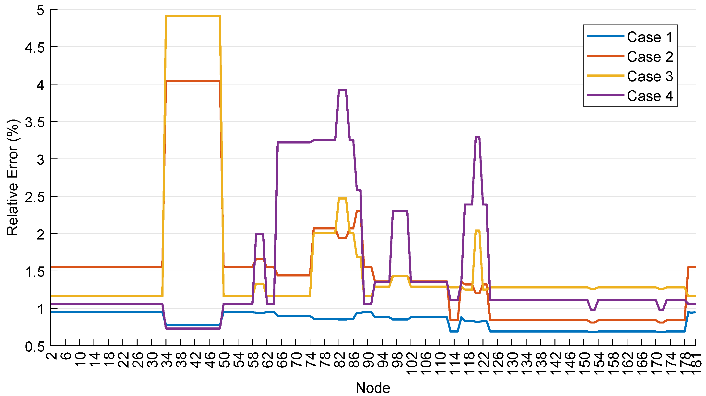
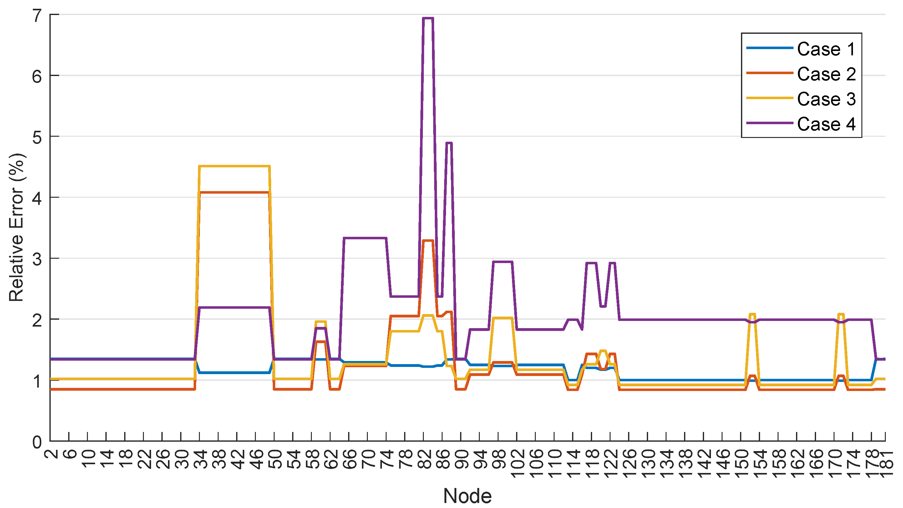
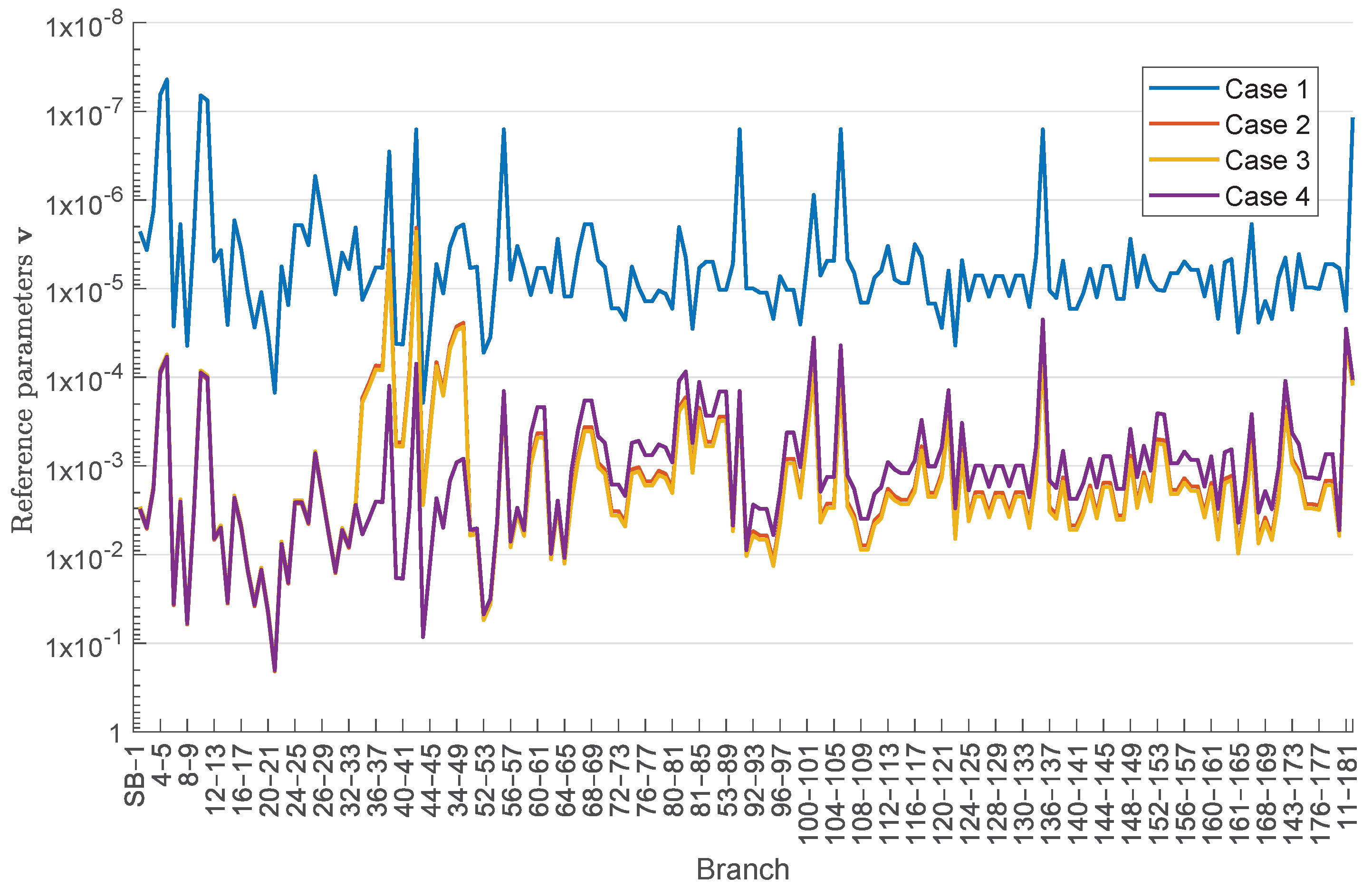
Figure 2 and Figure 3 show the relative error for the load point failure rates and outage times, respectively. Notice that a large amount of the load point indices do not converge with 1% relative error. In cases 2 and 3, the relative errors of load point indices are significantly greater than those acquired in case 1. Figure 2 shows that the relative errors between node 35 and 48 obtained in cases 2 and 3 are approximately 5 times greater than in case 1. Indeed, the design of the CE optimization function, which relies on the systemic indices to optimize the reference parameters, results in a prioritization of the nodes that contribute more to the systemic index. Since the nodes between node 35 and 48 have only nine customers, the optimized parameters for their laterals (branch 35 to 48) are not significantly different from their original counterparts, as shown in the inverse log graphic in Figure 4. The pattern in the relative errors in Figure 2 are similar for cases 2 and 3. Nevertheless, the same conclusion cannot be extended for the results in Figure 3. The outage time relative error for load points between nodes 35 and 48 increases in cases 2 and 3. The same is observed between nodes 76 and 88, but with relative error greater in case 2 than in case 3.
In case 4, the SAIDI index estimate does not reach the relative error β used in other cases, achieving a value of 1.41%. In Figure 4, it is possible to observe that the reference parameters of nodes 35 to 48 are greater in comparison with all other optimized cases for case 4. However, the reference parameters assume reduced values for components that do not affect straightforwardly, in the reliability sense, node 40, in comparison to cases 2 and 3. These reference parameters are impacted mostly by selecting SAIFI as one of the objective functions. The choice of λ 40 as one of the objective functions affects the relative errors of all other load point indices, as shown in Figure 2 and Figure 3, where high relative errors can be found for components which do not affect straightforwardly node 40 in its reliability.

5. Discussion and Final Remarks

This paper proposes a multi-objective CE approach for power distribution system reliability evaluation, considering systemic and load point indices. As main contribution, a mathematical deduction of an analytical solution for the multi-objective CE optimization problem is devised, taking into account the standard hypotheses utilized in distribution system reliability assessments. Using a single-objective function, one can optimize only the convergence of a single index, whereas other relevant aspects of the system quantified by other indices are neglected. When a multi-objective function is applied, then multiple indices can be prioritized in the variance reduction and a faster simulation can be achieved.
The key requirement for the applicability of our method is the ability to analytically compute the conditional indices (e.g., E [ H ( X ) | X j = 1 ] ) used as inputs. While all deductions in the paper are valid, their practical application might be compromised if non-standard reliability evaluation assumptions are used [14,15], as the computation of these input indices would no longer be straightforward. Nonetheless, by using the standard reliability assumptions, the proposed method provides an interesting alternative to iterative CE approaches for a wide range of practical distribution systems.
Future works will address the application of different methods to solve the multi-objective CE optimization problem as well as a detailed analysis of the advantages and drawbacks of utilizing the CE method. This includes investigating the trade-off between reducing the number of simulated years and the increased computational burden from a high number of sampled failures per year. A concern to be studied is the possibility that an overly high optimized failure rate could increase the total simulation processing time, even as it successfully decreases the required number of simulated years.

Author Contributions

Conceptualization, L.F.V. and D.I.; methodology, L.F.V. and D.I.; software, L.F.V.; validation, L.F.V., L.M.C. and D.I.; formal analysis, L.F.V. and D.I.; investigation, L.F.V., B.S.B. and D.I.; resources, D.I.; data curation, L.M.C.; writing—original draft preparation, L.F.V. and D.I.; writing—review and editing, L.F.V., B.S.B., E.P.d.S., L.M.C. and D.I.; visualization, L.F.V.; supervision, L.M.C. and D.I.; project administration, D.I.; funding acquisition, D.I. All authors have read and agreed to the published version of the manuscript.

Funding

This work was developed in Project “New Elements of Grid Automation, with Advanced Function of Distributed Intelligence” with EDP Brasil, under the framework of the Research and Development (R&D) Program regulated by Brazilian Electricity Regulatory Agency (ANEEL), code PD-00380-0027/2018. This research has also been funded by Brazilian Coordination for the Improvement of Higher Education Personnel (CAPES), National Council for Scientific and Technological Development (CNPq), and INESC P&D Brasil.

Data Availability Statement

The datasets presented in this article are not readily available because the authors do not have permission to share data. Requests to access the datasets should be directed to diego.issicaba@ufsc.br.

Acknowledgments

The authors would like to acknowledge CAPES and CNPq for supporting this research activity.

Conflicts of Interest

Author Lucas Fritzen Venturini was employed by the CELESC Distribuição S.A. The remaining authors declare that the research was conducted in the absence of any commercial or financial relationships that could be construed as a potential conflict of interest.

References

  1. Rubinstein, R.Y.; Kroese, D.P. The Cross-Entropy Method: A Unified Approach to Combinatorial Optimization, Monte-Carlo Simulation and Machine Learning (Information Science and Statistics); Springer: New York, NY, USA, 2004. [Google Scholar]
  2. Rubinstein, R.Y.; Kroese, D.P. Simulation and the Monte Carlo Method, 3rd ed.; Wiley Publishing: Hoboken, NJ, USA, 2016. [Google Scholar]
  3. Leite da Silva, A.M.; Fernandez, R.A.G.; Singh, C. Generating Capacity Reliability Evaluation Based on Monte Carlo Simulation and Cross-Entropy Methods. IEEE Trans. Power Syst. 2010, 25, 129–137. [Google Scholar] [CrossRef]
  4. Gonzalez-Fernandez, R.A.; Leite da Silva, A.M. Reliability Assessment of Time-Dependent Systems via Sequential Cross-Entropy Monte Carlo Simulation. IEEE Trans. Power Syst. 2011, 26, 2381–2389. [Google Scholar] [CrossRef]
  5. González-Fernández, R.A.; Leite da Silva, A.M.; Resende, L.C.; Schilling, M.T. Composite Systems Reliability Evaluation Based on Monte Carlo Simulation and Cross-Entropy Methods. IEEE Trans. Power Syst. 2013, 28, 4598–4606. [Google Scholar] [CrossRef]
  6. Carvalho, L.M.; González-Fernández, R.A.; Leite da Silva, A.M.; da Rosa, M.A.; Miranda, V. Simplified Cross-Entropy Based Approach for Generating Capacity Reliability Assessment. IEEE Trans. Power Syst. 2013, 28, 1609–1616. [Google Scholar] [CrossRef]
  7. Leite da Silva, A.M.; Costa Castro, J.F.; González-Fernández, R.A. Spinning Reserve Assessment Under Transmission Constraints Based on Cross-Entropy Method. IEEE Trans. Power Syst. 2016, 31, 1624–1632. [Google Scholar] [CrossRef]
  8. Zhao, Y.; Tang, Y.; Li, W.; Yu, J. Composite Power System Reliability Evaluation Based on Enhanced Sequential Cross-Entropy Monte Carlo Simulation. IEEE Trans. Power Syst. 2019, 34, 3891–3901. [Google Scholar] [CrossRef]
  9. Urgun, D.; Singh, C.; Vittal, V. Importance Sampling Using Multilabel Radial Basis Classification for Composite Power System Reliability Evaluation. IEEE Syst. J. 2020, 14, 2791–2800. [Google Scholar] [CrossRef]
  10. Urgun, D.; Singh, C. Composite Power System Reliability Evaluation Using Importance Sampling and Convolutional Neural Networks. In Proceedings of the 2019 20th International Conference on Intelligent System Application to Power Systems (ISAP), New Delhi, India, 10–14 December 2019; pp. 1–6. [Google Scholar] [CrossRef]
  11. Cordeiro Vieira, P.C.; Da Rosa, M.A.; Leite Da Silva, A.M. Long-Term Operating Reserve Assessment of Power Systems with Variable Renewable Generation via Cross-Entropy Method. In Proceedings of the 2022 17th International Conference on Probabilistic Methods Applied to Power Systems (PMAPS), Manchester, UK, 12–15 June 2022; pp. 1–6. [Google Scholar] [CrossRef]
  12. Manso, B.A.S.; Leite da Silva, A.M.; Milhorance, A.; Assis, F.A. Composite reliability assessment of systems with grid-edge renewable resources via quasi-sequential Monte Carlo and cross-entropy techniques. IET Gener. Transm. Distrib. 2024, 18, 326–336. [Google Scholar] [CrossRef]
  13. Hanna, R.; Disfani, V.R.; Kleissl, J. Reliability Evaluation for Microgrids Using Cross-Entropy Monte Carlo Simulation. In Proceedings of the 2018 IEEE International Conference on Probabilistic Methods Applied to Power Systems (PMAPS), Boise, ID, USA, 24–28 June 2018; pp. 1–6. [Google Scholar] [CrossRef]
  14. Billinton, R.; Allan, R.N. Reliability Evaluation of Power Systems; Springer: Boston, MA, USA, 1996. [Google Scholar] [CrossRef]
  15. Brown, R.E. Electric Power Distribution Reliability; Power Engineering (Willis); CRC Press: Boca Raton, FL, USA, 2008. [Google Scholar]
  16. Amarasinghe, P.; Abeygunawardane, S.; Singh, C. Reliability evaluation of solar integrated power distribution systems using an Evolutionary Swarm Algorithm. Eng. Appl. Artif. Intell. 2025, 149, 110464. [Google Scholar] [CrossRef]
  17. Soni, Y.P.; Fernandez, E. A novel approach for techno-economic reliability oriented planning and assessment of droop-control technique for DG allocation in islanded power distribution systems. Electr. Power Syst. Res. 2024, 234, 110601. [Google Scholar] [CrossRef]
  18. Kumar, B.; Saw, B.K.; Bohre, A.K. Optimal Distribution Network Reconfiguration to Improve the System Performances using PSO with Multiple-Objectives. In Proceedings of the 2020 International Conference on Computational Intelligence for Smart Power System and Sustainable Energy (CISPSSE), Keonjhar, India, 29–31 July 2020; pp. 1–6. [Google Scholar] [CrossRef]
  19. Pattabiraman, S.; Sampath, K.; Kannan, M.; Girish, G.R.; Narayanan, K. Reliability Improvement in Radial Distribution System through Reconfiguration. In Proceedings of the 2019 IEEE Innovative Smart Grid Technologies-Asia (ISGT Asia), Chengdu, China, 21–24 May 2019; pp. 1963–1967. [Google Scholar] [CrossRef]
  20. Senthilkumar, S.; Balachander, K.; Mohamed Mansoor, V. A hybrid technique for impact of hybrid renewable energy systems on reliability of distribution power system. Energy 2024, 306, 132383. [Google Scholar] [CrossRef]
  21. dos Reis, T.P.; Raizer, A. Multi-objective optimization of reliability and cost efficiency in lightning protection for overhead distribution systems. Electr. Power Syst. Res. 2025, 248, 111904. [Google Scholar] [CrossRef]
  22. Ebrahimi, M.; Rastegar, M. Optimal planning of fault interrupter and load break switches in power distribution systems: A linear power flow-constrained multi-objective optimization. Reliab. Eng. Syst. Saf. 2025, 264, 111457. [Google Scholar] [CrossRef]
  23. Lu, J.; Yan, X.; Jia, J.; Shao, C.; Han, L.; Cai, W. Bi-level planning of rotary power flow controllers and energy storage systems for economy and carrying capacity improvement in the distribution network. Int. J. Electr. Power Energy Syst. 2025, 171, 110917. [Google Scholar] [CrossRef]
  24. de Assis, L.S.; Epifanio, G.P.; Usberti, F.L.; González, J.F.V.; Cavellucci, C. Evolutionary algorithms for switch allocation in power distribution networks with distributed generation. Electr. Power Syst. Res. 2025, 249, 112013. [Google Scholar] [CrossRef]
  25. Bekker, J.; Aldrich, C. The cross-entropy method in multi-objective optimisation: An assessment. Eur. J. Oper. Res. 2011, 211, 112–121. [Google Scholar] [CrossRef]
  26. Botev, Z.I.; Kroese, D.P.; Rubinstein, R.Y.; L’Ecuyer, P. Chapter 3-The Cross-Entropy Method for Optimization. In Handbook of Statistics; Rao, C., Govindaraju, V., Eds.; Elsevier: Amsterdam, The Netherlands, 2013; Volume 31, pp. 35–59. [Google Scholar] [CrossRef]
  27. Lobato, F.S.; Steffen, V.S., Jr. Multi-Objective Optimization Problems: Concepts and Self-Adaptive Parameters with Mathematical and Engineering Applications; Springer International Publishing: Berlin/Heidelberg, Germany, 2007. [Google Scholar]
  28. Baracy, Y.L.; Venturini, L.F.; Branco, N.O.; Issicaba, D.; Grilo, A.P. Recloser placement optimization using the cross-entropy method and reassessment of Monte Carlo sampled states. Electr. Power Syst. Res. 2020, 189, 106653. [Google Scholar] [CrossRef]
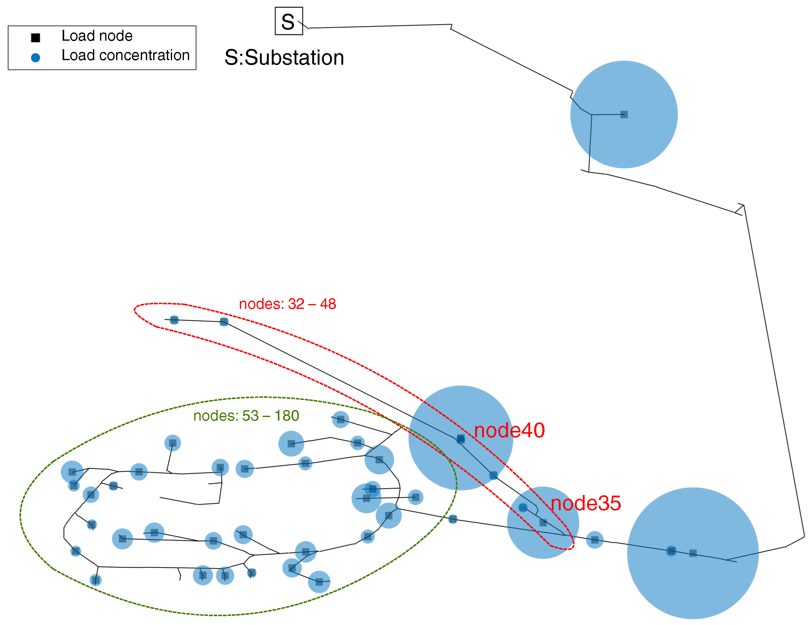
Figure 1. Brazilian real feeder under analysis [28].
Energies 18 06421 g001
Figure 2. Relative errors for load point failure rates in all simulation cases.
Energies 18 06421 g002
Figure 3. Relative errors for load point outage times in all simulation cases.
Energies 18 06421 g003
Figure 4. Reference parameters v for all simulation cases.
Energies 18 06421 g004
Table 1. Results for the simulated cases.
CasesSAIFI
(occ/yr)
SAIDI
(h/yr)
ENS
(kWh/yr)
Number of
Sampled Years
Number of
Failures
11.58397.791914,777983533,310
21.59397.614614,6071222,525
31.56647.593515,038916,553
41.56967.671714,564711,291
Disclaimer/Publisher’s Note: The statements, opinions and data contained in all publications are solely those of the individual author(s) and contributor(s) and not of MDPI and/or the editor(s). MDPI and/or the editor(s) disclaim responsibility for any injury to people or property resulting from any ideas, methods, instructions or products referred to in the content.