Abstract
Conventionally, tomography is an inspection technique in which tomographic images are intended for human perception and interpretation. In this work, we shift this paradigm by transforming tomography into an autonomous estimator of industrial reactor states, enabling fully automated process control. Alcoholic fermentation was employed as an example of a controlled process in the current study. The work presents an original concept utilizing transfer learning in conjunction with a ResNet-type artificial neural network, which converts electrical measurements into a sequence of values correlated with the conductivity of pixels constituting the cross-section of the examined biochemical reactor. The conductivity vector is transformed into a parameter determining substrate concentration, enabling dynamic process regulation in response to signals generated from EIT (Electrical Impedance Tomography). Within the scope of the described research, calibration of the conductivity vector against substrate concentrations was performed, and a Matlab/Simulink-based dynamic Monod kinetics model was developed. The obtained results demonstrate high accuracy in substrate concentration estimation relative to reference values throughout a forty-six-hour process. The same signals enable energy-efficient process control, in which cooling and mixing intensity are regulated according to energy prices and renewable energy availability. This strategy may possess particular application in facilities where fermentation installations are co-located with bioenergy production units.
1. Introduction
1.1. Background and Related Work
Modern process plants in the chemical, food, pharmaceutical and water–wastewater sectors are moving from reactive control to proactive strategies under Quality by Design and Process Analytical Technology (PAT) frameworks [1,2]. The central challenge in continuous operations is to recover reliable, non-invasive and disturbance-resistant information about the internal state of equipment under flowing streams, strong couplings, and hard operating constraints. Point sensors such as pH, conductivity, temperature and flow are valuable but inherently local, which is often insufficient for precise model-based control in the presence of heterogeneous fields [3,4]. Spectrophotometry (UV–Vis) is widely used to quantify key analytes via the Beer–Lambert relationship between absorbance, concentration, and optical path length. In practice, measurements are often performed off-line on extracted samples, although in-line fiber-optic implementations exist within PAT deployments [5]. By contrast, tomography provides spatially resolved information suitable for machine-readable state estimation at high refresh rates.
Process tomography addresses this gap by providing cross-sectional images of physical quantities that correlate with the composition and structure of the medium. Several modalities are used in practice, including electrical impedance tomography (EIT) [6,7], electrical capacitance tomography (ECT) [7,8], ultrasound tomography (UST) [9,10], nuclear magnetic resonance (NMR) or magnetic resonance imaging (MRI) [11], and optical coherence tomography (OCT) [12,13]. Among these, EIT stands out for its bioprocess safety, comparatively low hardware cost, high sampling rates and ease of integration with production lines. Its inverse problem is ill-posed and sensitive to contact artifacts, yet recent methods in image reconstruction and physics-aware data fusion have markedly reduced these limitations and improved readiness for online deployment [14,15,16]. In bioreactors, practical confounders such as electrode polarization and fouling, temperature and ionic strength drifts, and gas holdup from CO2 must be addressed through design and compensation. Practical demonstrations in low conductivity systems, e.g., combining electrical impedance spectroscopy with 2D electrical resistance tomography to monitor antisolvent crystallization, further illustrate the potential of impedance-based imaging for industrial monitoring [17].
Beyond diagnostic use, several studies show that tomographic measurements can support control decisions in particulate processes. In control-oriented frameworks, ECT images or derived features are used to regulate multiphase flows and fluidized beds, indicating practical pathways toward closed-loop operation in continuous settings [18]. At the same time, high-speed ECT systems have been demonstrated for online monitoring of pneumatic conveying with acquisition rates in the hundreds of frames per second, meeting the timing requirements of industrial supervision and control [19].
Biotechnological processes, including alcoholic fermentation, are a natural application for EIT. Bioethanol production is carried out in batch, semi continuous and continuous modes. Decision variables include dilution factor , nutrient doses, temperature, early aeration, and cooling and mixing schedules. Substrate, biomass, and product concentrations are strongly correlated with solution conductivity and its distribution. Conductivity maps can therefore power soft sensors for hidden state estimation and subsequently for monitoring and predictive control. In recent years, machine learning based soft sensor solutions for fermentation have been presented, including variants designed and maintained according to Machine Learning Operations (MLOps) practices [20], as well as in-line implementations using Raman and Near Infrared Spectroscopy (NIR) spectroscopy [21], and electronic noses [22]. A similar trend is demonstrated by work combining impedance sensors with data models for ethanol and biomass monitoring [23].
Progress over the last few years shows that combining EIT with deep learning image reconstruction, and with non-structured kinetic models such as Monod relations with inhibitions, improves the stability and repeatability of process state estimation [24,25]. The resulting processing chain from EIT measurements through image reconstruction and feature extraction to a soft sensor, followed by an observer and controller, enables not only tight feedback but also supervisory control. In supervisory layers, schedules of energy-intensive auxiliaries such as cooling, recirculation and pumps can be coordinated with technological constraints and energy price or availability signals, which is increasingly relevant under high shares of renewables [14,15]. Related industrial studies also explore energy recovery options in auxiliary systems, e.g., compressed-air engines, underscoring the broader context for energy-aware operation [26]. These observations define a pathway in which tomographic sensing advances from diagnostics to an active component of control architectures for continuous bioprocessing. EIT provides spatially resolved fields that can be converted into stable numerical features and linked to process kinetics with latency compatible with real-time decision making. In this systems view, the primary objective is not image appearance but the stability, informativeness, and timeliness of features that support observers, feedback regulation, and energy-aware supervision under industrial constraints.
1.2. Motivation, Novelty and Paper Structure
The increasing penetration of renewable energy sources into power systems necessitates advanced monitoring and control strategies to ensure stability, efficiency, and resilience. Industrial process control faces similar challenges, as complex, nonlinear, and spatially distributed processes must be monitored and regulated in real time to meet quality, safety, and energy-efficiency requirements. In this context, process tomography has emerged as a promising tool for non-invasive visualization of internal states in biochemical tank reactors and pipelines. Electrical Impedance Tomography (EIT) is particularly attractive because of its low-cost instrumentation, high sampling rates, and ability to operate under industrial conditions without interrupting production.
While EIT has been extensively studied for monitoring and diagnostic purposes, its application to automatic, unattended process control remains largely unexplored. Existing literature has primarily focused on producing tomograms interpretable by human operators, emphasizing visual clarity and inclusion detectability. However, when EIT is used as part of a closed-loop control system, the human operator is no longer the primary recipient of the reconstructed images. Instead, the outputs must serve as numerical features that enable automated decision-making. In this paradigm, the visual quality of the reconstruction is secondary, as the controller consumes vectors of features or scalar indicators derived from tomograms to regulate the process in real time. This conceptual shift—from human-centered visualization to machine-readable state estimation—represents the key novelty of this work.
The primary objective of this research is to transform Electrical Impedance Tomography (EIT) from a diagnostic imaging tool into an autonomous process control sensor for biochemical systems, specifically addressing the gap between traditional human-interpreted tomographic visualization and automated industrial process control. This study aims to develop and validate an integrated framework that converts EIT measurements directly into machine-readable state vectors, eliminating the need for human interpretation of tomographic images in closed-loop control applications. The specific goals include (1) establishing a paradigm shift from visual tomogram interpretation to numerical feature extraction for automated decision-making, (2) integrating real-time EIT measurements with Monod kinetics modeling to enable accurate state estimation of fermentation processes, and (3) demonstrating energy-efficient process control by coordinating tomography-informed decisions with external energy constraints such as renewable energy availability and demand-response signals.
The proposed framework integrates EIT-based state reconstruction with machine learning models for feature extraction and prediction, followed by supervisory control algorithms that can adjust process variables such as dilution rate, temperature, and mixing schedules. This approach allows the coordination of process dynamics with external energy constraints, including demand-response signals and renewable energy availability, which is crucial for sustainable operation in modern distributed energy systems.
The remainder of the paper is organized as follows. Section 2 describes the fermentation process selected as a representative industrial case study and details the experimental setup and the EIT data acquisition system. The machine learning-based reconstruction and feature extraction pipeline, as well as the kinetic modeling approach, are also introduced. Section 3 presents simulation results demonstrating the closed-loop behavior of the system under repeated batch fermentation cycles. Section 4 discusses the implications of using EIT for process control, its advantages and limitations, and the potential for integration with energy-aware scheduling. Finally, Section 5 summarizes the main contributions and outlines future research directions, including extension to other industrial processes and coupling with advanced energy management frameworks.
2. Materials and Methods
2.1. Description of the Alcoholic Fermentation Process
Fermentation is observed in natural environments and is widely applied across numerous production domains. Depending on the specific pathway, various gases are released. It is defined as an anaerobic mode of respiration performed by many bacteria and certain fungi. During fermentation, the respiratory substrate is decomposed and transformed, with one product undergoing oxidation and another reduction. Energy is generated and stored as ATP (adenosine 5′-triphosphate). Based on the principal end product, lactic, butyric, acetic, alcoholic, and methanogenic fermentation are distinguished [27]. Alcoholic fermentation is considered here as the target process for sensing and control. It is defined as the anaerobic conversion of carbohydrates, predominantly by Saccharomyces cerevisiae, that yields ethanol and carbon dioxide. The process is widely used in the distilling, brewing, and wine industries. Its biological basis is the ability of yeast to hydrolyze and process simple sugars in the presence of appropriate enzymes.
The choice of alcoholic fermentation is motivated by practical considerations that support stable operation and reproducible experimentation. The course of alcoholic fermentation under typical conditions is predictable and relatively insensitive to moderate temperature variation, which facilitates controlled trials. From a monitoring perspective, the primary observable is the spatiotemporal evolution of bulk electrical conductivity inside the fermenter. Conductivity depends on the concentration of ions dissolved in the aqueous phase and on the accumulation of fermentation products. In alcoholic fermentation, fermentable sugars are initially present in solution and ethanol is a principal product with a characteristic electrical signature, so the conductivity of the medium changes in a gradual and trackable manner as sugars are converted to ethanol and carbon dioxide.
At the biochemical level, fermentable sugars such as glucose, fructose, and sucrose enter glycolysis to form pyruvate. Pyruvate is then decarboxylated to acetaldehyde and reduced to ethanol, and during this reduction, the oxidized form of nicotinamide adenine dinucleotide is regenerated, which maintains redox balance and allows glycolysis to continue under oxygen limitation [28]. A canonical overall stoichiometry on glucose is (1)
which summarizes the conversion to ethanol and carbon dioxide with substrate-level phosphorylation. Saccharomyces cerevisiae is preferred in industrial practice because it combines rapid uptake and metabolism of sugars with tolerance to osmotic stress and elevated ethanol concentrations, supported by membrane remodeling and other stress response mechanisms [29,30]. The organism grows best in mildly acidic media and requires yeast assimilable nitrogen and micronutrients for enzyme synthesis and balanced growth, and the availability of these nutrients modulates both the fermentation rate and the formation of secondary metabolites [31].
The temporal evolution of the process begins with a short adaptation phase, after which active fermentation proceeds with rapid sugar depletion, biomass growth, and increasing formation of ethanol and carbon dioxide. As residual sugars decline and ethanol accumulates, the culture enters a decelerating phase that culminates in completion when sugars are exhausted or when inhibitory thresholds are reached. Product inhibition by ethanol, substrate inhibition at very high initial sugar concentrations, and nutrient limitations are the principal kinetic constraints. Operating conditions are typically mesophilic and mildly acidic, with agitation adjusted to maintain homogeneity and effective mass and heat transfer while avoiding excessive shear. Oxygen is minimized after the early adaptation period to favor fermentative metabolism, although brief controlled oxygen exposure at the start can support sterol and unsaturated fatty acid synthesis that stabilizes cell membranes. Alongside ethanol and carbon dioxide, minor compounds such as higher alcohols, organic acids, and esters are formed, and their concentrations depend on strain genetics, substrate composition, temperature, and nutrient status. Endpoint determination is based on the depletion of fermentable sugars to target levels and on the approach of carbon dioxide evolution and ethanol formation rates to quasi-steady values, subject to quality and safety specifications [32].
The conductivity → concentration mapping used in this research is an empirical, linear calibration fitted to alcoholic fermentation under our operating window, with a proportionality coefficient of 0.99 kg·m−3 per conductivity unit and an offset of −0.85 kg·m−3. This calibration is expected to transfer across batches with similar media, temperature, and ionic strength, but we treat it as site- and recipe-specific: different substrate compositions, yeast strains, or temperature profiles alter conductivity–chemistry coupling and typically require re-fitting the coefficients using a small set of paired EIT and reference measurements. Within a given facility, linearity has proven adequate over the relevant concentration range. If departures from linearity appear (e.g., due to high ethanol or strong ionic changes), we will adopt piecewise-linear or multivariable calibrations that incorporate temperature compensation and auxiliary probes while preserving the same estimation and control architecture.
2.2. Experimental Setup
The entire experimental stand, including the measurement vessel, the wireless sensor modules, and the electrical impedance tomography device, was manufactured by Netrix S.A. (Lublin, Poland). The experimental stand comprised a measurement vessel, a stirring system, and an integrated suite of sensors. The vessel was instrumented for electrical impedance tomography and operated as a bench-scale fermenter. Two circumferential rings of electrodes were mounted on the vessel wall in fixed positions in order to define a reproducible tomographic boundary, with the lower ring carrying electrodes one through sixteen and the upper ring carrying electrodes seventeen through thirty-two. Mixing was provided by a magnetic stirrer placed beneath the vessel, which avoided mechanical penetrations and mitigated flow-related artefacts in the vicinity of the electrode planes (Figure 1). Process pH was measured in the central region of the vessel using a laboratory pH meter (Figure 1b). Air temperature, relative humidity, and barometric pressure were monitored continuously during each run. Process temperature was measured at three locations to capture vertical gradients and boundary effects. One probe was located below the vessel, one above the vessel, and one within the liquid column between the two electrode rings.
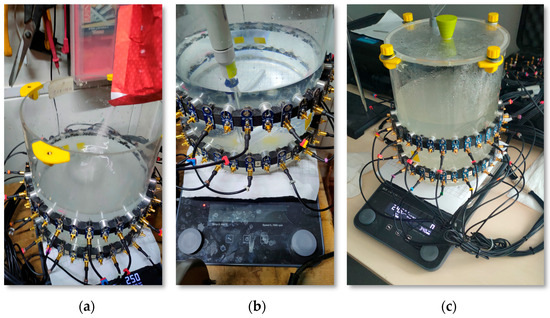
Figure 1.
Tank reactor with EIT electrodes and the magnetic stirrer: (a) adding substrate (sugar) to the vessel; (b) pH measurement; (c) controlled fermentation process in a closed vessel.
The principal process variable of interest was the electrical conductivity of the liquid phase. Conductivity depends on the concentration of dissolved ions and on the presence and evolution of fermentation products. During alcoholic fermentation, the progressive conversion of dissolved sugars to ethanol and carbon dioxide results in a gradual and measurable change in bulk conductivity, which provides an informative signature for subsequent analysis. The preparation of the medium followed a standard protocol. Three and a half liters of water were introduced into the vessel and one kilogram of sugar was added and mixed until fully dissolved. After complete dissolution, 23.37 g of dry distiller’s yeast were added as inoculum. The vessel equipped with the electrode array was positioned on the magnetic stirrer and mixing was initiated. The preparations for the sugar solution and inoculation are documented in Figure 1a.
To perform measurements on a real physical model, a prototype EIT device designed and manufactured in the Netrix SA laboratory was used (Figure 2).
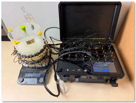
Figure 2.
Measurement setup: prototype EIT device connected to the physical tank reactor model.
Data acquisition and sequencing were coordinated by the STMicroelectronics STM32F746G DISCO Discovery board (Agrate Brianza, Italy). The board is built around the STM32F746NGH6 microcontroller with an ARM Cortex M7 core clocked at 216 MHz. It provides 1 MB of embedded flash memory and 340 KB of static random access memory. Local human–machine interaction is supported by a color TFT LCD with a diagonal of 4.3 in, a resolution of 480 × 272 pixels, and a 16-bit color palette, together with a capacitive touch layer. A wired network interface compliant with IEEE 802.3-2002 [33] is available through an RJ-45 connector and operates at 10/100 Mb/s. The direct current section of the measurement and multiplexing board supplies regulated rails at 5 V and 3.3 V for the sensing subsystems.
Excitation and measurement paths are routed through a switching matrix composed of 32 CMOS analog keys of the Vishay DG413 family, driven by 2 Texas Instruments CD74HC154M 16-channel decoders (Dallas, TX, USA). The matrix is arranged as an H bridge so that all non-active lines are referenced to ground. Excitation paths and measurement paths are switched by separate keys in order to limit crosstalk and leakage. Power for the control electronics is provided at 5 V, while peripheral circuits are supplied from the 5 V and 3.3 V rails as required.
The tomograph device was connected to the vessel outfitted with the 32-electrode array. Two rings of sixteen electrodes provided 32 channels for current injection and potential measurement. A single 16-electrode ring configuration was used, despite the availability of two rings, for several key reasons. Primarily, this choice enforces a two-dimensional (2D) cross-sectional assumption, which was essential for maintaining a fixed and repeatable boundary for training the ResNet50 reconstructor. This approach also avoids confounding vertical effects that would otherwise necessitate a more complex 3D or multi-ring forward model and complete network retraining.
Operationally, the single-ring configuration offered significant practical advantages, including simplified calibration, reduced data acquisition and processing complexity, and improved run-to-run comparability under controlled stirring. We acknowledge that this configuration results in a lower angular sampling density compared to a 32-electrode setup, which inherently limits fine-scale spatial discrimination. However, this trade-off was deemed acceptable as the primary objective was the robust recovery of machine-readable state variables (e.g., average substrate concentration) rather than high-resolution imaging. For this application, which relies on spatially averaged data, the 16-electrode ring provided the necessary stability and accuracy. We have clarified this rationale and its impact on spatial resolution in the manuscript and note that extending the system to dual-ring or full 3D acquisition is a planned direction for future work.
The instrument operated at a frequency of one kilohertz and applied an excitation current of two thousand microamperes to each driven electrode. The fixed geometry of the electrode rings and the repeatable stirring conditions ensured comparability across runs and supported time-resolved analysis of conductivity changes within the liquid. Reconstruction of conductivity fields from EIT measurements is performed with a convolutional ResNet50. Features extracted from the reconstructed images are subsequently supplied to the kinetic model described later (Section 2.3), which is used for state estimation and short-term prediction of the fermentation process.
To enhance clarity, a methodological workflow diagram (Figure 3) summarizes the proposed pipeline, illustrating the sequential transformation from raw EIT measurements through neural network-based reconstruction and kinetic modeling to closed-loop supervisory control.
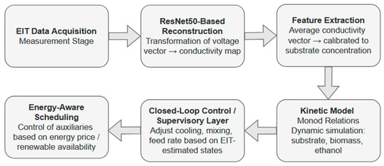
Figure 3.
Methodological workflow of the proposed EIT-based monitoring and control framework.
The choice of ResNet50 was motivated by its stable reconstruction performance across a wide range of geometries and bulk conductivities, yielding reliable estimates of key states (e.g., substrate concentration). The neural network used had an input vector of 96 voltage measurements and an output vector of 2502 values correlated with the conductivity of the finite elements of the finite element mesh (FEM): . The detailed method for obtaining the EIT simulation measurements necessary to train the neural network is explained in the publication [7]. The deep neural network model comprised 175 layers interconnected through 190 connections and included 214 sets of learnable parameters as well as 106 stateful parameters. The network accepted input through a designated input port and produced outputs via a final fully connected layer mapping to 2502 outputs. Training was conducted using the Adam optimizer over a maximum of 500 epochs, with mini-batches of size 64. In each epoch, the training dataset was shuffled, and variable-length sequences were accommodated by grouping inputs into batches of the maximal sequence length encountered. Validation was performed on a separate held-out dataset at intervals of every 100 iterations, and early stopping was applied if validation performance did not improve over 200 consecutive checks. The root-mean-square error (RMSE) metric was used to monitor performance, and training progress was visualized dynamically. Computations were executed on the available hardware platform, adapting to Graphics Processing Unit (GPU) resources. During training, gradients were backpropagated through the entire network (including recurrence or temporal dependencies where present), and parameter updates followed the Adam update rules. The early stopping mechanism prevented overfitting by halting training when further refinements on the validation set stalled. All layers, residual connections, and internal transformations (e.g., convolutional, normalization, and activation) were optimized simultaneously under this regimen. Figure 4 shows the training performance of the ResNET50 through RMSE. Convergence of the error lines for the training and validation sets indicates the absence of overfitting. The green triangle indicates the iteration for which the model generated the smallest RMSE error. Training was automatically stopped by a specified early stopping condition, which included 200 consecutive epochs without decreasing the loss function value. The regular, hyperbolic shape of the graph and the lack of fluctuations indicate the absence of overfitting.
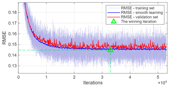
Figure 4.
Training performance of .
2.3. Simulation Environment
The simulation model shown in Figure 5 implements a dynamic closed feedback loop in which the course of alcoholic fermentation is simulated using information about the spatial distribution of electrical conductivity inside the reactor. The workflow begins by loading a conductivity map from a database of tomographic reconstructions. The map represents local conductivity values on a finite element mesh of 2502 cells/pixels and serves as an indirect indicator of the distribution of dissolved species in the broth. The getSigma block retrieves the current conductivity vector from the base workspace and provides it to the Simulink model. It ensures a fixed output size and allows the simulation to use the most recent conductivity data updated by other blocks, such as trigger_plot_sfun. The conductivityToConcentration block converts the conductivity distribution into a state vector describing the process conditions. It applies a linear calibration to estimate substrate concentration, then sums the results to obtain its overall value in the reactor. Biomass and ethanol concentrations are set to constant reference values. The resulting vector is used as input for Fb_function and the Integrator, linking tomographic data with the dynamic fermentation model and enabling EIT-based simulation. The trigger_plot_sfun block monitors the process state and triggers updates of the conductivity distribution used for EIT reconstruction. At the start of the simulation, it generates an initial conductivity field and activates the reset signal. During simulation, it checks the substrate concentration and, when it falls below a threshold, loads a new conductivity vector, updates the FEM image, and refreshes the visualization window. A cooldown mechanism prevents repeated triggering until the concentration rises again, ensuring controlled and synchronized updates of the model state. The Scope block in Simulink is used to visualize signals in real time during simulation.
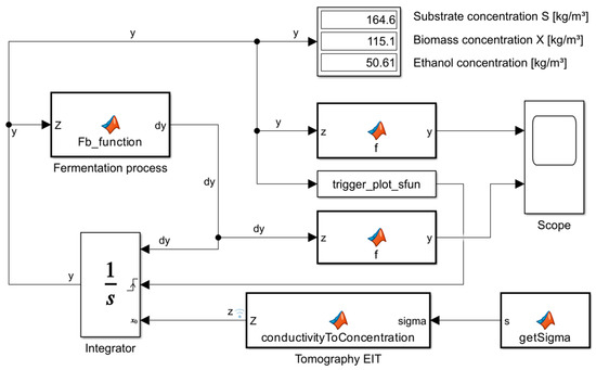
Figure 5.
Schematic diagram of the simulation model of the alcoholic fermentation process.
The conductivity field is converted to an average substrate concentration through a linear calibration fitted to prior experiments. The calibration uses a proportionality coefficient of per unit of conductivity and an offset of . In the baseline configuration, the concentrations of biomass and ethanol are fixed at and . These constants stabilize the numerical scheme and isolate the dynamics of the substrate. They can be released in later variants to represent their time evolution.
The three-component concentration vector obtained from the calibrated conductivity is forwarded to a kinetic core based on Monod relations [34]. The Monod dependence used in the kinetic core is (2)
where is the maximal specific growth rate scaled to a 46 h simulation window and is the substrate saturation constant. Stoichiometric yields that link substrate consumption to biomass formation and ethanol production are 0.1 for biomass on substrate and 0.5 for ethanol on substrate [34]. The model computes instantaneous rates from these parameters and advances the state in time by numerical integration. The Integrator block performs continuous-time integration of the input signal, updating the process state over simulation time. It is configured with an external reset that reinitializes the state whenever a rising edge signal is detected, allowing the system to restart from new initial conditions when required.
Based on the computed specific growth rate, the reaction rates are obtained as biomass formation , substrate consumption , and ethanol formation . The output of the kinetic block is the three-dimensional vector of time derivatives corresponding to changes in concentrations: substrate loss , biomass growth and ethanol production . This vector is then passed to the integrator block in the Simulink model, which allows for a continuous evolution of the system state over time.
An event mechanism introduces realistic variability in internal conditions. If the simulated substrate concentration falls below the model draws a new conductivity map from the reconstruction database and inserts it into the next simulation step. This refresh emulates the evolving physical and chemical environment inside the fermenter and prevents the trajectory from locking into a single spatial pattern. The update is protected by cooldown logic so that two updates cannot occur in direct succession. This avoids excessive perturbations and maintains numerical stability.
The MATLAB Simulink R2025a interface is configured to stream conductivity maps during execution. A block retrieves the current map from the MATLAB base workspace and enforces a fixed vector length equal to the mesh size. A companion block converts the conductivity to concentrations using the specified linear calibration and outputs a three-component state vector. A supervisor block monitors the current state and issues a trigger when the threshold condition is met. The visualization routine reuses an existing plot window and redraws the finite element field each time a new map is injected. This provides a continuous view of the evolving distribution throughout the run.
3. Results
3.1. Simulation Results for the Fermentation Model
Figure 6 shows the results of a dynamic simulation of alcoholic fermentation developed in Simulink and driven by electrical impedance tomography reconstructions. The model reproduces a repeated batch fermentation cycle regime in which conductivity maps inform state updates and a threshold rule initiates a new cycle. The top panel shows the substrate concentration and ethanol concentration versus time. The red curve documents a stepwise decrease in during each cycle. When reaches the threshold of about , the supervisor block refreshes the conductivity field and the effective substrate level is reset, starting the next cycle. The blue curve shows the corresponding increase in within a cycle, followed by a reset at the cycle boundary, which represents the start of a new controlled batch fermentation cycle. The lower panel shows the time derivatives and . The red derivative is negative and becomes more pronounced during active consumption and then returns to zero after the refresh event. The blue derivative is positive during production and follows the expected cycle profile. The periodic patterns confirm that the threshold-triggered conductivity map update produces stable and repeatable trajectories consistent with the kinetic assumptions and control logic.
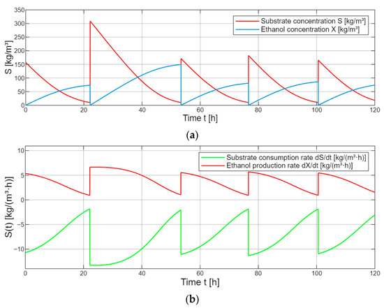
Figure 6.
Simulation graph of substrate and ethanol during the multiple fermentation process: (a) substrate (S) and ethanol (X) concentrations vs. time [kg/m3]; (b) through substrate consumption/production rates.
Figure 7 shows a single uninterrupted batch fermentation cycle over 46 h with an initial substrate concentration of and Monod kinetics as specified in the simulation environment. The top panel shows and . The red curve declines monotonically, with the rate of decline slowing as the substrate is depleted. The blue curve rises towards an asymptote as the conversion proceeds and approaches a plateau when is nearly exhausted. This behavior is consistent with the expected course of a batch fermentation without replenishment. The lower panel shows and . The magnitude of is greatest at the beginning, when the driving concentration is high, and then decreases as the process nears completion. The production rate increases to a peak during the most active metabolic phase and then decreases as the substrate becomes limiting.
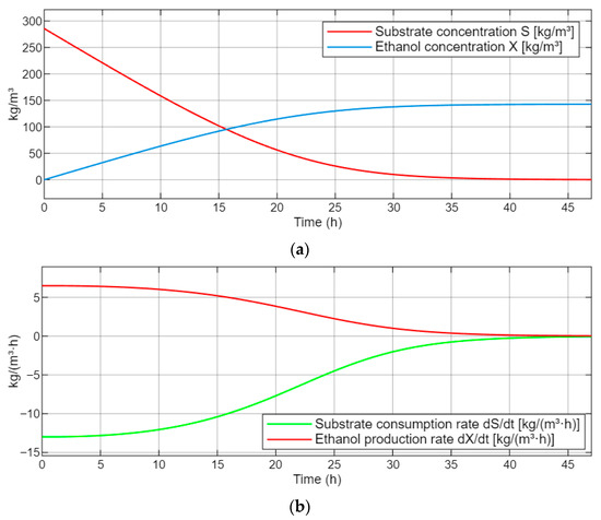
Figure 7.
Simulation graph of a 46 h alcoholic fermentation process with an initial substrate concentration of ; (a) substrate (S) and ethanol (X) concentrations vs. time [kg/m3]; (b) through substrate consumption/production rates.
Taken together, the results in Figure 6 and Figure 7 validate the simulation workflow. The repeated batch scenario demonstrates robust interaction between imaging-informed state updates and process kinetics. The single batch scenario confirms that the parameterization reproduces classical batch behavior under Monod dependence. Both cases show smooth evolution of concentrations and derivatives, predictable responses to the threshold rule, and consistency with mass balance expectations, which supports the use of the model for analysis and prospective decision support in controlled fermentation studies.
3.2. Validation of the Alcohol Fermentation Monitoring Model
The validation pathway begins with a simplified simulation of the real fermentation course implemented in Simulink and summarized in Figure 8. This configuration reproduces the time evolution of substrate and ethanol by combining a matrix of precomputed electrical impedance tomography reconstructions with a predefined time law governing the evolution of process parameters. In contrast to the dynamic Monod-based simulator presented earlier, which advances the state by integrating differential equations, the validation model prescribes concentrations directly as functions of time and uses the images as a consistent background for visualization and parameter readout. The MATLAB Function block marked as updateReconstruction receives simulation time and the reconstruction matrix and returns the current pair of concentrations for substrate and ethanol. The sigma_table variable provided from the MATLAB base workspace contains EIT reconstructions performed at specific time intervals during the 46 h fermentation process under study.
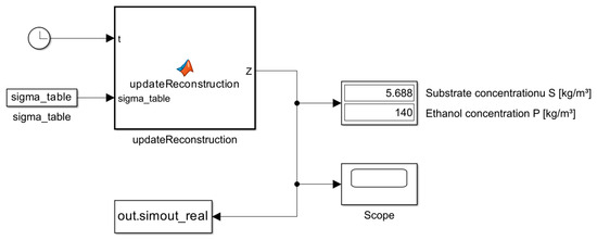
Figure 8.
Schematic Simulink model of the actual course of the alcoholic fermentation process.
Quantitative validation proceeds in two steps. First, an analytical reference trajectory is generated by an exponential law for substrate decay and by a mass balance for ethanol formation as implemented in the update block. The substrate follows (3)
with and over a window of approximately forty-six hours. The ethanol is computed from the mass balance (4)
with yield . These expressions define the reference pair of time series used for comparison and for driving the simplified simulator shown in Figure 8.
Second, the analytical profiles are confronted with concentrations recovered from real electrical impedance tomography measurements. A direct comparison between analytical simulation and experimental recovery is presented in Figure 9. The dashed red and blue curves show the simulated reference, and the red and blue markers show the values inferred from electrical impedance tomography. The agreement is close in both shape and scale. Early time differences are small and can be explained by mixing transients and local heterogeneity in conductivity. Late time differences are also small and are consistent with the finite spatial resolution of the reconstruction and with the decreasing signal-to-noise ratio as conductivity gradients shrink. The overall match supports the adopted conductivity to concentration calibration and confirms that the simplified simulator is an adequate reference for validating the monitoring pipeline.
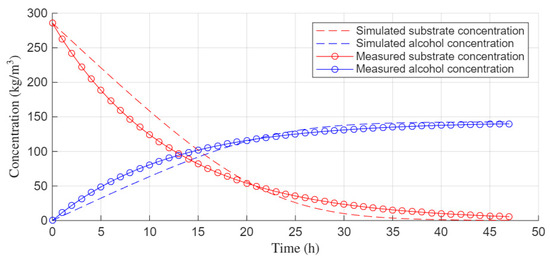
Figure 9.
Comparison of the 46 h alcoholic fermentation process between simulations and actual EIT measurements.
It should be emphasized that the substrate and ethanol concentration values presented in Figure 9 were not measured using reference methods. The term “actual measurements” refers to EIT tomographic electrical conductivity quantifications performed during a 46 h alcoholic fermentation process. Each measurement point on the graph represents the conversion of a 2502-element tomographic reconstruction vector (sigma) to the corresponding chemical concentrations using a calibration function. The regularity of the point pattern results from the nature of the conversion method used and the spatial averaging inherent in tomographic measurements. EIT measures averaged conductivity across the entire reactor volume, which naturally reduces local fluctuations and measurement noise typical of point-based analytical methods. It should be emphasized that the measurement points presented in Figure 9 represent averaged values across the entire reactor volume, which significantly reduces the influence of local fluctuations and measurement noise.
Figure 10 shows a sequence of 12 tomographic reconstructions of the tested reactor taken during a 46 h fermentation process. Reconstruction (a) was taken at the beginning of the process, while reconstruction (l) was taken at its completion. The sequence reveals a progressive redistribution of conductivity consistent with sugar depletion and ethanol formation. Color images adapted to human perception are for informational purposes only. The numerical values of the output vector are important for the process control system. Based on these values, the algorithm can estimate substrate concentrations. The varied colors confirm that the imaging layer provides stable and interpretable inputs to the concentration estimation step.
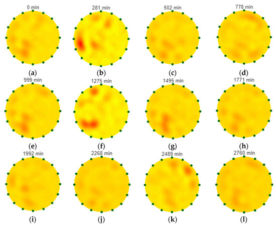
Figure 10.
Sequence of tomographic cross-sections acquired during a 46 h fermentation. Reconstructions (a–l) show successive time points in minutes from the process start (t = 0).
We evaluated computational performance on an Asus TUF laptop with an AMD Ryzen 7 5800H CPU at 3.2 GHz, 16 GB RAM, and an NVIDIA GeForce RTX 3060 with 6.4 GB VRAM running Windows 11. For the 16-electrode protocol at 1 kHz, one full EIT frame required 28–34 ms with GPU inference and 90–110 ms with CPU-only execution. The control layer added 20–30 ms from feature extraction through Monod model update to command dispatch. The end-to-end latency measured from the last voltage sample to actuation was 55–70 ms with the GPU enabled and 130–150 ms on CPU only, providing stable real-time operation at approximately 10–15 Hz with the GPU and 5–7 Hz on CPU. In practice, the system runs on any recent 64-bit machine with at least a quad-core CPU and 8 GB RAM, while a CUDA-capable GPU with 4 GB or more VRAM is recommended to reach the higher update rates.
3.3. Energy Accounting for EIT-Supervised Fermentation: Models and Results
Below, the energetic implications of coupling EIT-based state estimation with phase-aware temperature targeting are quantified. Building on the previously introduced kinetic core and conductivity-to-concentration calibration, a control-energy surrogate is derived that links setpoint trajectories to compressor and agitation loads via a temperature-lift–dependent COP, passive (free) cooling, and a cube-law model of mixing. An EIT-supervised strategy—whose targets are confined to admissible, phase-dependent temperature bands and biased toward ambient—is then compared with three traditional programs (constant, linear, exponential) over a 46 h batch. The resulting time profiles of instantaneous electric power, target temperatures with bands, and metabolic heat release are integrated to obtain cumulative energy, thereby allowing the specific contributions of supervision, free cooling, and reduced mixing to the observed savings to be isolated.
Figure 11 aggregates the dynamic response of four temperature control strategies over a 46 h alcoholic fermentation and the underlying metabolic drive, using the same color code across panels (EIT-supervised—blue, constant 25 °C—red, linear—green, exponential—magenta). In the top panel (“Instantaneous Electric Power”), each curve represents the total electric load , where compressor (cooling) electric power [W] and agitator/mixer electric power [W].
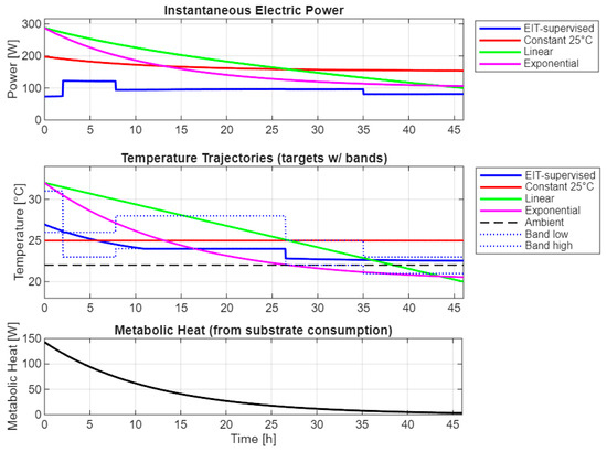
Figure 11.
Instantaneous power, temperature targets, and metabolic heat under EIT-supervised vs. traditional control.
For the EIT-supervised case (blue), cooling is dispatched only when tomographic state estimation indicates that temperature would leave a phase-dependent admissible band, and mixing setpoints are reduced outside the peak metabolic phase. Consequently, the blue power trace exhibits short plateaus and long low-duty intervals. In the three traditional setpoint programs, agitation is kept constant while the cooling duty decays mainly because the commanded temperature gradually approaches the ambient. The 25 °C hold declines the slowest (red), the linear ramp declines linearly (green), and the exponential target produces a concave decay (magenta). Cooling power in all cases is computed with a temperature-lift-dependent coefficient of performance (COP) and a “free-cooling” term that removes heat to ambient without compressor work when permissible, i.e.,
where: —coefficient of performance of the refrigeration cycle [–], depends on the temperature lift, —lower bound of the COP [–], —nominal COP intercept (for negligible lift) [–], —COP degradation coefficient per kelvin of lift [K−1], —broth (process) temperature [°C or K], —coolant or jacket-side temperature used in the lift [°C or K] (often cooling-water supply), —passive (“free-cooling”) heat rejected to the ambient without compressor work [W], —overall heat-transfer conductance (U × A) [W·K−1], —ambient air temperature [°C or K], —gross cooling duty before accounting for passive removal [W], —fractional coefficient (0–1) crediting metabolic heat against external cooling [–], —metabolic heat-release rate [W].
The mixing power follows a variable-frequency-drive cube law, , with lowered by the supervisor during lag and maturation. These relationships are part of the control-energy surrogate model and complement the kinetic core presented in the manuscript.
The middle panel in Figure 11, titled “Temperature Trajectories (targets w/ bands)”, shows the target temperature programs that feed the above power calculation. The three traditional strategies (red, green, magenta) are predefined setpoints. By contrast, the EIT-supervised trajectory (solid blue) is constrained to remain between two dotted blue envelopes labeled “Band low” and “Band high”. In the code, these are Tband_lo and Tband_hi. They are phase-dependent admissible corridors inferred from the tomographically estimated state: EIT reconstructions are converted to concentrations via a calibrated map and propagated through a Monod kinetic core, which provides a smooth phase indicator (lag → early exponential → peak → late → maturation). The conductivity-to-concentration calibration and the Monod dependence used by the kinetic block, , with and , together with the associated rate equations , , and balances , , (Section 2 and Section 3), are employed. The analytical reference trajectory used in validation, with and , and (Equations (2)–(4) in the manuscript), is also provided. These elements underpin our phase logic and, therefore, the blue bands and the supervised temperature trace.
The bottom panel (“Metabolic Heat (from substrate consumption)”) depicts the driving heat release , which declines monotonically as substrate is depleted. In the kinetic core documented in the manuscript, rates follow Monod and stoichiometric yields. For the energy accounting used here, we map the consumption rate to heat release via the surrogate which is consistent with the simulated behavior of and reported in the validation figures (the magnitude of is the largest early and decreases as the batch nears completion, while peaks at mid-run).
Figure 12 summarizes the integral energetic outcome. Each bar reports the 46 h electric energy .
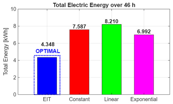
Figure 12.
Energy use comparison: EIT-supervised vs. traditional setpoints (46 h).
The EIT-supervised strategy (blue) attains the minimum (~4.35 kWh) because the supervisor biases the target toward ambient within the admissible corridor, which reduces temperature lift and increases COP, exploits free-cooling whenever to offload compressor work, and lowers agitation outside the peak metabolic window according to the cube law. The constant 25 °C hold (red, ~7.59 kWh) is penalized by sustained lift. The linear ramp (green, ~8.21 kWh) incurs high early-time duty when the setpoint is far from ambient, and the exponential program (magenta, ~6.99 kWh) moderates duty relative to linear but remains less efficient than EIT supervision because it ignores the real-time metabolic state reflected by EIT. Altogether, Figure 11 and Figure 12 illustrate how the EIT-driven pipeline (conductivity field → calibrated concentrations → Monod kinetics → phase-aware temperature bands) translates into lower instantaneous power and the best cumulative energy over the batch.
3.4. Sensitivity and Uncertainty Analysis of the Conductivity—Substrate Calibration Model
Figure 13 presents the sensitivity and uncertainty analysis of the linear calibration model that relates electrical conductivity (in arbitrary units [a.u.]) to substrate concentration during fermentation. Panel (A) shows the calibration curve obtained from experimental data, where measured conductivity values are plotted against analytically determined substrate concentrations. The solid black line represents the fitted linear model described by the equation , while the dashed and dotted lines indicate the 95% confidence interval (CI) and 95% prediction interval (PI), respectively. The color of the data points corresponds to the process temperature (T), highlighting its relatively minor variation during the experiment. The linearity of the relationship confirms that conductivity can be used as a reliable proxy for substrate concentration within the tested range.
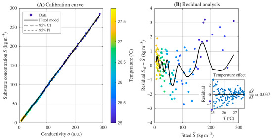
Figure 13.
Sensitivity and uncertainty analysis of the linear calibration between conductivity and substrate concentration: (A)—calibration curve for , (B)—residual analysis with temperature-related bias visualization.
Panel (B) provides a residual analysis to assess model robustness and to visualize temperature-related effects. The residuals, defined as are plotted against the fitted values, where denotes the reference substrate concentration and the model estimate. The black curve represents a locally weighted LOESS regression, showing small systematic deviations that suggest minor nonlinearity at the extremes of the range. The inset plot, labeled “Temperature effect,” depicts the residuals as a function of temperature T [°C] and shows a weak positive slope, approximately [kg m−3 °C−1], indicating that conductivity slightly increases with temperature. Together, these panels demonstrate that the calibration model provides accurate concentration estimates with limited temperature sensitivity and acceptable uncertainty for process monitoring applications.
Figure 14 summarizes the Monte Carlo uncertainty decomposition for the linear conductivity–substrate calibration at a representative operating point of kg . The bar chart reports the standard uncertainty contributed by temperature variation, measurement noise, and electrode drift, together with the combined effect. Temperature dominates with an estimated 3.00 kg one-sigma contribution, followed by measurement noise at 1.50 kg and electrode drift at 0.76 kg , yielding a combined standard uncertainty of 3.45 kg . These values were obtained using a physically plausible disturbance model that assumes approximately 1 °C one-sigma temperature variability with a 2% per °C conductivity coefficient, 1% measurement noise, and 0.5% slow electrode drift, which reflects the operating window of our experiments. Expressed relatively, the combined uncertainty corresponds to about 2.3% at kg and about 1.2% of the initial concentration kg , indicating that the calibration maintains sufficient precision for closed-loop supervision and event-triggered control. The figure complements the calibration and residual analyses by quantifying how each disturbance source propagates to concentration estimates and by confirming that the overall uncertainty remains small compared with typical decision thresholds used in our control logic.
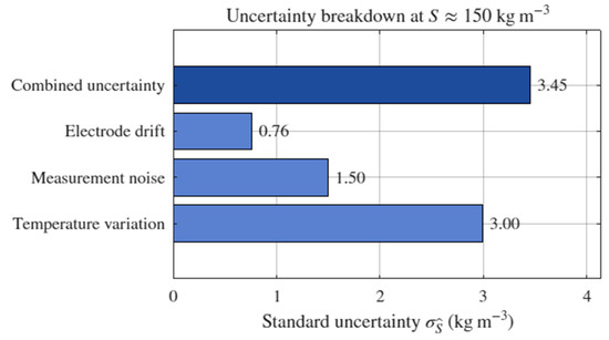
Figure 14.
Uncertainty breakdown of the conductivity–substrate calibration.
4. Discussion
The study demonstrates an AI-enhanced monitoring pipeline for alcoholic fermentation that couples electrical impedance tomography with a residual convolutional network from the ResNet family and a Monod-based kinetic core to estimate substrate and ethanol and to enable short-range prediction. The approach is consistent with the recent progress in deep learning for electrical impedance tomography reconstruction and with reviews that document the ill-posed nature of the inverse problem and the value of data-driven priors [24,35,36].
The sensing layer builds on the use of impedance-based measurements in bioprocess monitoring, where noninvasive electrical methods track biomass and composition during fermentation. Evidence for feasibility is provided by demonstrations of electrochemical impedance spectroscopy in microbial cultivations and by reports that impedance spectroscopy can follow biomass in complex broths [37,38,39].
Validation uses analytical reference trajectories grounded in standard Monod-style modeling of ethanol fermentation and a mass balance for the product. The observed agreement between analytical references and concentrations recovered from electrical impedance tomography aligns with recent kinetic studies of ethanol production that employ unstructured models in batch and fed-batch regimes. Early deviations can be ascribed to mixing transients and spatial heterogeneity, and late deviations are compatible with the known resolution and signal-to-noise limits of electrical impedance tomography [40,41].
The batch course reported here is consistent with the established physiology of Saccharomyces cerevisiae where rapid early sugar uptake is followed by ethanol accumulation and rate deceleration under substrate depletion and product stress. The broader literature documents cellular responses that underpin ethanol tolerance and membrane level adaptations during ethanol challenge and these mechanisms explain the observed turning points of the trajectories [42,43].
The sensitivity of fermentation kinetics to nitrogen availability is well described by controlled studies and reviews that resolve effects of both level and timing of yeast assimilable nitrogen. The stable mapping from impedance signals to concentration estimates observed here is therefore coherent with scenarios where nitrogen regimes modulate rates and product formation while the electrical pathway offers a continuous surrogate for state estimation [44,45,46].
The methodological choice to pair electrical impedance tomography with a residual convolutional reconstructor follows current practice in imaging-guided state estimation and is supported by surveys that compare single-network reconstruction and hybrid strategies for this modality. The stability of the repeated batch regime with an event-triggered refresh is consistent with the view that imaging-informed signals can support supervisory control and scheduling in bioethanol processes within the accuracy bounds of modern electrical impedance tomography [24,36].
The proposed AI-enhanced sensing and estimation enables supervisory scheduling of electricity use in fermentation and is consistent with evidence that process industries can supply demand-side flexibility to support grids with variable renewable generation [47]. Brewery and fermentation sites carry significant electric loads in refrigeration and agitation, and refrigeration is often the dominant electrical consumer that can be time shifted without compromising product quality when process constraints are respected. The event-triggered threshold and cooldown logic provide actionable signals to shift cooling and pumping toward low price or high renewable periods, while machine learning based bioprocess monitoring supports real-time decision making [48]. When co-located with biogas units, additional flexibility can be provided because modern biogas plants can modulate output in response to market conditions and renewable variability [49]. Digitization of these functions should follow established guidance for operational technology security to maintain resilience of scheduling and control [50].
Taken together, the results indicate that an imaging-informed AI pipeline can deliver reliable state estimation and short-range prediction for alcoholic fermentation under realistic variability, with observed deviations consistent with known limits of electrical impedance tomography and process mixing. The approach enables energy-aware supervision in which cooling and agitation are scheduled against price signals and renewable availability, and it can be extended where fermentation is co-located with bioenergy units.
Measurement noise, electrode drift, and process disturbances are inherent challenges in EIT-based control systems and directly influence reconstruction stability and control reliability. Measurement noise primarily affects the voltage acquisition stage, introducing random fluctuations that propagate through the inverse problem and can cause small but noticeable variations in reconstructed conductivity maps. These effects are mitigated through the use of averaging filters, regularization, and deep learning based reconstruction models, such as the ResNet50 applied in this work, which are inherently robust to high-frequency noise. Electrode drift and polarization introduce low-frequency systematic errors, particularly during long-term experiments, leading to gradual baseline shifts in reconstructed conductivity. This issue is alleviated through periodic impedance calibration, temperature compensation, and the use of non-polarizable electrodes. Process disturbances such as mixing inhomogeneities, gas bubble formation, or thermal gradients can transiently distort the electric field distribution and thus perturb the reconstructed conductivity. The control algorithm mitigates these effects through temporal smoothing of feature vectors and event-triggered decision logic, ensuring that control actions are based on stable trends rather than instantaneous fluctuations. Overall, the combined use of noise-tolerant reconstruction, adaptive calibration, and disturbance-aware control logic provides sufficient stability for reliable closed-loop operation under realistic industrial conditions.
Beyond the controlled laboratory conditions, the framework is designed to remain robust under typical industrial disturbances by combining sensing-layer compensation with disturbance-aware decision logic. Sudden temperature excursions are handled through continuous multi-point temperature monitoring and compensation in the conductivity→concentration mapping, with supervisory guards that delay actuation and trigger rapid re-baselining if deviations exceed preset limits. Electrode fouling and polarization are managed by periodic impedance checks and baseline tracking. The estimator updates gain/offset terms online and can switch to a diagnostic mode that suspends control actions when quality indicators (e.g., reconstruction consistency and residual thresholds) degrade, which addresses confounders known for EIT in industrial media. At the control layer, temporal smoothing, hysteresis, and a cooldown mechanism ensure that state estimates must remain stable over a dwell time before any actuation is issued, preventing spurious responses to transient artefacts caused by bubbles, mixing inhomogeneities, or drift. Together, these measures provide a fail-safe operating envelope in which the system either adapts to disturbances or reverts to safe monitoring until recalibration or maintenance restores nominal conditions.
Key limitations of the model include simplified kinetic assumptions, the scale and geometry of the experimental rig, and the specificity of the calibration. In the baseline configuration, the Monod-type kinetic core adopts simplified assumptions—biomass and ethanol concentrations are held fixed at 105 kg·m−3 and 0 kg·m−3, respectively—which reduces model fidelity with respect to coupled metabolic dynamics, product inhibition and nutrient-driven physiological changes that commonly occur in industrial fermentations. The experimental validation was performed in a bench-scale 3.5 L tank reactor with a fixed electrode geometry and repeatable stirring. Such a small, well-mixed tank does not fully reproduce the mixing patterns, heat transfer characteristics, and three-dimensional flow structures of industrial-scale fermenters, and the model’s assumption of homogeneous conditions after mixing therefore underestimates the spatial heterogeneity often present in production reactors. These advances would position fermentation as a flexible demand resource that supports stable and efficient operation of renewable integrated power systems.
5. Conclusions
The motivation for using Electrical Impedance Tomography (EIT) in closed-loop process control lies in its ability to transform raw boundary measurements into a spatially resolved representation of the process interior by solving the tomographic inverse problem. The reconstruction yields a pixelwise conductivity map, where each pixel is associated with a well-defined spatial location. This representation can be conveniently expressed as a numerical output vector whose component order encodes the spatial distribution of process variables. Such a vector can be further processed in a deterministic or data-driven manner—using statistical inference, fuzzy logic, or machine learning—to estimate key control parameters, including substrate concentrations, ion content (pH), or biomass levels. These quantities form the basis for control actions such as adjusting feed rates, mixing intensity, or temperature setpoints. Importantly, without the intermediate tomographic reconstruction step, direct measurement signals alone would provide only aggregated or localized information and would be insufficient to achieve comparable spatial resolution and estimation accuracy. EIT thus enables the transition from conventional point-based monitoring to full-field, model-based control, supporting automation and facilitating operation under Industry 4.0 and AI-enhanced paradigms.
The adoption of EIT as a core sensing modality fundamentally expands the capabilities of process automation, making it possible to achieve high-fidelity, real-time state estimation that is both robust and scalable. This paradigm supports the development of self-optimizing, unattended control systems capable of dynamically responding to process disturbances and external energy signals. As a result, EIT-based solutions offer a promising pathway toward improving process efficiency, reducing energy consumption, and enabling more sustainable and resilient industrial operations—objectives that are particularly relevant in the era of renewable energy integration and distributed energy management.
Author Contributions
Conceptualization, K.K. and T.R.; methodology, G.K., T.R. and K.K.; software, K.K. and T.R.; validation, K.G., E.G. and A.S.; resources, T.R.; data curation, T.R. and G.K.; writing—original draft preparation, M.K. and G.K.; writing—review and editing, T.R., M.K., K.G., E.G. and A.S.; visualization, K.K. and G.K.; supervision, T.R.; funding acquisition, T.R. All authors have read and agreed to the published version of the manuscript.
Funding
This research received no external funding.
Data Availability Statement
The data presented in this study are available on request from the corresponding author. The data is not made public because it is the property of the company.
Conflicts of Interest
Authors Krzysztof Król and Tomasz Rymarczyk were employed by the company Research and Development Center, Netrix S.A. The remaining authors declare that the research was conducted in the absence of any commercial or financial relationships that could be construed as a potential conflict of interest.
Abbreviations
The following abbreviations are used in this manuscript:
| AI | Artificial Intelligence |
| a.u. | arbitrary units |
| ATP | adenosine 5′-triphosphate |
| CMOS | Complementary Metal Oxide Semiconductor |
| ECT | Electrical Capacitance Tomography |
| EIT | Electrical Impedance Tomography |
| FEM | Finite Element Method |
| GPU | Graphics Processing Unit |
| LCD | Liquid Crystal Display |
| MLOps | Machine Learning Operations |
| MRI | Magnetic Resonance Imaging |
| NIR | Near Infrared Spectroscopy |
| NMR | Nuclear Magnetic Resonance |
| OCT | Optical Coherence Tomography |
| PAT | Process Analytical Technology |
| RJ-45 | Registered Jack 45 |
| RMSE | Root Mean Square Error |
| UST | Ultrasound Tomography |
| UV-Vis | Ultraviolet Visible Spectroscopy |
References
- Su, Q.; Ganesh, S.; Moreno, M.; Bommireddy, Y.; Gonzalez, M.; Reklaitis, G.V.; Nagy, Z.K. A Perspective on Quality-by-Control (QbC) in Pharmaceutical Continuous Manufacturing. Comput. Chem. Eng. 2019, 125, 216–231. [Google Scholar] [CrossRef]
- Gerzon, G.; Sheng, Y.; Kirkitadze, M. Process Analytical Technologies—Advances in Bioprocess Integration and Future Perspectives. J. Pharm. Biomed. Anal. 2022, 207, 114379. [Google Scholar] [CrossRef] [PubMed]
- Bowler, A.L.; Bakalis, S.; Watson, N.J. A Review of In-Line and on-Line Measurement Techniques to Monitor Industrial Mixing Processes. Chem. Eng. Res. Des. 2020, 153, 463–495. [Google Scholar] [CrossRef]
- Hong, C.Y.; Zhang, Y.F.; Zhang, M.X.; Leung, L.M.G.; Liu, L.Q. Application of FBG Sensors for Geotechnical Health Monitoring, a Review of Sensor Design, Implementation Methods and Packaging Techniques. Sens. Actuators A Phys. 2016, 244, 184–197. [Google Scholar] [CrossRef]
- Roberts, J.; Power, A.; Chapman, J.; Chandra, S.; Cozzolino, D. The Use of UV-Vis Spectroscopy in Bioprocess and Fermentation Monitoring. Fermentation 2018, 4, 18. [Google Scholar] [CrossRef]
- Kulisz, M.; Kłosowski, G.; Rymarczyk, T.; Hoła, A.; Niderla, K.; Sikora, J. The Use of the Multi-Sequential LSTM in Electrical Tomography for Masonry Wall Moisture Detection. Measurement 2024, 234, 114860. [Google Scholar] [CrossRef]
- Kłosowski, G.; Rymarczyk, T.; Niderla, K.; Kulisz, M.; Skowron, Ł.; Soleimani, M. Using an LSTM Network to Monitor Industrial Reactors Using Electrical Capacitance and Impedance Tomography—A Hybrid Approach. Eksploat. I Niezawodn. Maint. Reliab. 2023, 25, 2023. [Google Scholar] [CrossRef]
- Przysucha, B.; Wójcik, D.; Rymarczyk, T.; Król, K.; Kozłowski, E.; Gąsior, M. Analysis of Reconstruction Energy Efficiency in EIT and ECT 3D Tomography Based on Elastic Net. Energies 2023, 16, 1490. [Google Scholar] [CrossRef]
- Koulountzios, P.; Rymarczyk, T.; Soleimani, M. Ultrasonic Time-of-Flight Computed Tomography for Investigation of Batch Crystallisation Processes. Sensors 2021, 21, 639. [Google Scholar] [CrossRef] [PubMed]
- Ultrasound Tomography for Control of Batch Crystallization—The University of Bath’s Research Portal. Available online: https://researchportal.bath.ac.uk/en/studentTheses/ultrasound-tomography-for-control-of-batch-crystallization (accessed on 25 August 2025).
- Ziolkowski, M.; Gratkowski, S.; Zywica, A.R. Analytical and Numerical Models of the Magnetoacoustic Tomography with Magnetic Induction. COMPEL—Int. J. Comput. Math. Electr. Electron. Eng. 2018, 37, 538–548. [Google Scholar] [CrossRef]
- Gocławski, J.; Sekulska-Nalewajko, J.; Korzeniewska, E. Prediction of Textile Pilling Resistance Using Optical Coherence Tomography. Sci. Rep. 2022, 12, 1–15. [Google Scholar] [CrossRef]
- Korzeniewska, E.; Gałązka-Czarnecka, I.; Sekulska-Nalewajko, J.; Gocławski, J.; Dróźdż, T.; Kiełbasa, P. Assessment of Changes in Vitamin Content and Morphological Characteristics in Strawberries Modified with a Pulsed Electric Field Using Chromatography and Optical Coherence Tomography. NFS J. 2025, 38, 100217. [Google Scholar] [CrossRef]
- Hlava, J.; Abouelazayem, S. Control Systems with Tomographic Sensors—A Review. Sensors 2022, 22, 2847. [Google Scholar] [CrossRef] [PubMed]
- Hampel, U.; Babout, L.; Banasiak, R.; Schleicher, E.; Soleimani, M.; Wondrak, T.; Vauhkonen, M.; Lähivaara, T.; Tan, C.; Hoyle, B.; et al. A Review on Fast Tomographic Imaging Techniques and Their Potential Application in Industrial Process Control. Sensors 2022, 22, 2309. [Google Scholar] [CrossRef]
- Hollenberg, M.; Liebing, T.; Kern, T.A.; Kähler, D. Simulation Framework for Electrical Impedance Tomography Systems. Meas. Sens. 2025, 38, 101416. [Google Scholar] [CrossRef]
- Rao, G.; Aghajanian, S.; Koiranen, T.; Wajman, R.; Jackowska-Strumiłło, L. Process Monitoring of Antisolvent Based Crystallization in Low Conductivity Solutions Using Electrical Impedance Spectroscopy and 2-D Electrical Resistance Tomography. Appl. Sci. 2020, 10, 3903. [Google Scholar] [CrossRef]
- Yan, R.; Viumdal, H.; Mylvaganam, S. Process Tomography for Model Free Adaptive Control (MFAC) via Flow Regime Identification in Multiphase Flows. IFAC-Pap. 2020, 53, 11753–11760. [Google Scholar] [CrossRef]
- Yang, C.; Cui, Z.; Xue, Q.; Wang, H.; Zhang, D.; Geng, Y. Application of a High Speed ECT System to Online Monitoring of Pneumatic Conveying Process. Measurement 2014, 48, 29–42. [Google Scholar] [CrossRef]
- Metcalfe, B.; Acosta-Pavas, J.C.; Robles-Rodriguez, C.E.; Georgakilas, G.K.; Dalamagas, T.; Aceves-Lara, C.A.; Daboussi, F.; Koehorst, J.J.; Corrales, D.C. Towards a Machine Learning Operations (MLOps) Soft Sensor for Real-Time Predictions in Industrial-Scale Fed-Batch Fermentation. Comput. Chem. Eng. 2025, 194, 108991. [Google Scholar] [CrossRef]
- Wu, D.; Xu, Y.; Xu, F.; Shao, M.; Huang, M. Machine Learning Algorithms for In-Line Monitoring during Yeast Fermentations Based on Raman Spectroscopy. Vib. Spectrosc. 2024, 132, 103672. [Google Scholar] [CrossRef]
- Feng, Y.; Tian, X.; Chen, Y.; Wang, Z.; Xia, J.; Qian, J.; Zhuang, Y.; Chu, J. Real-Time and on-Line Monitoring of Ethanol Fermentation Process by Viable Cell Sensor and Electronic Nose. Bioresour. Bioprocess. 2021, 8, 1–10. [Google Scholar] [CrossRef] [PubMed]
- Kwon, H.; Shiu, J.; Rivera, E.C.; Yamakaya, C. Soft Sensor for Ethanol Fermentation Monitoring through Data-Driven Modeling and Synthetic Data Generation. In Proceedings of the 4th International Electronic Conference on Biosensors, Online, 20–22 May 2024; Volume 104, p. 30. [Google Scholar] [CrossRef]
- Zhang, T.; Tian, X.; Liu, X.C.; Ye, J.A.; Fu, F.; Shi, X.T.; Liu, R.G.; Xu, C.H. Advances of Deep Learning in Electrical Impedance Tomography Image Reconstruction. Front. Bioeng. Biotechnol. 2022, 10, 1019531. [Google Scholar] [CrossRef]
- Tinôco, D.; Batista Da Silveira, W. Kinetic Model of Ethanol Inhibition for Kluyveromyces marxianus CCT 7735 (UFV-3) Based on the Modified Monod Model by Ghose & Tyagi. Biologia 2021, 76, 3511–3519. [Google Scholar] [CrossRef]
- Rzasa, M.; Łukasiewicz, E.; Wójtowicz, D. Test of a New Low-Speed Compressed Air Engine for Energy Recovery. Energies 2021, 14, 1179. [Google Scholar] [CrossRef]
- Urry, L.A.; Cain, M.L.; Wasserman, S.A.; Minorsky, P.V.; Orr, R. Biologia Campbella, 12th ed.; REBIS: Poznań, Poland, 2025. [Google Scholar]
- Yadav, M.; Yadav, H.S. Biochemistry: Fundamentals and Bioenergetics; Bentham Science Publisher: Sharjah, United Arab Emirates, 2021; Volume 418. [Google Scholar]
- Ji, X.X.; Zhang, Q.; Yang, B.X.; Song, Q.R.; Sun, Z.Y.; Xie, C.Y.; Tang, Y.Q. Response Mechanism of Ethanol-Tolerant Saccharomyces cerevisiae Strain ES-42 to Increased Ethanol during Continuous Ethanol Fermentation. Microb. Cell Fact. 2025, 24, 1–15. [Google Scholar] [CrossRef]
- Wolf, I.R.; Marques, L.F.; de Almeida, L.F.; Lázari, L.C.; de Moraes, L.N.; Cardoso, L.H.; Alves, C.C.d.O.; Nakajima, R.T.; Schnepper, A.P.; Golim, M.d.A.; et al. Integrative Analysis of the Ethanol Tolerance of Saccharomyces cerevisiae. Int. J. Mol. Sci. 2023, 24, 5646. [Google Scholar] [CrossRef]
- Christofi, S.; Papanikolaou, S.; Dimopoulou, M.; Terpou, A.; Cioroiu, I.B.; Cotea, V.; Kallithraka, S. Effect of Yeast Assimilable Nitrogen Content on Fermentation Kinetics, Wine Chemical Composition and Sensory Character in the Production of Assyrtiko Wines. Appl. Sci. 2022, 12, 1405. [Google Scholar] [CrossRef]
- Tse, T.J.; Wiens, D.J.; Reaney, M.J.T. Production of Bioethanol—A Review of Factors Affecting Ethanol Yield. Fermentation 2021, 7, 268. [Google Scholar] [CrossRef]
- IEEE Std 802.3-2002 (Revision of IEEE Std 802.3, 2000 edn); 802.3-2022—IEEE Standard for Information technology-Telecommunications and Information Exchange Between Systems-Local and Metropolitan Area Networks-Specific Requirements Part 3: Carrier Sense Multiple Access with Collision Detection (CSMA/CD) Access Method and Physical Layer Specifications. IEEE: New York, NY, USA, 2002; pp. 1–1550. [CrossRef]
- Konopacka, A.; Konopacki, M.; Kordas, M.; Rakoczy, R. Mathematical Modeling of Ethanol Production by Saccharomyces cerevisiae in Batch Culture with Non-Structured Model. Chem. Process Eng. 2023, 40, 281–291. [Google Scholar] [CrossRef]
- Kulisz, M.; Kłosowski, G.; Rymarczyk, T.; Słoniec, J.; Gauda, K.; Cwynar, W. Optimizing the Neural Network Loss Function in Electrical Tomography to Increase Energy Efficiency in Industrial Reactors. Energies 2024, 17, 681. [Google Scholar] [CrossRef]
- Wang, J.; Deng, J.; Liu, D. Deep Prior Embedding Method for Electrical Impedance Tomography. Neural Netw. 2025, 188, 107419. [Google Scholar] [CrossRef]
- Slouka, C.; Wurm, D.J.; Brunauer, G.; Welzl-Wachter, A.; Spadiut, O.; Fleig, J.; Herwig, C. A Novel Application for Low Frequency Electrochemical Impedance Spectroscopy as an Online Process Monitoring Tool for Viable Cell Concentrations. Sensors 2016, 16, 1900. [Google Scholar] [CrossRef] [PubMed]
- Díaz Pacheco, A.; Delgado-Macuil, R.J.; Larralde-Corona, C.P.; Dinorín-Téllez-Girón, J.; Martínez Montes, F.; Martinez Tolibia, S.E.; López y López, V.E. Two-Methods Approach to Follow up Biomass by Impedance Spectroscopy: Bacillus Thuringiensis Fermentations as a Study Model. Appl. Microbiol. Biotechnol. 2022, 106, 1097–1112. [Google Scholar] [CrossRef]
- Díaz Pacheco, A.; Dinorín-Téllez-Girón, J.; Martínez Montes, F.J.; Martínez Tolibia, S.E.; López y López, V.E. On-Line Monitoring of Industrial Interest Bacillus Fermentations, Using Impedance Spectroscopy. J. Biotechnol. 2022, 343, 52–61. [Google Scholar] [CrossRef]
- Salakkam, A.; Phukoetphim, N.; Laopaiboon, P.; Laopaiboon, L. Mathematical Modeling of Bioethanol Production from Sweet Sorghum Juice under High Gravity Fermentation: Applicability of Monod-Based, Logistic, Modified Gompertz and Weibull Models. Electron. J. Biotechnol. 2023, 64, 18–26. [Google Scholar] [CrossRef]
- Veloso, I.I.K.; Rodrigues, K.C.S.; Batista, G.; Cruz, A.J.G.; Badino, A.C. Mathematical Modeling of Fed-Batch Ethanol Fermentation Under Very High Gravity and High Cell Density at Different Temperatures. Appl. Biochem. Biotechnol. 2022, 194, 2632–2649. [Google Scholar] [CrossRef] [PubMed]
- Lairón-Peris, M.; Routledge, S.J.; Linney, J.A.; Alonso-del-Real, J.; Spickett, C.M.; Pitt, A.R.; Guillamón, J.M.; Barrio, E.; Goddard, A.D.; Querol, A. Lipid Composition Analysis Reveals Mechanisms of Ethanol Tolerance in the Model Yeast Saccharomyces cerevisiae. Appl. Environ. Microbiol. 2021, 87, 1–22. [Google Scholar] [CrossRef] [PubMed]
- Sahana, G.R.; Balasubramanian, B.; Joseph, K.S.; Pappuswamy, M.; Liu, W.C.; Meyyazhagan, A.; Kamyab, H.; Chelliapan, S.; Joseph, B.V. A Review on Ethanol Tolerance Mechanisms in Yeast: Current Knowledge in Biotechnological Applications and Future Directions. Process Biochem. 2024, 138, 1–13. [Google Scholar] [CrossRef]
- Cairns, P.; Hamilton, L.; Racine, K.; Phetxumphou, K.; Ma, S.; Lahne, J.; Gallagher, D.; Huang, H.; Moore, A.N.; Stewart, A.C. The Science of Beer Effects of Hydroxycinnamates and Exogenous Yeast Assimilable Nitrogen on Cider Aroma and Fermentation Performance Effects of Hydroxycinnamates and Exogenous Yeast Assimilable Nitrogen on Cider Aroma and Fermentation Performance. J. Am. Soc. Brew. Chem. 2021, 2022, 236–247. [Google Scholar] [CrossRef]
- Godillot, J.; Sanchez, I.; Perez, M.; Picou, C.; Galeote, V.; Sablayrolles, J.M.; Farines, V.; Mouret, J.R. The Timing of Nitrogen Addition Impacts Yeast Genes Expression and the Production of Aroma Compounds During Wine Fermentation. Front. Microbiol. 2022, 13, 829786. [Google Scholar] [CrossRef]
- Li, J.; Yuan, M.; Meng, N.; Li, H.; Sun, J.; Sun, B. Influence of Nitrogen Status on Fermentation Performances of Non-Saccharomyces Yeasts: A Review. Food Sci. Hum. Wellness 2024, 13, 556–567. [Google Scholar] [CrossRef]
- Golmohamadi, H. Demand-Side Management in Industrial Sector: A Review of Heavy Industries. Renew. Sustain. Energy Rev. 2022, 156, 111963. [Google Scholar] [CrossRef]
- Sharma, D.; Singh, K. AI-Enhanced Bioprocess Technologies: Machine Learning Implementations from Upstream to Downstream Operations. World J. Microbiol. Biotechnol. 2025, 41, 1–29. [Google Scholar] [CrossRef] [PubMed]
- Dotzauer, M. Determining Optimal Component Configurations for Flexible Biogas Plants Based on Power Prices of 2020–2022 and the Legislation Framework in Germany. Renew Energy 2024, 236, 121252. [Google Scholar] [CrossRef]
- Stouffer, K.; Pease, M.; Tang, C.; Zimmerman, T.; Pillitteri, V.; Lightman, S.; Hahn, A.; Saravia, S.; Sherule, A.; Thompson, M. Guide to Operational Technology (OT) Security. 2023. Available online: https://nvlpubs.nist.gov/nistpubs/SpecialPublications/NIST.SP.800-82r3.pdf (accessed on 6 October 2025). [CrossRef]
Disclaimer/Publisher’s Note: The statements, opinions and data contained in all publications are solely those of the individual author(s) and contributor(s) and not of MDPI and/or the editor(s). MDPI and/or the editor(s) disclaim responsibility for any injury to people or property resulting from any ideas, methods, instructions or products referred to in the content. |
© 2025 by the authors. Licensee MDPI, Basel, Switzerland. This article is an open access article distributed under the terms and conditions of the Creative Commons Attribution (CC BY) license (https://creativecommons.org/licenses/by/4.0/).