Risk-Based Decision Modelling for Wind Turbine Leading Edge Erosion

Abstract

IEA Wind Task 43 seeks to “unlock the full value of wind energy through digital transformation”. One mechanism to realize value is through enhanced data-driven decision-making and, while many areas in the wind sector can benefit from improved decision support, this case study focusses on a well-defined wind energy maintenance scenario involving blade inspection and repair. The solution concentrates on the specific damage category of blade leading edge erosion (LEE) and the optimum action to be taken for a given level of damage detected during periodic inspections. The key decision is whether to initiate repairs immediately or continue operating the turbine until the next inspection—and, if so, when that next inspection should take place. Even for such a specific damage type and decision option, the overall solution draws on multiple data types, ranging from damage classifications to cost drivers, and integrates a number of components including damage propagation, performance, and cost models. The core of the solution is a risk-based decision model using heuristic strategies, and Bayesian networks for optimized decision-making. This paper outlines the overall solution, expands on the data and modelling implementations, and discusses the results and conclusions arising from the investigation.

1. Introduction

Digitalization has the potential to reform activities like leading edge erosion (LEE) inspection and maintenance planning by leveraging inspection data, maintenance reports, operational data, and advanced modelling techniques to optimize decision-making. LEE is caused by the repeated impact of raindrops and airborne particles on the leading edge of wind turbine blades, resulting in initiation and progression of erosion damage. This degradation adversely affects aerodynamic performance, leading to reduced energy output. If left unaddressed, LEE can eventually compromise the structural integrity of the blades.

Early repairs can mitigate the negative effects of LEE on both turbine performance and blade durability, but they also incur additional costs. The decision of when to perform repairs involves a trade-off between direct repair costs—including production losses during downtime—and the ongoing revenue losses due to diminished aerodynamic efficiency. Optimal, risk-based decision-making seeks to minimize expected costs, including those associated with reduced energy production [1]. This approach supports decisions regarding the timing, type, and scope of inspections and repairs.

Evaluating such decisions requires predictive models that estimate the initiation and progression of damage over time, enabling assessment of the consequences of different maintenance strategies. This project explored the key steps in formulating decision objectives, identifying relevant datasets, developing and integrating predictive models, and evaluating decision outcomes.

The decision problem addressed in this study involves a wind farm owner/operator determining inspection and repair strategies for LEE. Periodically, during maintenance planning, turbines may be inspected using drones. If LEE is detected, repairs may be scheduled. The optimal strategy is derived using a decision model that incorporates turbine-specific data—such as power curves, rotor dimensions, and blade material properties—alongside site-specific statistical weather data, including probability distributions for wind speed, rainfall intensity, and droplet size.

The following section introduces approaches for decision modelling and provides the motivation for the approach applied in this study.

1.1. Decision-Making for Inspection and Repair

Inspection and repair optimization is a sequential decision problem under uncertainty [2]. According to Bayesian decision theory, optimal decisions maximize expected utility or minimize lifecycle costs [3]. While optimal solutions exist once the system is defined, evaluating all branches in the decision tree is usually computationally infeasible [4]. This has led to the development of approximate methods to apply Bayesian decision theory in practice, including for offshore structures [5], bridges [6], wind turbine support structures [7], and wind turbine blades [8].

Traditional risk-based inspection (RBI) methods reduce the decision tree to a single branch and use one parameter for inspection scheduling [9,10]. The introduction of dynamic Bayesian networks (DBN) for deterioration modelling [11] enables more advanced planning. Limited memory influence diagrams (LIMIDS), used by Friis-Hansen [12] and Nielsen and Sørensen [13], optimize decisions but only consider the latest inspection result. The commonly used single policy updating (SPU) algorithm often fails with multiple decision types. However, adaptive LIMID strategies—updated after each inspection—yield significantly better outcomes [13].

Heuristic strategies define decision rules using a few parameters, such as inspection intervals or repair thresholds. Bayesian networks efficiently optimize simple time-based rules using exact inference [14]. These rules are less effective when continuous monitoring (e.g., structural health monitoring (SHM) or condition monitoring) is available. In such cases, failure-probability-based strategies better utilize the additional data, and Bayesian networks can be updated with simulated observations to compute failure probabilities for maintenance scheduling [14]. While inference is efficient, estimating lifecycle costs and optimizing decisions requires time-consuming simulations [14]. Bayesian networks also support system reliability modelling [15] and updating [16]. Luque and Straub [17] developed heuristic strategies for systems, taking into consideration the system effects using Bayesian networks, and Bismut and Straub [18] showed that the use of adaptive strategies which were updated throughout their lifetime provided more optimal planning.

An alternative approach models the problem as a Partially Observable Markov Decision Process (POMDP) [19,20]. In fully observable Markov decision processes, decisions depend only on the current state. In POMDPs, decisions rely on the current belief state (probability distribution of damage state). Point-based solvers like SARSOP [21] are efficient, while grid-based methods suit only simple models [22]. POMDPs typically assume Markovian deterioration (without uncertain time-invariant parameters), whereas heuristic models often include time-invariant parameters. However, Morato et al. [23] showed that state augmentation can convert Bayesian network models into Markov processes, enabling point-based POMDP solvers. Also, deep learning shows great promise for larger systems [24,25].

System modelling itself introduces approximations, as the prior model may not fully reflect reality. While adaptive POMDP strategies can help, model structures and conditional probabilities usually remain fixed. For example, the value of new SHM methods can be estimated before installation, but this depends on probabilistic modelling. Measurement campaigns can give an indication but may not be representative. Nielsen [26] showed that modelling temporally correlated observations as uncorrelated can lead to poor decisions and higher costs. Inspection and SHM modelling vary across fields, often using probability of detection (PoD) or receiver operating characteristic (RoC) curves, and Bismut showed that more detailed modelling improves decisions [27].

Despite the potential of advanced methods, a key challenge is balancing optimality with simplicity for human decision-makers. Heuristic strategies are easier to understand and more likely to be adopted. Strategies embedded directly in Bayesian networks can be evaluated quickly, but are limited to simple, equidistant inspections or decisions based on recent observations.

We propose a novel Bayesian network approach, where variable inspection intervals can be evaluated by incorporating a countdown node for the time to the next inspection. This allows for strategies where the time to the next inspection depends on the outcome of the latest inspection (such as the size or severity of the finding). Due to the computational efficiency, it is possible to consider a large number of different strategies. At any point in time, the findings from completed inspections can be used to update the decision model and obtain updated strategies [18]. This study demonstrates how the novel heuristic approach can be applied for LEE blade inspection and repair decisions. Because the decision modelling relies on the prediction of erosion progression and erosion power loss, these topics are briefly reviewed.

1.2. Leading Edge Erosion Degradation Modelling Literature Review

In the context of LEE, damage prediction models generally fall into three categories: analytical, numerical, and data-driven approaches. Analytical models include the Springer model [28,29] and DTU’s kinetic energy model [30]. Both assume linear damage accumulation under repeated loading until failure [31] but differ in how they define the loading: the Springer model derives stress from droplet impact, while the DTU model bases it on the kinetic energy transferred during impact.

Numerical models are used to study LEE damage initiation and progression, especially when materials exhibit non-ideal elastic behaviour or when analyzing stress wave propagation in complex multilayer systems. Various fluid–structure interaction methods have been applied, including arbitrary Lagrangian–Eulerian [32], coupled Lagrangian–Eulerian [33,34,35], and coupled Finite Element Method with Smooth Particle Hydrodynamics [34,36].

Data-driven methods have recently gained traction for LEE prediction. Visbech et al. [37] trained a neural network using mesoscale weather simulations and wind farm inspection data. Herring et al. [38] improved LEE predictions for viscoelastic materials by updating the empirical constants in the Springer model with new laboratory rain erosion test data.

For the present work, the Springer model is selected due to its simplicity, computational efficiency for probabilistic modelling, ability to predict both coating failure initiation and mass loss rate, and its validation for operational turbines [39]. The method presented by Verma et al. [40] is used to incorporate turbine and site-specific data, including tip speed, material properties, and wind and rainfall distributions.

1.3. Leading Edge Erosion Power Loss Modelling Literature Review

The aerodynamic impact of leading edge erosion (LEE) remains uncertain due to several factors:

• Location sensitivity: Identical LEE damage at different blade locations affects aerodynamic performance differently.
• Inadequate severity categorization: Industry-standard LEE severity classifications often fail to reflect aerodynamic impact. For instance, the percentage of the leading edge affected or location of damage is typically not accounted for.
• Discrepancies between models and field data: Idealized, wind tunnel-based annual energy production (AEP) loss estimates and theoretically derived estimates often diverge from field measurements.
• Blade-specific effects: Even accurate models may not generalize across different blade designs.

For modern wind turbines, reductions in lift and increases in drag will be properly compensated for by the wind turbine controller at wind speeds above rated power. Therefore, LEE AEP loss primarily depends on (1) the power loss (or power curve loss) below rated power and (2) the wind speed distribution below rated power.

Several studies have investigated AEP loss due to LEE. Panthi and Lungo [41] performed a SCADA-based study for a project utilizing GE sle 1.5 MW wind turbines and found a power loss of 6–7% in region II with wind speeds below rated power, resulting in AEP losses of 3.6–4.1%. The same study utilized numerical simulations to calculate changes in lift and drag and subsequently AEP; using this method, an AEP loss was estimated to be 3.7%. Han et al. [42] performed computational fluid dynamics (CFD) simulations on a 5 MW turbine model and yielded a reduction in AEP of 2–3.7%. Bak et al. [43] performed a CFD study of five distinct types of surface anomalies and three wind climates. The results indicated AEP losses were 0.5–3% for a high wind speed site (10 m/s average) and 1–4% for a low wind speed site (6 m/s average). Latiffianti et al. [44] performed a power decomposition approach and studied the impact of repairing LEE and leading edge protection damage on a five-turbine wind farm. The study resulted in inconsistent findings across the five turbines (some showed AEP gain and some showed AEP loss). Maniaci et al. [45] utilized lift and drag results from wind tunnel tests of a blade section combined with modelling to develop power curves for different erosion levels. They quantified AEP loss by erosion category and mean wind speed of the Rayleigh wind speed distribution. Values vary from 0.4% loss to 3.0% loss across erosion categories. It was noted in multiple of the referenced papers that other atmospheric conditions such as atmospheric stability and turbulence intensity can affect the impact of LEE on AEP or power loss, however these parameters are not explicitly considered in the present study. In the present study, the AEP loss is assumed to depend on the erosion category as will be described further in Section 2.

The following sections are structured as follows: Section 2 presents the applied methodology, and in Section 3 the decision model is demonstrated through a case study. Section 4 concludes the paper.

2. Methodology

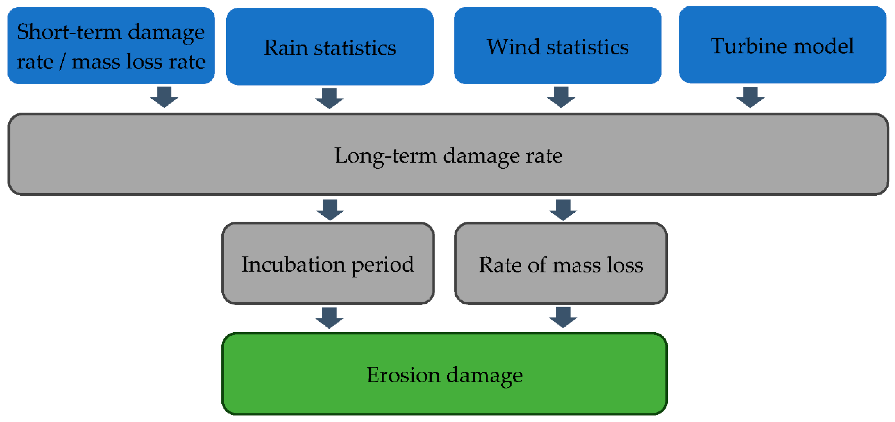
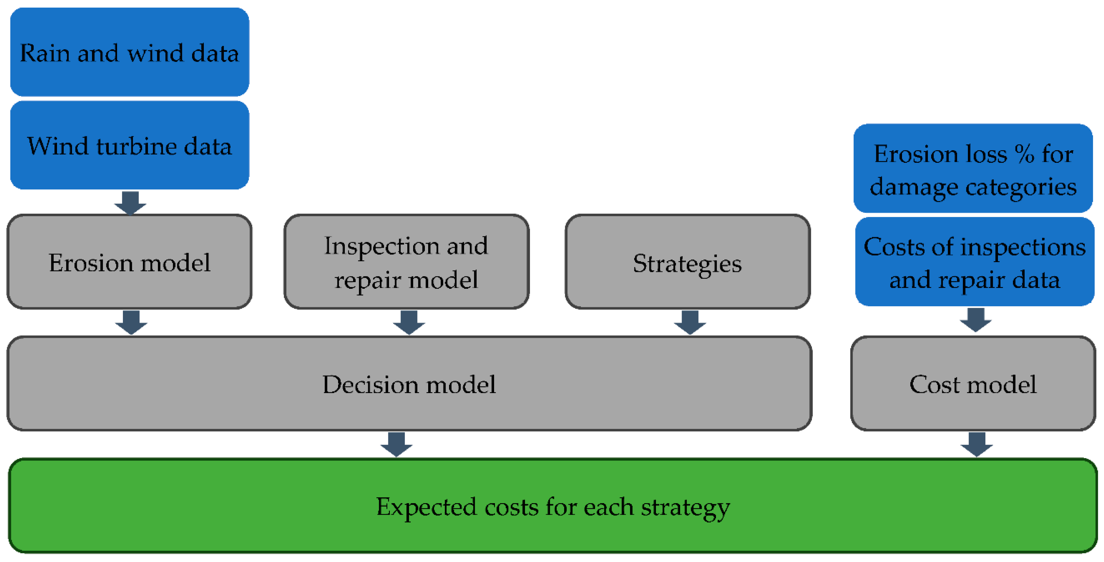
This section outlines the methodology employed in this study, focusing on the probabilistic modelling of erosion and the decision framework used to evaluate alternative maintenance strategies. The overall architecture of the implemented solution is illustrated in Figure 1.

2.1. Erosion Modelling

The erosion modelling in this work is based on a physics-based LEE model. In the model, the turbine blade’s leading-edge layer structure is simplified by assuming it consists of only two primary constituent layers: an outer protective coating and an inner structural reinforcement layer. This simplification is motivated by three key factors: first, it enables a concise erosion classification system, as presented in

Table 1. Definition of erosion categories (CAT) [46].

Erosion CAT	Description	Coating Mass Loss	Laminate Mass Loss
1	Light pitting of coating	<10%	0%
2	Small patches of missing coating	10–50%	0%
3	Large patches of missing coating	50–100%	<10%
4	Erosion of laminate (complete loss of coating)	100%	10–100%
5	Complete loss of laminate (laminate failure)	100%	100%

; second, it facilitates the classification of erosion in the field; and third, it enables the erosion modelling approach discussed in Section 2.1.1. The category is defined by erosion in the outer 5% of the blade length, where the erosion is expected to be most severe due to the high speed at the tip. Towards the root it will generally decline in severity.

2.1.1. Physics-Based Modelling of Leading Edge Erosion

To model the physical process of rain erosion initiation and progression for a specific site, the method developed by Verma et al. [40] is used, where the probability distribution of wind and rain statistics are integrated into the Springer model [29] to produce a long-term average damage rate to predict erosion initiation for a specific wind farm site and turbine. Assumptions of this model include the following: 1. the material acts linearly elastic; 2. erosion from solid particles such as sand and hail are neglected; 3. sequence effects in fatigue are neglected; and 4. the material architecture of a turbine blade’s leading edge is assumed to consist of only two main layers, an outer coating and inner structural reinforcement material. We have extended Verma et al.’s [40] method to include erosion of coated materials (instead of a single homogeneous material) and to predict mass loss rate in addition to damage initiation. A brief explanation and mathematical description of the site-specific damage initiation and progression model is presented below. An overview of the calculation procedure is shown in Figure 2.

The damage initiation phase is split into two models: a damage initiation model for the coating, and a damage initiation model for the substrate. Using Springers model for coated materials the dimensionless number of impacts until damage initiation, $n_i^{*}$, is calculated as:

$$n_i^{\mathrm{*}}=7.1\cdot {10}^{-6}{\left({\displaystyle \frac{S}{{\overline{\sigma }}_0}}{\displaystyle \frac{1}{1+2\overline{k}\left|{\psi }_{sc}\right|}}\right)}^{5.7}$$

(1)

where S is the erosive strength of the coating material, ${\overline{\sigma }}_0$ is pressure felt at the interface of the rain droplet and coating, $\overline{k}$ is the number of reflections that occur while the droplet is impacting the coating, and ${\psi }_{sc}$ is the relative impedance between the substrate and the coating. A similar process is used to calculate the dimensionless number of impacts until damage initiation of the substrate:

$$n_i^{\mathrm{*}}=7.1\cdot {10}^{-6}{\left({\displaystyle \frac{S}{P}}\right)}^{5.7}$$

(2)

The dimensionless number of impacts until damage initiation is then converted into number of impacts until failure per unit area with the following equation, where $d$ is the diameter of the rain droplet.

$$n_i={\displaystyle \frac{4}{\pi d^2}}{n}_i^{*}$$

(3)

Another key component to fatigue analysis is determining the rate of loading, in this case the rate of rain droplet impacts on the leading edge, $\dot{n}$. To calculate this Equation (4) is used, where q is the number of rain droplets per metre cubed, which is dependent on droplet diameter, wind speed $U_w$, and rain intensity I. $V_{imp}$ is the velocity at which the rain droplets impact the blade leading edge and is dependent on droplet diameter and wind speed. ${\beta }_d$ is the impingement efficiency and is dependent on the droplet diameter.

$$\dot{n}=q\cdot V_{imp}\cdot {\beta }_d$$

(4)

With both the impacts until failure and impact rate calculated, Palmgren–Miner’s rule can then be applied with Equation (5) to determine the “short-term damage rate” with units of ${time}^{-1}$. The short-term damage rate is computed for both coating and substrate materials.

$$D^{ST}={\displaystyle \frac{\dot{n}}{n_i}}$$

(5)

Once the short-term damage rate for both the coating and substrate can be determined, a long-term averaged damage rate for a specific site can be computed using Equation (6). The joint probability distribution of droplet size and rain intensity $f_{d,I}\left(I_i,d_j\right)$ is computed by multiplying the lognormal distribution of rain intensity with the two-parameter Weibull distribution of droplet size distribution (DSD). The parameters of DSD are defined conditional on the rain intensity by parameters $A,p,N$ and $q$. $f_{U_w}\left(U_{w_k}\right)$ is the two-parameter Weibull distribution of wind speed, and $P\left(I_i\right)$ is the probability of occurrence of rain at a given intensity for a specific site and is modelled as a step function.

$$D^{LT}=\sum _i^{\infty }\sum _j^{\infty }\sum _k^{\infty }{D}_{ijk}^{ST}\left(I_i,d_j,U_{w_k}\right)f_{d,I}\left(I_i,d_j\right)P\left(I_i\right)f_{U_w}\left(U_{w_k}\right)∆I∆d∆U_w$$

(6)

The long-term damage rate also has units of ${time}^{-1}$ and when $D^{LT}\cdot t\ge 1$, the coating or substrate has failed. See refs. [1,2,12,13] for additional information and insight into the derivation and inputs into Equations (1)–(6).

A model of damage progression, once damage has been initiated, is also needed for a risk-based maintenance strategy. To calculate this, the dimensionless mass loss rate relationship to the dimensionless number of impacts for both the coating and substrate taken from Springer [28,29] is used as shown in Equation (7).

$${\alpha }^{*}=0.023{\left({\displaystyle \frac{1}{n_i^{*}}}\right)}^{0.7}$$

(7)

The dimensionless mass loss rate is then converted to a short-term mass loss rate with Equation (8). The short-term mass loss rate, ${\alpha }^{ST}$has units of ${\displaystyle \frac{mass}{unitarea\cdot time}}$, and ${\rho }_l$ is the density of the rain droplet.

$${\alpha }^{ST}={\alpha }^{*}{\displaystyle \frac{\pi {\rho }_l{d}^3}{4}}(q{V}_{imp}{\beta }_d)$$

(8)

The long-term mass loss rate is then computed using a similar expression as was used to determine the long-term damage initiation rate in Equation (6) and can be seen in Equation (9).

$${\alpha }^{LT}=\sum _i^{\infty }\sum _j^{\infty }\sum _k^{\infty }{\alpha }_{ijk}^{ST}\left(I_i,d_j,U_{w_k}\right)f_{d,I}\left(I_i,d_j\right)P\left(I_i\right)f_{U_w}\left(U_{w_k}\right)∆I∆d∆U_w$$

(9)

Finally, the mass loss per unit area for a given time can be calculated with Equation (10), where $m$ has units of ${\displaystyle \frac{mass}{unitarea}}$.

$$m={\alpha }^{LT}(t_f-t_i)$$

(10)

A key assumption in this analysis is that the substrate is fatiguing towards initiation while the coating is still covering it. However, the substrate cannot begin to lose mass until the coating in the unit area being analyzed has eroded away completely. For the model to be applicable within a risk-based maintenance strategy, it must be transformed into a stochastic framework. Although the model incorporates probability distributions for weather data, the results are deterministic, as it consolidates the results into an average damage and mass loss rate. To transition to a stochastic approach, the Weibull parameters for droplet size and rain intensity, along with wind speed and the mean and standard deviation for rain intensity, are treated as time-variant stochastic variables characterized by normal distributions. These variables are re-evaluated annually within Monte Carlo simulations, allowing the recalibration of damage initiation and mass loss rates to reflect minor annual variations in weather conditions.

2.1.2. Probabilistic Bayesian Network Model

Evaluating the physics-based erosion model through Monte Carlo simulations is computationally intensive and inefficient for integration within a decision model. To enable efficient decision-making, the erosion process is instead represented using a Bayesian network formulation. However, constructing the conditional probability tables (CPTs) for the Bayesian network still requires numerous runs of the erosion model.

Importantly, the erosion model’s outputs of interest are limited to the statistical description of three key parameters: the annual erosion damage rate $D^{LT}$, the coating mass loss rate ${\alpha }^{LTC}$, and the laminate mass loss rate ${\alpha }^{LTL}$, as all environmental information is condensed into these parameters. These parameters effectively represent the influence of environmental conditions, making them suitable for a simplified probabilistic representation.

Since $D^{LT}$, ${\alpha }^{LTC}$, and ${\alpha }^{LTL}$ are not statistically independent, their interdependencies must be captured. From Equation (7), it is evident that $\ln \left({\alpha }^{*}\right)$ depends linearly on $\ln \left({\displaystyle \frac{1}{n_i^{*}}}\right)$, and from Equations (3), (5), and (8) it can be seen that $\ln \left({\alpha }^{ST}\right)$ also exhibits a linear relationship with $\ln \left(D^{ST}\right)$. A similar relationship is expected for the long-term parameters, albeit with added uncertainty.

In this study, $D^{LT}$ is modelled as a stochastic variable with a probability distribution fitted to values obtained from the erosion model. The parameters ${\alpha }^{LTC}$ and ${\alpha }^{LTL}$ are then modelled as stochastic variables conditioned on $D^{LT}$. Figure 3a presents a PDF-scaled histogram of $D^{LT}$ values generated by the erosion model along with a fitted generalized extreme value distribution. Figure 3b illustrates the linear relationship between $\ln \left({\alpha }^{LTC}\right)$, $\ln \left({\alpha }^{LTL}\right)$, and $\ln \left(D^{LT}\right)$, confirming the expected correlation. Linear regression is used to estimate the coefficients of this relationship, and a three-parameter Weibull distribution is fitted to the residuals. This approach yields a condensed probabilistic representation of the erosion model, enabling efficient integration into the Bayesian decision framework.

The erosion model described above incorporates physical uncertainties; however, model uncertainties must also be considered. To account for these, additional uncertainty factors are introduced into the calculation of the damage rate, which influences both the incubation period and the mass loss rates through the relationships previously described.

Model uncertainty comprises both time-variant and time-invariant components. The time-variant component is primarily associated with uncertainties in the load model—such as the exclusion of hail—which may vary in impact from year to year. In contrast, the time-invariant component is largely related to uncertainties in the resistance model and includes physical uncertainties in the model parameters.

To incorporate these uncertainties, the annual (long-term) damage rate is expressed as the following:

$$D^{LTX}=D^{LT}\cdot X_{load}\cdot X_{res}$$

(11)

where $X_{load}$ is the time-variant load model uncertainty and $X_{res}$ is the time-invariant resistance model uncertainty.

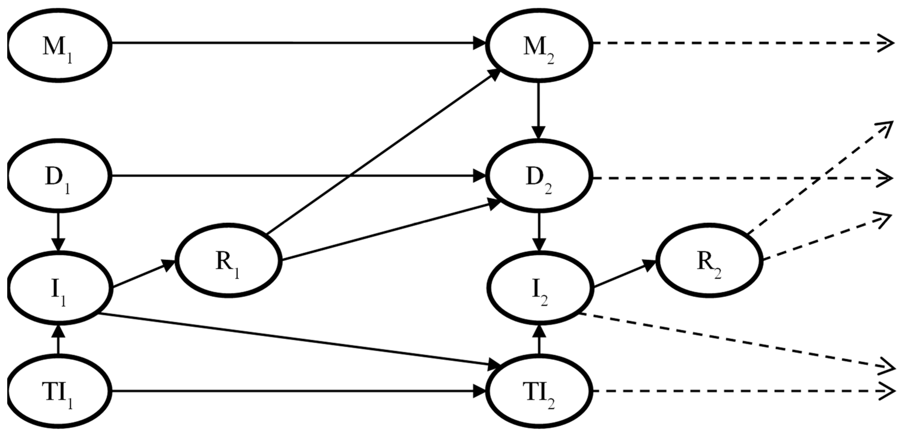
Figure 4 illustrates the structure of a simplified dynamic Bayesian network (DBN) degradation model. Each time slice consists of two nodes: D, representing damage, and M, representing the time-invariant model uncertainty, here corresponding to $X_{res}$.

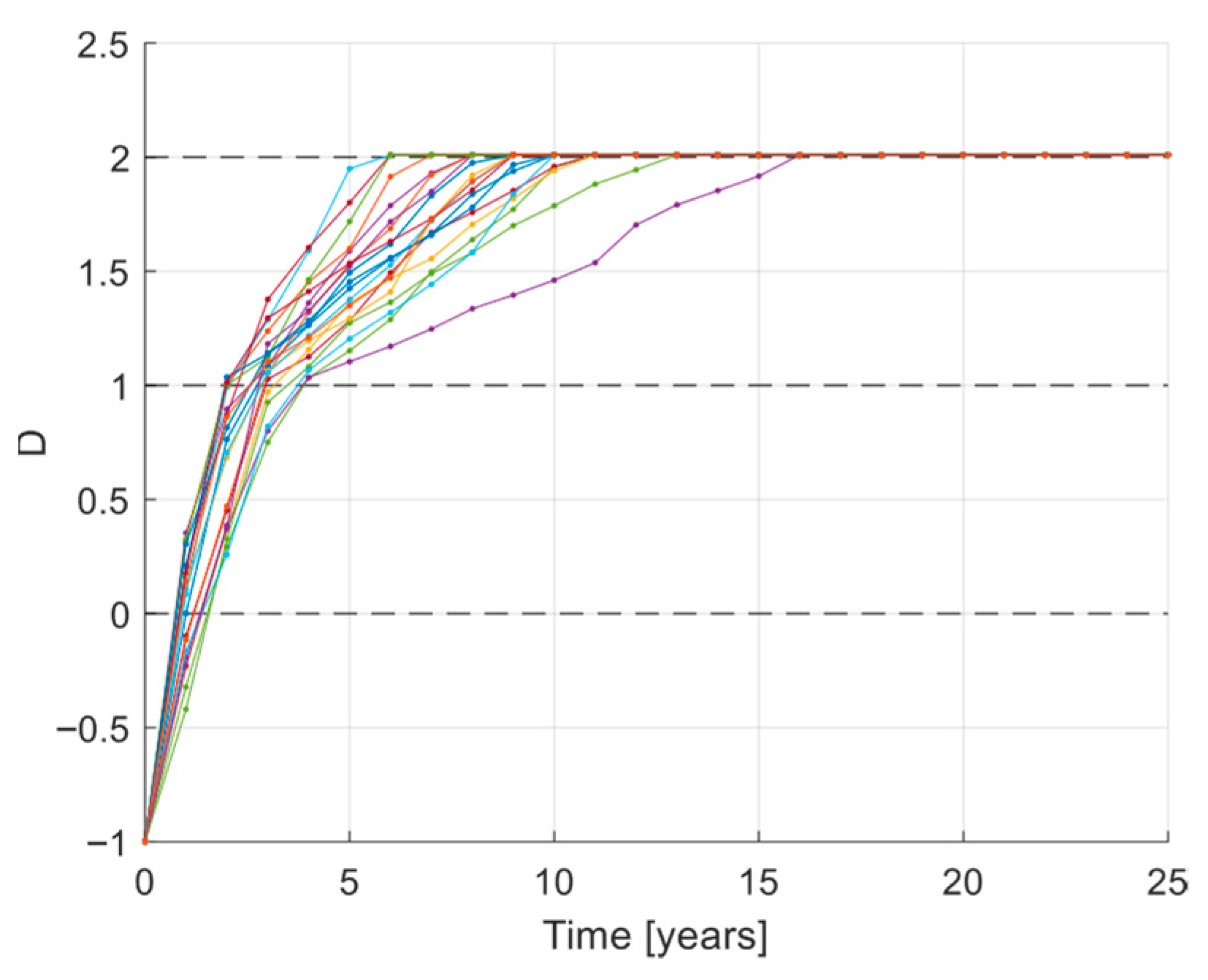
The erosion model consists of three distinct phases: the incubation period, the coating mass loss phase, and the laminate mass loss phase. Accurate representation of these phases—including correct incubation timing and mass loss behaviour—requires a DBN model with a sufficient number of states to capture the progression within each phase. For instance, modelling the incubation period with a single state would imply a geometric distribution for the transition time, as the probability of moving to the next phase would remain constant at each time step. Instead, a damage number is used to represent the progression of damage during the incubation period. The node $D$ is used to model the damage through all phases by defining relative intervals for each phase:

• $-1<D\le 0$: Incubation phase;
• $0<D\le 1$: Coating mass loss phase;
• $1<D\le 2$: Laminate mass loss phase.

With this definition of $D$, sampling from the condensed model with included model uncertainties leads to Figure 5.

The DBN erosion model is defined by the conditional probability table $P\left(D_i\right|D_{i-1},M_i)$ and by the tables for the initial damage state $P\left(D_0\right)$ and model uncertainty $P\left(M_0\right)$. The number of states for each node is selected using a convergence analysis, ensuring that the distribution for the predicted time to initiation, time to coating failure, and time to laminate failure correspond to the distributions obtained using Monte Carlo simulations. For the base model presented in Section 3, it was found sufficient to model $D$ by 151 states and $M$ by 10 states. As the erosion model explicitly models the incubation period, the initial damage state is always the first state, thus $P\left(D_0\right)$ is a vector with one in the first entry, while the rest are zeros. $P\left(M_0\right)$ is calculated directly from the lognormal distribution. $P\left(D_i\right|D_{i-1},M_i)$ is calculated using the condensed probabilistic model. For each combination of states for $D_{i-1}$ and $M_i$, $2.5\cdot {10}^5$ samples were drawn (by dividing both into 50 subintervals, and drawing 100 samples in each subinterval), and the condensed probabilistic model was used to calculate the damage state the following year $D_i.$ The distribution for $P\left(D_i\right|D_{i-1},M_i)$ was then established based on which states the samples ended in.

In total, the condensed model was called $4\cdot {10}^8$ times, resulting in a CPT calculation time of 200 s. Using the DBN model, the probabilistic progression of erosion over 20 years was calculated in 0.02 s, and in Figure 6 the time to initiation, time to coating failure, and time to laminate failure (hole in the blade) is shown. The figure also shows the results obtained using 1000 Monte Carlo simulations using the condensed model, which took 150 times longer. It is seen that the two models yield almost identical results. The physical model would take $3.5\cdot {10}^5$ times longer than the DBN model for 1000 simulations.

2.2. Decision-Making

This section introduces a novel heuristic approach for optimally scheduling inspections and repairs of deteriorating components. The deterioration, inspection, and repair processes are modelled probabilistically using Bayesian networks. In this study, erosion serves as the deterioration model, incorporating both time-variant and time-invariant uncertainties. A cost model captures expenses related to inspections, repairs, and aerodynamic performance loss. The objective is to identify a strategy that minimizes total lifetime costs by defining decision rules for inspection and repair timing based on observed damage.

To efficiently estimate expected lifetime costs, a discrete Bayesian network is developed, where decision rules are encoded in conditional probability tables. This enables exact inference of inspection and repair probabilities at each time step. A key innovation is the ability to vary the timing of subsequent inspections based on the most recent inspection outcome. Even when inspection intervals are fixed, the model allows for individualized schedules for blades repaired outside regular maintenance campaigns due to forced repairs of CAT 5 damage.

The methodology also supports adaptive strategies. Initially, the optimal strategy is based on prior deterioration and cost models. However, if observed damage progression deviates significantly from expectations, Bayesian updating is used to revise the deterioration model. The strategy is then re-optimized to reflect new information, and the expected benefit of adaptation is evaluated each time the strategy is updated. The updating of strategies can be performed whenever an inspection has been performed, or whenever it is practical to update strategies.

Bayesian Network Model

The core of the methodology is a discrete DBN with the structure as shown in Figure 7. The network consists of identical time slices, one for each time, each containing five discrete nodes, which may represent underlying continuous variables:

• $M_i$: time-invariant deterioration parameter, discretized into intervals.
• $D_i$: damage state, discretized into intervals.
• $I_i$: inspection outcome states for each possible outcome, including a dummy state for ‘no inspection’.
• $R_i$: repair decision, with states ‘repair’ and ‘no repair’.
• $T{I}_i$: time until the next inspection, functioning as a countdown between inspections and resetting based on the strategy. States range from 1 to the maximum inspection interval.

Deterioration is modelled by the conditional distribution $P\left(D_i\right|D_{i-1},M_i)$, the prior distribution for the model parameter $P\left(M_1\right)$, and the prior distribution for the initial damage state $P\left(D_1\right)$. The distribution $P\left(M_i\right|M_{i-1})$ is the identity matrix as M is time-invariant. The nodes D and M also have the repair node as a parent, as repairs affect the damage state and possibly the time-invariant model parameter. Appendix A provides further details on the implementation of repairs, inspections, decision strategies, inference algorithms, and adaptive strategy updates.

3. Case Study

The aim of the case study is to demonstrate how the framework can be applied to optimize decisions on when to inspect and repair blades for LEE and investigate how site conditions and other parameters affect optimal strategies.

Costs associated with LEE are primarily associated with energy loss due to aerodynamic performance impacts, repair costs, inspection, and lost production incurred during repair and inspection downtime.

3.1. Input

As a base case, the case study considers erosion of the NREL 5MW reference turbines on inland sites with IEC class II [47]. Through a parameter study, the influence of various parameters is investigated, and therefore input parameters are presented for IEC classes I, II, and III; cost models corresponding to onshore and offshore conditions; and rain models corresponding to inland and costal sites.

3.1.1. Erosion Model

Erosion is modelled using the approach presented in Section 2.1. The material parameters used in the erosion model are given in

Table 2. Material parameters based on [48,49,50].

Parameter	Coating	Substrate	Water
$\rho$$[\mathrm{k}\mathrm{g}/{\mathrm{m}}^3$] Density	1100	1900	1000
$E\left[\mathrm{P}\mathrm{a}\right]$ Modulus of elasticity	-	2.41 × 109
${\sigma }_{ult}\left[\mathrm{P}\mathrm{a}\right]$ Ultimate strength	37 × 106	67.3 × 106
$m$ [-] Wöhler exponent	16.92	7
$\nu$ [-] Poisson’s ratio	0.3	0.3
$c[\mathrm{m}/\mathrm{s}]$ Speed of sound	1900	2740	1480
$t\left[\mathrm{m}\right]$ Material thickness	0.0004572	0.0016

. The erosion model captures damage progression up to CAT5, which corresponds to through-thickness erosion (the entire blade shell thickness is eroded). In practice, erosion may continue to consume more of the blade, potentially compromising the structural integrity of the blade. The model assumes that once through-thickness damage occurs, it is detected by the monitoring system and triggers an unplanned inspection and subsequent repair—regardless of the applied maintenance strategy.

The rain conditions are represented by the distribution for the rain intensity and the conditional distribution of the droplet size, given rain intensity. We consider rain conditions corresponding to an inland site and a coastal site, based on sites De Bilt and De Kooy [40]. The inland site has a higher frequency of heavy rainfall and has generally smaller rain droplets. This means that, for the same rain intensity, there are more droplets at the inland site. For the same wind conditions, the inland site will therefore experience more erosion than the coastal site so the rain model for the inland site will be referred to as the high rain intensity model. Following [40], the rain intensity $I$ is modelled by a lognormal distribution with parameters ${\mu }_I$ and ${\sigma }_I$, and the droplet site distribution (DSD) is modelled by a two-parameter Weibull distribution with scale parameter $a=A\cdot I^p$ and shape parameter $n=N\cdot I^q$. All parameter values are given in

Table 3. Rain intensity and droplet size distribution (DSD) parameters [40].

Parameter	Inland (High Rain Intensity)	Coastal (Low Rain Intensity)	Standard Deviation
$\mathrm{Rain}\mathrm{intensity}{\mu }_I$	−0.1816	−0.1445	0.01
$\mathrm{Rain}\mathrm{intensity}{\sigma }_I$	0.8617	0.8275	0.01
$\mathrm{DSD}N$	4.5670	2.83	0.1
$\mathrm{DSD}q$	0.1404	−0.0953	0.01
$\mathrm{DSD}A$	0.4811	1.03	0.1
$\mathrm{DSD}p$	0.1186	0.138	0.01

.

The wind conditions are defined through the IEC classes, where classes I, II, and III have mean wind speeds of 10 m/s, 8.5 m/s, and 7.5 m/s, respectively. The 10 min mean wind speed is modelled by a two-parameter Weibull distribution with the shape parameter equal to two, and scale parameter calculated to achieve the desired mean value. To reflect uncertainties on wind conditions on sites, the uncertainties of the annual values are modelled using normal distributions with standard deviations equal to 0.05 and 1 for the shape and scale parameter, respectively.

The model uncertainty on the load, $X_{load}$, and resistance, $X_{res}$, are modelled by lognormal variables with mean equal to one and standard deviations 0.1 and 0.2, respectively.

3.1.2. Inspection Model

Exterior blade inspections are commonly carried out by drones equipped with cameras. Alternatively, they may be carried out by humans from the ground with high-zoom cameras but, because drone-based inspections are increasingly becoming industry standard, this work considered only drone inspections. Interior inspections are typically carried out irregularly, driven by a known issue or risk. Interior inspections are not considered as part of this work.

No inspection can identify all damage, and the likelihood of identifying a specific instance of damage decreases as the damage size decreases. Some inspection methods are well studied and have probability of detection curves (decreasing probability as the finding size decreases). The wind industry does not have well-vetted probability of detection curves for drone-based exterior inspections, so the authors of this paper utilized an average of expert opinion across eight experts who regularly inspect wind turbine blades or review inspections performed by others. The results of this exercise are shown in

Table 4. Likelihood of reporting a given damage category given the actual damage category.

Actual Erosion Category		Reported Erosion Category
	No Detection	CAT 1	CAT 2	CAT 3	CAT 4	CAT 5
CAT 1	75%	10%	9%	5%	1%	0%
CAT 2	30%	11%	28%	21%	7%	4%
CAT 3	20%	4%	16%	36%	20%	4%
CAT 4	5%	0%	14%	24%	43%	14%
CAT 5	0%	0%	5%	10%	40%	45%

.

3.1.3. Cost Model

The following cost components are input to the decision model and must be estimated for the sites under consideration:

• Lost production due to aerodynamic losses caused by LEE;
• Lost production due to downtime from LEE-related inspections or repair activities;
• Direct repair costs, including materials, labour, and associated support services;
• Direct inspection costs.

These cost parameters are defined for the example wind farms based on industry experience in the U.S. and are selected to represent typical onshore and offshore wind farm conditions. The specific values are provided in

Table 5. Input parameters used in the cost model based on industry experience in the US. Costs in US dollars per turbine.

Parameter	Onshore	Offshore
Inspection cost	$250	$400
Mobilization costs for repairs	$1000	$2444
Repair costs per day	$5000	$12,222
Repair duration (with 10 working hours per day)	CAT 1: 2 days	CAT 1: 3 days
	CAT 2: 3 days	CAT 2: 5 days
	CAT 3: 6 days	CAT 3: 9 days
	CAT 4: 7 days	CAT 4: 11 days
	CAT 5: 14 days	CAT 5: 21 days
Inspection duration	0.25 h	0.5 h
Energy price	$25 per MWh	$25 per MWh

.

LEE will negatively impact the blade’s aerodynamic performance. For the purposes of this case study, we have quantified energy loss due to aerodynamic performance impacts in terms of AEP loss because it can easily be translated to lost revenue. Based on an aggregation of papers referenced in Section 1.2, we developed the relationship between LEE severity category and AEP loss. The AEP loss is dependent on the site’s wind class because LEE only impacts power capture below rated power, and a wind turbine will spend less time below rated power in lower wind environments. The resulting AEP losses have therefore been calculated based on the power curve and mean wind speed distribution.

Table 6. Capacity factor and AEP loss as a function of LEE severity and annual average wind speed (v_avg).

Parameter	Wind Class
	I (vavg = 10 m/s)	II (vavg = 8.5 m/s)	III (vavg = 7.5 m/s)
Annual average capacity factor	56.7%	46.3%	37.9%
Capacity factor during repair	13.9%	15.8%	16.4%
AEP loss CAT 1	0.0%	0.0%	0.0%
AEP loss CAT 2	0.4%	0.6%	0.7%
AEP loss CAT 3	0.8%	1.1%	1.3%
AEP loss CAT 4	1.6%	1.9%	2.2%
AEP loss CAT 5	2.0%	2.7%	2.9%

shows the AEP loss for each IEC wind class as well as the annual average capacity factor and the capacity factor during repair and inspection periods, assuming that these are performed in low wind periods.

The parameters in Table 5 and Table 6 were used to calculate the direct inputs to the decision model, listed in

Table 7. Decision model inputs for the onshore cost model.

	Direct Costs ($)	Revenue Loss From Downtime ($)			Revenue Loss From Aerodynamic Losses ($/year)
		Class I	Class II	Class III	Class I	Class II	Class III
Inspection	$250	$4	$5	$5	-	-	-
CAT 1	$11,000	$348	$395	$410	$0	$0	$0
CAT 2	$16,000	$522	$592	$616	$2485	$3041	$2901
CAT 3	$31,000	$1044	$1184	$1231	$4970	$5576	$5388
CAT 4	$36,000	$1218	$1382	$1437	$9941	$9631	$9118
CAT 5	$71,000	$2436	$2763	$2873	$12,426	$13,686	$12,019

for the onshore site.

3.2. Results of Decision Model

Initially, the decision model was run for the IEC class II site with the inland rain model (high rain intensity) and onshore cost model. The inspection strategies modelled had constant inspection intervals of 1, 2, 3, 4, 5, 7, 9, and 13 years; a strategy with no planned inspections was also modelled. The inspection intervals excluded from this list were not modelled because they will never be optimal; for example, inspection intervals of both 5 and 6 years will lead to four inspections during the lifetime of 25 years, but the inspections are more optimally distributed over time with the 5-year interval. It was assumed that repairs would be made when LEE damage CAT 1 to CAT 4 was detected (referred to as the “repair threshold”). Repairs were assumed to be performed whenever the erosion category reaches CAT 5 or when erosion exceeding the repair threshold is detected at an inspection. In all, 33 strategies were modelled. The numbering of strategies is shown in

Table 8. Numbering of strategies.

Inspection Interval Repair Threshold	1	2	3	4	5	7	9	13	No Inspections
CAT 1	1	2	3	4	5	6	7	8	-
CAT 2	9	10	11	12	13	14	15	16	-
CAT 3	17	18	19	20	21	22	23	24	-
CAT 4	25	26	27	28	29	30	31	32	-
CAT 5	-	-	-	-	-	-	-	-	33

for use in later figures.

In Figure 8a, the expected number of lifetime inspections and repairs of each type is shown for each of the strategies. The results show that increasing the inspection intervals leads to fewer repairs as well as fewer inspections, and at the point of repair, blades will have a higher damage category. Increasing the repair threshold also leads to a decrease in the number of repairs, and an increase in damage category at the point of blade repair. Due to the inspection uncertainty, a portion of the repairs are below the repair threshold, because they were (mis)categorized as being of a higher category than they should have been.

In Figure 8b, the total expected lifetime costs (referred to as expected costs in the following) associated with each of the strategies are shown associated with LEE AEP loss, inspections, and repairs of each category. For short inspection intervals and low repair thresholds, the expected costs are dominated by repairs of lower categories (CAT 1–3), whereas for increased inspection intervals and repair thresholds, the costs are increasingly dominated by repairs of higher categories (CAT 4–5) and LEE AEP loss. The lowest cost strategies are no. 5 and 13 (5-year interval and repair threshold equal to CAT 1 and CAT 2) with almost identical costs, and no. 6 and 14 (7-year interval and repair threshold equal to CAT 1 and CAT 2) have only slightly higher costs. The model was also run for strategies where the time to the next inspection would depend on the inspection outcome. However, none of these strategies outperformed the strategies with constant inspection intervals. An exception to this is presented in the parameter study in Section 3.3.7.

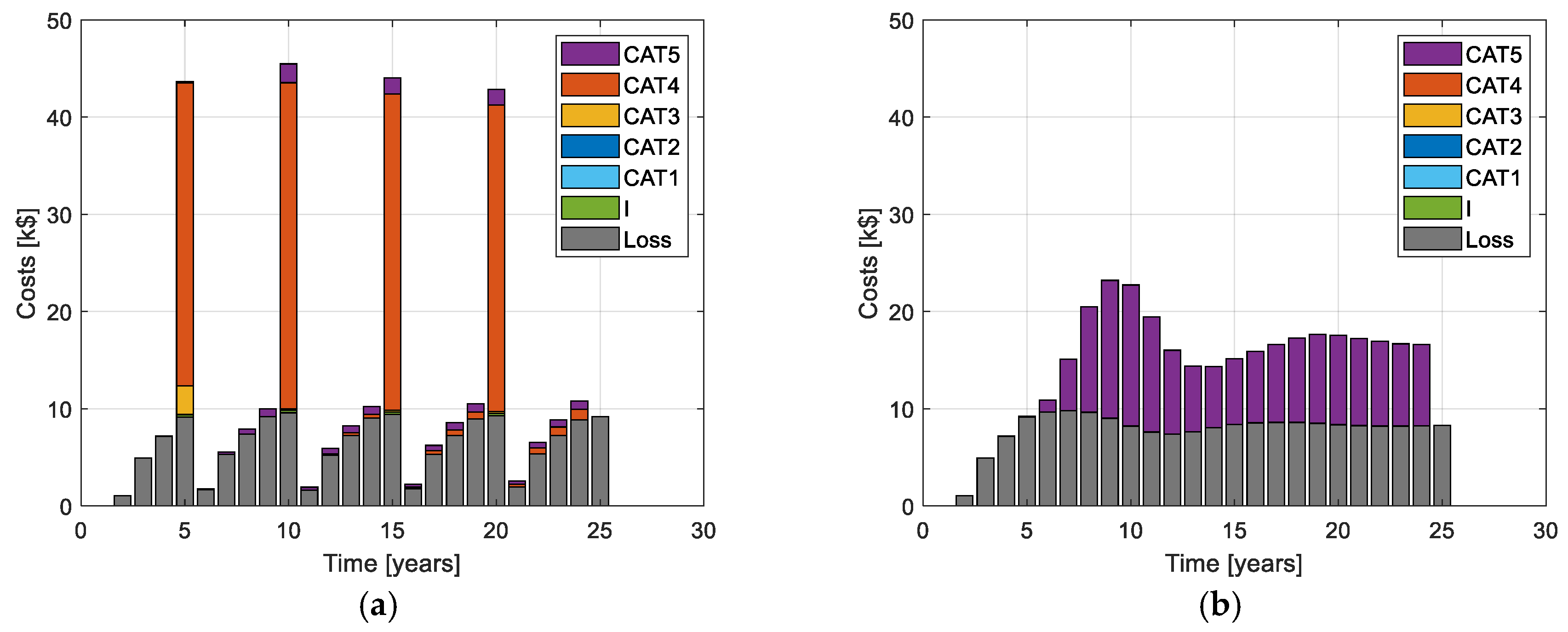
Figure 9 shows the distribution of costs over the 25-year lifetime for the best strategy (no. 13) and for the worst strategy (no. 33). For the best strategy, large repair costs are seen every fifth year, when inspections are primarily performed. The repairs lead to a drop in the LEE AEP loss, which increases initially and between inspections. Between the main inspection campaigns, some repairs are also made due to blades reaching CAT 5 between inspections, and because the inspection schedule for these blades will follow the time since the last repair, and therefore not follow the main inspection campaigns. For the worst strategy, an initial increase in LEE AEP loss is seen, followed by an increase in costs of CAT5 repairs. The costs then decrease again and reach a quite stable level for the last ten years of the lifetime.

3.3. Parameter Study

In this section, the effect of financial discounting, model uncertainty, LEE AEP loss percentage, IEC wind class, rain model, inspection model, and cost model are investigated.

3.3.1. Discounting

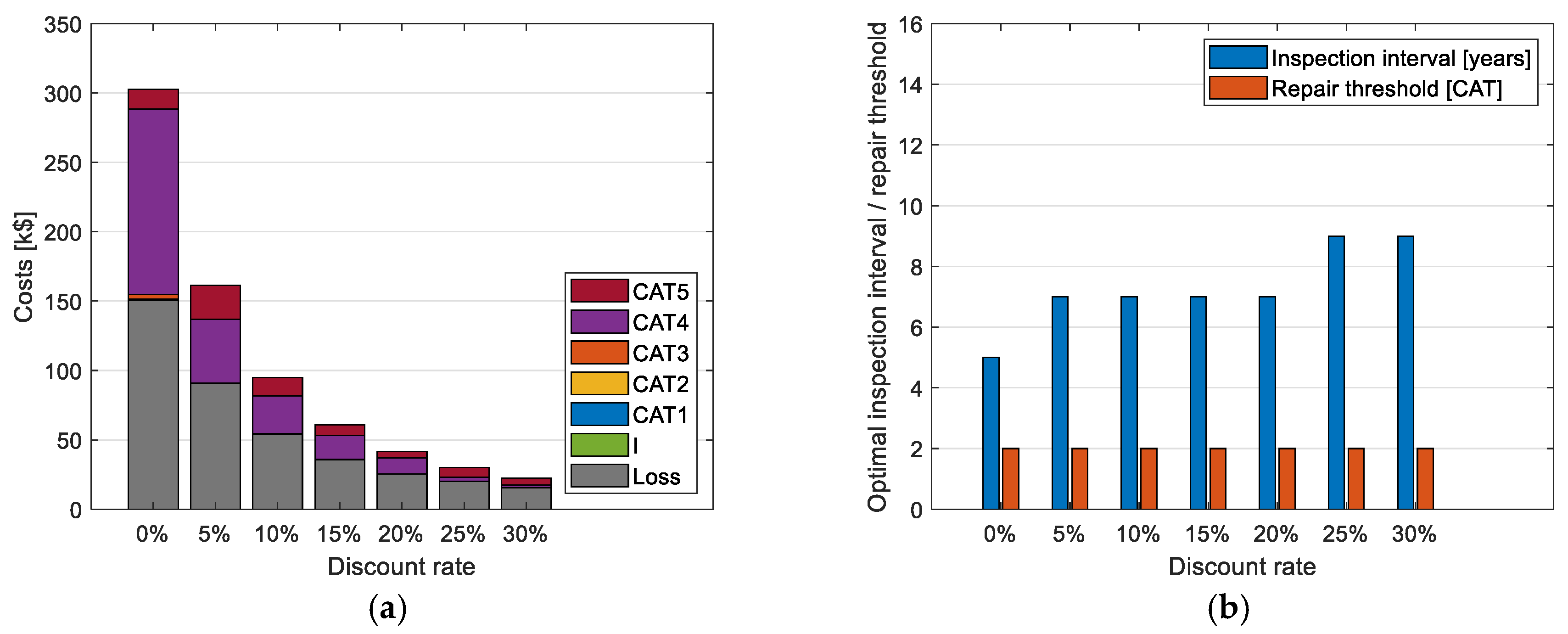
The initial calculations were performed without including a discount rate. Figure 10 shows the effect of the discount rate on which strategy is optimal and on the expected present value of the costs for the optimal strategy. The inclusion of a discount rate obviously leads to a decrease in the expected present value of the costs. However, it also leads to a change in the optimal strategy as the optimal inspection interval increases from 5 to 7 years for discount rates of 5–20% and to 9 years for discount rates of 25–30%. As seen in Figure 8b, the costs for these strategies (no. 13–15) were close to each other when no discount rate was included. As shown in Figure 11, the inclusion of a discount rate of 10% leads to a relative reduction in the expected present value of the costs for the strategies with longer inspection intervals compared to the shorter. This tips the balance such that another strategy is better. The reason is that longer inspection intervals mean the expenses are pushed into the future, which is favourable for the present value of the costs.

3.3.2. Model Uncertainty

Initially, the time-invariant model uncertainty coefficient of variation (COV) on the resistance $X_{res}$ was assumed to be 20%. Figure 12 shows the effect of the COV on the optimal strategy and the associated expected costs. It is seen that a decrease from 20% to 10% in model uncertainty COV increases the optimal inspection interval from 5 to 7 years and slightly decreases the costs, whereas an increase model uncertainty COV does not change the optimal strategy and only very slightly changes the costs.

3.3.3. LEE AEP Loss

As described in Section 3.1.3, the LEE AEP loss percentages given in Table 6 are uncertain. Figure 13 shows how the optimal strategy and expected costs are affected by varying the LEE AEP loss percentages in Table 6 by multiplication factors ranging from 0 to 2.5. It is seen that increased LEE AEP loss (factors larger than one) leads to a reduced repair threshold, and for factors 2 and 2.5, the optimal inspection interval is reduced to 1 year. This causes the expected costs of repairs of CAT 1–3 to dominate the costs, and the costs of LEE AEP loss decrease. If the LEE AEP loss percentages are multiplied by a factor smaller than one, the optimal inspection interval is 7 years because the benefit of more frequent inspections is reduced.

3.3.4. IEC Classes and Rain Distribution

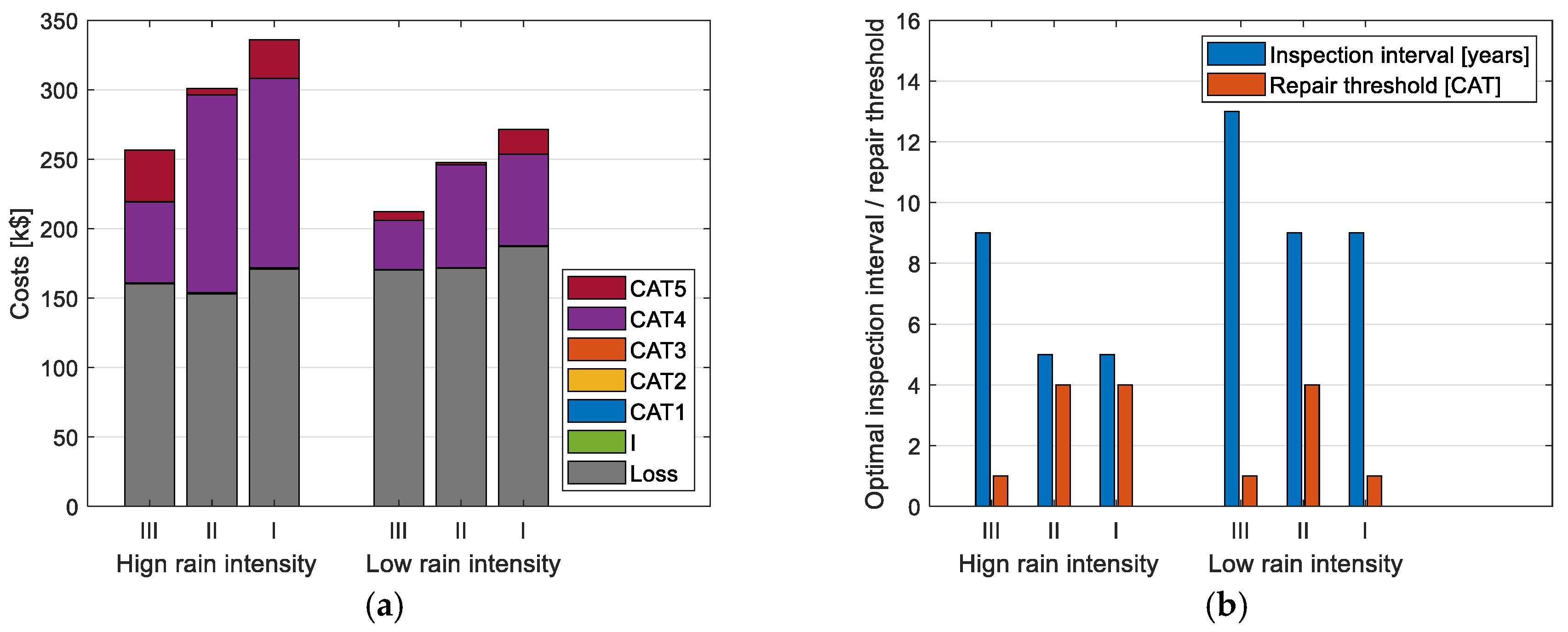
So far, the results have been shown for an IEC class II site with an inland rain model (high rain intensity). Figure 14 shows the optimal strategy and expected costs for sites with IEC class III, II, and I wind conditions (mean wind speeds 7.5, 8.5, and 10 m/s) and with high and low rain intensity models (inland and coastal rain models). As expected, higher wind speed and higher rain intensity both lead to increased expected costs and to smaller optimal inspection intervals.

3.3.5. Inspection Model

The inspection model presented in Table 4 was based on assumptions about the likelihood of reporting a given damage category given the actual damage category. To assess the impact of the high uncertainties related to this, the model was also run with a perfect inspection model, where the reported damage category is always equal to the actual damage category. Figure 15 shows the optimal strategies and the expected costs for the same six sites as in Figure 14 but using a perfect inspection model. It is seen that the costs are only slightly reduced when using a perfect inspection model. Only for one site, the IEC class III site with high rain intensity, is the optimal inspection interval changed. For some of the other sites, the optimal repair threshold is increased. However, examination of the top five strategies for each site revealed that, for the optimal inspection interval, the expected costs have little dependence on the repair threshold (less than 0.5% difference).

3.3.6. Offshore Cost Model

In the results shown so far, inspection and repair costs have been based on onshore sites. For offshore wind farms, these costs will generally be larger (as given in Table 5). Figure 16 shows the optimal strategies and expected costs for the six sites, when the offshore cost model is used. Generally, the expected costs are indeed larger than for the onshore cost model, and for three of the sites the optimal inspection interval is increased, as repairs are less feasible due to the increased costs.

3.3.7. Increased CAT 5 Repair Costs

In all results shown so far, the optimal inspection intervals have been constant, i.e., regardless of the inspection outcome, the time until the next inspection is constant over the lifetime. To investigate whether it would, in some cases, be optimal to use variable inspection intervals, various cost models were tested. It was found that if the costs of CAT 5 repairs were significantly increased, variable inspection intervals would be beneficial. If the CAT 5 repair costs were increased by a factor of six, the optimal strategy would be one with a variable inspection interval as shown in

Table 9. Optimal strategy if CAT 5 repair costs are increased by a factor of six.

	Initial and Following Repairs	CAT 1	CAT 2	CAT 3	CAT 4	CAT 5
Time to next inspection	2 years	2 years	1 years	Repair	Repair	Repair

.

3.4. Results of Adaptive Decision Model

In the results shown up until now, it is assumed that the same strategy is used throughout the lifetime. If, however, the model uncertainty on the resistance model is high, this might not be ideal as it means that the erosion rate will be highly uncertain. In Section 3.3.2 it was seen that the size of the model uncertainty did not have a large influence on the expected costs and on the optimal strategy. However, if the model uncertainty is large, it means that erosion could progress significantly faster or slower than expected, and the outcomes of the first inspections can give an indication of this. To address this, Bayesian updating can be used to update the decision model, and the decision model can be re-run for the remaining lifetime. This will be illustrated through an example. In this model, the resistance model uncertainty COV is increased to 100% to reflect a large level of uncertainty. It is assumed that the initial strategy is to inspect every five years, and to repair it if CAT 2 is reached. It is assumed that the inspections after five and ten years both give the same outcome, because repairs are made for outcomes equal to CAT 2 or higher. Figure 17 shows the optimal strategy and the expected costs for the remaining lifetime for inspection outcomes ranging from “no erosion detected” to CAT 5. It is seen that the expected costs in the remaining lifetime increase with the severity of the outcome. Further, if nothing is detected in both inspections, the inspection interval should be reduced to 3 years, and if the inspections both show CAT 5 erosion, the interval should be reduced to 4 years. For inspection outcomes up to CAT 3 it is beneficial to decrease the repair threshold to CAT 1. It is counterintuitive that inspections with no detection of erosion lead to a reduction in the inspection interval. The reason can be found in the large inspection model uncertainty. Although not detected, it is still likely that some degree of erosion is present, which will lead to LEE AEP loss. Therefore, it is beneficial to have an inspection after three years. The uncertainties related to the inspection model can also explain that the repair threshold should be reduced when erosion of the low categories is detected. Figure 18 shows the expected cost savings from changing from the original strategy to the optimal strategy after updating. It is seen that for CAT 1, the savings are estimated at 11.6%, whereas the savings for ‘no detection’ and CAT 5 are only 3.2% and 1.5%, and for CAT 2–4 savings are negligible.

4. Discussion and Conclusions

This section discusses the methodology, the results, and concludes the study. The methodology consists of four key components: the erosion model, the inspection and repair model, the cost model, and the decision model. Each component is critically examined below.

4.1. Erosion Model

The erosion model is based on a physics-driven analytical framework derived from the Springer model. While the base model has been validated in other contexts, the extension used here—which includes both coating degradation and mass loss—has not been independently validated. Wind farm operators with access to relevant data from wind farms could use their data to update model parameters and quantify uncertainties, but for the present study, validation of the erosion model for a specific site was beyond the scope. To account for this, a large model uncertainty was considered. However, this uncertainty had limited impact on the results. Instead, potential model bias appeared more influential, as evidenced by variations in optimal strategies under different rain and wind conditions, which gives an effect similar to model bias.

To address this, adaptive strategies were implemented, allowing the model to be updated based on observed data. In the example presented, the benefit of such updates was limited, though broader datasets from multiple turbines could enhance this effect.

A further limitation is that erosion categorization is based solely on blade tip erosion, ignoring the full distribution along the blade. A more sophisticated model could improve accuracy but would complicate the decision-making process due to a less direct relationship between erosion depth, category, repair cost, and performance loss.

To enable the construction of a Bayesian network, a simplified statistical erosion model was developed to reduce computational demands. This simplification introduces a loss of fidelity and weakens the direct link between environmental conditions and damage rates. Updating these variables would require recalculating the conditional probability distributions. However, explicitly including them in the Bayesian network would significantly increase both the model’s complexity and computation time. A potential improvement would be to model uncertainties in the coating and mass loss phases separately, as they may not be fully correlated. Future work should aim to facilitate model updates using operational, environmental, and inspection data, while maintaining computational efficiency.

4.2. Inspection and Repair Model

The inspection model incorporates significant uncertainties in both detection probability and damage classification accuracy. Surprisingly, these uncertainties had minimal impact on overall costs, as the use of a perfect inspection model only gave minor improvements. The optimal strategy compensates by lowering the repair threshold and extending inspection intervals, thereby reducing the frequency of repairs. For instance, a strategy may recommend repairing at CAT 1, yet due to a five-year inspection interval, repairs often occur at CAT 4 or 5.

The inspection uncertainty was not included when the erosion reached CAT 5 as it was assumed to be self-announcing. This assumption was found necessary to compensate for the lack of modelling of damage beyond CAT 5, as the model would underpredict the costs associated with continued operation without repair beyond CAT 5.

Repairs were assumed to be perfect—an optimistic simplification. In reality, repair modelling is complex, especially given the variety of erosion protection systems in use. While catastrophic blade failure due to extreme erosion is conceivable, operational experience suggests that repairs are typically performed well before such events occur. Therefore, this scenario was excluded from the model.

4.3. Cost Model

The cost model was established based on industry experience in the U.S., but the numbers would vary across wind farms and would be known with higher certainty by operators of specific wind farms. When applying the model for a specific wind farm, the specific cost numbers should be used. The prediction of the erosion production loss is more difficult, and it was found to be an important parameter, affecting the optimal strategy. In the present study it was based on erosion category, but it could also be modelled by a continuous relation with the extent of damage.

4.4. Decision Model

Heuristic strategies were employed to reflect current industry practices. However, more advanced optimization techniques could yield better and more adaptable decisions. As artificial intelligence becomes more integrated into operations, such methods may gain traction—provided their logic is transparent.

The decision model allowed inspection intervals to vary based on detected erosion category. Nonetheless, constant intervals were generally found to be optimal. These intervals were age-based rather than time-based, meaning each turbine followed a unique schedule post-repair. Non-constant intervals only proved beneficial when delaying repairs until just before CAT 5 yielded significant cost savings.

With the applied cost model, the expected costs across strategies were of the same order of magnitude, with a ~25% difference between the best and worst strategies. While this represents a meaningful saving, it also suggests that the model is reasonably balanced. More frequent inspections and lower repair thresholds lead to more, but less severe, repairs and reduced AEP loss. However, these effects tend to counteract each other, resulting in only minor changes to the total expected costs.

The present study focuses exclusively on decision-making related to leading edge erosion. However, the developed decision model is adaptable and can be applied to other failure modes, provided that appropriate degradation models are available. By formulating a unified cost model that incorporates shared costs across failure modes—such as inspection and mobilization expenses—the framework can be extended to encompass all relevant types of failures.

4.5. Conclusions

This study explored the requirements, methodologies, and limitations of implementing a decision support system for erosion management. The learnings are broadly applicable to other decision-making scenarios and illustrate the potential extent of data preparation, model development, and design trade-off considerations underpinning digitalization initiatives. The optimal strategy was found to depend on several factors, including discount rate, rain intensity and droplet size distribution, wind conditions, repair costs, and AEP loss. Therefore, project-specific data should be used. Future developments should focus on enabling continuous model updates using relevant data and incorporating AI-based optimization techniques that leverage all available information.

References

1. Dimitrov, N. Risk-based approach for rational categorization of damage observations from wind turbine blade inspections. J. Phys. Conf. Ser. 2018, 1037, 042021. [Google Scholar] [CrossRef]
2. Faber, M.H. Risk-based inspection: The framework. Struct. Eng. Int. J. Int. Assoc. Bridge Struct. Eng. (IABSE) 2002, 12, 186–194. [Google Scholar] [CrossRef]
3. Raiffa, H.; Schlaifer, R. Applied Statistical Decision Theory; Harvard University: Cambridge, MA, USA, 1961. [Google Scholar]
4. Straub, D.; Faber, M.H. Computational aspects of risk-based inspection planning. Comput.-Aided Civ. Infrastruct. Eng. 2006, 21, 179–192. [Google Scholar] [CrossRef]
5. Moan, T. Reliability-based management of inspection, maintenance and repair of offshore structures. Struct. Infrastruct. Eng. 2005, 1, 33–62. [Google Scholar] [CrossRef]
6. Robelin, C.-A.; Madanat, S.M. History-Dependent Bridge Deck Maintenance and Replacement Optimization with Markov Decision Processes. J. Infrastruct. Syst. 2007, 13, 195–201. [Google Scholar] [CrossRef]
7. Morato, P.G.; Mai, Q.A.; Rigo, P.; Nielsen, J.S. Point-based POMDP risk based inspection of offshore wind substructures. In Proceedings of the IALCCE 2018: The Sixth International Symposium on Life-Cycle Civil Engineering, Ghent, Belgium, 28–31 October 2018; pp. 3069–3076. [Google Scholar]
8. Nielsen, J.S.; Tcherniak, D.; Ulriksen, M.D. A Case Study on Risk-Based Maintenance of Wind Turbine Blades with Structural Health Monitoring. Struct. Infrastruct. Eng. 2020, 17, 302–318. [Google Scholar] [CrossRef]
9. Faber, M.H.; Sørensen, J.D.; Tychsen, J.; Straub, D. Field implementation of RBI for jacket structures. J. Offshore Mech. Arct. Eng. 2005, 127, 220–226. [Google Scholar] [CrossRef]
10. Lotsberg, I.; Sigurdsson, G.; Fjeldstad, A.; Moan, T. Probabilistic methods for planning of inspection for fatigue cracks in offshore structures. Mar. Struct. 2016, 46, 167–192. [Google Scholar] [CrossRef]
11. Straub, D. Stochastic modeling of deterioration processes through dynamic bayesian networks. J. Eng. Mech. 2009, 135, 1089–1099. [Google Scholar] [CrossRef]
12. Friis-Hansen, A. Bayesian Networks as a Decision Support Tool in Marine Application; Technical University of Denmark: Copenhagen, Denmark, 2000. [Google Scholar]
13. Nielsen, J.J.; Sørensen, J.D. Risk-based operation and maintenance of offshore wind turbines using Bayesian networks. In Applications of Statistics and Probability in Civil Engineering, Proceedings of the 11th International Conference on Applications of Statistics and Probability in Civil Engineering, ETH Zurich, Switzerland, 1–4 August 2011; CRC Press: Boca Raton, FL, USA, 2011. [Google Scholar]
14. Nielsen, J.S.; Sørensen, J.D. Computational framework for risk-based planning of inspections, maintenance and condition monitoring using discrete Bayesian networks. Struct. Infrastruct. Eng. 2018, 14, 1082–1094. [Google Scholar] [CrossRef]
15. Tien, I.; Der Kiureghian, A. Reliability Assessment of Critical Infrastructure Using Bayesian Networks. J. Infrastruct. Syst. 2017, 23, 04017025. [Google Scholar] [CrossRef]
16. Luque, J.; Straub, D. Reliability analysis and updating of deteriorating systems with dynamic Bayesian networks. Struct. Saf. 2016, 62, 34–46. [Google Scholar] [CrossRef]
17. Luque, J.; Straub, D. Risk-based optimal inspection strategies for structural systems using dynamic Bayesian networks. Struct. Saf. 2019, 76, 68–80. [Google Scholar] [CrossRef]
18. Bismut, E.; Straub, D. Optimal adaptive inspection and maintenance planning for deteriorating structural systems. Reliab. Eng. Syst. Saf. 2021, 215, 107891. [Google Scholar] [CrossRef]
19. Papakonstantinou, K.G.; Shinozuka, M. Planning structural inspection and maintenance policies via dynamic programming and Markov processes. Part II: POMDP implementation. Reliab. Eng. Syst. Saf. 2014, 130, 214–224. [Google Scholar] [CrossRef]
20. Corotis, R.B.; Ellis, J.H.; Jiang, M. Modeling of risk-based inspection, maintenance and-life cycle cost with partially observable Markov decision processes. Struct. Infrastruct. Eng. 2005, 1, 75–84. [Google Scholar] [CrossRef]
21. Kurniawati, H.; Hsu, D.; Lee, W.S. SARSOP: Efficient Point-Based POMDP Planning by Approximating Optimally Reachable Belief Spaces. In Robotics: Science and Systems IV; The MIT Press: Cambridge, MA, USA, 2008. [Google Scholar] [CrossRef]
22. Nielsen, J.S.; Sørensen, J.D. Risk-based decision making for deterioration processes using POMDP. In Proceedings of the 12th International Conference on Applications of Statistics and Probability in Civil Engineering, ICASP 2015, Vancouver, BC, Canada, 12–15 July 2015; University of British Columbia: Kelowna, BC, Canada, 2015. [Google Scholar]
23. Morato, P.G.; Papakonstantinou, K.G.; Andriotis, C.P.; Nielsen, J.S.; Rigo, P. Optimal Inspection and Maintenance Planning for Deteriorating Structural Components through Dynamic Bayesian Networks and Markov Decision Processes. Struct. Saf. 2022, 102140. [Google Scholar] [CrossRef]
24. Andriotis, C.P.; Papakonstantinou, K.G. Managing engineering systems with large state and action spaces through deep reinforcement learning. Reliab. Eng. Syst. Saf. 2019, 191, 106483. [Google Scholar] [CrossRef]
25. Andriotis, C.P.; Papakonstantinou, K.G. Deep reinforcement learning driven inspection and maintenance planning under incomplete information and constraints. Reliab. Eng. Syst. Saf. 2021, 212, 107551. [Google Scholar] [CrossRef]
26. Nielsen, J.S. Value of information of structural health monitoring with temporally dependent observations. Struct Health Monit 2022, 21, 165–184. [Google Scholar] [CrossRef]
27. Bismut, E.; Straub, D. A unifying review of NDE models towards optimal decision support. Struct. Saf. 2022, 97, 102213. [Google Scholar] [CrossRef]
28. Springer, G.S.; Yang, C.I. Model for the rain erosion of fiber reinforced composites. AIAA J. 1975, 13, 877–883. [Google Scholar] [CrossRef]
29. Springer, G.S.; Yang, C.I.; Larsen, P.S. Analysis of Rain Erosion of Coated Materials. J. Compos. Mater. 1974, 8, 229–252. [Google Scholar] [CrossRef]
30. Bech, J.I.; Hasager, C.B.; Bak, C. Extending the life of wind turbine blade leading edges by reducing the tip speed during extreme precipitation events. Wind. Energy Sci. 2018, 3, 729–748. [Google Scholar] [CrossRef]
31. Miner, M.A. Cumulative Damage in Fatigue. J. Appl. Mech. 1945, 12, A159–A164. [Google Scholar] [CrossRef]
32. Ansari, Q.M.; Sánchez, F.; Mishnaevsky, L.; Young, T.M. Evaluation of offshore wind turbine blades coating thickness effect on leading edge protection system subject to rain erosion. Renew Energy 2024, 226, 120378. [Google Scholar] [CrossRef]
33. Kuthe, N.; Mahajan, P.; Ahmad, S.; Mishnaevsky, L. Engineered anti-erosion coating for wind turbine blade protection: Computational analysis. Mater. Today Commun. 2022, 31, 103362. [Google Scholar] [CrossRef]
34. Doagou-Rad, S.; Mishnaevsky, L. Rain erosion of wind turbine blades: Computational analysis of parameters controlling the surface degradation. Meccanica 2020, 55, 725–743. [Google Scholar] [CrossRef]
35. Tempelis, A.; Mishnaevsky, L. Erosion modelling on reconstructed rough surfaces of wind turbine blades. Wind. Energy 2023, 26, 1017–1026. [Google Scholar] [CrossRef]
36. Verma, A.S.; Castro, S.G.P.; Jiang, Z.; Teuwen, J.J.E. Numerical investigation of rain droplet impact on offshore wind turbine blades under different rainfall conditions: A parametric study. Compos. Struct. 2020, 241, 112096. [Google Scholar] [CrossRef]
37. Visbech, J.; Göçmen, T.; Hasager, C.B.; Shkalov, H.; Handberg, M.; Nielsen, K.P. Introducing a data-driven approach to predict site-specific leading-edge erosion from mesoscale weather simulations. Wind. Energy Sci. 2023, 8, 173–191. [Google Scholar] [CrossRef]
38. Herring, R.; Domenech, L.; Renau, J.; Šakalytė, A.; Ward, C.; Dyer, K.; Sánchez, F. Assessment of a Wind Turbine Blade Erosion Lifetime Prediction Model with Industrial Protection Materials and Testing Methods. Coatings 2021, 11, 767. [Google Scholar] [CrossRef]
39. Eisenberg, D.; Laustsen, S.; Stege, J. Wind turbine blade coating leading edge rain erosion model: Development and validation. Wind. Energy 2018, 21, 942–951. [Google Scholar] [CrossRef]
40. Verma, A.S.; Jiang, Z.; Caboni, M.; Verhoef, H.; van der Mijle Meijer, H.; Castro, S.G.; Teuwen, J.J. A probabilistic rainfall model to estimate the leading-edge lifetime of wind turbine blade coating system. Renew Energy 2021, 178, 1435–1455. [Google Scholar] [CrossRef]
41. Panthi, K.; Iungo, G.V. Quantification of wind turbine energy loss due to leading-edge erosion through infrared-camera imaging, numerical simulations, and assessment against SCADA and meteorological data. Wind. Energy 2023, 26, 266–282. [Google Scholar] [CrossRef]
42. Han, W.; Kim, J.; Kim, B. Effects of contamination and erosion at the leading edge of blade tip airfoils on the annual energy production of wind turbines. Renew Energy 2018, 115, 817–823. [Google Scholar] [CrossRef]
43. Bak, C.; Forsting, A.M.; Sørensen, N.N. The influence of leading edge roughness, rotor control and wind climate on the loss in energy production. J. Phys. Conf. Ser. 2020, 1618, 052050. [Google Scholar] [CrossRef]
44. Latiffianti, E.; Ding, Y.; Sheng, S.; Williams, L.; Morshedizadeh, M.; Rodgers, M. Analysis of leading edge protection application on wind turbine performance through energy and power decomposition approaches. Wind. Energy 2022, 25, 1203–1221. [Google Scholar] [CrossRef]
45. Maniaci, D.C.; Westergaard, C.; Hsieh, A.; Paquette, J.A. Uncertainty Quantification of Leading Edge Erosion Impacts on Wind Turbine Performance. J. Phys. Conf. Ser. 2020, 1618, 052082. [Google Scholar] [CrossRef]
46. Maniaci, D.; MacDonald, H.; Paquette, J.; Clarke, R. Leading Edge Erosion Classification System; Sandia National Lab.: Albuquerque, Mexico, 2022. [Google Scholar]
47. IEC 61400-1 ed. 4; Wind Energy Generation Systems—Part 1: Design Requirements. International Electrotechnical Commision: Geneva, Switzerland, 2019. [CrossRef]
48. Shankar Verma, A.; Jiang, Z.; Ren, Z.; Caboni, M.; Verhoef, H.; van der Mijle-Meijer, H.; Castro, S.G.P.; Teuwen, J.J. A probabilistic long-term framework for site-specific erosion analysis of wind turbine blades: A case study of 31 Dutch sites. Wind. Energy 2021, 24, 1315–1336. [Google Scholar] [CrossRef]
49. Resor, B.R. Definition of a 5MW/61.5m Wind Turbine Blade Reference Model; Sandia National Lab.: Albuquerque, Mexico, 2022. [Google Scholar] [CrossRef]
50. Mandell, J.F.; Samborsky, D.D.; Miller, D.A.; Agastra, P.; Sears, A.T. Analysis of SNL/MSU/DOE Fatigue Database Trends for Wind Turbine Blade Materials, 2010–2015; SANDIA REPORT SAND2016-1441; Sandia National Laboratories (SNL-NM): Albuquerque, NM, USA, 2016. [Google Scholar] [CrossRef]
51. Murphy, K. Dynamic Bayesian Networks: Representation, Inference and Learning; University of California: Berkeley, CA, USA, 2002. [Google Scholar]
Figure 1. Overall architecture of the solution.
Energies 18 05784 g001
Figure 2. Overview of calculation of erosion damage.
Energies 18 05784 g002
Figure 3. Example of (a) histogram (blue bars) of D L T values together with the fitted probability density function (PDF) (red line), and (b) ln ( α L T C ) and ln ( α L T L ) as function of ln ( D L T ) .
Energies 18 05784 g003
Figure 4. Structure of a simple dynamic Bayesian network degradation model.
Energies 18 05784 g004
Figure 5. Realizations of the probabilistic erosion model.
Energies 18 05784 g005
Figure 6. Comparison of cumulative distribution function (CDF) for time to initiation, complete coating loss, and complete laminate loss for the DBN model and for simulations using the condensed model.
Energies 18 05784 g006
Figure 7. Bayesian network structure for the decision model.
Energies 18 05784 g007
Figure 8. For each strategy with constant inspection interval: (a) number of lifetime inspections and repairs and (b) expected costs associated with LEE AEP loss (grey), inspection costs (green), and repair costs.
Energies 18 05784 g008
Figure 9. Distribution of expected costs over the lifetime for (a) the best strategy (no. 13: Inspection interval of 5 years, repair threshold equal to CAT 2) and (b) a strategy with no planned inspections (no. 33: No planned inspections, repairs when CAT 5 is reached).
Energies 18 05784 g009
Figure 10. For various values of the discount factor: (a) Expected present value of the costs for the best strategy and (b) optimal inspection intervals and repair thresholds for the best strategies. Results are based on the IEC class II for the high rain intensity site for the onshore cost model.
Energies 18 05784 g010
Figure 11. Expected present value of AEP loss, inspection costs, and repair costs for each strategy with constant inspection interval using a discount rate of 10%.
Energies 18 05784 g011
Figure 12. For various values of the COV of the resistance model uncertainty X r e s : (a) expected costs for the best strategy and (b) optimal inspection intervals and repair thresholds for the best strategies. Results are based on the IEC class II for the high rain intensity site for the onshore cost model.
Energies 18 05784 g012
Figure 13. For various factors on the LEE AEP loss: (a) expected costs for the best strategy and (b) optimal inspection intervals and repair thresholds for the best strategies. Results are based on the IEC class II for the high rain intensity site for the onshore cost model.
Energies 18 05784 g013
Figure 14. For six sites and the onshore cost model: (a) expected costs for the best strategy and (b) optimal inspection intervals and repair thresholds for the best strategies.
Energies 18 05784 g014
Figure 15. For six sites and the onshore cost model for perfect inspections: (a) expected costs for the best strategy and (b) optimal inspection intervals and repair thresholds for the best strategies.
Energies 18 05784 g015
Figure 16. For six sites and the offshore cost model: (a) expected costs for the best strategy and (b) optimal inspection intervals and repair thresholds for the best strategies.
Energies 18 05784 g016
Figure 17. For various inspection outcomes after 5 and 10 years: (a) expected costs for the best strategy and (b) optimal inspection intervals and repair thresholds for the best strategies. Results are based on the IEC class II for the high rain intensity site for the onshore cost model.
Energies 18 05784 g017
Figure 18. Cost savings obtained by changing strategy after 10 years for various inspection outcomes after 5 and 10 years.
Energies 18 05784 g018