Abstract
Accurate fault localization in rail transit train cables is hindered by impedance mismatch, which induces overshoot interference and attenuates reflected signals, causing traditional peak-detection methods to fail. This study proposes a novel traveling wave dual-peak identification method to address this challenge. The approach employs signal polarity normalization to eliminate phase inversion, Gaussian-weighted filtering to suppress noise and distortion, and local extrema screening to robustly isolate incident and reflected wave peaks amidst complex backgrounds including overshoot oscillations and electromagnetic crosstalk. A dual-Gaussian model is optimized via nonlinear fitting to precisely quantify peak arrival times while compensating for waveform broadening. Fault distance is derived from the optimized time difference and wave velocity. Experimental validation across single-core coaxial, twin-core coaxial, and harness cables with open/short-circuit faults at multiple distances confirms the method’s effectiveness. Results demonstrate strong linear relationships between time differences and fault distances for all cable types, with successful peak identification achieved even under severe signal attenuation or strong coupling interference. This method significantly enhances localization accuracy for rail transit cable systems under impedance mismatch conditions.
1. Introduction
The safe and efficient operation of rail transit trains heavily relies on their complex cable networks. These cables perform critical functions including power transmission, control signal delivery, communication, and sensor signal transmission [1]. Whether high-voltage power cables or low-voltage signal harnesses or coaxial cables, their integrity is directly related to the operational safety of the train. However, trains operate long-term in harsh environments characterized by vibration, temperature fluctuations, and electromagnetic interference. This makes cables susceptible to aging, insulation degradation, or mechanical damage, leading to faults such as short circuits, grounding faults, or open circuits. Such faults can range from impacting operational efficiency to causing equipment failure or even safety incidents. Therefore, rapid and precise localization of cable fault points is crucial for ensuring train operation safety, improving maintenance efficiency, and reducing operational risks.
The traditional methods for locating cable faults include the bridge method, audio induction method, and acoustic-magnetic synchronization method. The bridge method involves connecting the faulty cable with a standard resistor of known resistance to form an electric bridge circuit. When the bridge reaches equilibrium, the position of the fault can be calculated based on the ratio of resistances [2]. The audio induction method involves injecting a specific frequency audio signal into the faulty cable and then using sensors or antennas to detect abnormal electromagnetic or acoustic wave signals near the fault point to determine the location of the fault. The acoustic-magnetic synchronization method involves collecting electromagnetic field signals and sound signals reaching the ground and calculating the time difference between the two signals [3]. When the time difference reaches the minimum value, it can be considered to be the position closest to the fault point. Based on the traveling wave method, there are high-voltage pulse method and pulse current method. The high-voltage pulse method involves applying high-voltage direct current or high-voltage pulses to one end of the faulty cable [4]. After the fault point is broken down, a signal reflection occurs on the cable. Using a measuring device to measure the time difference between the incident signal and the reflected signal, and then substituting it into the wave velocity of electromagnetic waves in the cable, the distance from the measurement point to the fault point can be calculated. The pulse current method involves installing a high-frequency current transformer at the cable break before detection, collecting the high-frequency discharge signal of the fault point, and measuring the time it takes for the signal to propagate from the fault point to the measurement point. Then, based on the wave velocity, the location of the fault point can be calculated [5]. In addition, there are reflection-based location methods such as time-domain reflection method, time-frequency domain reflection method, and extended spectrum time-domain reflection method. The time-domain reflection method injects a low-voltage pulse signal into the faulty cable and measures the time difference between the incident signal and the reflected signal using a collecting device [6]. Substituting it into the propagation speed of electromagnetic waves in the cable, the distance from the measurement point to the fault point can be calculated. The time-frequency domain reflection method injects a Gaussian modulated frequency signal into the cable and uses the Wigner algorithm to perform time-frequency analysis of the incident signal and reflected signal to obtain fault information and determine the location and type of the fault [7,8]. The extended spectrum time-domain reflection method transmits a spread spectrum modulated test signal to the cable. The collecting device receives the reflected signal and compares the amplitude, phase, and time delay characteristics of the emitted signal to determine the position of the reflection point [9].
There are several methods for locating faults in short-distance cables. The capacitance method first measures the capacitance of a unit length of cable, then measures the capacitance value between the faulty cable core wire and the ground or other core wires and combines the linear relationship between capacitance and length to calculate the distance to the fault point. The bridge method utilizes the Wheatstone bridge principle and measures the resistance ratio of the faulty cable to the intact cable to calculate the distance to the fault point. The low-voltage pulse reflection method injects a low-voltage pulse signal into the cable, and the signal will reflect at the fault point. By measuring the time difference between the emitted pulse and the reflected pulse, the fault distance can be calculated. The traveling wave method injects a high-frequency pulse signal into the cable and analyzes the shape and time difference in the reflected wave for positioning. In recent years, the traveling wave method has also been combined with digital signal processing, enabling the identification of complex faults in cables. The double-ended traveling wave method simultaneously injects high-frequency pulse signals into both ends of the cable and detects the traveling wave signals [10]. By calculating the time difference between the signals received at both ends of the cable, the location of the fault point can be determined.
There are several methods for dealing with the attenuation of reflected signals in cables. One approach is to increase the power of the transmitted signal, the voltage or current amplitude of the transmission pulse, or enhance the initial signal’s energy to compensate for the energy attenuation during the signal reflection process. Using wide pulses can increase the energy duration and enhance the intensity of the reflected signal, but it will reduce the distance resolution. The encoded pulse technology can improve energy utilization without increasing the peak power of the signal and enhance the anti-noise ability of the reflected signal [11]. At the transmitting end, multiple pulses of the same frequency are injected into the cable and superimposed, taking advantage of the coherence of the signals to enhance the intensity of the reflected signal and suppress random noise [12]. Injecting a signal containing multiple frequency components into the cable, by utilizing the differences in attenuation characteristics of different frequencies in the cable, can comprehensively enhance the intensity of the reflected signal. Based on the cable characteristics and the frequency range of the incident signal, a band-pass filter can be set at the receiving end to filter out environmental noise and other signal frequency bands that may interfere with the measurement [13]. Additionally, since noise is randomly generated, multiple measurements of the cable fault point can be conducted, and the reflected signals can be accumulated and averaged. After accumulation, the mean value of the noise approaches zero, and the reflected signals can be superimposed and enhanced [14]. However, in the actual environment of complex rail transit train cables, the above methods often struggle to accurately identify the peak values of traveling waves in severe overshoot oscillations and signal attenuation. Therefore, identifying effective peaks in this situation still heavily relies on the subjective experience of engineers and lacks robust and automated algorithmic solutions.
The cable systems of rail transit trains include various transmission media such as coaxial signal lines and wire harnesses, which exhibit significant differences in their characteristic impedance parameters. Based on electromagnetic wave transmission theory, traveling wave signals will generate phase-inverted reflected waves at cable junctions due to abrupt impedance changes. Furthermore, the overshoot phenomenon caused by impedance mismatch between the pulse source and the line’s characteristic impedance significantly exacerbates waveform oscillation. It is noteworthy that impedance mismatch at the measurement end (e.g., between the cable and the oscilloscope) can also introduce secondary signal reflections. These reflections superimpose on the original traveling wave, potentially distorting the waveform and compromising the accuracy of peak time extraction in traditional methods. The nanosecond-level narrow-pulse excitation signals required for short-distance cable fault localization suffer severe attenuation of their high-frequency components during transmission due to the skin effect and dielectric loss. Experimental studies indicate that when the traveling wave transmission distance is too long, the signal amplitude at the fault point falls below that of the overshoot signal. This causes misjudgment in traditional peak detection-based localization algorithms. To address this technical bottleneck, this study proposes a traveling wave dual-peak identification method for rail transit train cables under impedance mismatch conditions and conducts research on signal recovery methods for different types of train cable faults.
2. Methods
The cable fault location test platform developed in this study is illustrated in Figure 1. The platform comprises four core components: (1) A nanosecond pulse generator, employed to produce nanosecond-level pulse signals and inject incident pulses with steep rising edges into the cable under test; (2) A high-performance oscilloscope, responsible for capturing and recording the traveling wave signals propagating through the cable (including incident and reflected waves). Based on the nanosecond-scale pulse width and the need to accurately resolve the time difference between closely spaced incident and reflected waves, the oscilloscope should ideally have a bandwidth of 200 MHz to 500 MHz and a sampling rate of 1 GS/s.”. These specifications ensure sufficient temporal resolution to capture the fast-rising edges of the pulses and minimize measurement uncertainty in time-delay estimation; (3) A cable sample, serving as the test object; and (4) A central control and processing unit (computer). This computer utilizes an integrated communication module to achieve precise trigger control of the nanosecond pulse generator and perform synchronized acquisition of the raw traveling wave data captured by the oscilloscope. The acquired data is subsequently processed digitally via the computer’s signal processing module. Furthermore, the platform incorporates an interactive user interface to facilitate parameter configuration, control command input, and intuitive visualization of the localization results.
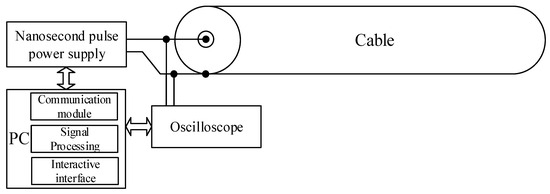
Figure 1.
Cable fault location test platform.
In the test platform (Figure 1), impedance mismatch at the oscilloscope interface can cause secondary signal reflections. These reflections create multiple echoes that distort the waveform and can interfere with the primary reflection from the fault, posing a challenge for accurate peak detection.
The proposed signal processing method inherently mitigates this issue. The local extrema screening strategy prioritizes the two most prominent peaks, which typically correspond to the incident wave and the primary fault reflection, effectively ignoring weaker secondary echoes. Subsequently, the dual-Gaussian model fitting focuses on optimally characterizing these two dominant wave components. Since the secondary reflections are generally lower in amplitude, their influence is minimized during the nonlinear optimization process. Therefore, while perfect impedance matching is desirable, the proposed algorithm provides robustness against the inaccuracies introduced by practical mismatches at the measurement end.
The cable system of rail transit vehicles incorporates various transmission media types, such as coaxial signal lines and wire harnesses, exhibiting significant differences in their wave impedance parameters. Based on electromagnetic wave transmission theory, traveling wave signals encounter impedance discontinuities at cable joints, generating reflected waves with phase inversion. Furthermore, overshoot caused by impedance mismatch between the pulse power supply and the line significantly exacerbates waveform oscillation. The nanosecond-level narrow pulse excitation signal required for short-distance cable fault localization suffers severe attenuation of its high-frequency components during transmission due to the skin effect and dielectric loss. Experimental studies reveal that when the traveling wave transmission distance is excessive, the amplitude of the fault point signal falls below that of the overshoot signal, leading to misjudgment in traditional peak-detection-based localization algorithms. To address this technical bottleneck, this study proposes a signal polarity normalization processing method, applying an absolute value operation to the original voltage signal V(t).
Given that the incident wave and its resultant overshoot signal can only indicate the position of the cable’s incident wave, the overshoot peak should be excluded during peak detection. Furthermore, to denoise the traveling wave measurement signal, this paper employs Gaussian-weighted moving average filtering to smooth Vabs(t) [15].
To accurately identify the peak locations of the incident and reflected waves and overcome the false triggering issue associated with traditional fixed-threshold methods in the presence of overshoot waveforms, this paper proposes a method based on screening local extreme for peak detection, using the following procedure:
Detect differential sign change points: Candidate peak locations are identified at time t + 1 when and . Candidate peaks are then sorted in descending order of amplitude. The first two local maxima are selected, and their time coordinates t1 and t2 are designated as the initial positions of the incident and reflected waves, respectively. This approach prioritizes retaining the incident and reflected waves through extreme sorting, mitigating the risk of missing weak reflected waves caused by signal attenuation.
To address the dispersion effect during traveling wave signal propagation, a double-Gaussian function model is established to characterize the incident and reflected waves:
where A represents the amplitude, denotes the wave peak arrival time, and σ characterizes the Gaussian pulse width; subscripts 1 and 2 correspond to the incident wave and reflected wave, respectively.
To enhance the model’s physical soundness, initial conditions incorporate the peak values and peak times of both waves: the incident wave’s peak position is set to the peak location within the measured signal, while the reflected wave position is assigned to the second highest peak location calculated via Equation (4). Model parameters are solved using a nonlinear least-squares optimization framework, with the objective function defined as minimizing the sum of squared residuals between the observed signal and the model output:
Parameters are iteratively updated via the Levenberg–Marquardt algorithm, dynamically adjusting the damping factor to balance convergence speed and stability. Maximum iterations (1000) and function evaluations (10,000) are capped to ensure global convergence, with termination triggered when the gradient norm threshold falls below 10−6. The optimized parameters and are used to calculate the fault distance:
where v denotes the traveling wave propagation velocity. The accuracy of fault localization is contingent upon the propagation velocity of the electromagnetic wave v, which is related to the per-unit-length inductance L and capacitance C of the cable. In high-frequency applications, v can be considered constant for sufficiently high-frequency components. However, as L and C vary across different cable types, so does the value of v. In this study, for each cable sample, v was determined through a calibration procedure: the time difference Δt between the incident and reflected waves was first measured for a cable with a known fault distance d, and the velocity was then calculated using v = 2 d/Δt. Calibration experiments confirmed that v remained stable for each cable type, with a variation in less than 2%. Consequently, the calibrated v values were employed in the fault distance calculation using Equation (7).
This calibration procedure directly addresses the dependency of the method on the wave velocity, v, which varies with cable type. It provides a practical way for users to accurately determine this critical parameter in advance for any specific cable, irrespective of its length or inherent characteristics (L and C), thereby ensuring localization accuracy in field applications.
The signal processing flow of the proposed method is illustrated in Figure 2. Initially, polarity normalization is applied to the raw voltage signal V(t) via absolute value operation, generating Vabs(t) to eliminate phase inversion interference. Subsequently, Gaussian-weighted moving average filtering smooths and denoises the signal, suppressing waveform distortion induced by high-frequency noise and transmission attenuation. Using the preprocessed signal, candidate peak locations are extracted by detecting differential sign change points. The peak times t1 and t2 for the incident and reflected waves are prioritized through local extremum sorting. Building upon this, a double-Gaussian function model is established. Its peak parameters (A1, μ1, σ1, A2, μ2, σ2) are optimized using the Levenberg–Marquardt algorithm within a nonlinear least-squares framework. Finally, precise fault distance localization is achieved via time-delay calculation based on the optimized peak arrival time difference Δμ = μ2 − μ1 and the traveling wave propagation velocity v. This cascaded workflow—integrating signal preprocessing, feature extraction, and model optimization—effectively overcomes the limitations of conventional methods in scenarios involving overshoot interference and weak reflected waves.
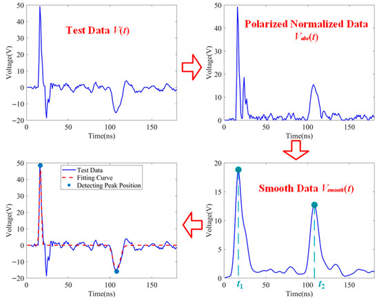
Figure 2.
Cable fault location signal processing flowchart.
3. Experiment
3.1. Fault Experiment on 1 × 1.0 mm2 Single-Core Coaxial Cables
For the 1 × 1.0 mm2 single-core coaxial cable, the wave velocity was determined via calibration as . Traveling wave measurements from 1 × 1.0 mm2 single-core coaxial cable with various open-circuit (Figure 3) and short-circuit (Figure 4) faults at positions (5 m, 10 m, 15 m, 20 m) demonstrate a linear increase in the peak separation between incident and reflected waves with fault distance, validating the proportional relationship between wave time delay and distance. At the 20 m fault distance, the reflected wave amplitude exhibits significant attenuation (~45% reduction compared to the 5 m case) due to skin effect and cable parasitic inductance, causing its peak amplitude to approach that of the overshoot oscillation induced by impedance mismatch in the raw signal. Applying the proposed method—sequential polarity normalization (eliminating phase inversion interference), Gaussian filtering (suppressing high-frequency noise and waveform distortion), and local extrema screening—successfully extracted the dominant peak locations of both waves across all cases. Although the sampling frequency of the experiment is 1 GHz, the non-linear fitting optimization of the double Gaussian model can achieve sub nanosecond estimation of time difference (such as 0.01 ns) based on interpolation, thereby ensuring the improvement of fault localization accuracy. Subsequent nonlinear optimization using the double-Gaussian model quantified the peak arrival time differences for open-circuit faults as 33.51 ns, 62.61 ns, 91.25 ns, and 120.42 ns at 5 m, 10 m, 15 m, and 20 m, respectively. Corresponding differences for short-circuit faults were 33.31 ns, 63.16 ns, 91.45 ns, and 121.78 ns. This approach effectively identified the peak time differences for both fault types.
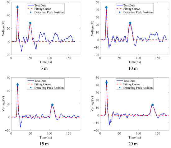
Figure 3.
Traveling wave measurement data and fitting data of cable open circuit fault.
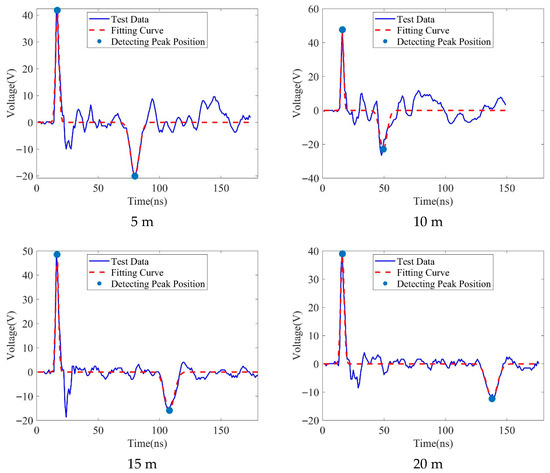
Figure 4.
Traveling wave measurement data and fitting data of cable short circuit fault.
3.2. Fault Experiments on 2 × 0.75 mm2 Dual-Core Coaxial Cables
For the 2 × 0.75 mm2 dual-core coaxial cable, the calibrated wave velocity was . Fault experiments on 2 × 0.75 mm2 dual-core coaxial cable (open-circuit faults: Figure 5; short-circuit faults: Figure 6) revealed more complex traveling wave characteristics, particularly at short fault distance. Strong near-end electromagnetic coupling between the dual cores introduced not only impedance-mismatch-induced overshoot but also superimposed dense crosstalk spikes and high-frequency parasitic oscillations in the raw signal, creating a complex multi-peak background. This coupling effect was especially pronounced at short distances where signal attenuation was insufficient, causing the primary reflected wave peak to be frequently surrounded by dense secondary oscillation, significantly complicating peak identification. Even at longer distances, the attenuated reflected wave’s low-SNR main peak required extraction amidst persistent coupled noise. The proposed method effectively unified the reflection polarity across cores via polarity normalization, while Gaussian filtering preferentially suppressed high-frequency crosstalk spikes. Crucially, the local extrema screening strategy successfully penetrated the complex short-distance multi-peak background and long-distance low-SNR interference, consistently locking onto the primary incident and reflected wave peak locations. Optimization with the double-Gaussian model precisely measured peak arrival time differences for open-circuit faults as 35.63 ns, 63.92 ns, 97.48 ns, and 123.94 ns at 5 m, 10 m, 15 m, and 20 m, respectively. Corresponding differences for short-circuit faults were 36.56 ns, 66.98 ns, 97.31 ns, and 127.69 ns. These results robustly validate the method’s peak recognition capability under strong dual-core coupling interference, effectively handling both short-distance dense oscillations and long-distance weak signals.
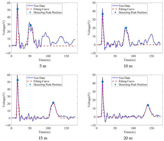
Figure 5.
Traveling wave measurement data and fitting data of cable open circuit fault.
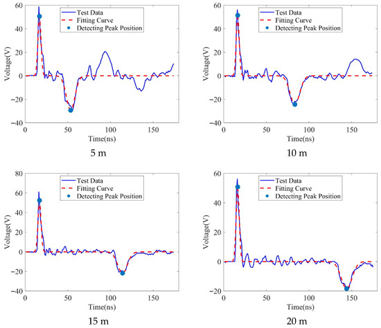
Figure 6.
Traveling wave measurement data and fitting data of cable short circuit fault.
3.3. Fault Experiments on 1 × 1.5 mm2 Wire Harness Cables
For the 1 × 1.5 mm2 wire harness cable, the calibrated wave velocity was . Fault experiments on 1 × 1.5 mm2 wire harness cables (Figure 7) exhibited signal characteristics distinct from coaxial cables. Benefiting from the increased conductor cross-sectional area and the distributed parameter nature of the harness structure, high-frequency crosstalk spikes were significantly reduced compared to dual-core coaxial cables, with background noise manifesting as broad oscillations rather than dense spikes. At the 10 m fault distance, the reflected wave main peak exhibited higher amplitude and relatively clear contour yet was superimposed with significant low-to-medium frequency background oscillations due to harness non-uniformity. At 20 m, reflected wave energy decayed more gradually due to reduced conductor resistance attenuation, though the main peak remained submerged within persistent broad oscillation background. The proposed method eliminated joint phase jumps via polarity normalization, while Gaussian filtering specifically suppressed residual medium-frequency interference. The local extrema screening strategy efficiently locked onto the primary incident and reflected wave peaks amidst the sparsely interfered harness signal. Double-Gaussian model optimization precisely measured peak arrival time differences for open-circuit faults as 63.19 ns and 116.33 ns at 10 m and 20 m, respectively. Corresponding differences for short-circuit faults were 65.29 ns and 120.63 ns.
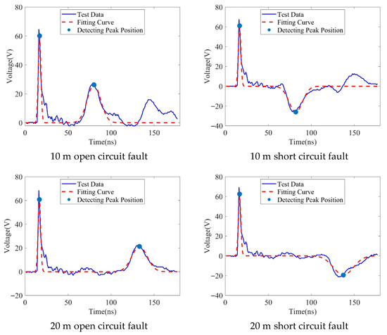
Figure 7.
Traveling wave measurement data and fitting data.
4. Discussion
The theoretical prediction for the time difference between the incident and reflected pulses is given by the fundamental wave propagation equation Δτ = 2d/v, where d is the fault distance and v is the wave velocity. This establishes a strict linear relationship between d and Δτ. For each cable type, the theoretical time differences for the tested fault distances (5 m, 10 m, 15 m, 20 m) were calculated using the respective calibrated wave velocity.
Experimental data from three cable types in Figure 8 demonstrate the core relationship between fault distance and time delay: despite minor deviations between open- and short-circuit measurements (e.g., 63.92 ns for open vs. 66.98 ns for short at 10 m in dual-core coaxial cable, a discrepancy of 3.06 ns), the values strictly adhere to a linear growth trend. This relationship remains robust across cable types and fault scenarios—when fault distance increases from 10 m to 20 m, the time difference rises from 62.61 ns to 120.42 ns (92.3% increase) for single-core coaxial open-circuit faults, and from 65.29 ns to 120.63 ns (84.8% increase) for wire harness short-circuit faults. The slopes of the observed linear relationships closely match the theoretical slope of 2/v for each cable type, as quantified by the low deviations reported above.
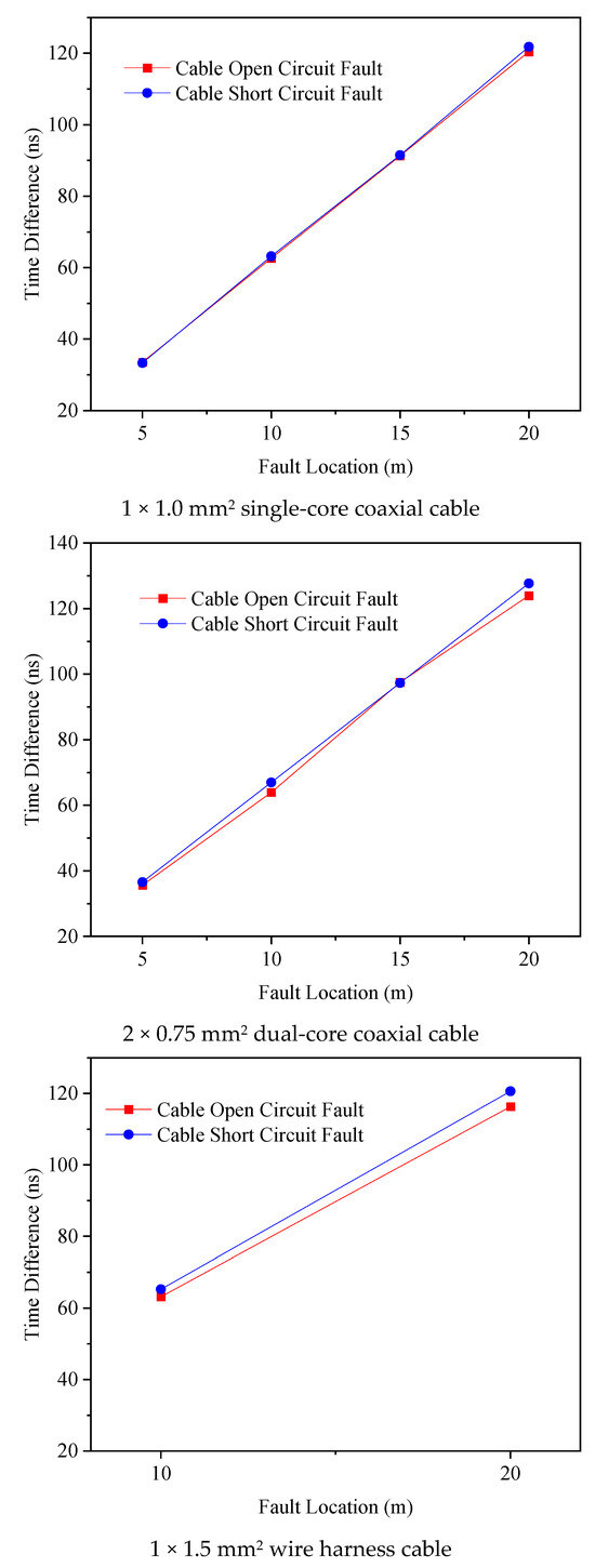
Figure 8.
The echo times of faults in different types of cables.
An observable trend in Figure 8 is that the measured time differences for short-circuit faults are consistently slightly higher than those for open-circuit faults at the same distance across all cable types. This systematic deviation is not a coincidence but can be attributed to the physical differences in the fault point impedance. An ideal short circuit presents a lower impedance discontinuity compared to an ideal open circuit. In practice, a short-circuit fault, especially in complex cable structures, may involve a finite contact resistance and inductance at the fault point. This non-ideal termination causes a more complex interaction with the high-frequency components of the nanosecond pulse, potentially leading to a slight dispersion or a very small additional group delay at the point of reflection. Furthermore, the electromagnetic field distribution around a short-circuit fault differs from that of an open circuit, which can minutely affect the effective propagation velocity of the wave very close to the discontinuity. Although the calibrated wave velocity v accounts for the bulk propagation in the cable, these localized effects at the fault point itself could result in a consistently longer measured round-trip time for short-circuit conditions. The magnitude of this delay difference is small and systematic, which further supports its origin in the fundamental physics of the reflection process rather than being random measurement noise.
The observed data fluctuations precisely highlight the method’s anti-interference strength: despite strong crosstalk in the 10 m short-circuit fault of the dual-core coaxial cable, a reasonable value of 66.98 ns was measured, forming a coherent linear relationship with the 127.69 ns result at 20 m. Although the 20 m open-circuit fault data point (116.33 ns) for the wire harness cable exhibits vertical deviation due to background oscillation, it remains within the overall trend band. A quantitative comparison with theoretical predictions further confirms the method’s accuracy. For the single-core coaxial cable, the measured time differences across all fault distances deviated from the theoretical values by an average of 1.2% and a maximum of 2.5%. Similarly, for the dual-core coaxial cable, the average and maximum deviations were 1.8% and 3.5%, respectively. The wire harness cable exhibited deviations of 2.1% on average and 3.8% at maximum. These consistently low error margins, all below 4%, validate the strong agreement between the experimental results and the theoretical model, as visually evidenced by the linear trends in Figure 8. This demonstrates that the double-Gaussian model optimization effectively filters transient noise while preserving the linear core amidst fluctuations. The minor variations in the figure reflect not methodological shortcomings but authentic responses of the complex cable system—inherent disturbances like joint impedance jumps and electromagnetic coupling are accommodated within the error band by the dual-peak identification process. This capacity to fit imperfect data constitutes the method’s core advantage over traditional peak detection: it prioritizes trend consistency over absolute single-point accuracy, thereby ensuring localization reliability.
The consistent linear relationship observed across all cable types and fault distances, as depicted in Figure 8, further validates the robustness of the proposed method. It demonstrates effective peak identification not only under signal attenuation and overshoot interference but also in the presence of complex waveform distortions, including those potentially arising from practical impedance mismatches in the measurement system.
Regarding the applicability to longer cables, the proposed method possesses inherent robustness against signal attenuation, which is a primary challenge in long-distance fault location. The local extrema screening strategy is designed to prioritize the two most significant peaks, which enables it to capture the incident wave and the dominant reflection even when the latter is substantially attenuated and submerged in noise. This capability is evidenced in our experiments at 20 m, where the reflected wave amplitude was attenuated by approximately 45% compared to the 5-m case, yet the method successfully identified the peaks. The core principle of fault localization via time-difference measurement remains valid regardless of cable length, as long as the reflected wave peak remains identifiable above the noise floor. The observed linearity between time difference and distance (Figure 8) confirms that the wave velocity remains stable, which is a critical precondition for extending the method to longer distances. While the experimental validation in this study focused on the typical cable lengths found within rail transit vehicles, the signal processing methodology itself does not impose a fundamental distance limitation. Future work will involve validating the method on longer cables to explicitly define its operational range and limitations under extreme attenuation scenarios.
To convert the identified bimodal time difference into accurate fault distance, this study follows the following steps for positioning calculation: firstly, the propagation speed v of traveling waves in various cables is obtained through experimental calibration. Then, the proposed traveling wave bimodal recognition method is applied to accurately extract the time difference Δt between the peaks of the incident wave and the reflected wave from the fault signal containing interference. Finally, based on the principle of traveling wave distance measurement, the precise distance L between the fault point and the measuring end is calculated using the formula L = v·Δt/2.
5. Conclusions
This study addresses the critical challenge of accurately locating faults in rail transit train cables under impedance mismatch conditions, which leads to overshoot interference and weak reflected signals. A novel traveling wave dual-peak identification method is proposed and validated. The key conclusions are as follows:
- The proposed method, combining polarity normalization, Gaussian-weighted filtering, local extrema screening, and dual-Gaussian model optimization, effectively overcomes the limitations of traditional peak detection. It successfully isolates the incident and reflected wave peaks even in the presence of significant overshoot, complex crosstalk, and low signal-to-noise ratio.
- Experimental results on single-core coaxial, twin-core coaxial, and harness cables with both open and short circuit faults at various distances demonstrate the method’s effectiveness and robustness. The measured time differences between incident and reflected peaks consistently exhibited a strong linear relationship with the actual fault distance across all cable types and fault scenarios, affirming the fundamental soundness of the approach.
- By precisely quantifying the time difference between the optimized incident and reflected wave peaks and utilizing the known wave velocity, the method significantly improves the accuracy and reliability of fault distance calculation under challenging impedance mismatch conditions that are prevalent in complex rail transit cable systems, irrespective of the specific cable length within the vehicle.
Author Contributions
Conceptualization, C.W. and J.C.; methodology, C.W.; software, J.C.; validation, Y.X., S.Z. and J.L.; formal analysis, Y.X.; investigation, J.H.; resources, J.L.; data curation, C.W.; writing—original draft preparation, J.C.; writing—review and editing, S.Z.; visualization, J.H.; supervision, J.H.; project administration, J.C.; funding acquisition, J.H. All authors have read and agreed to the published version of the manuscript.
Funding
This research was funded by CRRC Technology Project: Development of Rapid Location Device for Rail Transit Cable Fault Points under PMADP.
Data Availability Statement
The original contributions presented in the study are included in the article; further inquiries can be directed to the corresponding author.
Conflicts of Interest
Authors Chongming Wang, Jianhai Chen, Yinqiang Xiang, Shun Zhang and Jinguo Lu were employed by the CRRC Nanjing Puzhen Co., Ltd. The remaining author declares that the research was conducted in the absence of any commercial or financial relationships that could be construed as a potential conflict of interest.
References
- Canudo, J.; Sevillano, P.; Iranzo, A.; Kwik, S.; Preciado-Garbayo, J.; Subías, J. Simultaneous Structural Monitoring over Optical Ground Wire and Optical Phase Conductor via Chirped-Pulse Phase-Sensitive Optical Time-Domain Reflectometry. Sensors 2024, 24, 7388. [Google Scholar] [CrossRef] [PubMed]
- Dong, S.; Yu, F.; Wang, K. Safety evaluation of rail transit vehicle system based on improved AHP-GA. PLoS ONE 2022, 17, e0273418. [Google Scholar] [CrossRef] [PubMed]
- Frosini, P.; Gridelli, I.; Pascucci, A. A Probabilistic Result on Impulsive Noise Reduction in Topological Data Analysis through Group Equivariant Non-Expansive Operators. Entropy 2023, 25, 1150. [Google Scholar] [CrossRef] [PubMed]
- Gültekin, Ö.; Cinar, E.; Özkan, K.; Yazıcı, A. Real-Time Fault Detection and Condition Monitoring for Industrial Autonomous Transfer Vehicles Utilizing Edge Artificial Intelligence. Sensors 2022, 22, 3208. [Google Scholar] [CrossRef] [PubMed]
- Haohao, C.; Jing, L.; Ping, C. Design of fault location algorithm based on online distributed travelling wave for HV power cable. PLoS ONE 2024, 19, e0296513. [Google Scholar] [CrossRef] [PubMed]
- Huo, W.; Qu, Z.; Ao, Z.; Zhang, Y.; Zhao, E.; Zhang, C.; Jiang, H. Fault location of cable hybrid transmission lines based on energy attenuation characteristics of traveling waves. Sci. Rep. 2022, 12, 22448. [Google Scholar] [CrossRef] [PubMed]
- Li, J.; Wang, C.; Zhao, Y. A Long-Term Monitoring Method of Corrosion Damage of Prestressed Anchor Cable. Micromachines 2023, 14, 799. [Google Scholar] [CrossRef] [PubMed]
- Li, J.; Zhao, Z.; Li, L.; He, J.; Li, C.; Wang, Y.; Su, C. A distributed parameter model of transmission line transformer for high voltage nanosecond pulse generation. Rev. Sci. Instrum. 2017, 88, 093514. [Google Scholar] [CrossRef] [PubMed]
- Li, M.; Liu, J.; Zhu, T.; Zhou, W.; Zhou, C. A Novel Traveling-Wave-Based Method Improved by Unsupervised Learning for Fault Location of Power Cables via Sheath Current Monitoring. Sensors 2019, 19, 2083. [Google Scholar] [CrossRef] [PubMed]
- Neumann, T.; Ludwig, J.; Kerkering, K.M.; Speier, P.; Seifert, F.; Schaeffter, T.; Kolbitsch, C. Ultra-wide band radar for prospective respiratory motion correction in the liver. Phys. Med. Biol. 2023, 68, 055021. [Google Scholar] [CrossRef] [PubMed]
- Pal, H.S.; Kumar, A.; Vishwakarma, A.; Lee, H.-N. Electrocardiogram signal compression using adaptive tunable-Q wavelet transform and modified dead-zone quantizer. ISA Trans. 2023, 142, 335–346. [Google Scholar] [CrossRef] [PubMed]
- Xie, W.; Feng, T.; Zhang, M.; Li, J.; Ta, D.; Cheng, L.; Cheng, Q. Wavelet transform-based photoacoustic time-frequency spectral analysis for bone assessment. Photoacoustics 2021, 22, 100259. [Google Scholar] [CrossRef] [PubMed]
- Youn, J.H.; Song, K.Y.; Martin-Lopez, S.; Gonzalez-Herraez, M.; Fernández-Ruiz, M.R. Brillouin expanded time-domain analysis based on dual optical frequency combs. Light. Sci. Appl. 2024, 13, 149. [Google Scholar] [CrossRef] [PubMed]
- Zeng, Z.; Jiang, C.; Zhou, Y.; Zhou, T. A Time–Frequency Domain Analysis Method for Variable Frequency Hopping Signal. Sensors 2024, 24, 6449. [Google Scholar] [CrossRef] [PubMed]
- Houshmand, N.; Esmaeili, K.; Goodfellow, S.; Juan, C. Predicting rock hardness using Gaussian weighted moving average filter on borehole data and machine learning. Miner. Eng. 2023, 204, 17. [Google Scholar] [CrossRef]


Disclaimer/Publisher’s Note: The statements, opinions and data contained in all publications are solely those of the individual author(s) and contributor(s) and not of MDPI and/or the editor(s). MDPI and/or the editor(s) disclaim responsibility for any injury to people or property resulting from any ideas, methods, instructions or products referred to in the content. |
© 2025 by the authors. Licensee MDPI, Basel, Switzerland. This article is an open access article distributed under the terms and conditions of the Creative Commons Attribution (CC BY) license (https://creativecommons.org/licenses/by/4.0/).