Abstract
Single-phase ground faults (SPGFs) in isolated neutral medium-voltage networks are difficult to detect, especially under high transient resistance. This paper proposes a centralized ground fault protection unit (CGFPU) that combines zero-sequence current (ZSC) magnitude and phase-angle analysis to enhance selectivity. Simulation results show that as transient resistance increases from 1 Ohm to 10 kOhm, fault currents decrease significantly, yet the CGFPU reliably identifies the faulty feeder by exploiting the characteristic 180° phase shift of ZSC phasors. The method remains selective with angular deviations up to ±20° and distinguishes between feeder and busbar faults. Compared with conventional amplitude- or model-based techniques, the proposed approach achieves faster detection, lower computational complexity, and robustness against unbalanced and charging currents. Furthermore, the CGFPU operates adaptively in alarm or trip mode depending on fault severity, thus preserving continuity for high-resistance faults and ensuring rapid isolation of bolted faults. These contributions establish a practical, scalable, and future-ready solution for SPGF protection in medium-voltage isolated neutral networks.
1. Introduction
The problem of SPGFs in the MV distribution networks with isolated neutral has been studied extensively, yet it remains one of the most challenging issues in modern power engineering. SPGFs account for the majority of insulation breakdowns in 6–35 kV cable and overhead networks, leading to overvoltages, equipment failures, and difficulties in relay protection operation. Despite decades of research, the accurate detection, localization, and mitigation of SPGFs—particularly under conditions of transient resistance—continue to require further improvement. Zhang et al. [1] investigated faulty feeder selection methods in non-solidly grounded systems and emphasized the practical challenges of discriminating between feeders in distribution networks where capacitive currents dominate fault conditions. In contrast, Ma et al. [2] proposed a voltage phase comparison technique for line protection against SPGFs, demonstrating that phasor-based algorithms significantly improve the speed and sensitivity of fault detection compared to traditional amplitude-based approaches. With the growing use of artificial intelligence, Abbas et al. [3] introduced a neural network-based scheme for SPGF detection and location in the MV networks. Their results showed promising accuracy, but implementation complexity and training data requirements limited industrial application. Building upon this, Mukherjee et al. [4] applied supervised principal component analysis for SPGF localization in transmission systems, thus highlighting the role of advanced data-driven methods for fault identification. Alongside these algorithmic developments, Mardegan and Rifaat [5] discussed the application of IEEE standards for ground-fault protection in industrial and commercial systems. Their work underscored the importance of standardized guidelines but also identified gaps in adapting such recommendations to networks with isolated or compensated neutrals. Complementary to this, Gazprom’s industrial standard [6] provided detailed guidelines on selecting grounding modes for 6–10 kV systems, widely used in Russia and CIS countries, although its recommendations are not always transferable to other operating environments. The influence of transient resistance on SPGF dynamics was analyzed by Ustinov et al. [7], who showed that conventional protections in mining power networks may fail under resistive faults, calling for adaptive methods. Similarly, Kraszewski et al. [8] examined ferroresonance phenomena in voltage transformers, proposing mitigation strategies that are particularly relevant for isolated neutral networks where ferroresonance can exacerbate fault conditions. Overvoltages during SPGFs were the focus of Rzayeva et al. [9], who demonstrated that isolated neutral configurations in 10–35 kV networks experience severe voltage imbalances during SPGFs. Earlier, Shuin [10] investigated the discharge of faulty phase capacitance in 3–10 kV cable systems, forming the theoretical basis for subsequent protection techniques, while Shuin and Gusenkov [11] consolidated these insights in a practical handbook on ground-fault protection. Lin et al. [12] developed selective SPGF protection for ineffectively grounded systems, employing current-voltage correlation principles to increase reliability. Henriksen [13] proposed a charge-voltage method for feeder identification in high-impedance grounded networks, addressing the challenge of low-fault current magnitudes. In parallel, Huang and Wan [14] suggested computational methods to enhance ground-fault analysis accuracy, further enriching theoretical frameworks. Hybrid approaches also emerged, as Lin and Ou [15] proposed fault analysis techniques for unbalanced distribution systems using compensation models, while Ou [16] expanded this to microgrids, demonstrating that unsymmetrical fault analysis is vital for distributed generation contexts. Andreev [17] systematically analyzed existing SPGF protection types, identifying operational boundaries and gaps in applicability. Similarly, Shabad [18,19] produced tutorial and lecture-based materials that provided practical grounding and protection guidelines, still relevant for engineers today. On the broader system level, Andreev [20] and Fedoseyev [21] presented comprehensive treatments of relay protection and automation, framing SPGF issues within the overall protection strategy. At the experimental and applied level, Vinokurova et al. [22] studied operating frequency ranges for SPGF protection in cable networks, showing that transient process analysis allows the refinement of relay settings. Hänninen [23] contributed a fundamental study on SPGFs in high-impedance networks, covering their characteristics, indication, and localization, widely referenced in Nordic countries. Earlier works by Gelfand [24] and Evdokunin et al. [25] explored neutral grounding choices, with practical implications for fault current limitation. The selection of grounding modes has remained a critical theme. Titenkov and Pugachev [26] discussed neutral grounding schemes in 6–35 kV systems, while Weinstein et al. [27] offered a tutorial on neutral modes with pedagogical clarity. Yemelyanov and Shirkovets [28] focused on resistive and combined grounding, identifying current issues in Russian practice. Khalilova and Boynazarov [29] analyzed arc-suppressing reactors for capacitive fault current compensation, showing their effectiveness but also design limitations. More recently, Shirkovets et al. [30] evaluated resistive grounding applications in XLPE cable networks, highlighting compatibility concerns, and Ilyinykh et al. [31] proposed compensated and combined grounding methods, underlining their benefits for reducing fault current magnitudes while preserving reliability. In summary, the literature reveals substantial progress in understanding SPGF mechanisms, protection methods, and grounding strategies. However, several limitations persist: (i) many techniques lose sensitivity in the presence of high transient resistance; (ii) most models neglect non-linear interactions between capacitive and resistive fault components; and (iii) standardization remains fragmented across regions. These gaps justify the present study, which analyzes SPGF behavior in 10 kV networks with isolated neutral, focusing on the impact of transient resistance on ground-fault currents, zero-sequence voltages, and feeder responses.
Lu et al. [32] developed the non-crossing sparse-group Lasso-quantile regression deep neural network (SGLQRDNN) for probabilistic load forecasting, enforcing non-crossing quantile constraints and applying sparse-group regularization to stabilize feature selection, thereby delivering consistent quantile trajectories and improved robustness for renewable-dominated grids. Lu et al. [33] then proposed a class-imbalance privacy-preserving federated learning (CI-PPFL) framework for decentralized fault diagnosis, combining differential-privacy noise injection with adaptive class-imbalance reweighting and biometric authentication to enable secure, cross-site model training without sharing raw data. Complementing these advances, subsequent work of Zhang et al. [34] extended non-crossing quantile regression into deep architectures, further reducing quantile crossings and tightening predictive intervals under non-stationary load profiles. Wang et al. [35] applied federated learning to electricity-theft detection across heterogeneous clients, demonstrating privacy-preserving inference that remains resilient to distribution shifts among utilities. For operational control, recent studies [36] employed deep reinforcement learning to co-optimize microgrid dispatch, reserves, and demand response under renewable uncertainty, improving multi-objective performance relative to rule-based baselines. Finally, comprehensive surveys [37] synthesize these threads—architectural patterns, optimization strategies, and AI-driven control—while identifying outstanding challenges in scalability, interoperability, data governance, and cyber-security for next-generation smart grids.
2. Materials and Methods
To achieve the objectives of this study, the following research tasks were undertaken:
- Analyze the influence of transient resistances during SPGFs on the performance of protection systems.
- Assess the operation of protection systems under various transient resistance conditions to determine sensitivity, selectivity, and reliability.
- Develop a selective protection scheme and algorithm capable of reliably detecting and protecting the MV networks against SPGFs under different neutral grounding modes.
2.1. Research Framework
The research methodology is based on a comprehensive analysis of 6–35 kV distribution networks, considering both the statistical occurrence and physical nature of SPGF events. The study integrates simulation modeling, fault event analysis, and comparative evaluation of several relay protection techniques.
Disturbance records obtained from actual fault events in 6–10 kV substations were analyzed to validate the model and ensure representativeness of transient processes. A detailed review of existing protection principles—including harmonic-based, directional overcurrent, and transient-based methods—was conducted to identify their strengths, limitations, and areas requiring improvement.
2.2. Simulation Model
A 10 kV network model with two substations and six outgoing feeders was developed using MATLAB Simulink R2024b (The MathWorks Inc., Natick, MA, USA).
SPGFs were applied sequentially at different locations (bus and feeders) with transient resistance varying from 1 Ohm to 10 kOhm, allowing analysis of protection response under resistive and capacitive fault conditions.
2.3. Implementation of the CGFPU
The CGFPU uses a centralized measurement of ZSC from each feeder and identifies an SPGF at the feeder or on the bus based on the angle and magnitude comparison. To enhance reliability:
- Thresholds and trip settings were aligned with the Rules for Electrical Installations of the Republic of Kazakhstan (PUE RK) No.230 and IEC 60255 standards [38].
- Only current signals were required, minimizing communication and instrumentation costs.
3. Comparative Analysis of the Existing Protection Methods
Relay protection in the MV networks generally relies on one or more of the following criteria:
- -
- Harmonic-based protection uses the characteristic of the third and fifth harmonics of the residual current/voltage which are excited by intermittent arcs restrikes or ASR detuning.
- -
- Directional overcurrent protection uses directional element zero sequence current and voltage or negative-sequence with an overcurrent pickup; classic feeder-local protection.
- -
- Transient based protections extract high-frequency or first-cycle features (dU0/dt, dI0/dt, wavelets) at the fault inception or re-ignition.
- -
- Proposed CGFPU uses a centralized method of zero-sequence current angle and magnitude comparison across feeders.
Table 1 shows the comparative analysis of the existing protection methods and the proposed CGFPU.

Table 1.
Protection scheme comparison.
Table 2 shows the protection criteria which set the requirements such as sensitivity speed, selectivity, robustness, noise, and communications need.
Table 2.
Protection criteria.
Table 3 shows the complexity and lifecycle cost.
Table 3.
Complexity and lifecycle cost.
Results summary
General disadvantages of modern protection methods:
- -
- Non-selective operation in the event of SPGF under different stability conditions.
- -
- Probability of failure to operate in case of SPGFs with high transient resistances, decreased sensitivity.
- -
- High cost, complexity of design and operation.
- -
- Auxiliary signals such as zero sequence voltage, higher harmonics, etc., are required for the protection functioning.
The proposed CGFPU is the most effective because it is selective, performs both angle and magnitude comparisons, is sensitive to various transient resistances, and operates quickly (within 20–40 ms). It is robust and reliable under different transient processes and noise conditions, and cost-effective since it uses only the zero-sequence current. No additional polarization or auxiliary signals or equipment are required. Moreover, it is universal, as the proposed protection can be used in three modes: isolated, compensated, and high-resistance grounded neutral configurations.
4. Impact of the Transient Resistance on the SPGF Fault Levels
The presence of transient resistance during an SPGF leads to a reduction in protection sensitivity, thereby undermining the reliability and efficiency of MV networks configured with isolated neutrals. In practice, incomplete ground faults are frequently accompanied by transient resistance, which can range from a few Ohms to several kilo-Ohms [7,18]. These resistance values are random and depend on various factors, such as the presence of moisture, icing, tree branches, and the soil’s specific properties. During SPGFs with transient resistance, the magnitudes of zero-sequence current and voltage are significantly reduced. Since the settings for ground overcurrent protections are typically calculated assuming bolted faults (i.e., near-zero resistance faults), the failure to account for transient resistance may result in the protection system failing to detect and isolate the fault [10,11,20]. Moreover, transient resistance affects not only traditional ground overcurrent protections but also protections based on detecting higher harmonic components in the steady-state SPGF current. Studies show that transient resistances of just a few Ohms can lead to substantial sensitivity degradation [11,21]. Directional overcurrent protections that determine the direction of zero-sequence current under steady-state fault conditions offer somewhat better performance. Nonetheless, analysis reveals that even these protections exhibit low selectivity for SPGFs when transient resistances reach values between 600 and 700 Ohms, particularly in networks with a maximum distributed capacitance of around 6.5 μF. Figure 1 illustrates the relationship between SPGF conditions and transient resistance values for soils with high specific resistivity [7,29].
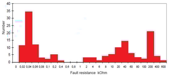
Figure 1.
Distribution of the number of SPGFs versus transient resistance values at the fault location in a 10 kV network [23].
The statistical distribution in Figure 1 illustrates the occurrence of SPGFs with respect to transient resistance at the fault location. The data confirm that most faults fall within the range of 0.02–200 kOhm, though with two distinct clusters.
- A large proportion of faults occur at very low resistance values (<0.1 kOhm), which typically generate sufficiently high fault currents to be detected by conventional protection systems.
- Another significant group of faults is concentrated at higher resistance levels (20–400 kOhm), with a notable peak near 200 kOhm.
- Only a limited number of faults occur in the intermediate resistance range (0.2–10 kOhm).
This uneven distribution highlights the random nature of transient resistance during SPGFs. It also emphasizes the challenge for conventional protection systems: while low-resistance faults are readily detectable, high-resistance faults lead to significant attenuation of zero-sequence currents, reducing the sensitivity and selectivity of existing protections. Therefore, the analysis underscores the necessity of developing advanced algorithms that remain effective across the full spectrum of transient resistance values.
4.1. Defining the Transient Resistance Values at the SPGF Location and Ground Overcurrent Settings
We analyze a single-phase ground fault (SPGF) occurring on phase A through a transient resistance R. The effect of this resistance is introduced via its conductivity in the following:
The nodal equation at the fault point is written in terms of the phase electromotive forces EA, EB, EC, the neutral displacement voltage UN, and admittances of the phases to ground as follows:
where YA, YB, YC—phase admittances,
Gtr—conductivity of the transient resistance,
UN—voltage shift of the neutral point due to the asymmetry.
Rearranging Equation (1) gives the expression for :
where —the phase EMF, —operator of symmetrical components.
If we assume the network is symmetrical, then YA = YB = YC = Yph. Substituting into Equation (2):
Thus, the neutral displacement voltage reduces to
Continuing from the expression for the neutral point voltage displacement, we can reduce Equation (4) to the following form:
where —active phase-to-ground conductance,
—phase-to-ground capacitance.
—transient resistance, Ohm.
ω—angular frequency of the system.
Thus, the neutral shift increases as the transition resistance decreases. As the transient resistance at the fault location decreases, the neutral voltage increases. When , that is, in the case of a solid (metallic) fault, the neutral voltage reaches its maximum value, which equals the phase electromotive force. In this case, the phase-to-ground voltages during a single-phase ground fault can be expressed as follows:
- For the faulty phase A, the voltage becomes
- For the intact phases B and C, it is as follows:
The total ground fault current is obtained as the sum of phase currents as follows:
—Ground fault current, A.
Since , substituting yields
Figure 2 shows the Equivalent zero-sequence diagram for SPGF.
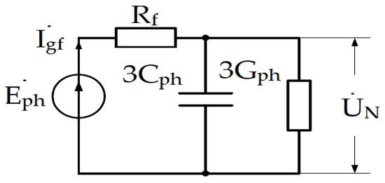
Figure 2.
Equivalent zero-sequence diagram for a single-phase-to-ground fault.
The equivalent zero-sequence circuit of SPGF with the transient resistance Rf is shown in Figure 2. The system consists of the phase electromotive force Eph, fault resistance Rf, phase-to-ground capacitances 3Cph, and leakage conductance 3Gph. The neutral displacement voltage is denoted by UN, and the ground fault current by If. Figure 3 shows dependence of the relative fault current magnitude on the transient resistance value Rf. Here denotes the fault current for Rf = 0.
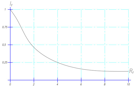
Figure 3.
Graph of the dependence of the ground fault current on the transient resistance.
The ground fault current can be represented as the sum of two components: active component and capacitive component .
Using the previously introduced relative value of the total active conductance of the network phases (d), the absolute value of the fault current for Rf = 0 can be expressed as follows:
The single-phase ground fault current through the transient resistance can also be determined using the capacitive components. During transient processes associated with SPGFs, the ratio between the higher harmonic currents and the fundamental frequency current 50 Hz remains approximately constant [24]. The relationship between zero-sequence voltage and current is expressed as
where I0(t) is zero-sequence current at the SPGF location.
u0(t)—zero-sequence voltage.
C0Σ—the total phase to ground capacitance of the network.
The current I0 through unfaulted lines is determined by their self-capacitance as follows:
where C0s is the self-capacitance of the phase shorted to the ground.
Thus, the total cumulative zero-sequence current during an SPGF can be written as follows:
For the root mean square (RMS) values, integrating over time T, the expressions are
where 3I0(t), 3I0f(t) are the current rms values of zero-sequence currents in the fault mode, —represents the derivative (rate of change) of the zero-sequence voltage.
The steady-state zero-sequence voltage , considering transient resistance , is as follows:
where Uph—the phase-to-ground voltage, V,
U0—the zero sequence voltage, V,
—total phase-to-ground capacitance of the network, F,
—the loop integrity coefficient.
The loop integrity coefficient β is defined as
that is, the ratio of the magnitude of neutral displacement under finite fault resistance Rf to that under a solid fault (Rf = 0). In other words, Loop integrity coefficient β is the value that characterizes how completed a SPGF is, and it quantifies the-so called “completeness” of the fault-current loop formed by the faulted phase and transient resistance.
β ≈ 1: the loop is completely closed (bolted fault), and the neutral voltage is close to the phase voltage.
β < 1: the loop is weakened (higher transient resistance Rf), the neutral displacement decreases, and fault identification becomes more difficult.
β = 0: extremely high transient resistance Rf, the neutral displacement becomes high negligible.
Thus, the zero-sequence fault current becomes
where IC∑ is the total capacitive current of the network in the unfaulted state.
In networks with the isolated neutral configurations, the ground fault current is determined by the difference between total capacitance and the capacitance of the faulted phase. Based on the Equations (15) and (16), the RMS zero-sequence current are
From the derived expressions, the operational current setting for ground fault protection is determined by
where Koff is the offset coefficient accounting for measurement and calculation inaccuracies [11].
As per PUE RK No.230, in our protection setting calculations we consider the sensitivity ration Ks.
The sensitivity ratio of ground fault protection is
where Ks defines the ability of the protection to reliably detect an SPGF even under varying transient resistance conditions.
is the minimum fault current at the end of the protected zone.
The sensitivity ratio, Kₛ is the ratio between the minimum SPGF current at the end of the protected area and the relay’s pickup current. The sensitivity ratio shows how reliably a relay can detect a fault in the most unfavorable conditions, for instance, power system instability, weak power source, fault resistance, etc.
If —the relay may not operate.
If —borderline operation (possible non-operation under variations).
If —reliable and stable operation.
The sensitivity factor Ks and loop integrity coefficient significantly influence protection performance.
The abovementioned equations provide the theoretical framework for determining relay protection settings in MV isolated-neutral networks, ensuring reliable SPGF detection under varying transient resistance conditions.
4.2. Admittance Symmetry Assumption
We will briefly discuss the conditions under which the admittance symmetry assumption occurs, review estimation errors and analysis of the loop integrity ratio, β under different system capacitance, short-circuit capacity, and other conditions.
When the assumption is valid:
- Cable lines for instance three-core cables with symmetric disposition: the phases are located uniformly and the phase-to-ground capacitances are equal.
- Overhead lines with conductor transposition: due to the periodic exchange of conductor positions, the average admittances of the phases are equalized.
- When the assumption cannot be valid:
- Overhead lines without transposition: the phases are positioned asymmetrically on the tower → YA ≠ YB ≠ YC.
- Mixed cable with overhead lines: part of the route is cable, part is overhead.
- Long, untransposed overhead lines in rural networks, where the phase capacitances may be significantly different.
We adopted the symmetry Ya = Yb = Yc as our scheme, which is balanced, with cable lines with almost equal lengths to simplify the calculations.
4.3. Impact of Admittance Imbalance on Neutral Voltage, Transient Resistance, SPGF Errors
Admittances were varied such that YB = Y0(1 + δ), YC = Y0(1 − δ) with δ = 0–15%.
Table 4 shows the results when the system admittance is fully symmetrical (ΔY = 0%). It is used as the baseline case for error comparison. Since the system is balanced, deviations in UN remain negligible across the entire fault resistance range.
Table 4.
Results of the analysis of the neutral displacement voltage, SPGF current errors, transient resistances at the admittance imbalance ΔY = 0%.
Table 5 corresponds to a moderate imbalance scenario (ΔY = 5%). It highlights the first appearance of sensitivity in the neutral displacement voltage. Errors exceed 10% once Rf surpasses ~1 kOhm, illustrating how even small deviations from symmetry can significantly impact protection performance in high-resistance fault cases.
Table 5.
Results of the analysis of the neutral displacement voltage, SPGF current errors, and transient resistances at the admittance imbalance ΔY = 5%.
Table 6 shows the results under a higher imbalance level (ΔY = 10%). The error in neutral displacement voltage increases rapidly, exceeding 25% for Rf ≥ 1 kOhm and approaching 35% at 10 kOhm. Fault current deviation remains negligible (<0.5%).
Table 6.
Results of the analysis of the neutral displacement voltage, SPGF current errors, and transient resistances at the admittance imbalance ΔY = 10%.
Table 7 presents the extreme imbalance case (ΔY = 15%). It demonstrates the largest divergence between the general and symmetric admittance assumptions. Errors in neutral displacement voltage surpass 50% for very high fault resistances (Rf ≥ 9 kOhm). Fault current remains unaffected, confirming that the primary sensitivity lies in UN.
Table 7.
Results of the analysis of the neutral displacement voltage, SPGF current errors, and transient resistances at the admittance imbalance ΔY = 15%.
Figure 4 shows the graph of neutral displacement voltage error (%) against transient fault resistance (Rf) for ΔY = 0%, 5%, 10%, and 15% at 10 kV with the simulation time step of 0.001 s. It clearly illustrates how error grows with both fault resistance and admittance imbalance, with ΔY = 5% already producing >10% error and ΔY = 15% exceeding 50% at high Rf.
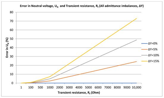
Figure 4.
Error in UN (%) against admittance imbalance and transient resistance at 10 kV with the time step of 0.001 s.
Figure 5 displays the graph of SPGF fault current error (%) for all imbalance cases ΔY = 0%, 5%, 10%, and 15% at 10 kV with the simulation time step of 0.001 s. Across all fault resistances and ΔY values, the error remains very small (<0.5%), confirming that fault current calculation is robust to admittance imbalance.
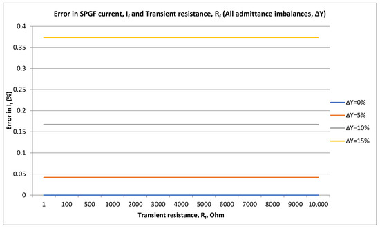
Figure 5.
Error in If (%) against admittance imbalance at 10 kV with the time step of 0.001 s.
4.4. Sensitivity to Network Parameters
- Sensitivity to fault resistance Rf: Loop integrity coefficient β decreases with increasing Rf. For Rf > 5 kOhm the Loop integrity coefficient β drop will increase, explaining the challenge of identifying high-resistance SPGFs.
- Sensitivity to system capacitance C0: the larger capacitance C0 increases the charging current Ic and slows the decay of the loop integrity coefficient β, improving protection detection margins.
- Sensitivity to system voltage Vph: the lesser the system voltage, the lesser charging current and capacitive current accordingly will be during SPGF.
- Sensitivity to short-circuit capacity Ssc: Loop integrity coefficient β shows only weak dependence on Ssc; the angle-based discrimination remains robust from 20 to 80 MVA. As the short circuit capacity has very little effect on the SPGF level, we will consider other aspects.
4.5. Impact of Capacitance and Neutral Voltage on Transient Resistance
The impact of transient resistance on the SPGF behavior is strongly affected by the total network capacitance. At low capacitances, neutral displacement voltage UN remains small, and fault current If quickly decreases as the transient resistance increases, which makes high-resistance faults difficult to detect. In contrast, higher capacitances amplify the effect of transient resistance, producing larger UN values even when the SPGF If is very small. This means that in large-capacitance networks, voltage-based protection elements remain effective for high-resistance faults, while in low-capacitance systems, current-based elements dominate for low-resistance faults but may fail to detect weak ground faults.
Figure 6 shows that for a given Rf, larger Ctot yields higher UN. Physically, a larger network capacitance provides a stronger capacitive coupling of all three phases to ground, which increases neutral shift under asymmetry created by the fault. The analysis was made at 10 kV with the simulation time step of 0.001 s.
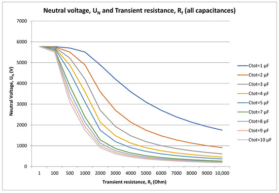
Figure 6.
Dependence of capacitance and neutral voltage from transient resistance at 10 kV with the time step of 0.001 s.
Curves diverge most between about 0.5 and 5 kOhm, where the balance between the fault path and capacitive paths changes rapidly. At very low transient resistance Rf near 1 Ohm, all curves are low and close together; at very high transient resistance Rf ≥ 5–10 kOhm, UN rises significantly.
4.6. Standard Comparison
The CGFPU protection scheme uses fundamental zero-sequence quantities (3I0) with definite-time logic and pickup—this matches the IEC 60255 framework for relay functional behavior.
The CGFPU pickup settings for alarm and trip commands are in accordance with PUE RK No.230, Chapter 2 “Power Supply and Electric Networks,” Section 2 “General Requirements”. Compensation of the capacitive SPGF shall be applied when the value of this current in normal operating conditions is as follows:
- -
- in 3–20 kV networks that have reinforced-concrete and metal supports on overhead lines (OHL), and in all 35 kV networks—more than 10 A;
- -
- in networks that do not have reinforced-concrete and metal supports on OHL: at 3–6 kV—more than 30 A; at 10 kV—more than 20 A; at 15–20 kV—more than 15 A;
- -
- in 6–20 kV generator–transformer block schemes (at generator voltage)—more than 5 A.
In accordance with the above, we shall adopt that for SPGF of 30 A at 6 kV, 20 A at 10 kV, and 10 A at 35 kV, the protection action is alarm; when the above values are exceeded, the protection shall trip.
Basis for delay configuration
Persistence (n-of-m): three to five half-cycles (30–50 ms) on both angle and magnitude to reject restrikes, CT saturation bursts, and cap-bank switching.
Operate times:
- -
- Feeder trip: 80–150 ms definite time after persistence (keeps sub-cycle selectivity, allows security).
- -
- Bus trip (incomer): ~100 ms when all feeders align (bus-fault signature).
- -
- Alarm stage: immediate or 100–150 ms (100 ms for SCADA).
- -
- Angle bands: faulted feeder if |Δφ| ≥ 160° vs. the healthy cluster; bus fault if cluster alignment ≤ 20°.
Table 8 shows the Fault current, If, A and transient resistance, Rf.
Table 8.
Fault current, If, A and transient resistance, Rf.
Figure 7 displays the Fault current, If, A and transient resistance, Rf. The analysis demonstrates a strong inverse relationship between the fault current amplitude and the transient resistance at the point of SPGF. As the transient resistance increases from 1 Ohm to 10 kOhm the magnitude of the fault current decreases sharply. This decline is most pronounced within the range of 1 Ohm to approximately 1000 Ohm, after which the current reduction becomes gradual and eventually stabilizes at low values for all capacitance levels.
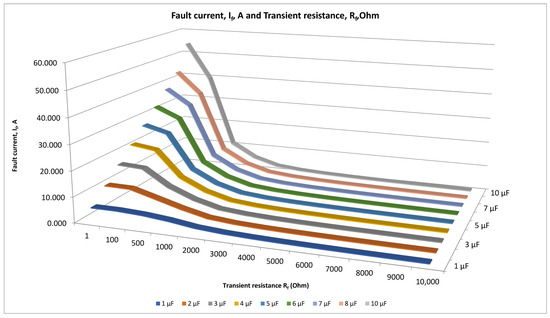
Figure 7.
SPGF current, If, A and transient resistance, Rf at 10 kV with the time step of 0.001 s.
For networks with lower total phase-to-ground capacitance , the fault current remains relatively small across all resistance values, indicating limited energy discharge during ground faults. As the network capacitance increases to 5–10 µF, the initial fault current at low resistances rises significantly-reaching about 50–60 A-before falling rapidly with growing resistance. This trend highlights the combined effect of network capacitive charging and transition resistance on the zero-sequence current magnitude.
At high resistance levels above 5000–6000 Ohm, the differences in fault current between various capacitance values become minimal. This suggests that beyond a certain threshold of transient resistance, the influence of system capacitance on the fault current becomes negligible. Consequently, under such high-resistance fault conditions, traditional current-based protection methods lose sensitivity and may fail to operate reliably.
Table 9 shows the ground overcurrent settings for various transient resistances.
Table 9.
Ground overcurrent settings for various transient resistances.
Figure 8 displays the ground overcurrent settings for various transient resistances at 10 kV with the simulation time step of 0.001 s.
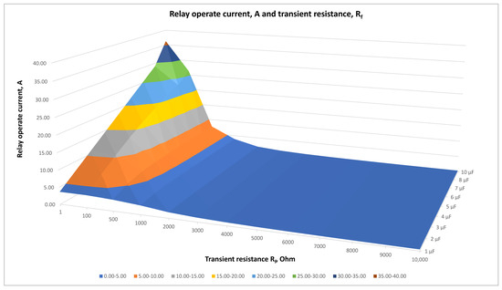
Figure 8.
Ground overcurrent settings for various transient resistances at 10 kV with the time step of 0.001 s.
It illustrates how the pickup current settings of ground overcurrent protection vary depending on the network’s total phase-to-ground capacitance and the transient resistance at the fault point.
The results indicate that the pickup current decreases sharply as the transient resistance increases. For low resistance values (1–500 Ohm), the pickup current is relatively high, reflecting the higher magnitude of zero-sequence currents that appear during strong ground faults. As the transient resistance rises above approximately 1 kOhm, the pickup current values drop rapidly and eventually stabilize at very low levels once exceeds about 4000–5000 Ohm.
At a capacitance of 1 µF, the pickup current remains below 4 A, showing that smaller networks with low capacitive coupling generate weaker zero-sequence components. As the total capacitance increases to 10 µF, the pickup setting required for reliable operation grows significantly-reaching approximately 35–40 A for faults with very low transition resistance. This correlation demonstrates that the protection pickup must be scaled in proportion to the system’s capacitive charging current to maintain sensitivity.
Beyond 5000–6000 Ohm, all pickup current curves converge to nearly identical low values (≈0.4 A), regardless of capacitance. This indicates that under high-resistance SPGF conditions, the influence of network capacitance becomes negligible, and the fault current is dominated by the resistive path through the fault.
Table 10 shows the Loop integrity coefficient, β and transient resistance, Rf.
Table 10.
Loop integrity coefficient, β and transient resistance, Rf.
Figure 9 shows the Loop integrity coefficient, β and transient resistance, Rf. It presents the variation of the loop integrity coefficient, β as a function of transient resistance, Rf for different values of total network phase-to-ground capacitance, . The analysis was made at 10 kV with the simulation time step of 0.001 s.
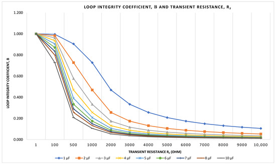
Figure 9.
Loop integrity coefficient, β and transient resistance, Rf at 10 kV with the time step of 0.001 s.
At very low transient resistances 1–100 Ohm, the loop integrity coefficient remains close to unity for all capacitance values, indicating that the network loop is nearly intact and the fault current path is continuous. As the transient resistance increases beyond approximately 500 Ohm, β begins to decline rapidly, reflecting the increasing discontinuity in the fault circuit. This decline is steeper in networks with larger total capacitance, where the capacitive current component decays faster as resistance rises.
For small capacitance values 1–2 µF, the coefficient decreases more gradually, remaining above 0.6 up to around 1000 Ohm. In contrast, networks with higher capacitance 8–10 µF show a much faster deterioration, with β dropping below 0.3 at roughly the same resistance level. Beyond 3000–4000 Ohm, the coefficient values for all capacitances converge toward very low levels, typically below 0.1, indicating that the fault loop is effectively open and the zero-sequence current becomes negligible.
Figure 10 shows the sensitivity factor during SPGF with various transient resistance, Rf at 10 kV with the simulation time step of 0.001 s. It presents the variation of the sensitivity ratio, Ks for different network capacitances and transient resistances. The results demonstrate that the sensitivity ratio remains virtually constant at a value of approximately 1.5 across all examined conditions, regardless of the total network capacitance, or the transient resistance, .
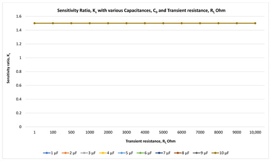
Figure 10.
Sensitivity factor evaluation at 10 kV with the time step of 0.001 s.
This stability indicates that the proposed protection scheme maintains a consistent level of sensitivity under both low- and high-resistance fault conditions. The independence of from confirms that the algorithm’s operating criterion-based on the comparative phase and magnitude of zero-sequence currents is robust and not significantly influenced by variations in the fault impedance or network capacitive current.
Unlike traditional directional or overcurrent protections, which typically show declining sensitivity as the fault resistance increases, the CGFPU maintains a uniform detection threshold, ensuring reliable operation even in the presence of weak fault currents. This behavior verifies that the designed settings and logic conform to the recommended sensitivity range of as defined by the PUE RK, thereby satisfying the requirements for dependable protection performance.
4.7. Similarities with the International Standards
The CGFPU uses power-frequency phasors of zero-sequence quantities and definite-time logic which aligns with IEC, IEEE measuring and timing concepts, provides alarm and trip stages and security measures consistent with standards’ emphasis on security before tripping and also it supports multiple neutral grounding regimes—isolated, compensated, resistive matching the neutral-mode coverage in DL/T practice.
Innovation points
- -
- Centralized selectivity by cross-feeder comparison: the method identifies the faulty feeder by the ~180° opposition of its zero sequence currents to the nearly aligned unfaulted feeders’ capacitive currents and validates with magnitude or when the SPGF is on the bus by 0° alighnment of all unfaulted feeders. This inter-feeder angle clustering is not a requirement in IEC or IEEE and is the core novelty that preserves sensitivity at high transient resistances Rf.
- -
- In copper-wired architecture no time-sync or process-bus is required; the CGFPU receives analog 3I0 from all feeders and decides centrally—simple to retrofit where IEC 61850 is unavailable.
- -
- Adaptive thresholds with persistence: use n-of-m cycle validation to reject switching/noise while keeping pickup at very low zero sequence current magnitudes, and high-resistance faults.
Although the proposed CGFPU method exhibits high accuracy and robustness in simulation studies, several practical aspects should be considered for real-world implementation. One potential challenge is the influence of measurement noise and ZSCT errors, which may distort the zero-sequence current used by the device. To address this, the CGFPU algorithm incorporates digital filtering techniques and to suppress transient noise and offset from the errors while maintaining sensitivity. Another challenge is the parameter variation in distribution networks, such as fluctuating load conditions, network configurations or grounding mode changes, which can affect fault detection reliability. This issue can be mitigated by selecting offset values and predefined settings for various grounding modes within the device parameter settings. Additionally, the integration of CGFPU into existing protection systems requires compatibility with current communication protocols and coordination with traditional ground overcurrent directional relays. Therefore, the CGFPU should be integrated into the communication protocol used and coordinate with the existing relay protection to ensure a smooth transition and enhance system reliability. Overall, these considerations demonstrate that the proposed method is technically feasible and adaptable for field application with appropriate hardware optimization.
Improvement points
High-resistance ground faults: when the transient resistance Rf ≫ 1 kOhm and the ZSC becomes small, conventional feeder-local non-directional, directional elements lose pickup. The cross-feeder angle opposition remains observable and keeps selectivity, so alarms/trips remain dependable at Rf in the 5–10 kOhm range across C0Σ = 1–10 µF.
Bus-fault recognition: the method naturally classifies bus faults when all feeder 3I0 phasors align (no 180° split), enabling fast incomer action without extra logic.
Application in existing protection configurations
Per-feeder zero sequence currents from ZSCT, secondary wiring with not less than 2.5 mm2 for ZCTSs as per PUE RK, Order No.230 and control cables 2.5 mm2 for the direct transfer trip, microprocessor based CGFPU. No new primary equipment required.
Feasibility
The CGFPU works with conventional ZSCTs and wiring; no station time-sync is required; compute burden is modest, persistence logic.
The selectivity is strong for SPGF anywhere on the bus/feeder, including hightransient resistance Rf cases.
Limitations
Large substations with many feeders increase wiring complexity and input-channel count. It willl be required to consider sectionalizing or a networked IEC 61850—GOOSE [39] variant if growth is expected.
4.8. Applicability of the CGFPU in Various Neural Grounding Modes
The CGFPU has a universal application and can operate in various grounding modes with various transient resistances, Rf and various capacitances, C0. Table 11 shows the parameters for analyzing the CGFPU operation in various neural grounding modes.
Table 11.
Parameters.
Table 12 shows the SPGF current, If, A, and transient resistance, Rf for isolated neutral.
Table 12.
SPGF current, If, A, and transient resistance, Rf for isolated neutral.
Figure 11 displays the SPGF current for the isolated neutral network. The ZS current is highest at very low resistance and falls steadily as resistance rises. The biggest drop is from a few hundred Ohms to a few kOhms; by 5–10 kOhms the current is small and changes slowly.
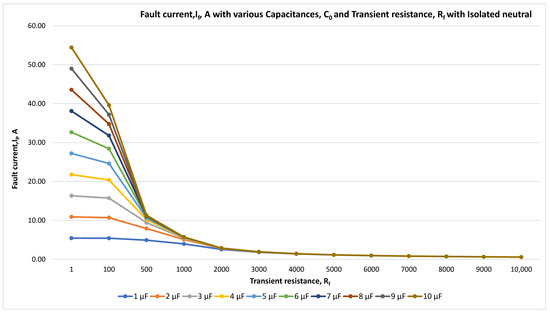
Figure 11.
Fault current, If, A, and transient resistance, Rf for isolated neutral at 10 kV with the time step of 0.001 s.
Table 13 shows the SPGF current, If, A, and transient resistance, Rf for the compensated neutral system with the ASR set undercompensated.
Table 13.
SPGF current, If, A, and transient resistance, Rf for compensated neutral, 0.9 ASR under compensation tuning.
Figure 12 shows SPGF for the compensated neutral system with the ASR set undercompensated. The analysis was made at 10 kV with the simulation time step of 0.001 s. It displays the ZS current drops steadily as the resistance increases; the biggest fall is from a few Ohms to a few kOhm, then it flattens. Compared with the isolated neutral, the ASR greatly reduces current at the low–mid resistances; at the high resistances both modes converge to the same small current.
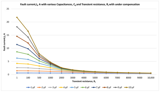
Figure 12.
Fault current, If, A, and transient resistance, Rf for compensated neutral with under compensation at 10 kV with the time step of 0.001 s.
Table 14 shows the SPGF current, If, A, and transient resistance, Rf for compensated neutral with under compensation.
Table 14.
SPGF current, If, A, and transient resistance, Rf for compensated neutral, 1.0 ASR tuning.
Figure 13 displays SPGF for the compensated neutral system with the ASR set compensated. The analysis was made at 10 kV with the simulation time step of 0.001 s. The ZS current drops steadily as the resistance increases, the biggest fall from a few Ohms to ~2–3 kOhms, then it flattens at small values. At low resistance the ZS current rises with capacitance; as resistance moves into the hundreds of Ohms and a few kOhms, that dependence weakens; at high resistance (several kOhms) values for all capacitances cluster into a small band, often ~0.6–0.9 A. Currents are much lower than with isolated neutral and lower than 0.9-tuned compensation, especially at the low/medium resistances. On the high-resistance side, all modes converge to similarly small currents.
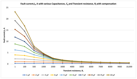
Figure 13.
Fault current, If, A, and transient resistance, Rf for compensated neutral with compensation at 10 kV with the time step of 0.001 s.
Table 15 shows the SPGF current, If, A, and transient resistance, Rf for compensated neutral with overcompensation
Table 15.
SPGF current, If, A, and transient resistance, Rf for compensated neutral, 1.1 overcompensated ASR tuning.
Figure 14 displays SPGF for the compensated neutral system with the ASR set overcompensated. The analysis was made at 10 kV with the simulation time step of 0.001 s. The ZS current falls steadily as the resistance increases. The largest drop is from a few Ohms up to ~2–3 kOhm; beyond that the values are small and flatten. At low resistance, current rises with capacitance; as resistance moves into the hundreds of Ohms to a few kOhm, that dependence weakens; at high resistance (several kOhm) the values for all capacitances cluster to similar small numbers. Compared to the isolated neutral: currents are much lower at the low/medium resistances. Compared to the tuning (1.0 ASR), over-compensation yields slightly higher currents, but the high-resistance tail still matches the same small values as all modes.
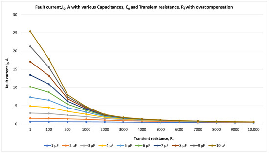
Figure 14.
Fault current, If, A, and transient resistance, Rf for compensated neutral with overcompensation at 10 kV with the time step of 0.001 s.
Table 16 displays the SPGF current, If, A, and transient resistance, Rf for resistively grounded neutral, RN = 100 Ohm.
Table 16.
SPGF current, If, A, and transient resistance, Rf for resistively grounded neutral, NGR RN = 100 Ohm.
Figure 15 shows SPGF for the resistively grounded neutral, and RN = 100 Ohm. The analysis was made at 10 kV with the simulation time step of 0.001 s. The ZS current is very high at the low transient resistance, , and falls steadily as rises. The largest drop occurs from a few Ohms up to a few kOhms; beyond ~3–5 kOhms the values are small and flatten.
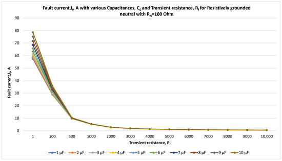
Figure 15.
Fault current, If, A, and transient resistance, Rf for resistively grounded neutral with RN = 100 Ohm at 10 kV with the time step of 0.001 s.
At the low transient resistance, the current increases with capacitance. As transient resistance, reaches hundreds of Ohms to a few kOhms, the dependence on capacitance weakens. At the high transient resistance, (≥~5 kOhms), values across all capacitances converge to nearly the same small numbers. Compared to the isolated neutral, the low transient resistance, currents are an order of magnitude higher, which makes overcurrent pickup much easier. At the high transient resistance, , all modes converge to the same small currents, so the advantage diminishes above several kOhms. Compared with compensated neutrals (ASR 0.9/1.0/1.1), RN = 500 Ohm yields significantly higher currents at low–mid resistances; at high resistances they all converge to the same small band.
Table 17 shows SPGF current, If, A, and transient resistance, Rf for resistively grounded neutral, RN = 500 Ohm.
Table 17.
SPGF current, If, A, and transient resistance, Rf for resistively grounded neutral, NGR RN = 500 Ohm.
Figure 16 shows SPGF for the resistively grounded neutral, RN = 500 Ohm. The analysis was made at 10 kV with the simulation time step of 0.001 s. The ZS current is highest at very low resistance and falls steadily as the transient resistance increases. The biggest drop occurs from a few Ohms up to a few kilohms; beyond ~3–5 kOhm the numbers are small and flatten.
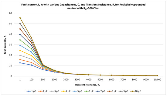
Figure 16.
Fault current, If, A, and transient resistance, Rf for resistively grounded neutral with RN = 500 Ohm at 10 kV with the time step of 0.001 s.
At the low transient resistance, the ZS current rises with capacitance. As the transient resistance reaches hundreds of ohms to a few kOhm, the dependence on capacitance weakens. At the high resistance ≥~5 kOhm, entries for all capacitances converge to nearly the same small numbers.
Compared with RN = 100 Ohm, currents here are much lower at low resistance, but both approaches look similar by ~1 kOhms and beyond. Compared with isolated neutral, RN = 500 Ohm still gives higher currents at very low resistance, but the gap narrows around 1 kOhm and disappears in the multi-kOhm range. Compared with compensated neutrals (ASR 0.9/1.0/1.1), RN = 500 Ohm yields significantly higher currents at low–mid resistances; at high resistances they all converge to the same small band.
Table 18 displays the SPGF current, If, A, and transient resistance, Rf for resistively grounded neutral, NGR RN = 1000 Ohm.
Table 18.
SPGF current, If, A, and transient resistance, Rf for resistively grounded neutral, NGR RN = 1000 Ohm.
Figure 17 shows SPGF for the resistively grounded neutral, RN = 1000 Ohm. The analysis was made at 10 kV with the simulation time step of 0.001 s. The ZS current is highest at very low resistance and falls steadily as resistance increases. The steepest decline is from a few Ohms up to a few kilohms; beyond ~3–5 kOhm the values are small and flatten. At the low transient resistance, the ZS current rises with capacitance. Around 1 kOhm, there is a dependence on capacitance. At the high transient resistance, entries for all capacitances converge to nearly the same small numbers. Compared to the resistively grounded neutral RN = 100 Ohm and RN = 500 Ohm, the RN = 1000 Ohm case yields lower currents at low and mid resistances, but by the multi-kOhm range all three look alike. Compared to the isolated and compensated neutrals, RN = 1000 Ohm still provides higher low-resistance currents but converges to the same small values at the high transient resistance.
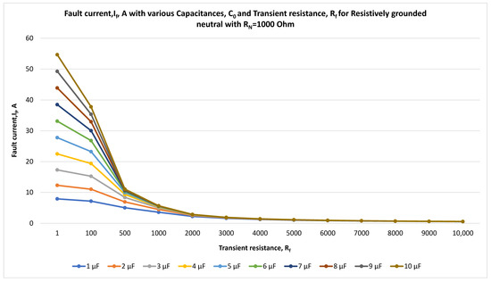
Figure 17.
Fault current, If, A, and transient resistance, Rf for resistively grounded neutral with RN = 1000 Ohm at 10 kV with the time step of 0.001 s.
Our proposed protection device is selective and universal and sustainable, reliable during SPGFs with various transient resistances. Figure 18 displays the disturbance record of CGFPU operation during SPGF for the compensated network. The analyses were made at 10 kV with the simulation time step of 0.001 s. It shows that the CGFPU operates reliably and clears the SPGF in the network with the compensated neutral. There is a sheer angle difference of 180° between the SPGF current of the faulty feeder and capacitive currents of the unfaulted feeders.
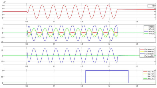
Figure 18.
CGFPU operation during SPGF for compensated network at 10 kV with the time step of 0.001 s.
Figure 19 shows the disturbance record of CGFPU operation during SPGF for a resistively grounded network. It displays the CGFPU detects and operates for the SPGF in the network with the resistively grounded neutral. As there is the active component in the neutral, the angles will differ 120° between the SPGF current of the faulty feeder and capacitive currents of the unfaulted feeders.
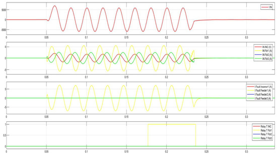
Figure 19.
CGFPU operation during SPGF for resistively grounded network at 10 kV with the time step of 0.001 s.
Therefore, all of this demonstrates that the CGFPU is universal and can be applied in different grounding modes.
5. Development of Algorithm and Protective Device for Identifying a Faulty Feeder During SPGF with the Transient Resistance
A new method for identifying a faulty feeder during a SPGF with the transient resistance is proposed. The method is based on the application of a Centralized Ground Fault Protection Unit (CGFPU), which functions as a digital protective device for centralized monitoring, analysis, and control of the medium-voltage (MV) distribution network. The CGFPU enhances the selectivity and speed of fault detection under conditions where transient resistance significantly complicates feeder identification. Unlike conventional decentralized protection systems, the CGFPU collects, synchronizes, and processes zero-sequence current information from all feeders in real time, enabling accurate determination of the faulty line even in complex fault scenarios. The proposed protective device performs the following essential tasks:
- Angle and magnitude comparison of zero-sequence currents to detect characteristic deviations caused by SPGF occurrence;
- Faulty feeder identification through analysis of deviation patterns between the pre-fault (normal) and post-fault (abnormal) states;
- Decision-making by generating alarm or trip signals depending on the severity, persistence, and confirmation of the ground fault condition.
The overall configuration of the protective system is illustrated in Figure 20, which presents the functional diagram of the centralized ground fault protection unit in a 10 kV distribution network with isolated neutral. The diagram shows the interconnection between measurement units, synchronization modules, digital processing blocks, and the fault decision logic.
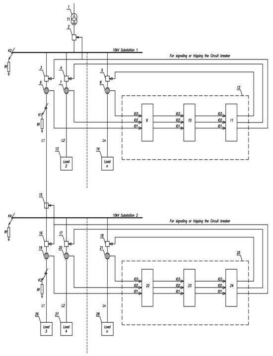
Figure 20.
Functional diagram of the CGFPU in the 10 kV network with the isolated neutral configuration.
The structure of the proposed centralized protection system is presented in Figure 20. The main components of the system are: 1—power transformer; 2—incomer circuit breaker in Substation No.1; 3, 4, 5—circuit breakers of outgoing feeders in Substation No.1; 6, 7, 8—zero-sequence current transformers (ZCTs) of the outgoing feeders in Substation No.1; 9—angle comparison module in Substation No.1; 10—magnitude comparison module in Substation No.1; 11—output module in Substation No.1; 12—centralized ground fault protection unit in Substation No.1; 13, 14—loads supplied by in Substation No.1; 15—incomer circuit breaker in Substation No.2; 16, 17, 18—circuit breakers of outgoing feeders in Substation No.2; 19, 20, 21—zero-sequence current transformers of the outgoing feeders in Substation No.2; 22—angle comparison module in Substation No.2; 23—magnitude comparison module in Substation No.2; 24—output module in Substation No.2; 25—centralized ground fault protection unit in Substation No.2; 26, 27, 28—loads supplied by Substation No.2.
Zero-sequence currents from each feeder are continuously measured by ZCTs (6–8, 19–21). These currents are fed into the angle comparison and magnitude comparison modules (blocks 9, 10, 22, 23), and the processed results are sent to the output modules (blocks 11, 24), which generate the final control signals.
Normal (Fault-Free) Operating Mode: During normal operation of the 10 kV isolated neutral network, imbalance currents or charging currents may occur. The operation proceeds as follows:
- -
- If the measured zero-sequence current I0 from ZCTs exceeds the preset alarm or trip thresholds, the signals are transmitted to the angle comparison modules (blocks nine, twenty two).
- -
- In this state, the phasors of zero-sequence currents across all feeders are approximately aligned in the same direction and have small magnitudes.
- -
- No significant angle deviations or overcurrent conditions are detected.
- -
- Consequently, the output modules (blocks 11, 24) do not issue an alarm or trip command.
This logic ensures that the CGFPU eliminates false trips caused by charging or imbalance currents during fault-free conditions.
When an SPGF with the transient resistance occurs, a distinct pattern of zero-sequence currents emerges:
- Fault signal formation
- -
- A zero-sequence current appears on the faulty line.
- -
- Capacitive currents from the unfaulted lines also flow, producing measurable zero-sequence components.
- Angle comparison
- -
- In the angle comparison modules (blocks nine, twenty two), phasors of the zero-sequence currents are analyzed.
- -
- The faulty line’s current phasor exhibits an approximately 180° phase shift relative to the capacitive current phasors of the unfaulted lines.
- Magnitude comparison
- -
- In the magnitude comparison modules (blocks 10, 23), the absolute values of zero-sequence currents are compared.
- -
- The feeder with the maximum magnitude is selected as the most probable faulty feeder.
- Decision-making
- -
- In the output modules (blocks 11, 24), the faulty feeder is definitively identified.
- -
- An alarm signal depending on the SPGF transient resistance is issued for operator’s attention, or if there is a bolted SPGF and the setting value is exceeded, a trip command is sent to the corresponding circuit breaker, isolating the faulty feeder or a bus.
If the SPGF occurs on the first outgoing line L1 at point K1 (Figure 20), the zero-sequence current phasor L1 of the faulty line will be directed opposite (≈180° phase shift) to the capacitive current phasors IL2, IL3,…, ILn of the unfaulted lines.
This relation is shown in Figure 21, which presents the phasor diagram of zero-sequence currents during SPGF at line L1. The phase opposition between the faulty feeder current and the unfaulted feeders’ capacitive currents serves as a reliable indicator for fault identification.
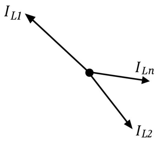
Figure 21.
Phasor diagram of the ground fault current and capacitive currents during a ground fault on an outgoing feeder.
Feeder fault (point K1, Figure 21): When SPGF occurs on an outgoing feeder, the faulty line’s zero-sequence current phasor is directed approximately 180° opposite to the phasors of the unfaulted feeders’ capacitive currents. The unfaulted feeders’ phasors are relatively aligned, forming a compact angular grouping. This clear phase opposition is the main indicator used by the CGFPU to distinguish the faulty feeder from the unfaulted ones.
Busbar fault (point K2, Figure 22): If SPGF occurs on the substation busbars, all outgoing feeders’ zero-sequence current phasors (IL1, IL2, …, ILn) are directed in the same direction. These phasors represent only the feeders’ capacitive currents relative to ground. In this case, there is no 180° opposition, which allows the CGFPU to recognize the fault location as being on the busbars rather than on a specific feeder.
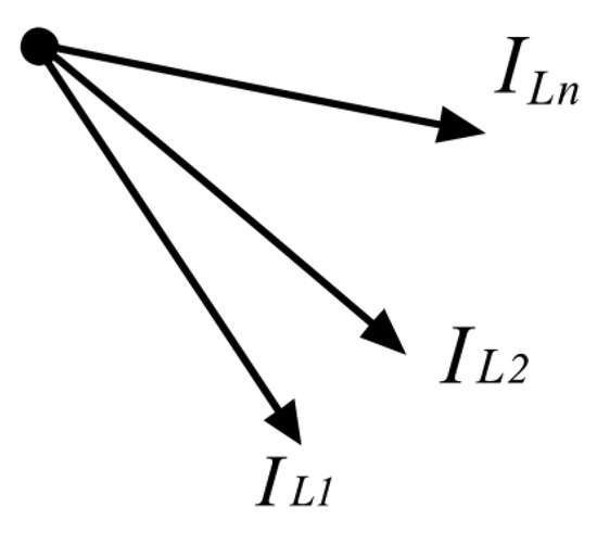
Figure 22.
Phasor diagram of zero-sequence currents during ground fault on the 10 kV busbars.
5.1. Description of Centralized Ground Fault Protection Unit
Based on the functional diagram in Figure 20, a protection scheme has been developed using zero-sequence current (ZSC) angle and magnitude comparison.
During an SPGF, ZSC signals are transmitted.
From the ZSCTs of Feeders No.1, 2, and 3 in Substation No.1 (TR1 10 kV CT1 SS1, Feeder 1–3 CT1 SS1) to the CGFPU (Centralized Ground Fault Protection 10 kV SS1). From the ZSCTs of Feeders No.1, 2, and 3 in Substation No.2 (INC 10 kV CT1 SS2, Feeder 1–3 CT1 SS2) to the CGFPU (Centralized Ground Fault Protection 10 kV SS2). The block diagrams of the CGFPU in the 10 kV isolated neutral network of Substations No.1 and No.2 are shown in Figure 23 and Figure 24.
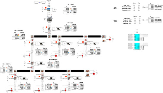
Figure 23.
Single-line diagram of a 110/10 kV Substation in the network with the isolated neutral configuration.
Figure 24.
Block diagram of the CGFPU in a 10 kV network with the isolated neutral configuration for the Substations No.1 and No.2.
If a circuit breaker is in service, its auxiliary contact is closed, and the feeder ZSC signal participates in the protection logic. If the breaker trips or is out of service, the corresponding feeder is removed from the scheme, and the switch output is set to logical zero (Figure 25).
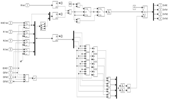
Figure 25.
Functional diagram of the CGFPU polarization module in the 10 kV network with the isolated neutral configuration for the Substation No.1 and No.2.
ZSC signals enter the polarization module. Signals pass through switches and are forwarded to the “Magnitude–Angle to Complex” converter and then to the angle summation block. The total number of active breakers is taken into account; the average phasor angle of unfaulted feeders is calculated.
The ZSC phasor of each feeder is compared with the average angle of the unfaulted feeders. If the phase difference satisfies: Δφ = 1800 ± 20%, then a logical “1” is generated at the output of the OR operator. The signal proceeds to the multiport switch for further processing.
Among the feeders, the ZSC with the maximum magnitude is selected (Figure 26). This signal is forwarded to the AND operator. If both conditions are satisfied—(i) magnitude exceeds the threshold and (ii) phase opposition ≈ 180°—then the AND operator outputs logical “1”.
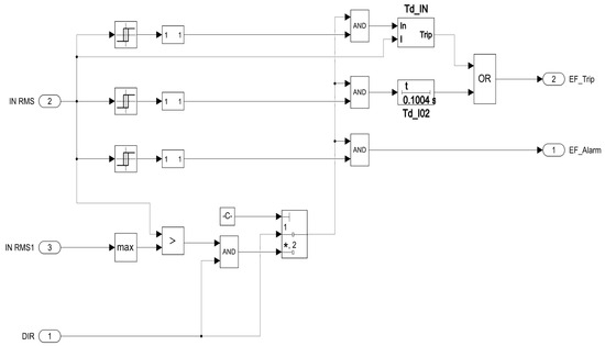
Figure 26.
Functional diagram of the angle and magnitude comparison module for Feeders No.1, 2, and 3 in the Substations No.1 and No.2.
If the alarm setting is exceeded, then an SPGF signal will appear. If the trip setting is exceeded, then the operate delay time of the Feeder No.1, in Substation No.1, will be 300 ms, and for the remaining feeders, Substations No.1 and No.2, it will be 100 ms and a trip signal of the corresponding feeder will turn up.
5.2. Algorithm of CGFPU Operation During Bus Ground Faults
When SPGF occurs on the substation busbars, the following conditions are observed (see Figure 27). The zero ZSC reaches a maximum value due to the summation of all feeders’ capacitive currents. The resulting ZSC signal is directed at the Magnitude Comparison Module. If the alarm setting is exceeded, an SPGF alarm signal is issued. If the trip setting is exceeded, a trip signal is generated after a 100 ms intentional delay, opening the incomer circuit breaker of the affected substation.
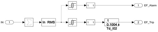
Figure 27.
Functional diagram of the magnitude and angle comparison module for the incomers in substations No.1 and No.2.
To ensure stable relay performance under signal noise, arcing faults, or transient switching events, the CGFPU employs the following techniques:
- Zero-sequence currents are filtered over several cycles (typically 40–60 ms) to suppress high-frequency noise and transient disturbances;
- A phase difference of at least 200° < ∣Δφ∣ > 160° must exist between the fault current and the unfaulted feeders’ capacitive currents to confirm a ground fault;
- To prevent false tripping due to short-lived events (e.g., noise, momentary saturation, extinguishing arc faults), the CGFPU requires fault confirmation across multiple consecutive cycles;
- Specifically, at least three out of five half-cycles must indicate valid fault conditions, persisting for ≥two to three cycles before operation is permitted;
- Based on this rule, a minimum delay of td = 100 ms is introduced.
During single pulse and intermittent arcing ground faults with the high transient resistance, which will be accompanied with overvoltages (Figure 28 and Figure 29) that will drop significantly during the current crossing zero, the CGFPU will issue an alarm (Figure 28) and the duty personnel will be informed of the ground fault inception. As the ground fault start persisting and will last for at least 100 ms and the ground fault current will reach the ground overcurrent setting, the CGFPU will issue a trip signal and isolate the faulty feeder (Figure 29). This proves that the proposed method is stable and efficient during single pulse and intermittent arcing ground faults.
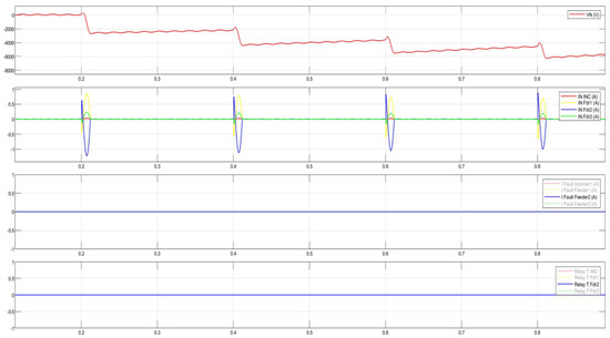
Figure 28.
Disturbance record of the CGFPU issuing an alarm for single pulse arcing SPGF at 10 kV.
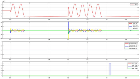
Figure 29.
Disturbance record of the CGFPU issuing a trip signal during intermittent arcing SPGFs at 10 kV.
5.3. CGFPU Flowchart Diagram
1. Start for Faulty Feeder or Busbar Fault Identification.
This step initiates the fault identification process when an abnormal condition is suspected on a feeder connected to a busbar. The system monitors the zero-sequence currents for indications of SPGF (Figure 30)
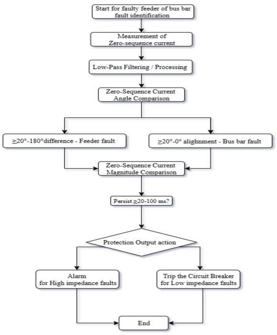
Figure 30.
Flow diagram of the CGFPU.
Objective: Determine whether the fault lies on the feeder or the busbar.
2. Measurement of Zero-Sequence Current
The zero-sequence current (I0) is the sum of the three-phase currents:
This component is typically negligible under balanced conditions but becomes significant during ground faults.
- ZSCTs are used for this measurement.
- Essential for sensitive ground fault detection.
3. Low-Pass Filtering/Signal Processing
Zero-sequence current signals often contain noise and transient components.
- A low-pass filter removes high-frequency noise and harmonics.
- Ensures accurate angle and magnitude comparison.
- Helps in preventing false trips due to switching transients or noise.
4. Zero-Sequence Current Angle Comparison
This is a critical decision point where the phase angle of the zero-sequence current from each feeder is compared with the reference (busbar or neutral current).
If angle difference ≥20° to 180° → Feeder fault
- It indicates that the current is out of phase with the busbar’s zero-sequence current.
- It suggests that the fault lies beyond the ZSCTs, on the feeder.
If angle difference ≤20°—Busbar fault
- It indicates that the zero-sequence currents are in phase or closely aligned.
- It suggests a fault located within the protection zone, i.e., busbar zone.
5. Zero-Sequence Current Magnitude Comparison
This step validates the angle comparison by evaluating the magnitude of the zero-sequence current.
- Large magnitude = low impedance fault
- Small magnitude = high impedance fault
This check ensures that even high-resistance faults which might have low current magnitude are detected properly.
6. Time Persistence Check (≥20–100 ms)
A stability time delay ensures the fault condition is not transient.
- Short-duration spikes or oscillations are ignored.
- Prevents unnecessary tripping due to momentary disturbances.
- The delay (20–100 ms) is selected based on the following:
- System dynamics;
- Speed of protective relays;
- Fault clearing time.
7. Protection Output Action
Based on the magnitude and persistence of the fault, the system initiates one of two actions:
(a) Alarm for High-Impedance Faults
- If fault current is small suggesting a high-impedance fault, only an alarm is issued.
- Allows for manual inspection or further diagnostic steps.
- Prevents unnecessary power disruption for non-critical faults.
(b) Trip Circuit Breaker for Low Impedance Faults
- If the fault current is large and persistent indicative of a serious SPGF, the associated circuit breaker is tripped.
- Ensures fast isolation of the faulted section.
- Protects equipment and maintains system stability and safety.
8. End
The flow ends once the protection logic has either:
- Issued an alarm, or
- Tripped the circuit breaker and isolated the fault.
The system now waits for the duty electrical operator or automation to reset the logic or reclose the breaker.
5.4. Practical Implementation Challenges of the CGFPU
Although the proposed CGFPU is conceptually robust and validated through modeling, several practical aspects must be considered before field application.
1. Communication Requirements Between Feeders
Unlike schemes that rely on digital protocols (IEC 61850 GOOSE/SV, synchrophasors, or GPS-based phasor alignment), the CGFPU can operate in a copper-wired configuration.
- Zero sequence currents (3I0): Each feeder provides a ZS current signal from a zero-sequence CT (core-balance or Holmgreen connection). These are directly wired to the central unit.
- No special protocols: This eliminates the need for time synchronization or substation LAN bandwidth. Signals are transmitted continuously and deterministically.
- Wiring considerations: The drawback is increased cabling volume. For eight to twelve feeders, each 3I0 signal requires a dedicated pair of wires. CT secondary burden and distance must be managed to avoid distortion.
2. Sampling Rate and Signal Processing
Since the CGFPU makes its decision based on the phasor relationships of feeder ZS currents, the processing requirements are modest.
- Sampling frequency: 1–2 kHz (20–40 samples per cycle) is sufficient for fundamental-frequency phasors. For higher fidelity and transient discrimination, ≥4 kHz is recommended.
- Phasor estimation: A one-cycle discrete Fourier transform with a sliding window provides accurate magnitude and angle estimation with minimal delay.
- Filtering: Digital low-pass or notch filters are required to mitigate noise and suppress harmonics, especially in networks with inverter-based generation.
- Latency: Operating time remains within 20–40 ms (one to two cycles), meeting distribution network protection speed requirements.
3. Hardware Constraints
- Central CGFPU unit: Requires multiple analog input channels (one per feeder), rated for 1 A CT secondary signals.
- Burden management: Each ZSCT circuit must be sized so that the additional wiring to the CGFPU does not exceed the ZSCT’s rated burden.
- Reliability: The CGFPU is a single point of failure. To meet utility protection standards, redundant units (primary + hot-standby) should be installed, both fed from the same ZSCT circuits.
4. Compatibility with Existing Protection Infrastructure
- Parallel operation: The CGFPU acts as a supervisory selective protection. Existing feeder relays—directional ground fault, overcurrent protections remain in service as backup.
- Fallback protection: In case the CGFPU is unavailable (failure, maintenance, wiring issue), feeder relays continue to provide non-selective or delayed fault clearing.
- Integration path: The scheme can be retrofitted into conventional substations without replacing feeder relays, requiring only additional CT wiring to the central unit.
- Scalability: The approach is effective for small and medium substations (four to twelve feeders). For very large busbars, scalability may become constrained by wiring bulk and input channel limits.
5. Deployment Challenges and Mitigation
- Cabling complexity: Mitigated by structured wiring harnesses or installing the CGFPU close to the MV switchgear.
6. Results
We will calculate SPGF for different transient resistances, analyze and evaluate the obtained values and calculate the CGFPU settings at Rf = 5000 Ohm at the Feeder No.1, Substation No.1 bus and at the Feeder No.1, Substation No.2 bus. The SPGF calculation and analysis of ground fault protection were performed on sections of the 10 kV distribution network at the Substations No.1 and 2, and the single line diagram is shown in the Figure 31.
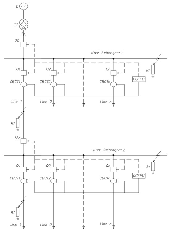
Figure 31.
10 kV distribution network with the isolated neutral configuration.
Power supply: Short-circuit power Ssc = 40 MVA, voltage: U = 110 kV, ratio of reactive resistance to active resistance: X/R = 7, high voltage neutral mode network with the solidly grounded neutral configuration.
Power transformer: transformer type is TM-60000/110/10; apparent power S = 60 MVA; voltage on the primary winding: U1 = 110 kV; voltage on the secondary winding: U2 = 10 kV; transformation ratio Ktr = 11; primary current I1 = 314.9 A; I2 = 3464.2 A, vector group Yn/D–11; short-circuit voltage: Usc = 20%; medium voltage neutral mode isolated neutral configuration; resistance R1 = 0.002 p.u, R2 = 0.002 p.u; inductance L1 = 0.1 p.u; L2 = 0.1 p.u, magnetizing resistance Rm = 3631 p.u; magnetizing inductance: Lm = 4021 p.u; zero-sequence flux inductance L0 = 0.5 p.u.
Substation No.1
Feeder 1: cable cross-section, S = 240 mm2, number of cores n = 3, voltage U1 = 6/10 kV, nominal current Inom = 405 A, short-circuit current Isc = 22.9 kA, impedance Z = 0.0158 + j0.0758 Ω/km, positive-sequence inductance L1 = 0.301 × 10⁻³ H/km, zero-sequence inductance L0 = 0.903 × 10⁻³ H/km, positive-sequence capacitance C1 = 0.440 × 10⁻⁶ μF/km, zero-sequence capacitance C0 = 0.440 × 10⁻⁶ μF/k, length l = 1 km.
Feeder 2: cable cross-section, S = 240 mm2, number of cores n = 3, voltage U1 = 6/10 kV, nominal current Inom = 405 A, short-circuit current Isc = 22.9 kA, impedance Z = 0.0158 + j0.0758 Ω/km, positive-sequence inductance L1 = 0.301 × 10⁻³ H/km, zero-sequence inductance L0 = 0.903 × 10⁻³ H/km, positive-sequence capacitance C1 = 0.440 × 10⁻⁶ μF/km, zero-sequence capacitance C0 = 0.440 × 10⁻⁶ μF/k, length l = 1.2 km.
Feeder 3: cable cross-section, S = 240 mm2, number of cores n = 3, voltage U1 = 6/10 kV, nominal current Inom = 405 A, short-circuit current Isc = 22.9 kA, impedance Z = 0.0158 + j0.0758 Ω/km, positive-sequence inductance L1 = 0.301 × 10⁻³ H/km, zero-sequence inductance L0 = 0.903 × 10⁻³ H/km, positive-sequence capacitance C1 = 0.440 × 10⁻⁶ μF/km, zero-sequence capacitance C0 = 0.440 × 10⁻⁶ μF/k, length l = 1.1 km.
Load 1, 2, 3: power consumption P = 7 MW, reactive power Q = 2 MVAr, nominal current Inom =405 A, power factor cosφ = 0.86, nominal voltage U = 10 kV.
Substation No.2
Feeder 1: cable cross-section, S = 240 mm2, number of cores n = 3, voltage U1 = 6/10 kV, nominal current Inom = 405 A, short-circuit current Isc = 22.9 kA, impedance Z = 0.0158 + j0.0758 Ω/km, positive-sequence inductance L1 = 0.301 × 10⁻³ H/km, zero-sequence inductance L0 = 0.903 × 10⁻³ H/km, positive-sequence capacitance C1 = 0.440 × 10⁻⁶ μF/km, zero-sequence capacitance C0 = 0.440 × 10⁻⁶ μF/k, length l = 1.6 km.
Feeder 2: cable cross-section, S = 240 mm2, number of cores n = 3, voltage U1 = 6/10 kV, nominal current: Inom = 405 A, short-circuit current Isc = 22.9 kA, impedance Z = 0.0158 + j0.0758 Ω/km, positive-sequence inductance L1 = 0.301 × 10⁻³ H/km, zero-sequence inductance L0 = 0.903 × 10⁻³ H/km, positive-sequence capacitance C1 = 0.440 × 10⁻⁶ μF/km, zero-sequence capacitance C0 = 0.440 × 10⁻⁶ μF/k, length l = 0.9 km.
Feeder 3: cable cross-section, S = 240 mm2, number of cores n = 3, voltage U1 = 6/10 kV, nominal current Inom = 405 A, short-circuit current Isc = 22.9 kA, impedance Z = 0.0158 + j0.0758 Ω/km, positive-sequence inductance L1 = 0.301 × 10⁻³ H/km, zero-sequence inductance L0 = 0.903 × 10⁻³ H/km, positive-sequence capacitance C1 = 0.440 × 10⁻⁶ μF/km, zero-sequence capacitance C0 = 0.440 × 10⁻⁶ μF/k, length l = 0.9 km.
Load 1, 2, 3: power consumption P = 7 MW, reactive power Q = 2 MVAr, nominal current Inom = 405 A, power factor cosφ = 0.86, nominal voltage U = 10 kV.
To analyze characteristics of changes in the SPGF currents and capacitive currents for different values of the transient resistances, it is required to evaluate the magnitude of the ground fault current flowing in the fault location, the zero-sequence voltage and the coefficient of ground fault incompleteness, which are determined by the following expressions:
6.1. Analysis of SPGF Current with Different Transient Resistances at the Feeder No.1, Substation No.1 in the 10 kV Network with the Isolated Neutral Configuration
Figure 31 shows the single line diagram of 10 kV distribution network with the isolated neutral configuration.
Table 19 shows the SPGF values with the different transient resistances at the Feeder No.1, Substation No.1.
Table 19.
SPGF current values at the Feeder No.1, Substation No.1 for different transient resistances and capacitive currents in the 10 kV network with the isolated neutral configuration.
Table 20 shows dependence of the circuit completeness, sensitivity ratio, zero-sequence voltage and current angle difference from transient resistances during single-phase ground fault at the Feeder No.1, Substation No.1.
Table 20.
Dependence of the Loop integrity coefficient, sensitivity ratio, zero-sequence voltage and current angle difference from transient resistances during SPGF at the Feeder No.1, Substation No.1.
Figure 32 shows the change in the SPGF current and capacitive currents with the different transient resistances in the range of 1 Ohm to 10,000 Ohm at the Feeder No.1, Substation No.1. The total cumulative current at the fault location (brown curve) is at its highest magnitude at Rf = 1 Ohm, Igf = 15.82 A and decreases sharply with increasing resistance and reaches the lowest point at Rf = 10,000 Ohm, Igf = 0.54 A.
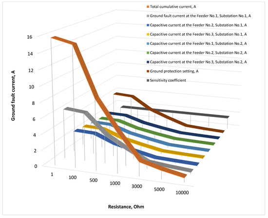
Figure 32.
Total cumulative current, sensitivity ratio, ground fault current with transient resistances at the Feeder No.1, Substation No.1, and capacitive currents in the 10 kV network with the isolated neutral configuration.
The ground fault current seen by the relay (grey curve) at the Feeder No.1, Subststaion 1 is at its maximum value at Rf = 1 Ohm, If = 6.37 A and drastically decreases with an increase in transient resistances and drops at Rf = 10,000 Ohm, If = 0.22 A. As it can be noticed, the sensitivity ratio is 1.5 from Rf = 1 to Rf = 10,000 Ohm, and is characterized with a steady state behavior, which proves the efficiency of the proposed device, specifically the CGFPU. The zero-sequence currents have a conspicuously expressed angle difference which serves as a good and effective polarization signal.
Figure 33 shows the change in the zero-sequence voltage during the SPGF with the different transient resistances in the range of 1 Ohm to 10,000 Ohm at the Feeder No.1, Substation No.1.
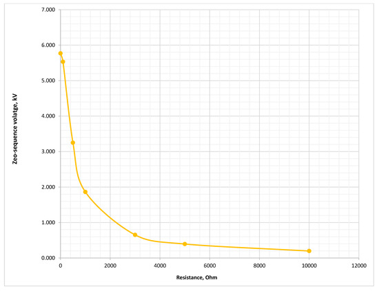
Figure 33.
Zero-sequence voltage during SPGF with transient resistances at the Feeder No.1, Substation No.1 in the 10 kV network with the isolated neutral configuration.
It can be noted that during the metallic ground fault, Rf =1–100 Ohm, there is a significant neutral voltage displacement, and the zero-sequence voltage equals the neutral voltage reaches the values of 5.77–5.532 kV. At the transient resistance of Rf = 500–3000 Ohm, the zero-sequence voltage reaches 3.25–0.653 kV. At the high transient resistance Rf = 5000–10,000 Ohm, the zero-sequence voltage goes down from 0.394 to 0.197 kV. The neutral point shift is at its lowest point.
Figure 34 illustrates the variation of the angular difference between the zero-sequence current of the faulted feeder and those of the unfaulted feeders as a function of the fault resistance Rf. At the low resistance values Rf = 1–100 Ohm, the fault current is relatively high, and the angle difference is exactly 180°. This indicates distinct phase-opposition between the faulted feeder’s current and the vector sum of the unfaulted feeders’ capacitive currents.
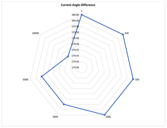
Figure 34.
Current angle difference during SPGF with transient resistance at the Feeder No.1, Substation No.1 in the 10 kV network with the isolated neutral configuration.
Such behavior is consistent with theoretical expectations for SPGFs in isolated networks, where the ZSC is almost purely resistive and directly counteracts the system’s capacitive current.
At the medium resistance values Rf = 500–3000 Ohm, the fault current magnitude decreases due to the higher fault resistance. The angular difference slightly reduces to approximately 179.98–179.97°, yet the current remains nearly in anti-phase, preserving a clear directional distinction. At the high resistance values Rf = 5000–10,000 Ohm, the fault current diminishes further, approaching the magnitude of the capacitive current. The angular difference remains stable at around 179.97°, still well separated from the angles of the healthy feeders. The total deviation across four orders of magnitude in fault resistance is only about 0.04°, which highlights the robustness of angle-based discrimination. This behavior confirms that the faulted feeder can be reliably identified based on angular criteria, even under very high fault resistances where the zero-sequence current magnitude is minimal.
Figure 35 presents the variation of the loop integrity coefficient, β with respect to the transient resistance Rf. This coefficient reflects the fault’s ability to establish a return path for the zero-sequence current, thereby indicating the degree of neutral point displacement and the overall severity of the ground fault.
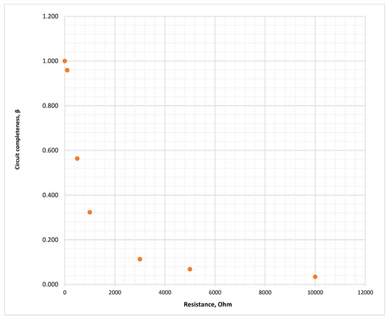
Figure 35.
Loop integrity coefficient during SPGF with transient resistances at Feeder No.1, Substation No.1 in the 10 kV isolated neutral network.
At very low resistance values Rf − 1 Ohm, the loop integrity coefficient approaches unity β − 1, which corresponds to a metallic or bolted ground fault condition. In this case, the ground path is solid, the fault current reaches its maximum, and the neutral point is strongly displaced. For Rf = 1–100 Ohm, the loop integrity coefficient decreases slightly from β = 1 to 0.959, indicating that the system still experiences a severe ground fault with a clear return path for the zero-sequence current.
At the medium resistance values Rf = 500–3000 Ohm, the loop integrity coefficient progressively decreases to β = 0.563–0.113. This reduction signifies that the SPGF current weakens with increasing resistance, leading to a reduced ability to shift the neutral potential. The severity of the SPGF diminishes, and detection becomes more challenging.
At the high resistance values Rf = 5000–10,000 Ohm, the c loop integrity coefficient falls further to β = 0.063–0.034. In this range, the ground fault current is minimal, and the neutral point shift is weak. Such high-resistance faults pose a challenge for detection, as the loop integrity completeness is low and the fault magnitude is almost negligible.
Overall, the behavior of the loop integrity coefficient β highlights its usefulness as a diagnostic parameter for assessing fault severity and the ability of the ground fault to displace the neutral potential across different resistance levels.
Figure 36 illustrates the phasor relationships between the SPGF current at the faulty feeder and the capacitive currents of the unfaulted feeders. The fault current remains almost in phase opposition (∠180°) with the sum of the unfaulted feeders’ capacitive currents, which is consistent with the behavior of SPGFs in isolated neutral systems.
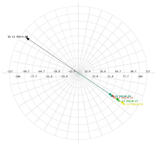
Figure 36.
Phasor diagram for SPGF at the Feeder No.1, Substation No.1 and capacitive currents in the 10 kV network with the isolated neutral configuration.
In the case of a bolted SPGF Rf ≈ 1 Ohm, the SPGF current reaches its maximum value of approximately 10–16 A. In contrast, when the transient resistance reaches its maximum level Rf = 10,000 Ohm, the SPGF current drops to fractions of an ampere (tenths of an ampere). This wide variation confirms the strong dependence of SPGF current magnitude on transient resistance, while the phasor angle relation remains nearly constant.
6.2. Analysis of Single-Phase Ground Fault Current with Different Transient Resistances on the Substation No.1 Bus in the 10 kV Network with the Isolated Neutral Configuration
Table 21 presents the calculated ground fault currents for various values of transient resistance Rf, along with the capacitive currents of each feeder.
Table 21.
SPGF current values with different transient resistances on the Substation No.1 bus and capacitive currents in the 10 kV network with the isolated neutral configuration.
- -
- At the low resistances Rf = 1–100 Ohm, the cumulative SPGF current is high≈ 15–16 A and clearly exceeds the capacitive currents of the unfaulted feeders. The phasor angles confirm a nearly 180° phase opposition.
- -
- At the medium resistances Rf = 500–3000 Ohm, the SPGF current decreases significantly ≈ 9.02 A–1.81 A, yet it remains distinguishable from background capacitive currents, with the phase angle staying close to 180°.
At the high resistances Rf = 5000–10,000 Ohm, the SPGF current weakens drastically ≈ 1.09 A–0.55 A, approaching the magnitude of individual feeder capacitive currents. Despite the very low current, the phase opposition remains observable, enabling faulted feeder identification.
Table 22 displays dependence of circuit completeness, sensitivity ratio, zero-sequence voltage and current angle difference from transient resistance during single phase ground fault on the Substation No.1 bus.
Table 22.
Dependence of circuit completeness, sensitivity ratio, zero-sequence voltage and current angle difference from transient resistance during single phase ground fault on the Substation No.1 bus.
Figure 37 illustrates the variation of the SPGF current and feeder capacitive currents with different transient resistances in the range of Rf = 1–10,000 Ohm on the Substation No.1 bus. The dependency is distinctly non-linear, reflecting the strong influence of the transient resistance on fault current magnitude. At low resistance values Rf = 1 Ohm, the cumulative SPGF current (yellow curve) reaches its maximum of If = 16.01 A. As the resistance increases, the ground fault current decreases progressively, reaching a minimum value of If = 0.55 A at Rf = 10,000 Ohm.
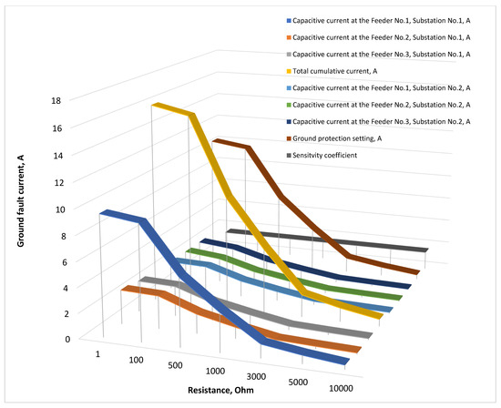
Figure 37.
Ground fault current with the transient resistance on the Substation No.1 bus and capacitive currents in the 10 kV network with the isolated neutral configuration.
The ZS currents of unfaulted feeders correspond to their inherent capacitive currents at low resistance conditions. With the increase in Rf, these currents reduce proportionally, following the same non-linear trend as the fault current.
Importantly, the sensitivity ratio remains constant at 1.5 across the entire resistance range, from Rf = 1 Ohm up to Rf = 10,000 Ohm. This invariability demonstrates the robustness of the proposed CGFPU, ensuring reliable performance even under weak fault conditions characterized by high transient resistance.
Figure 38 presents the variation of zero-sequence voltage under SPGF conditions at the Substation No.1 bus for different transient resistances ranging from Rf = 1 Ohm to Rf = 10,000 Ohm. At the low transient resistances Rf = 1–100 Ohm, a strong displacement of the neutral point is observed, where the ZSV equals the neutral voltage. The measured values are high, reaching 5.77–5.53 kV, indicative of a metallic or nearly bolted fault condition.
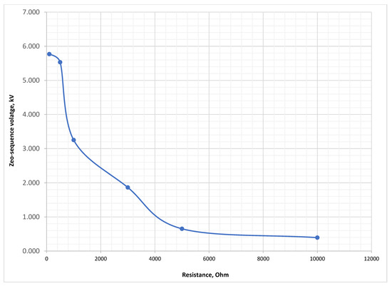
Figure 38.
Zero-sequence voltage during SPGF with transient resistances on the Substation No.1 bus in the 10 kV network with the isolated neutral configuration.
At the medium resistances Rf = 500–3000 Ohm, the zero-sequence voltage (ZSV) decreases to 3.25–0.652 kV. This reflects a weakening of the fault current contribution and a partial reduction in the neutral point displacement.
At the high resistances Rf = 5000–10,000 Ohm, the ZSV further drops to 0.393–0.198 kV, indicating that the neutral point shift becomes minimal and the fault is weak in terms of measurable impact.
Figure 39 depicts the behavior of the angular difference between zero-sequence currents of unfaulted feeders during SPGF events at the Substation No.1 bus.
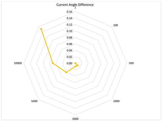
Figure 39.
Current angle difference during SPGF with transient resistances on the Substation No.1 bus in the 10 kV network with the isolated neutral configuration.
- -
- At low resistance values Rf = 1–100 Ohm, the ground fault current is high, and the angular difference approaches 0°, showing that all unfaulted feeders’ currents are aligned in phase. This alignment confirms that the ground fault occurs at the bus bars, producing a uniform current distribution across healthy feeders.
- -
- At medium resistances Rf = 500–3000 Ohm, the ground fault current magnitude decreases due to the resistance increase. The angular difference slightly shifts to about 0.01°, but the currents still preserve a nearly identical phase, allowing accurate directional detection.
At high resistances Rf = 5000–10,000 Ohm, the ground fault current becomes minimal. The angular difference increases modestly to 0.15°, yet the phase relationship between faulty and unfaulted feeders remains sufficiently distinct. This stability demonstrates that the location of the fault can still be reliably identified even under very weak fault conditions.
Figure 40 shows the change in the loop integrity coefficient β with varying transient resistance.
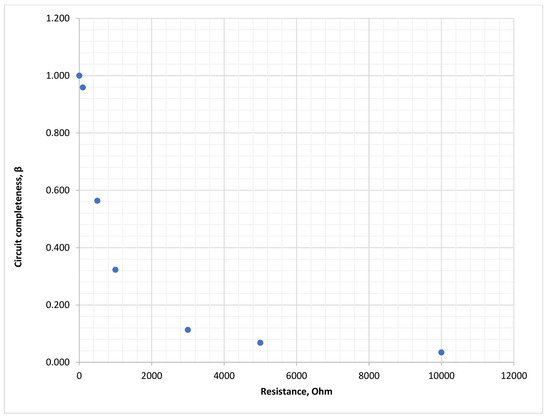
Figure 40.
Loop integrity coefficient during SPGF with transient resistances on the Substation No.1 bus in the 10 kV network with the isolated neutral configuration.
- -
- At the low transient resistances Rf = 1–100 Ohm, the coefficient remains close to unity β = 1–0.959. This condition corresponds to a metallic or bolted fault, where the SPGF current reaches its maximum and the neutral point displacement is significant. The network operates in a nearly complete faulted circuit, and the fault is easily detectable.
- -
- At the medium resistances Rf = 500–3000 Ohm, the loop integrity coefficient decreases progressively to values in the range of β = 0.563–0.113. In this zone, the SPGF current is considerably reduced, and the neutral point displacement weakens. The SPGF transitions from a severe state to a less pronounced one, making detection more challenging but still feasible.
At the high transient resistances Rf = 5000–10,000 Ohm, the coefficient further diminishes to very low values of β = 0.068–0.034. Under these conditions, the SPGF current, capacitive current, and zero-sequence voltage magnitudes all reach their lowest values. The fault severity is minimal, and the neutral point shift is nearly absent. This scenario represents the most difficult case for detection, where highly sensitive protection devices, such as the proposed CGFPU, are essential to ensure fault identification.
Figure 41 illustrates the phasor relationships of currents under SPGF conditions. The capacitive currents are proportional to the capacitances of their respective feeders. Their directions are almost aligned, with only slight angular shifts caused by the network asymmetry. In the case of a bolted SPGF, low transient resistance, the SPGF current reaches values on the order of several tens of amperes. Conversely, when the transient resistance is very high, the SPGF current is significantly reduced, reaching tenths of an ampere. This demonstrates the non-linear dependence of the SPGF current magnitude on the transient resistance.
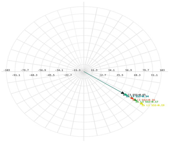
Figure 41.
Phasor diagram for the SPGF on the Substation No.1 bus and capacitive currents in the 10 kV network with the isolated neutral configuration.
6.3. Analysis of Single-Phase Ground Fault Current with Different Transient Resistances at the Feeder No.1, Substation No.2 in the 10 kV Network with the Isolated Neutral Configuration
Table 23 presents detailed current values under SPGF conditions at Feeder No.1, Substation No.2, for various transient resistances ranging from 1 Ohm to 10,000 Ohm. Both cumulative and feeder-specific capacitive currents are provided, along with their corresponding phasor angles.
Table 23.
SPGF current values with different transient resistances at the Feeder No.1, substation No.2, and capacitive currents in the 10 kV network with the isolated neutral configuration.
At the low resistance Rf = 1 Ohm, the cumulative SPGF current is at its maximum 15.72 A∠−130°, dominated by the ground fault component at Feeder No.1 13.49 A∠−130°. As the transient resistance increases, the SPGF current progressively decreases. For example, at Rf = 500 Ohm, the SPGF current is reduced to 7.59 A ∠−174.6°, and at Rf = 10,000 Ohm, it drops further to 0.46 A ∠−142.28°.
The angular characteristics also shift—the capacitive currents of unfaulted feeders are nearly in quadrature to the fault current at the low resistances but gradually converge in phase as resistance increases. This trend confirms the weakening of the neutral point displacement with higher Rf.
Table 24 quantifies the parameters characterizing circuit performance during SPGF.
Table 24.
Dependence of the Loop integrity coefficient, sensitivity ratio, zero-sequence voltage, and current difference from transient resistance during SPGF at the Feeder No.1, Substation No.2.
- -
- Loop integrity coefficient, β: At the low transient resistance Rf = 1–100 Ohm, loop integrity coefficient, β is close to unity 1.00–0.96, indicating strong coupling of the faulted phase to the ground and a significant neutral point displacement. As resistance increases, the loop integrity coefficient decreases sharply, reaching 0.03 at Rf = 10,000 Ohm, signifying weak coupling and minimal ground fault current.
- -
- Sensitivity ratio: Maintains a constant value of 1.5 across the full resistance range, confirming stable protection selectivity under all conditions.
- -
- Zero-sequence voltage: Starts at a high level of 5.77 kV at Rf = 1 Ohm and decreases non-linearly to 0.20 kV at Rf = 10,000 Ohm, following the same trend as the loop integrity coefficient.
- -
- Current difference (Δφ): Remains nearly 180° regardless of transient resistance, showing that the phase opposition between the capacitive and ground fault components is preserved throughout.
Thus, the analysis demonstrates that while the magnitude of ground fault currents and neutral point shifts are highly dependent on transient resistance, the angular relationships and sensitivity remain stable.
Figure 42 shows the change in the SPGF current and capacitive currents with the different transient resistances in the range of 1 Ohm to 10,000 Ohm at the Feeder No.1, Substation No.2.
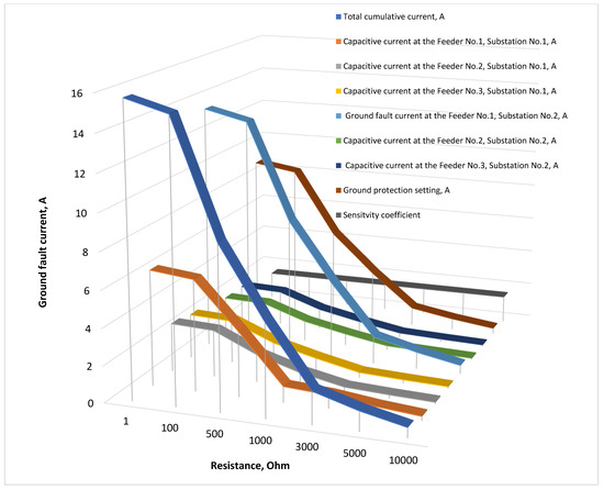
Figure 42.
SPGF with transient resistance at the Feeder No.1, Substation No.2, and capacitive currents in the 10 kV network with the isolated neutral configuration.
At low resistance Rf = 1 Ohm, the SPGF fault current observed by the relay (blue curve) reaches its maximum value of If = 13.49 A. As the transient resistance increases, the ground fault current decreases gradually, falling to If = 0.46 A at Rf = 10,000 Ohm. The capacitive currents behave similarly: they are highest during a metallic fault and decrease non-linearly as the resistance rises. Despite the reduction in fault and capacitive current magnitudes, the sensitivity ratio remains constant at 1.5 across the entire resistance range, ensuring stable relay performance.
Figure 43 presents the ZSV variation during SPGF at Feeder No.1, Substation No.2 for transient resistances from 1 Ohm to 10,000 Ohm.
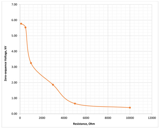
Figure 43.
Zero-sequence voltage during SPGF with transient resistance at the Feeder No.1, Substation No.2 in the 10 kV network with the isolated neutral configuration.
- -
- At the low resistances Rf = 1–100 Ohm, the neutral point is strongly displaced, and the ZSV nearly equals the neutral shift, reaching U0 = 5.77–5.53 kV.
- -
- At the medium resistances Rf = 500–3000 Ohm, the displacement effect weakens, and U0 decreases significantly to 3.25–0.65 kV.
- -
- At the high resistances Rf = 5000–10,000 Ohm, the zero-sequence voltage is minimal, dropping to 0.39–0.20 kV, corresponding to negligible neutral displacement.
This analysis confirms that the ZSV is highly sensitive to the value of transient resistance: high ground conductivity produces strong neutral potential shifts, whereas high-resistance faults generate only weak displacement, making fault detection more challenging.
Figure 44 illustrates the angular difference between the zero-sequence current of the faulty feeder and those of the unfaulted feeders as a function of transient resistance.
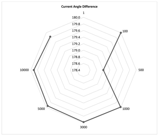
Figure 44.
Current angle difference during SPGF with transient resistance at the Feeder No.1, Substation No.1 in the 10 kV network with the isolated neutral configuration.
- -
- At the low resistances Rf = 1–100 Ohm, the ground fault current is relatively high. The angular difference remains exactly 180°, indicating perfect phase opposition between the faulty feeder’s zero-sequence current and the vector sum of the healthy feeders’ capacitive currents.
- -
- At the medium resistances Rf = 500–3000 Ohm, the ground fault current magnitude decreases as resistance increases. The angular difference reduces slightly to about 179.00°, but still indicates nearly complete opposition, ensuring that the faulted feeder remains easily identifiable.
- -
- At the high resistances Rf = 5000–10,000 Ohm, the ground fault current becomes very weak, approaching the capacitive current magnitudes. The angular difference stabilizes around 179.83°, representing only a minimal 1° deviation.
This result demonstrates the robustness of angle-based discrimination, as the faulted feeder can still be reliably identified even when the ground fault current is extremely low.
Figure 45 shows the variation of the loop integrity coefficient β as transient resistance increases.
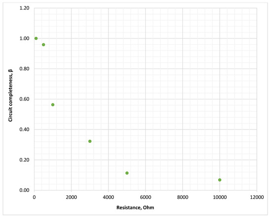
Figure 45.
Loop integrity coefficient during SPGF with transient resistance at the Feeder No.1, Substation No.2 in the 10 kV network with the isolated neutral configuration.
- -
- At the low resistances Rf = 1–100 Ohm, the loop integrity coefficient, β ≈ 1–0.96, the fault current is high, and the neutral point is strongly displaced.
- -
- At the medium resistances Rf = 500–3000 Ohm, the loop integrity coefficient, β decreases progressively from 0.56 to 0.11, indicating a reduction in ground fault severity and weaker neutral potential shift.
- -
- At the high resistances Rf = 5000–10,000 Ohm, the loop integrity coefficient, β reaches very low values of 0.07–0.03, meaning the ground fault current and associated displacement become minimal, making detection more challenging.
Figure 46 shows that the ZS current at the faulty Feeder No.1, Substation No.2 has the largest magnitude and shares the same phase as the unfaulted Feeder No.1, Substation No.1. Both are oriented opposite to the capacitive currents of the remaining healthy feeders, with the phase difference being close to ∠180°.
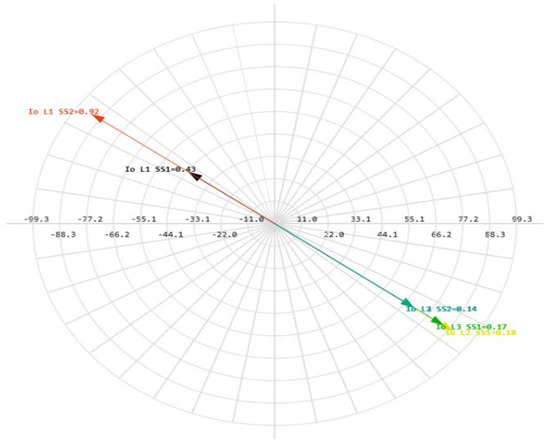
Figure 46.
Phasor diagram for SPGF at the Feeder No.1, substation No.2, and capacitive currents in the 10 kV network with the isolated neutral configuration.
Importantly, the ZS current amplitude at the faulty feeder (Substation No.2) is greater than that at the unfaulted Feeder No.1, Substation No.1. Since the protection at Substation No.1 includes a time delay of 300 ms, the relay at Substation No.2 will operate faster. This ensures selective protection:
- -
- In the case of high-resistance SPGF, the relay at Substation No.2 issues an alarm signal.
- -
- In the case of a bolted, low-resistance SPGF, the relay issues a trip signal, opening the circuit breaker (CB).
Thus, coordinated relay operation ensures reliable fault detection and discrimination, even for high-resistance SPGFs.
Figure 46 illustrates the phasor relations during SPGF at Feeder No.1, Substation No.2. In the case of a bolted SPGF (low transient resistance), the fault current reaches several tens of amperes, whereas under high-resistance SPGF, the current magnitude drops to tenths of an ampere. Despite the reduction, the phasor relationships remain consistent: the SPGF current vector at the faulty feeder is directly opposed to the combined capacitive currents of the unfaulted feeders, ensuring reliable fault detection even at high resistance values.
6.4. Analysis of SPGF Current with Different Transient Resistances on the Substation No.2 Bus in the 10 kV Network with the Isolated Neutral Configuration
Table 25 provides calculated cumulative currents and individual feeder capacitive currents for transient resistance values ranging from 1 Ohm to 10,000 Ohm.
Table 25.
SPGF current values with different transient resistances on the Substation No.2 bus and capacitive currents in the 10 kV network with the isolated neutral configuration.
- -
- At Rf = 1 Ohm, the cumulative current reaches 15.75 A∠50.24°, with the faulty feeder current magnitude in the tens of amperes.
- -
- As resistance increases to Rf = 500–3000 Ohm, the fault current magnitude decreases substantially (from 8.87 A to 1.78 A), while the corresponding phasor angles progressively shift.
- -
- At high resistances (Rf = 5000–10,000 Ohm), the cumulative current reduces further (1.07–0.54 A), approaching the same order as the individual capacitive currents (0.07–0.15 A).
This non-linear reduction emphasizes the strong influence of transient resistance on the fault current, with significant consequences for relay sensitivity.
Table 26 summarizes how system parameters vary with transient resistance.
Table 26.
Dependence of circuit completeness, sensitivity ratio, zero-sequence voltage, and current angle difference from transient resistance during single phase ground fault on the Substation No.2 bus.
- -
- At the low resistances Rf = 1–100 Ohm, the loop integrity coefficient β is close to 1.00–0.96, the zero-sequence voltage reaches its maximum 5.77–5.53 kV, and the current angle difference is 0°, reflecting strong neutral displacement and clear fault signature.
- -
- At the medium resistances Rf = 500–3000 Ohm, the loop integrity coefficient β decreases progressively to 0.56–0.11, and the ZSV drops from 3.25 kV to 0.65 kV, showing weakened neutral potential shift while maintaining stable phase relations.
At the high resistances Rf = 5000–10,000 Ohm, the loop integrity coefficient β falls below 0.07, with the zero-sequence voltage as low as 0.20 kV. The angle difference remains essentially constant 0.00–0.01°, signifying that phasor-based discrimination remains robust even under high-resistance SPGF conditions.
Figure 47 presents the variation of the SPGF current and capacitive currents at different transient resistances ranging from Rf = 1 Ohm to Rf = 10,000 Ohm on the Substation No.2 bus. The dependency is non-linear, with the SPGF current gradually decreasing as the transient resistance increases. The cumulative current at the fault location (yellow curve) reaches a maximum of If = 15.75 A at Rf = 1 Ohm, while at high resistance values Rf = 10,000 Ohm, it drops to If = 0.54 A.
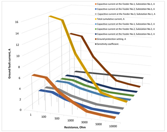
Figure 47.
Ground fault current with the transient resistance on the Substation No.2 bus and capacitive currents in the 10 kV network with the isolated neutral configuration.
The zero-sequence currents contributed by the unfaulted feeders initially equal their respective capacitive currents at the low transient resistance Rf = 1 Ohm. As the transient resistance increases, these currents decrease proportionally, maintaining the same phase angle relationship. Importantly, the sensitivity ratio remains constant at 1.5 across the entire resistance range from Rf = 1 Ohm to Rf = 10,000 Ohm.
Figure 48 illustrates the dependence of ZSV on the transient resistance during SPGF at the Substation No.2 bus. At the low resistance faults Rf = 1–100 Ohm), the neutral voltage displacement is significant, and the ZSV coincides with the neutral shift, reaching values in the range: U0 = 5.77–5.53 kV.
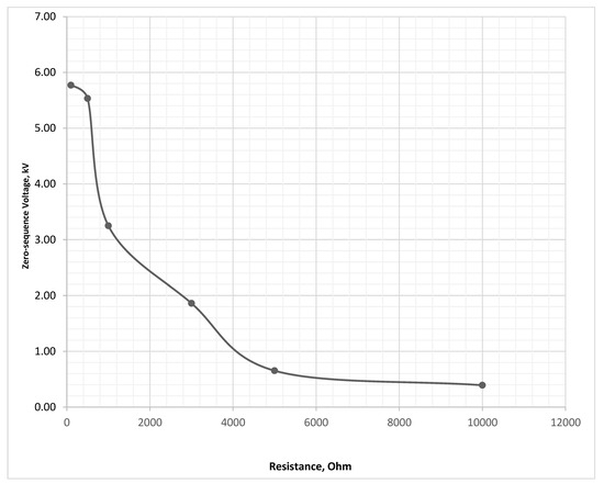
Figure 48.
Zero-sequence voltage during SPGF with transient resistance on the Substation No.2 bus in the 10 kV network with the isolated neutral configuration.
For the medium resistance faults Rf = 500–3000 Ohm, the ZSV decreases substantially, ranging between U0 = 3.25 and 0.65 kV.
At the high resistance faults Rf = 5000–10,000 Ohm, the ZSV is minimal, falling within U0 = 0.39–0.20 kV, which corresponds to the lowest level of neutral point displacement in the system.
Figure 49 illustrates the current angle difference at various transient resistance values. At the low resistance faults Rf = 1–100 Ohm, the SPGF current magnitude is high, and the angle difference remains nearly 0°. This indicates that the unfaulted feeder currents are aligned in the same direction, confirming that the SPGF location is on the busbars.
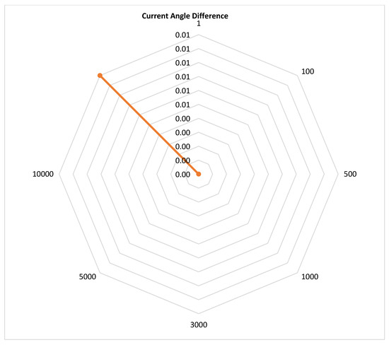
Figure 49.
Current angle difference during SPGF with transient resistance on the Substation No.2 bus in the 10 kV network with the isolated neutral configuration.
At the medium resistance values Rf = 500–3000 Ohm, the SPGF current decreases with increasing resistance, while the angle difference remains close to 0.01°. This demonstrates that the currents still maintain nearly identical phase angles, and the directional signature of the faulted feeder remains distinguishable.
At the high resistance values Rf = 5000–10,000 Ohm, the ground fault current reaches its lowest level, and the angle difference increases slightly to 0.15°. Even under these conditions, the phase relationship is sufficiently reliable to ensure correct fault identification. This behavior confirms that directional detection remains effective, even when the ground fault current magnitude is very small.
Figure 50 shows the change in the loop integrity coefficient as the transient resistance varies. For the low resistance faults Rf = 1–100 Ohm, the loop integrity coefficient remains in the range of β = 1.0–0.96, corresponding to high SPGF currents and a significant neutral point displacement.
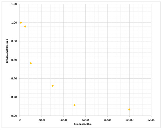
Figure 50.
Loop integrity coefficient during SPGF with transient resistance on the Substation No.2 bus in the 10 kV network with the isolated neutral configuration.
At the medium resistances Rf = 500–3000 Ohm, the loop integrity coefficient decreases gradually to values of 0.56–0.11, indicating a reduction in fault current and a weakened ability to shift the neutral potential.
For the high resistance values Rf = 5000–10,000 Ohm, the loop integrity coefficient decreases further to β = 0.07–0.03, where the SPGF current, capacitive currents, and zero-sequence voltage are all at their lowest magnitudes.
As shown in Figure 51, the capacitive currents of the unfaulted feeders are equal to their respective capacitances, with directions aligned and angle shifts nearly equal to ∠0°. However, the phasor diagram reveals that the zero-sequence current at Feeder No.1 of Substation No.1 has an opposite angle compared to the capacitive currents of the other unfaulted feeders.
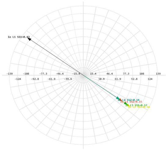
Figure 51.
Phasor diagram for SPGF on the Substation No.2 bus and capacitive currents in the 10 kV network with the isolated neutral configuration. The minimum current in the secondary circuit that the ground overcurrent protection can detect depends on the relay sensitivity and the system configuration. Modern microprocessor relays can usually detect secondary currents of 0.01 to 0.05 A. For example, let us choose a transient resistance at the point of ground fault protection, Rf = 5000 Ohm. Let us calculate the ground overcurrent settings.
This occurs because the ground fault current flows through Feeder No.1 of Substation No.1 toward the fault location at the Substation No.2 bus. Since Feeder No.1 at Substation No.1 is equipped with a 300 ms time delay, the protection at Substation No.2 operates faster. Consequently, in the event of a high-resistance SPGF, the relay at Substation No.2 issues an alarm signal at the bus, whereas in the case of a bolted SPGF, it trips the incomer CB to clear the fault.
In the case of a bolted SPGF on the Substation No.2 bus, the ground fault current magnitude is approximately tens of amperes. For SPGF with the highest transient resistance, the current magnitude reduces to tenths of an ampere.
In the following subsection, the SPGF current will be calculated for fault conditions on Feeder No.1 at Substation No.1 bus and on Feeder No.1 at Substation No.2 bus. Based on these results, the ground overcurrent protection settings will be determined, and the corresponding relay operation and disturbance records will be analyzed.
In case of the bolted SPGF on the Substation No.2 bus, the SPGF current is about ten amperes, and in case of SPGF with the highest transient resistance, the SPGF current reaches tenths of an ampere.
Let us calculate the SPGF considering the transient resistance at the Feeder No.1, Substation No.1 bus and at the Feeder No.1, Substation No.2 bus and calculate the ground overcurrent settings, analyze the protection operation and examine the disturbance records.
7. Single Phase Ground Fault Calculations with the Transient Resistance of Rf = 5000 Ohm, Calculation of Protection Settings and Modeling at the Feeders No.1 and Bus, Substation No.1 and Feeder No.1 and Bus, Substation No.2
7.1. SPGF Calculations with the Transient Resistance of Rf = 5000 Ohm and Calculation of Settings for SPGFs at the Feeder No.1, Substation No.1 in the 10 kV Network with the Isolated Neutral Configuration
The total SPGF current with the transient resistance of Rf = 5000 Ohm is determined by the following expression:
SPGF at the Feeder No.1, Substation No.1 with the transient resistance Rf = 5000 Ohm will be equal to
In the unfaulted Feeder No.2, Substation No.1, the capacitive current is equal to
The capacitive current in the unfaulted Feeder No.3, Substation No.1 will be equal to
In the unfaulted Feeder No.1, Substation No.2, the capacitive current is equal to
In the unfaulted Feeder No.2, Substation No.2, the capacitive current is equal to
The capacitive current in the unfaulted Feeder No.3, Substation No.2 will be equal to
7.2. SPGF Calculation with the Transient Resistance of Rf = 5000 Ohm and Calculation of Settings for SPGF on the Substation No.1 Bus in the 10 kV Network with the Isolated Neutral Configuration
The total SPGF current with the transient resistance of Rf = 5000 Ohm is determined by the following expression:
The capacitive current in the unfaulted Feeder No.1, Substation No.1 is equal to
The capacitive current in the unfaulted Feeder No.2, Substation No.1 will be equal to
The capacitive current in the unfaulted Feeder No.3, Substation No.1 is equal to
In the unfaulted Feeder No.1, Substation No.2, the capacitive current is equal to
In the unfaulted Feeder No.2, Substation No.2, the capacitive current is equal to
The capacitive current in the unfaulted Feeder No.3, Substation No.2 will be equal to
We select the CGFPU setting for SPGF for Substation No.1
When selecting the CGFPU setting for SPGF with the transient resistance of Rf = 5000 Ohm, we select the smallest one from the calculation, Iop = 0.28 A with the sensitivity ratio of Ks = 1.5 and with issuing an alarm signal. The angle between SPGF at one of the feeders and capacitive currents, we select ± 200 from 1800.
7.3. Modeling of SPGF with the Transient Resistance of Rf = 5000 Ohm at the Feeder No.1, Substation No.1 in the 10 kV Network with the Isolated Neutral Configuration
Figure 52 shows the single line diagram with SPGF with the transient resistance Rf = 5000 Ohm at the Feeder No.1, Substation No.1 in the 10 kV network with the isolated neutral configuration. At the Incomer, Substation No.1, the zero-sequence current is IZSCT = 0.02 A, and the zero-sequence current angle is φ = −34.79°. At the Feeder No.1, Substation No.1, the zero-sequence current is IZSCT = 0.44 A, and the zero-sequence current angle is φ = 145.17°. At the Feeder No.2, Substation No.1, the zero-sequence current is IZSCT = 0.19 A, and the zero-sequence current angle is φ = −34.81°. At the Feeder No.3, Substation No.1, the zero-sequence current is IZSCT = 0.17 A, and the zero-sequence current angle is φ = −34.81°. At the Incomer, Substation No.2, the zero-sequence current is IZSCT = 0.49 A, and the zero-sequence current angle is φ = 145.26°. At the Feeder No.1, Substation No.2, the zero-sequence current is IZSCT = 0.15 A, and the zero-sequence current angle is φ = −34.75°. At the Feeder No.2, Substation No.2, the zero-sequence current is IZSCT = 0.14 A, and the zero-sequence current angle is φ = −34.74°. At the Feeder No.3, Substation No.2, the zero-sequence current is IZSCT = 0.14 A, and the zero-sequence current angle is φ = −34.74°.
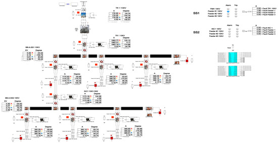
Figure 52.
Single-line diagram with SPGF with the transient resistance of Rf = 5000 Ohm at the Feeder No.1, Substation No.1 in the 10 kV network with the isolated neutral configuration.
Figure 53 presents the disturbance recording of SPGF with transient resistance of Rf = 5000 Ohm at the Feeder No.1, Substation No.1 in the 10 kV network with the isolated neutral configuration. The total cumulative SPGF current on the phase A with the transient resistance Rf = 5000 Ohm is 1.09 A and the angle of the zero-sequence current is φ = 146.17°. The SPGF on the phase A with the transient resistance Rf = 5000 Ohm, has a greater magnitude and a shift of about 180–185° from the phasor of the capacitive currents of the unfaulted Feeders No.2 and 3 in the Substation No.1 and Feeders No.1, 2, and 3 in the Substation No.2. Due to the fact that the SPGF current exceeds the ground overcurrent setting, an alarm signal at the Feeder No.1, Substation No.1 is issued (Figure 52).
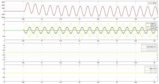
Figure 53.
Disturbance record of SPGF with transient resistance of Rf = 5000 Ohm at the Feeder No.1, Substation No.1 in the 10 kV network with the isolated neutral configuration.
7.4. Modeling of SPGF with the Transient Resistance of Rf = 5000 Ohm on the Substation No.1 Bus in the 10 kV Network with the Isolated Neutral Configuration
Figure 54 shows the single line diagram with SPGF with the transient resistance of Rf = 5000 Ohm on the Substation No.1 bus in the 10 kV network with the isolated neutral configuration. At the Incomer, Substation No.1, the zero-sequence current is IZSCT = 0.02 A, and the zero-sequence current angle is φ = −33.43°. At the Feeder No.1, Substation No.1, the zero-sequence current is IZSCT = 0.65 A, and the zero-sequence current angle is φ = −33.35°. At the Feeder No.2, Substation No.1, the zero-sequence current is IZSCT = 0.19 A, and the zero-sequence current angle is φ = −33.42°. At the Feeder No.3, Substation No.1, the zero-sequence current is IZSCT = 0.17 A, and the zero-sequence current angle is φ = −33.41°. At the Incomer, Substation No.2, the zero-sequence current is IZSCT = 0.49 A, and the zero-sequence current angle is φ = 146.67°. At the Feeder No.1, Substation No.2, the zero-sequence current is IZSCT = 0.16 A, and the zero-sequence current angle is φ = −33.35°. At the Feeder No.2, Substation No.2, the zero-sequence current is IZSCT = 0.14 A, and the zero-sequence current angle is φ = −33.34°. At the Feeder No.3, Substation No.2, the zero-sequence current is IZSCT = 0.14 A, and the zero-sequence current angle is φ = −33.34°. Figure 23 also illustrates the correct detection and localization of a single-phase ground fault with a transient resistance of Rf = 5000 Ohm located on the substation No.1 bus. The CGFPU protection system correctly identifies the fault at the incomer by analyzing the magnitude and angle of the zero-sequence current and issues a selective alarm without false operation on unfaulted feeders, confirming high reliability and sensitivity even under high-resistance fault conditions.

Figure 54.
Single line diagram with SPGF with the transient resistance of Rf = 5000 Ohm on the Substation No.1 bus in the 10 kV network with the isolated neutral configuration.
Figure 55 presents the disturbance record of SPGF with the transient resistance of Rf = 5000 Ohm on the Substation No.1 bus in the 10 kV network with the isolated neutral configuration. The total cumulative SPGF current on the phase A with the transient resistance of Rf = 5000 Ohm is 1.09 A and the angle of the zero-sequence current is φ = −33.43°. The SPGF on the phase A with the transient resistance of Rf = 5000 Ohm, has a greater magnitude, has the same direction, and a shift of about 0–5° from the phasor of the capacitive currents of the unfaulted Feeders No.1, 2, and 3 in the Substation No.1 and Feeders No.1, 2, and 3 in the Substation No.2. Due to the fact that the SPGF current exceeds the ground overcurrent setting, an alarm signal on the Substation No.1 bus is issued (Figure 23).
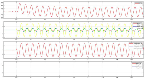
Figure 55.
Disturbance record of SPGF with transient resistance of Rf = 5000 Ohm on the Substation No.1 bus in the 10 kV network with the isolated neutral configuration.
7.5. SPGF Calculation with the Transient Resistance of Rf = 5000 Ohm and Calculation of Settings for SPGF at the Feeder No.1, Substation No.2 in the 10 kV Network with the Isolated Neutral Configuration
The total SPGF with the transient resistance of Rf = 5000 Ohm is determined by the following expression:
In the unfaulted Feeder No.1, Substation No.1, the capacitive current is defined as follows:
The capacitive current in the unfaulted Feeder No.2, Substation No.1 is equal to
In the unfaulted Feeder No.3, Substation No.1, the capacitive current is equal to
The SPGF current at the Feeder No.1, Substation No.2 with the transient resistance of Rf= 5000 Ohm amounts to
In the unfaulted Feeder No.2, Substation No.2, the capacitive current is equal to
The capacitive current in the unfaulted Feeder No.3, Substation No.2 amounts to
7.6. SPGF Calculation with the Transient Resistance of Rf = 5000 Ohm and Calculation of Settings for SPGF on the Substation No.2 Bus in the 10 kV Network with the Isolated Neutral Configuration
The total SPGF current with the transient resistance of Rf = 5000 Ohm is determined by the following expression:
The capacitive current in the unfaulted Feeder No.1, Substation No.1 is equal to
The capacitive current in the unfaulted Feeder No.2, Substation No.1 amounts to
In the unfaulted Feeder No.3, Substation No.1, the capacitive current is defined as follows:
In the unfaulted Feeder No.1, Substation No.2, the capacitive current is calculated as follows:
In the unfaulted Feeder No.2, Substation No.2, the capacitive current is equal to
The capacitive current in the unfaulted Feeder No.3, Substation No.2 will be equal to
We select the CGFPU setting for SPGF for Substation No.2.
When selecting the CGFPU setting for SPGF with the transient resistance of Rf = 5000 Ohm, the smallest calculated operating setting is selected Iop = 0.1 A with the sensitivity ratio of Ks = 1.5. In this case, the CGFPU issues an alarm signal. For the angle between SPGF at one of the feeders and capacitive currents, we select ±20° from 180°. For SPGF on the bus, the angle between the capacitive currents, we select ±20° from 0°.
7.7. Modeling of SPGF with the Transient Resistance of Rf = 5000 Ohm at the Feeder No.1, Substation No.2 in the 10 kV Network with the Isolated Neutral Configuration
Figure 56 shows the single line diagram with SPGF with the transient resistance of Rf = 5000 Ohm at the Feeder No.1, Substation No.2 in the 10 kV network with the isolated neutral configuration. At the Incomer, Substation No.1, the zero-sequence current is IZSCT = 0.02 A, and the zero-sequence current angle is φ = −35.73°. At the Feeder No.1, Substation No.1, the zero-sequence current is IZSCT = 0.43 A, and the zero-sequence current angle is φ = 144.20°. At the Feeder No.2, Substation No.1, the zero-sequence current is IZSCT = 0.19 A, and the zero-sequence current angle is φ = −35.78°. At the Feeder No.3, Substation No.1, the zero-sequence current is IZSCT = 0.17 A, and the zero-sequence current angle is φ = −35.79°. At the Incomer, Substation No.2, the zero-sequence current is IZSCT = 0.59 A, and the zero-sequence current angle is φ = −35.79°. At the Feeder No.1, Substation No.2, the zero-sequence current is IZSCT = 0.92 A, and the zero-sequence current angle is φ = 144.23°. At the Feeder No.2, Substation No.2, the zero-sequence current is IZSCT = 0.14 A, and the zero-sequence current angle is φ = −35.72°. At the Feeder No.3, Substation No.2, the zero-sequence current is IZSCT = 0.14 A, and the zero-sequence current angle is φ = −35.72°.
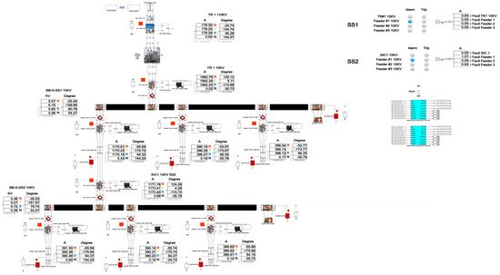
Figure 56.
Single line diagram with SPGF with transient resistance of Rf = 5000 Ohm at the Feeder No.1, Substation No.2 in the 10 kV network with the isolated neutral configuration.
Figure 57 shows the disturbance record of SPGF with the transient resistance of Rf = 5000 Ohm at the Feeder No.1, Substation No.2 in the 10 kV network with the isolated neutral configuration. The total cumulative SPGF current on the phase A with the transient resistance Rf = 5000 Ohm is 1.07 A and the angle of the zero-sequence current is φ = 144.23°. The SPGF on the phase A with the transient resistance Rf = 5000 Ohm, has a greater magnitude and a shift of about 180–185° from the phasor of the capacitive currents of the unfaulted Feeders No.2 and 3 in the Substation No.2 and Feeders No.1, 2, and 3 in the Substation No.1. Due to the fact that the SPGF current exceeds the ground overcurrent setting, an alarm signal at the Feeder No.1, Substation No.2 is issued (Figure 26).
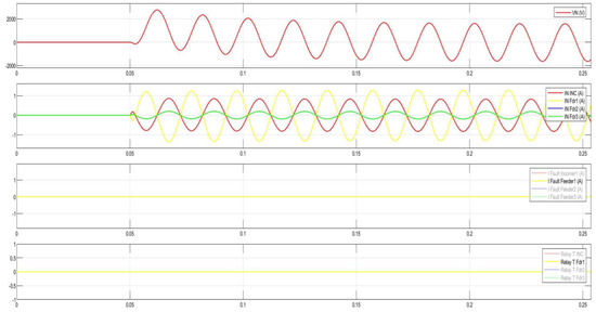
Figure 57.
Disturbance record of SPGF with transient resistance of Rf = 5000 Ohm at the Feeder No.1, Substation No.2 in the 10 kV network with the isolated neutral configuration.
7.8. Modeling of SPGF with the Transient Resistance of Rf = 5000 Ohm on the Substation No.2 Bus in the 10 kV Network with the Isolated Neutral Configuration
Figure 58 shows the single line diagram with SPGF with the transient resistance of Rf = 5000 Ohm on the Substation No.2 bus in the 10 kV network with the isolated neutral configuration. At the Incomer, Substation No.1, the zero-sequence current is IZSCT = 0.02 A, and the zero-sequence current angle is φ = −35.50°. At the Feeder No.1, Substation No.1, the zero- sequence current is IZSCT = 0.43 A, and the zero-sequence current angle is φ = 144.44°. At the Feeder No.2, Substation No.1, the zero-sequence current is IZSCT = 0.19 A, and the zero-sequence current angle is φ = −35.55°. At the Feeder No.3, Substation No.1, the zero-sequence current is IZSCT = 0.17 A, and the zero-sequence current angle is φ = −35.55°. At the Incomer, Substation No.2, the zero-sequence current is IZSCT = 0.59 A, and the zero-sequence current angle is φ = −35.55°. At the Feeder No.1, Substation No.2, zero-sequence current is IZSCT = 0.15 A, and the zero-sequence current angle is φ = −35.49°. At the Feeder No.2, Substation No.2, the zero-sequence current is IZSCT = 0.14 A, and the zero-sequence current angle is φ = −35.48°. At the Feeder No.3, Substation No.2, the zero-sequence current is IZSCT = 0.14 A, and the zero-sequence current angle is φ = −35.48°.
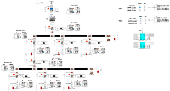
Figure 58.
Single line diagram with SPGF with transient resistance of Rf = 5000 Ohm on the Substation No.2 bus in the 10 kV network with the isolated neutral configuration.
Figure 59 presents the disturbance record of SPGF with the transient resistance of Rf = 5000 Ohm on the Substation No.2 bus in the 10 kV network with the isolated neutral configuration. The total cumulative SPGF current on the phase A with the transient resistance of Rf = 5000 Ohm is 1.07 A and the angle of the zero-sequence current is φ = −33.50°. The SPGF on the phase A with the transient resistance of Rf = 5000 Ohm, has a greater magnitude, has the same direction and a shift of about 0–5° from the phasor of the capacitive currents of the unfaulted Feeders No.1, 2, and 3 in the Substation No.1 and Feeders No.1, 2, and 3 in the Substation No.2. Due to the fact that the SPGF current exceeds the ground overcurrent setting, an alarm signal on the Substation No.2 bus is issued (Figure 41).
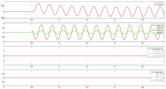
Figure 59.
Disturbance record of SPGF with transient resistance of Rf = 5000 Ohm on the Substation No.2 bus in the 10 kV network with the isolated neutral configuration.
8. Discussion
The modeling and analysis results confirm the effectiveness of the proposed CGFPU for selective detection of SPGFs with the transient resistance in the MV networks with various neutral configurations. In contrast to the conventional methods, which rely exclusively on ZSC magnitude measurements or directional relays, harmonic content or transient based protections, the combined use of ZSC angle and magnitude significantly improves fault identification accuracy under challenging conditions, particularly for high-resistance faults.
A key observation is the non-linear dependence of both SPGF current magnitude and capacitive current magnitude on the transient resistance value. As the fault resistance increases from Rf = 1 Ohm to Rf = 10,000 Ohm, the SPGF current decreases sharply, approaching only tenths of an ampere at high resistance levels. Despite this reduction, the CGFPU algorithm reliably identifies the faulty feeder by detecting the characteristic 180° phase opposition between the faulty feeder’s ZSC and the capacitive ZSC of the unfaulted feeders. This demonstrates that the method maintains robustness across a wide resistance range, even when traditional amplitude-based approaches fail.
Another important finding is related to faults occurring on the busbars. In such cases, the ZSC phasors of all outgoing feeders remain aligned in direction, with only slight angular deviations. This behavior enables the CGFPU to correctly differentiate between feeder faults and bus faults—an essential capability for selective protection in branched distribution networks.
The simulations further show that slight angular deviations at higher transient resistances Rf = 3000–5000 Ohm do not impair fault selectivity, since the algorithm tolerates deviations up to ±20° from the ideal 180° signature. The protection system also demonstrates flexibility in operating modes as follows:
- -
- For high-resistance faults Rf = 10,000 Ohm, the CGFPU correctly issues an alarm signal, avoiding unnecessary feeder disconnection and preserving network continuity.
- -
- For low-resistance (bolted) faults Rf = 1 Ohm, the CGFPU promptly generates a trip signal, ensuring fast isolation of the faulty element and enhancing operational safety.
- -
- Even under admittance imbalance ΔY = 15%, the fault current error stays <0.5%, proving that admittance-induced distortion affects only neutral voltage, not the operating current. Based on the findings, with ±20° phase-angle deviation, the CGFPU remains selective and reliable.
- -
- The computed loop integrity coefficient β decreases exponentially with Rf. For low-resistance faults, the loop integrity coefficient β ≈ 1 indicates a complete current loop; as Rf exceeds 3 kOhm, the loop integrity coefficient β drops below 0.1, signifying that the circuit becomes nearly open.
Nevertheless, the CGFPU successfully detects such weak faults because its operation depends on the directional opposition of the feeder ZSC phasors (≈180°) rather than on the current magnitude itself. This characteristic ensures reliable detection even when the measurable current nearly vanishes.
- -
- The sensitivity ratio Ks remains practically constant at about 1.5 across all simulated capacitances and fault impedances. This constancy confirms that the CGFPU satisfies the minimum sensitivity requirement Ks ≥ 1.3–1.5 stipulated by PUE RK, thereby ensuring stable performance independent of Rf and network grounding mode.
- -
- The analysis of ground-overcurrent pickup currents shows that the required settings decrease sharply with increasing Rf and level off beyond 4–5 kOhm.
Larger network capacitance necessitates proportionally higher initial pickup levels to accommodate increased capacitive charging current.
For small-capacitance systems C0Σ ≤ 2 µF, pickup currents remain below 7 A even at low Rf, whereas for high-capacitance systems C0Σ ≥ 10 µF they reach ≈36 A at Rf = 1 Ohm.
The CGFPU has shown strong immunity to unbalanced charging currents and natural line capacitances under unfaulted conditions, effectively preventing nuisance trips. Its centralized architecture further improves coordination between substations and eliminates overlapping protection zones, a common drawback of decentralized schemes.
Compared to the existing protection methods, the proposed method offers the following:
- -
- simpler implementation,
- -
- faster detection times,
- -
- reduced computational burden,
- -
- and high accuracy even in networks with fluctuating capacitances and fault resistances.
Finally, the flexibility of the proposed method makes it well-suited for integration into future smart grids and microgrids, where the presence of distributed energy resources and dynamic load patterns will further complicate SPGF detection. By incorporating advanced features such as adaptive thresholding and transient feature analysis, the CGFPU concept can be expanded into a new generation of intelligent, high-resolution protection systems for the MV networks.
In summary, the developed method and device structure not only address the urgent challenge of detecting SPGFs with transient resistance but also establish a foundation for next-generation selective protection strategies in evolving power systems.
9. Conclusions
In this study, the values of SPGF parameters were determined for different transition resistances, transient processes during SPGF were modeled, and the operation of the CGFPU was evaluated. A protection scheme and algorithm for detecting and protecting isolated neutral networks from SPGF with transition resistance were developed. Based on the results of analytical calculations and MATLAB Simulink modeling, the following conclusions can be drawn:
- -
- The dependencies of the ZSC of feeders in isolated neutral networks on the value of transition resistance and the zero-sequence circuit parameters were established. These dependencies make it possible to evaluate the loop integrity coefficient during ground faults. Analytical expressions for SPGF considering transition resistance, loop integrity coefficient, pickup levels, offset factors, and protection sensitivity ratios were obtained. The corresponding setting values for ground overcurrent protection, enabling operation in alarm or trip mode, were defined.
- -
- An algorithm for selective identification of the faulted zone in both internal (feeder) and external (bus) SPGF with transition resistance was proposed.
- -
- Functional diagrams of the developed relay protection device against SPGF were prepared, and the operation principles of its functional blocks and modules were described.
- -
- The proposed device ensures selective operation during feeder maintenance or disconnection and is capable of detecting both single-phase and multiple ground faults.
- -
- Transient process modeling confirmed the correct functioning of the centralized relay protection algorithm against SPGF in MATLAB Simulink. Simulation results showed the following:
- The SPGF current phasor in the faulty feeder is shifted by 180° relative to the capacitive current phasors, while the capacitive currents of unfaulted feeders align in phase.
- Nonlinear variations of SPGF currents and capacitive currents occur with the increase of transition resistance Rf from 1 Ohm to 10,000 Ohm.
- The angular difference between the SPGF current of the faulty feeder and the capacitive currents of the healthy feeders slightly increases with the growth of Rf.
- For SPGF occurring on busbars, capacitive current magnitudes change proportionally with Rf and match the self-capacitance values under bolted ground fault conditions, with only minor changes in phase angles.
- -
- The proposed relay protection device is simple in construction and operation. Unlike existing methods, it requires only a ZSC signal and does not rely on auxiliary signals such as zero-sequence voltage, higher harmonic content, multifrequency signals, or additional complex hardware including voltage transformers.
- -
- The CGFPU demonstrates selective and reliable operation: it generates an alarm signal at Rf = 10,000 Ohm and trips at Rf = 1 Ohm, depending on the trip settings. It is resistant to unbalanced charging currents and inrush currents.
- -
- The CGFPU has a universal application and can be used in isolated, compensated, and resistively grounded networks.
Due to its independence from voltage magnitude, insensitivity to power flow direction, and robustness against inverter-based distortions, the device is well-suited for smart grids, microgrids, and renewable energy networks where inverter switching and weak grid conditions introduce harmonics and fluctuations.
Author Contributions
Conceptualization, K.T.; methodology, M.J.; software, M.J.; validation, A.Z.; formal analysis, S.S. and K.T.; investigation, T.S.; resources, A.B. and G.S.; data curation, T.S.; writing—original draft preparation, A.Z., G.S., S.S. and K.T.; writing—review and editing, A.B., T.S. and M.J.; visualization, A.Z. and M.J.; supervision, K.T.; project administration, A.Z., M.J. and K.T.; funding acquisition, S.S., G.S., A.B. and T.S. All authors have read and agreed to the published version of the manuscript.
Funding
This research received no external funding.
Data Availability Statement
The original contributions presented in this study are included in the article. Further inquiries can be directed to the corresponding author.
Acknowledgments
This work was performed at the Institute of Energy and Green Technologies, Almaty University of Power Engineering and Telecommunications, named after G. Daukeyev which is gratefully acknowledged by the authors.
Conflicts of Interest
The authors declare no conflicts of interest.
Glossary
| ASR | Arc Suppression Reactor |
| CGFPU | Centralized Ground Fault Protection Unit |
| CI-PPFL | Class-imbalance privacy-preserving federated learning |
| CL | Cable Line |
| CT | Current Transformer |
| DS | Distribution Substation |
| kA | Kiloampere |
| kV | Kilovolt |
| MV | Medium Voltage |
| OHL | Overhead Line |
| OV | Overvoltage |
| PUE RK | Rules for Electrical Installations of the Republic of Kazakhstan |
| RP | Relay Protection |
| SGLQRDNN | Non-crossing sparse-group Lasso-quantile regression deep neural network |
| SPGF | Single Phase Ground Fault |
| SS | Substation |
| VT | VT Voltage Transformer |
| XLPE | Cross-linked Polyethylene |
| ZSC | ZSC Zero Sequence Current |
| ZSCT | ZSC Zero Sequence Current Transformer |
| ZSV | Zero Sequence Voltage |
References
- Zhang, X.; Xu, B.; Pan, Z.; Wei, P. Study on single-phase earthed faulty feeder selection methods in non-solidly grounded systems. In Proceedings of the Third International Conference on Electric Utility Deregulation and Re-structuring and Power Technologies (DRPT 2008), Nanjing, China, 6–9 April 2008; pp. 1836–1840. [Google Scholar]
- Ma, J.; Yan, X.; Fan, B.; Liu, C.; Thorp, J.S. A novel line protection scheme for a single phase-to-ground fault based voltage phase comparison. IEEE Trans. Power Deliv. 2016, 31, 2018–2027. [Google Scholar] [CrossRef]
- Abbas, A.K.; Hamad, S.; Hamad, N. Singleline to ground fault detection and location in medium voltage distribu-tion system based on neural network. Indones. J. Electr. Eng. Comput. Sci. 2021, 23, 621–632. [Google Scholar] [CrossRef]
- Mukherjee, A.; Kundu, P.K.; Das, A. A supervised principal component analysis-based approach of fault localiza-tion in transmission lines for single line to ground faults. Electr. Eng. 2021, 103, 2113–2126. [Google Scholar] [CrossRef]
- Mardegan, C.; Rifaat, R.S. Insights into Applications of IEEE Standards for Ground-Fault Protection in Industrial and Commecial Power Systems. IEEE Trans. Ind. Appl. 2015, 51, 2854–2861. [Google Scholar] [CrossRef]
- Gazprom. Guidelines for Selecting the Grounding Mode of Neutrals in 6 and 10 kV Networks of Subsidiaries and Organizations of OAO “Gazprom”; STO Gazprom 2-1.11-070-2006; Gazprom: Moscow, Russia, 2006; 24p. (In Russian) [Google Scholar]
- Ustinov, D.; Nazarychev, A.; Pelenev, D.; Babyr, K. Investigation of the Effect of Current Protections in Conditions of Single-Phase Ground Fault through Transient Resistance in the Electrical Networks of Mining Enterprises. Energies 2023, 16, 3690. [Google Scholar] [CrossRef]
- Kraszewski, W.; Syrek, P.; Mitoraj, M. Methods of Ferroresonance Mitigation in Voltage Transformers in a 30 kV Power Supply Network. Energies 2022, 15, 9516. [Google Scholar] [CrossRef]
- Rzayeva, S.V.; Mammadov, N.S.; Ganiyeva, N.A. Overvoltages During Single-Phase Earth Fault in Neutral-Isolated Networks (10÷35) kV. J. Energy Res. Rev. 2023, 13, 7–13. [Google Scholar] [CrossRef]
- Shuin, V.A. The influence of the discharge of the faulty phase capacitance on the transient process at ground faults in 3–10 kV cable networks. Electricity 1983, 12, 4–9. (In Russian) [Google Scholar]
- Shuin, V.A. Protection Against Ground Faults in 6–10 kV Electrical Networks; Shuin, V.A., Gusenkov, A.V., Eds.; NTF “Energoprogress”, “Energetik”: Moscow, Russia, 2001; 104p. (In Russian) [Google Scholar]
- Lin, X.; Ke, S.; Gao, Y.; Wang, B.; Liu, P. A selective single phase-to-ground fault protection for neutral ineffec-tively grounded systems. Int. J. Electr. Power Energy Syst. 2011, 33, 1012–1017. [Google Scholar] [CrossRef]
- Henriksen, T. Faulty feeder identification in high impedance grounded network using charge-voltage relationship. Electr. Power Syst. Res. 2011, 81, 1832–1839. [Google Scholar] [CrossRef]
- Huang, S.J.; Wan, H.H. A Method to enhance ground-fault computation. IEEE Power Eng. Lett. IEEE Trans. Power Syst. 2010, 25, 1190–1191. [Google Scholar] [CrossRef]
- Lin, W.M.; Ou, T.C. Unbalanced distribution network fault analysis with hybrid compensation. IET Gen. Transmiss. Distrib. 2011, 5, 92–100. [Google Scholar] [CrossRef]
- Ou, T.C. A novel unsymmetrical faults analysis for microgrid distribution systems. Int. J. Electr. Power Energy Syst. 2012, 43, 1017–1024. [Google Scholar] [CrossRef]
- Andreev, A.A. Analysis of Existing Types of Protection Against Single-Phase Ground Faults and the Conditions for Their Application. Bull. Samara State Tech. Univ. Ser. Tech. Sci. 2021, 4, 56–70. (In Russian) [Google Scholar] [CrossRef]
- Shabad, M.A. (Ed.) Protection Against Single-Phase Ground Faults in 6–35 kV Networks: A Tutorial; Energoprogress: Energetik: Moscow, Russia, 2007; 63p. (In Russian) [Google Scholar]
- Shabad, M.A. (Ed.) Protection Against Single-Phase Ground Faults in 6–35 kV Networks: Lecture Notes; PEIPK: St. Petersburg, Russia, 2002; 51p. (In Russian) [Google Scholar]
- Andreev, V.A. Relay Protection and Automation of Power Supply Systems; Higher School: Moscow, Russia, 2006; 639p. (In Russian) [Google Scholar]
- Fedoseyev, A.M. Relay Protection of Electrical Systems; Energy: Moscow, Russia, 1976; 560p. (In Russian) [Google Scholar]
- Vinokurova, T.Y.; Vorobyova, E.A.; Shuin, V.A. About the choice of the operating frequency range of the device earth fault protection devices based on transient processes in 6–10 kV cable networks. In Proceedings of the IX International Youth Scientific Conf. “Tinchurin Readings”, 4 Volumes. Vol. 1; Abdullazyanov, E.Y., Ed.; Kazan State Power Engineering University: Kazan, Russia, 2014; p. 373. (In Russian) [Google Scholar]
- Hanninen, S. Single phase earth faults in high impedance grounded networks. In Characteristics, Indication and Location [Electronic Resource]; VTT Publications: Espoo, Finland, 2001; 143p, ISBN 951-38-5960-6. [Google Scholar]
- Gelfand, Y.S. Relay Protection of Distribution Networks; Energoatomizdat: Moscow, Russia, 1987; 368p. [Google Scholar]
- Evdokunin, G.A. Selection of the Method of Neutral Grounding in 6–10 kV Networks; Evdokunin, G.A., Gudilin, S.V., Korepanov, A.A., Eds.; Electricity: Moscow, Russia, 1998; Volume No 12, pp. 8–23. (In Russian) [Google Scholar]
- Titenkov, S.S.; Pugachev, A.A. Neutral grounding modes in 6–35 kV networks and organization of relay protection against single-phase ground faults. Energy Expert 2010, 2, 18–25. (In Russian) [Google Scholar]
- Weinstein, P.A. Neutral Grounding Modes in Electrical Systems: A Tutorial; Weinstein, P.A., Kolomiets, N.V., Shestakova, V.V., Eds.; TPU Publishing House: Tomsk, Russia, 2006; 119p. (In Russian) [Google Scholar]
- Yemelyanov, I.N.; Shirkovets, A.I. Current issues of application of resistive and combined neutral grounding in 6–35 kV electrical networks. Energoexpert 2010, 2, 44–50. (In Russian) [Google Scholar]
- Khalilova, F.A.; Boynazarov, B.B. Characteristics of arc-suppressing reactors used to compensate for capacitive fault currents. Probl. Sci. Mosc. 2019, 10, 11–15. (In Russian) [Google Scholar]
- Shirkovets, A.; Sarin, L.; Ilyinykh, M.; Poyachev, V.; Shalin, A. Resistive grounding of neutral in 6–35 kV networks with XLPE cables. Electr. Eng. News 2008, 2, 4. (In Russian) [Google Scholar]
- Ilyinykh, M.; Sarin, L.; Shirkovets, A. Compensated combined grounded neutral. Electr. Eng. News 2016, 5, 16–26. (In Russian) [Google Scholar]
- Lu, S.; Xu, Q.; Jiang, C.; Liu, Y.; Kusiak, A. Probabilistic load forecasting with a non-crossing sparse-group Lasso-quantile regression deep neural network. Energy 2022, 242, 122955. [Google Scholar] [CrossRef]
- Lu, S.; Gao, Z.; Xu, Q.; Jiang, C.; Zhang, A.; Wang, X. Class-imbalance privacy-preserving federated learning for decentralized fault diagnosis with biometric authentication. IEEE Trans. Ind. Inform. 2022, 18, 9101–9111. [Google Scholar] [CrossRef]
- Zhang, J.; Li, C.; Qi, J.; He, J. A Survey on Class Imbalance in Federated Learning. arXiv 2023, arXiv:2303.11673. [Google Scholar] [CrossRef]
- Wen, H.; Liu, X.; Lei, B.; Yang, M.; Cheng, X.; Chen, Z. A privacy-preserving heterogeneous federated learning framework with differential privacy for electricity theft detection in smart grids. Appl. Energy 2025, 378, 124789. [Google Scholar] [CrossRef]
- Arévalo, P.; Benavides, D.; Ochoa-Correa, D.; Ríos, A.; Torres, D.; Villanueva-Machado, C.W. Smart Microgrid Management and Optimization: A Systematic Review. Algorithms 2025, 18, 429. [Google Scholar] [CrossRef]
- Vimal Raj, D. A comprehensive review of microgrid challenges in architectures. J. Electr. Syst. Inf. Technol. 2024, 11, 60. [Google Scholar] [CrossRef]
- IEC 60255-1:2009; Measuring Relays and Protection Equipment—Part 1. Common Requirements Standard International Electrotechnical Commission: Geneva, Switzerland, 2009.
- IEC 61850-8-1; Communication Networks and Systems for Power Utility Automation. International Electrotechnical Commission: Geneva, Switzerland, 2020.


Disclaimer/Publisher’s Note: The statements, opinions and data contained in all publications are solely those of the individual author(s) and contributor(s) and not of MDPI and/or the editor(s). MDPI and/or the editor(s) disclaim responsibility for any injury to people or property resulting from any ideas, methods, instructions or products referred to in the content. |
© 2025 by the authors. Licensee MDPI, Basel, Switzerland. This article is an open access article distributed under the terms and conditions of the Creative Commons Attribution (CC BY) license (https://creativecommons.org/licenses/by/4.0/).