Abstract
High-renewables grids are planned in min but judged in milliseconds; credible studies must therefore resolve both horizons within a single model. Current adequacy tools bypass fast frequency dynamics, while detailed simulators lack multi-hour optimization, leaving investors without a unified basis for sizing storage, shifting demand, or upgrading transfers. We present a two-layer Hierarchical Model Predictive Control framework that links 15-min scheduling with 1-s corrective action and apply it to Germany’s four TSO zones under a stringent zero-exchange stress test derived from the NEP 2045 baseline. Batteries, vehicle-to-grid, pumped hydro and power-to-gas technologies are captured through aggregators; a decentralized optimizer pre-positions them, while a fast layer refines setpoints as forecasts drift; all are subject to inter-zonal transfer limits. Year-long simulations hold frequency within ±2 mHz for 99.9% of hours and below ±10 mHz during the worst multi-day renewable lull. Batteries absorb sub-second transients, electrolyzers smooth surpluses, and hydrogen turbines bridge week-long deficits—none of which violate transfer constraints. Because the algebraic core is modular, analysts can insert new asset classes or policy rules with minimal code change, enabling policy-relevant scenario studies from storage mandates to capacity-upgrade plans. The work elevates predictive control from plant-scale demonstrations to system-level planning practice. It unifies adequacy sizing and dynamic-performance evaluation in a single optimization loop, delivering an open, scalable blueprint for high-renewables assessments. The framework is readily portable to other interconnected grids, supporting analyses of storage obligations, hydrogen roll-outs and islanding strategies.
1. Introduction
The volatility of renewable energy in modern grids requires sophisticated frequency control [1,2,3]. Since 2010, wind and solar have driven the largest expansion of renewables and become integral to modern power grids, supplying around 15% of the global electricity mix in 2024—meanwhile, slowing non-renewable growth and fossil-plant retirements have made renewables the fastest-growing capacity source [4]. As global solar and wind capacities grow, surpassing traditional sources in many regions, the grid’s vulnerability to supply fluctuations increases, stressing the need for advanced management systems to maintain stability [5,6,7]. A key challenge in maintaining a stable power grid is keeping frequency at nominal levels. Achieving this requires balancing power generation with demand, necessitating precise coordination to adjust to evolving grid conditions [8]. Traditional control algorithms are inadequate for future electrical energy systems due to their inability to leverage synergies from sector coupling [9]. Smart Grid concepts provide an effective alternative by minimizing grid frequency fluctuations through advanced control techniques [10]. The literature describes a range of control methods, including PID controllers, robust controllers, neural network-based controls [11], and Model Predictive Controls (MPCs), with MPC being particularly promising for its ability to manage complex system dynamics [12,13,14,15,16]. While these studies are somewhat dated, they remain significant in showcasing MPC’s ability to optimize control in dynamic and uncertain environments. Recent research [17,18,19,20] continues to build upon these foundations, demonstrating MPC’s ongoing relevance and adaptability in modern power systems.
Yet few models offer comprehensive simulations of future energy management systems. For instance, Wang et al. [18] incorporate Virtual Synchronous Generators to mimic traditional synchronous generators and provide synthetic inertia, significantly aiding frequency stability in modern power systems. This approach is particularly beneficial in microgrids, where a high penetration of inverter-based renewable energy sources leads to a lack of physical inertia and damping, posing challenges for frequency regulation. By emulating the inertia and damping characteristics of conventional generators, the Virtual Synchronous Generators stabilize frequency, ensure smoother power output, and enhance the microgrid’s ability to handle disturbances. While promising for microgrids, its application to the power system as a whole remains underexplored.
A comprehensive review by Scattolini [21] classifies decentralized, distributed, and hierarchical MPC architectures, noting that two-layer schemes—where a slower supervisory optimizer issues references to faster local regulators—offer a practical way to manage large-scale constrained systems while easing computational and communication burdens. Complementing this, Kong et al. [22] implement a hierarchical distributed MPC for a standalone wind–solar–battery microgrid, coordinating dispersed subsystems to satisfy load and reporting improved economic performance under varying weather conditions, illustrating the feasibility of hierarchical MPC in systems with a high degree of renewable energy. Shifting focus to larger interconnected systems, An et al. [20] propose a new tube-based MPC strategy for multi-area interconnected power systems equipped with hybrid energy storage systems. These systems combine different energy storage technologies—such as batteries and supercapacitors—to leverage their complementary strengths in energy and power density. Their approach effectively handles uncertain disturbances by compressing the disturbance invariant set, transforming the control problem of the actual system into that of a nominal system. This ensures stability even under uncertain external disturbances. Through simulations of a four-area interconnected power system, they demonstrate that their method optimizes frequency fluctuations more effectively compared to other control strategies. However, their model lacks any integration of essential future elements like hydrogen-fueled gas power plants and sector coupling strategies. Incorporating these, along with synergies from battery storage, vehicle-to-grid technologies, power-to-gas processes, and load-shifting potentials, could further enhance frequency regulation and energy management.
Building upon these studies, the review by Babayomi et al. [23] provides an in-depth analysis of the potential of MPC in enhancing the integration of renewable energy sources and distributed energy resources in smart grids. They highlight the growing importance of hybrid energy storage systems for improving frequency regulation and stabilizing power output in modern grids. As demonstrated by An et al., combining different storage technologies like batteries and supercapacitors offers a balanced solution to meet both energy and power density requirements, aligning with Babayomi et al.’s findings that MPC techniques are particularly suited for hybrid energy management to mitigate disturbances and improve grid resilience. Additionally, the incorporation of Virtual Synchronous Generators, as proposed by Wang et al., introduces synthetic inertia into inverter-dominated systems, further contributing to system stability. Babayomi et al. emphasize the importance of leveraging vehicle-to-grid technologies and other distributed energy resources, such as power-to-gas systems and hydrogen fuel cells, for effective sector coupling. This synergistic approach allows for greater flexibility and dynamic response in frequency regulation, addressing some of the gaps identified in the works of Wang et al. and An et al.
Despite these advancements, Babayomi et al. note that a comprehensive model fully integrating advanced MPC strategies with sector coupling and dispatchable generation capacities remains undeveloped. Following their recommendations, we developed a simulation model that employs a Hierarchical Model Predictive Control (HiMPC) framework for frequency regulation across Germany’s four control zones. Building upon the foundational model of Kennel et al. [24], we significantly enhance it by integrating decentralized generation and storage systems as well as sector coupling technologies. Our model incorporates gas power plants powered by hydrogen produced through the electrolysis of surplus wind and solar energy along with various flexibility options using batteries, vehicle-to-grid, pumped hydro storages, and power-to-gas systems. This integration aims to optimize system performance and address the complexities inherent in modern energy systems, thereby fulfilling the recommendations of previous studies.
To demonstrate the behavior of the proposed controller under extreme constraints, we simulate a single zero-exchange (autarky) scenario for Germany—an approach that has re-emerged as a rigorous instrument for probing resilience and supply security, as it reveals the domestic generation, storage, and flexibility required when neighbors cannot assist [25,26,27,28,29]. The HiMPC framework operates on two levels across Germany’s four control zones: Level 1 runs at a 15-min sampling interval and optimizes power balance over a 24-h horizon using forecasts to issue setpoints for generation and consumption, while Level 2 runs at a 1-s interval to regulate frequency in response to immediate fluctuations. In the autarky run, Level 1 pre-positions flexibility by curtailing electrolyzers, pre-charging batteries and pumped hydro ahead of low-wind/low-solar winter sequences, and committing hydrogen-fuelled gas turbines together with residual dispatchable capacity to cover the residual load. Level 2 then stabilizes frequency via rapid setpoint corrections: batteries provide fast frequency response, and vehicle-to-grid plus demand shifting shave short spikes. The controller prioritizes fast storage for transient containment, exploits sector coupling to reshape net load, and conserves limited fuel-based units for adequacy. While decades of cross-border operation in the Continental Europe Synchronous Area smooth local variability, enable reserve sharing, and lower total system costs, these very benefits can conceal domestic adequacy gaps that become visible only when net transfer capacities are forced to zero [30]. Using Germany’s Netzentwicklungsplan (NEP) 2045 as the reference baseline [31], domestic generation, storage, and sector-coupled flexibility are increased until the isolated system can meet demand.
Evidence from recent studies supports the analytical value of such full-autarky counterfactuals. For the Western Interconnection in North America, extreme heat and drought sharply curtail import availability, elevating loss-of-load risk and pushing balancing areas toward self-reliance [26]. In Europe, a Bruegel policy brief treats a fully self-sufficient national system as the conservative endpoint of the integration spectrum and reports materially higher needs for dispatchable capacity relative to an integrated market [30], providing a conservative reference point for domestic provision and flexibility. Med-TSO similarly finds that a severe pan-regional summer heatwave can erode reserve margins across southern Europe, leaving little scope for cross-border relief [27], which makes self-sufficiency tests pertinent under extremes. A Swiss multi-model intercomparison shows that isolating a high-renewables system degrades adequacy metrics and raises costs versus integrated operation [28], offering an upper-range comparator for domestic requirements. Strategically, Sulzer et al.’s Energy Supply Security Pyramid places national-scale self-sufficiency at the base of a hierarchy of measures, lending conceptual support to autarky as a foundational stress case [29].
Taken together, our paper delivers a reusable HiMPC framework that couples 15-min scheduling with 1-s frequency control and demonstrates its capability in a stringent zero-exchange scenario for Germany’s four transmission zones. While multi-timescale MPC frameworks have been studied previously, they typically address either economic dispatch or local frequency control and rarely integrate cross-sector flexibilities at the national scale. The proposed HiMPC extends this concept by combining short-term frequency control with long-term scheduling and explicitly incorporating batteries, V2G, and power-to-gas technologies, thus filling a gap in system-level multi-timescale MPC with sector coupling. The autarky case serves as a stress test to evaluate robustness under extreme self-sufficiency and to identify minimum flexibility needs. The controller keeps frequency close to nominal while pre-positioning flexibility and issuing rapid corrections; fast storage contains transients, sector coupling reshapes net load, and scarce fuel-based units are preserved for adequacy. The architecture is modular and scalable via aggregators, enabling straightforward extension to larger systems and asset portfolios without redesign. A formal stability proof is outside the scope of this paper; nevertheless, extensive simulations with sharp ramps and stochastic disturbances show consistent, reproducable rugged performance. We thus provide a practical, system-level HiMPC framework that can be used to coordinate day-ahead scheduling with second-scale frequency control, enabling policy-relevant scenario assessments under high-renewables conditions.
2. Methodology
This section presents a reusable simulation framework that implements a Hierarchical Model Predictive Control (HiMPC) scheme for Germany’s four control zones. The aim is to coordinate day-ahead scheduling with second-scale frequency control in a single architecture (see Figure 1), integrating variable renewables, dispatchable plants, and flexibility options—batteries, vehicle-to-grid, pumped hydro electric storages, electrolyzers/fuel cells, and load shifting—instantiated with German TSO data and the Netzentwicklungsplan (NEP) 2045 baseline [31] to construct a testing scenario for 2045.
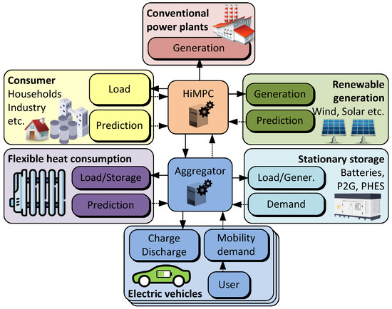
Figure 1.
Architecture of the energy management system featuring a Hierarchical Model Predictive Control (HiMPC) framework. The HiMPC integrates conventional and renewable power plants, consumers, and stationary storage systems such as batteries, power to gas (P2G) with reconversion via fuel cells, and pumped hydro electric storage (PHES), as well as electric vehicles. Arrows indicate the flow of information, with renewable generation, consumer load, and the charging/discharging power of electric vehicles directed into the HiMPC for processing. The HiMPC generates control signals to manage conventional generation, electric vehicle power, storage operations, and the curtailment of volatile renewable energy sources. An aggregator simplifies this complexity by distributing control signals to individual vehicles and consolidating measured and predicted data.
MPC has been shown to handle multi-timescale coordination and sector-coupled flexibility effectively [12,13,14,15,16,17,18,19,20,21,22,23,24]. To illustrate the framework under stringent conditions, we include a single zero-exchange (autarky) run; prior work treats autarky as a conservative endpoint that usefully reveals domestic adequacy and flexibility needs when cross-border support is unavailable [25,26,27,28,29,30].
The methodology section is organized into two main sections: the HiMPC framework and the Energy System’s Components and Parameterization. In the model’s framework, the outer MPC (referred to as Level 1 in the following) is responsible for maintaining power balance with a 15-min sampling time and utilizes forecast data for 24 h to determine optimal setpoints. The inner MPC (designated as Level 2) operates with a 1-s sampling time and focuses on short-term frequency regulation to ensure system stability. All zones are interconnected to maintain equilibrium and balance power distribution across the system. The second section focuses on defining the system’s components and their parameterization, providing a comprehensive overview of their operational constraints and limitations.
2.1. HiMPC Framework
The objective of frequency stabilization is to maintain the target grid frequency of 50 Hz by ensuring a balance between power generation and consumption. This process is divided into primary, secondary, and tertiary control, which are differentiated by their response times and specific functions. Although traditional frequency regulation methods are effective for systems with large, centralized power plants, they can cause instability in systems dominated by small, decentralized units and highly variable renewable energy sources, which is primarily due to the diminished stabilizing effects of rotating masses. The heightened instability and the inherent variability of wind and photovoltaic power require more rapid response times for power adjustments [32,33,34].
To model frequency dynamics, an equation is required to capture the interdependencies between grid frequency, loads, and power plant characteristics, beginning with the derivation of the linearized dynamics of the generators’ oscillations, which are represented by
In this equation, denotes the deviation from the nominal frequency, , while H represents the absolute inertia constant, is the absolute nominal power, and refers to the absolute mechanical power of the generator. The load power is denoted as .
We adopt a lossless transmission approximation: ohmic line losses and reactive-power effects are neglected, and each control zone is modeled as a copper plate with power balance enforced on net exchanges rather than detailed AC power-flow equations. This isolates the controller’s behavior and keeps the optimization tractable; incorporating losses and network constraints is deferred to future work. The oscillation equation indicates that only power changes, and , are pertinent to frequency-stabilizing control. When these changes are perfectly balanced, no frequency deviation occurs. Ideally, any load variation should be compensated by a corresponding adjustment in generation, underscoring the critical importance of maintaining power balance for frequency stability.
Deriving a frequency model involves incorporating frequency-dependent loads, which introduces additional terms, resulting in
Here, the frequency dependency of the system’s loads is described by and , both of which vary with load dynamics; the former represents the loads’ damping, while the latter accounts for the kinetic energy of the generator’s rotating masses. Based on this, the state-space model is derived as
with the parameters
In this form, reflects the effect on frequency deviation, whereas relates to both power generation and load consumption, with the inertia constant H being computed as
It is assumed that conventional power plants have an inertia constant of and wind turbines have [33]. Based on findings in [34,35] among others, it is suggested that new variable-speed wind turbines contribute to grid stabilization by increasing their rotational inertia. Assuming that the wind turbines in the considered future scenario possess this capability, the constant of the relevant power of the wind turbines is approximated using the average power over the simulated period. For the power plant capacity, the total nominal power is used, which includes the base load, medium load, and peak load, as determined by
The damping coefficient for frequency-dependent loads, , suggests that load variations typically range from 0% to 2% for each 1% change in frequency and can be approximated using
as proposed by Andersson [36]. In simulations involving a single zone, remains constant; however, it can vary across different zones and simulation scenarios.
2.1.1. Power System Setup
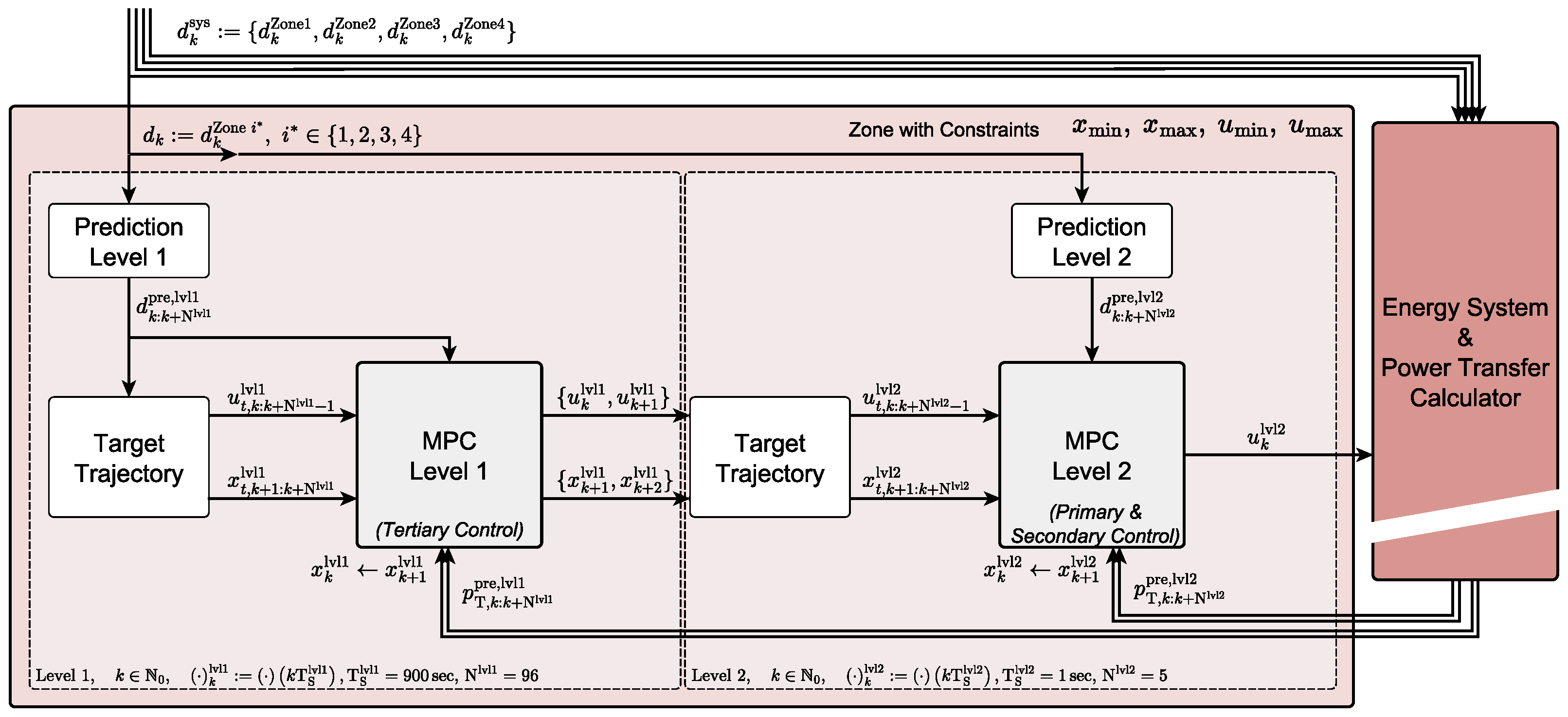
Figure 2 depicts the fundamental architecture of the HiMPC employed in this study, outlining the control strategy for a single control zone while preserving the traditional division into primary, secondary, and tertiary controls typical of classical frequency regulation.
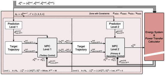
Figure 2.
Hierarchical cascaded Model Predictive Control (HiMPC) for one control zone. Level 1 is a slow supervisory MPC that optimizes 15-min reference setpoints over a day-ahead horizon subject to unit and network constraints; in classical terminology, this corresponds to tertiary (manual frequency restoration) control. Level 2 is a fast regulatory MPC that combines (i) droop-like action to stabilize the frequency after sudden disturbances—analogous to primary control—and (ii) an integral correction that drives the steady-state frequency error toward zero within actuator limits—analogous to the dynamic part of secondary control. Thus, Level 2 covers the roles of primary and secondary regulation, while Level 1 provides the slower tertiary scheduling. The assignment to classical frequency control is given in parentheses in the diagram. All four control zones share the same architecture but differ in parameterization. They are coupled through the Energy System and Power Transfer Calculator. Each zone follows the structure shown in the salmon-colored box, comprising two MPC layers.
Level 2 MPC combines primary and secondary control. It runs at a 1 s sampling time with a 5 s prediction horizon. The fast loop applies a droop-like action proportional to the instantaneous frequency deviation to arrest transients (primary role) and, in parallel, an integral correction that drives the steady-state frequency error toward zero within actuator limits (secondary role). A sampling time of 1 s is intentionally coarse; sub-second sampling on the order of a few hundred milliseconds or less would better suit low-inertia conditions. An optional intermediate third layer with a sampling time of a few tens of seconds can further smooth corrections between the 1 s loop and the 15-min scheduler. We keep 1 s/5 s here to limit runtimes; for the types of questions this framework is intended to support—e.g., storage sizing, ratios of storage power to plant capacity, and sensitivity to forecast quality—this simplification does not limit its applicability, although we do not perform those analyses here.
Level 1 MPC provides tertiary control. Fast frequency dynamics are not represented at this layer. Instead, Level 1 optimizes the power balance on a 15-min grid over a 24-h horizon, embedding forecasts and slower plant dynamics such as ramp-rate limits, start-up trajectories of power plants and electrolyzers, and storage charging/discharging constraints. Every 15 min, it issues setpoints for dispatchable units, storage, and sector-coupled loads. A trajectory generator converts these piecewise-constant setpoints into smooth second-scale reference trajectories for Level 2 to prevent steps at the layer interface. In effect, Level 1 pre-positions flexibility (charging, curtailment, commitment) while Level 2 closes the fast frequency loop.
The hierarchical formulation embeds all variables in constrained optimizations. The state vector contains controllable power outputs and storage states; the input vector represents commanded ramp rates; disturbances cover uncontrollable injections and withdrawals (wind, photovoltaic, and demand) with forecasts. Bounds on states and inputs, together with tracking of Level 1 references and frequency objectives, define the constraints and the cost function. Both layers operate in receding-horizon fashion: at each sampling instant, the respective MPC predicts over its horizon, solves the constrained problem, applies the first control move, and repeats with updated measurements and forecasts. Disturbances that occur just after a control update can cause larger excursions in low-inertia conditions when sampling is slow. The recommended mitigations are (i) using a shorter, sub-second Level 2 sampling time, and/or (ii) inserting an intermediate layer with a sampling time of a few tens of seconds that relieves the 1 s loop from large setpoint steps; both are compatible extensions of the presented architecture.
Optimal control behavior is achieved by minimizing these total costs through an optimization process based on a continuous-time state-space model, which is described by
This mathematical framework comprises several key components: the state matrix , which governs the dynamics of the system states; the input matrix for controllable variables; and the disturbance matrix for external influences. The system output is determined by the output matrix , influenced by the state vector, and further affected by inputs through the feedthrough matrix and disturbances through . In general, these matrices can be time-varying (for example, effective inertia depends on the operating point); to keep the computational burden manageable, we freeze them within this study, which is adequate for the capacity-sizing or adequacy-planning questions addressed by the proposed framework.
The continuous dynamics are converted into a linear model and discretized with the respective sampling time of each layer ( for the fast layer, for the scheduler; an optional intermediate layer could use ) to make them suitable for the control algorithm. The discretization enables the controller to evaluate the system’s behavior at each time step k, leading to
where future states and outputs are determined based on current states, inputs, and disturbances. The subscript indicates the discrete form of the matrices used in this formulation.
2.1.2. Optimization Problem Setup
To compute the optimal solution, an optimization algorithm is required. In this work, the FORCES solver [37] is used, which employs interior-point methods well suited for linear quadratic problems. The state-space model, previously introduced, is reformulated as a quadratic programming problem to enhance computational efficiency and structure. This formulation minimizes a cost function J over a prediction horizon , taking into account system states , inputs , and disturbances , which is formulated as
s.t.
ensure that the system states and inputs remain within predefined bounds, the initial state matches the current system state , and that the system dynamics are respected as per the given equations.
The objective function minimizes the deviations of the system states, , and control inputs, , from their reference trajectories, while also accounting for the impact of disturbances . The terms , and their cross-product terms represent the weighting matrices that define the importance of different states, inputs, and disturbances in the cost function. These weights assign priorities to the optimization variables based on their relative importance to the system’s overall performance. The optimization variables are normalized componentwise by their maximum absolute value; accordingly, the state-related weighting matrices are defined on the normalized states, while input and disturbance channels are handled via dedicated scaling matrices. The terminal cost guarantees system stability with the matrix obtained by solving the discrete-time algebraic Riccati equation over an infinite horizon. In this formulation, it is assumed that , as the interaction between states and inputs is not weighted, and the discretized cost function matrices are predefined.
Optimization solvers designed for sparse representations offer superior scalability relative to those tailored for dense forms. This advantage is particularly evident as complexity grows and the prediction horizon extends, enabling shorter computation times when utilizing the sparse form [38]. To convert the optimization problem, given in (12), into its standard form, the vectors and matrices are initially stacked into a sparse form, leading to
where the number of diagonally entered matrices in and equals . However, in this configuration, the matrix is excluded to prevent it from overly affecting the control with a shorter prediction horizon; the weighting matrix is used instead. For the equality constraint in sparse form,
with the matrices
that may evolve gradually over time to account for changes in the system, such as the availability of storage through vehicle-to-grid integration. These adjustments are reflected by indexing the matrices, ensuring the optimization process adapts to the system’s dynamic conditions. This can then be rearranged to conform to the format required by the optimization solver, resulting in
The system boundaries are modeled as inequality constraints and arranged into a suitable stacked format, resulting in
with
that can be compactly expressed using the identity matrix in the appropriate form
By rearranging and eliminating terms independent of the optimization variables, the discretized cost function, as shown in (12), simplifies to
with its equality and inequality constraints defined in (17) and (20) forming its standardized structure, which is suitable for the FORCES solver.
The optimization framework is extended to include the system’s outputs, represented by the vector , in a manner that enables more precise control over power generation. By appropriately weighting these outputs, the power levels in the state vector are aggregated through the matrix , allowing for a weighted balance of the system’s overall power balance, which is critical for frequency regulation. As a result, the optimization focus is shifted to the outputs in the following steps. Deviations from the setpoints, noted as , are incorporated using the weighting matrix . With the setpoints for the outputs defined as , the formulation is given by
yielding the cost function to
or in its standardized form to
with
Based on the transformation in (24) and considering the symmetry of , the equations can be calculated as
Following a thorough process of these reformulations, the cost function presented in (21) is finally obtained in its restructured form as
with
2.1.3. Structure of the HiMPC’s Outer Layer
HiMPC’s Level 1 provides tertiary control only; primary and secondary regulation are handled entirely by Level 2. Level 1 performs slow, anticipative scheduling to keep the zone energy balanced, but it does not model fast frequency dynamics. The same continuous-time state-space structure is used for all control zones and is discretized at 15 min, matching forecast granularity and operational scheduling intervals. The prediction horizon spans 96 steps (24 h). Every 15 min, Level 1 optimizes setpoints for dispatchable plants, storage, and sector-coupled loads under ramp-rate, start-up, and state-of-charge constraints; a trajectory generator then maps these setpoints to smooth second-scale references for Level 2. The Level 1 model uses 15 states, , representing aggregated generation, storage, and controllable demand, and it is given by
The control inputs, denoted by , represent the changes in electrical power and consist of a total of 11 input variables, and these are described as
Moreover, the system is affected by 5 external disturbances, denoted by , which capture exogenous disturbances—such as renewable generation and load demand—that are beyond the system’s control. These disturbances are formally expressed as
With the model’s variables introduced, the system’s state change, as governed by (8), can be expressed for the continuous case as
where is the system matrix, is the input matrix for controllable variables, and is the input matrix for disturbances. In Level 1, these matrices are constant, eliminating the need for time-step indexing. Upon discretization of the system matrices, denoted by the additional subscript d, the expression for the subsequent system state is derived from (10). The system outputs, formulated as in (11), are obtained directly from the discrete state-space model, with the power balance being accounted for, ultimately yielding the expression
with
resulting in a total of 16 outputs.
2.1.4. Structure of the HiMPC’s Inner Layer
Level 2 combines primary and secondary control. It extends the Level 1 model by explicitly including the frequency deviation from the 50 Hz nominal and by treating inter-zonal tie-line power as an external disturbance. Level 2 tracks the reference trajectories delivered by Level 1 and, on top of these, applies fast corrections: a droop-like term proportional to arrests transients (primary role), while an integral term drives the steady-state frequency error toward zero within actuator and ramp-rate limits (secondary role).
The sampling interval is 1 s with a 5 s prediction horizon. This choice is intentionally coarse for computational efficiency; sub-second sampling (on the order of a few hundred milliseconds or less) would better suit very low-inertia conditions. As already mentioned, we retain 1 s/5 s in this study to manage runtimes and because the aim is to present a reusable framework; detailed sub-second design is left for future work.
In total, the Level 2 model uses 16 states, 16 outputs, 11 inputs (unchanged), and 6 disturbances. The continuous state-space formulation reuses the Level 1 asset dynamics and augments them with the frequency channel and the tie-line power disturbance, resulting in
with the matrices
whose components are derived as shown in (4). The outputs at Level 2 are equivalent to its states , leading to
with
2.1.5. Coupling of Control Zones
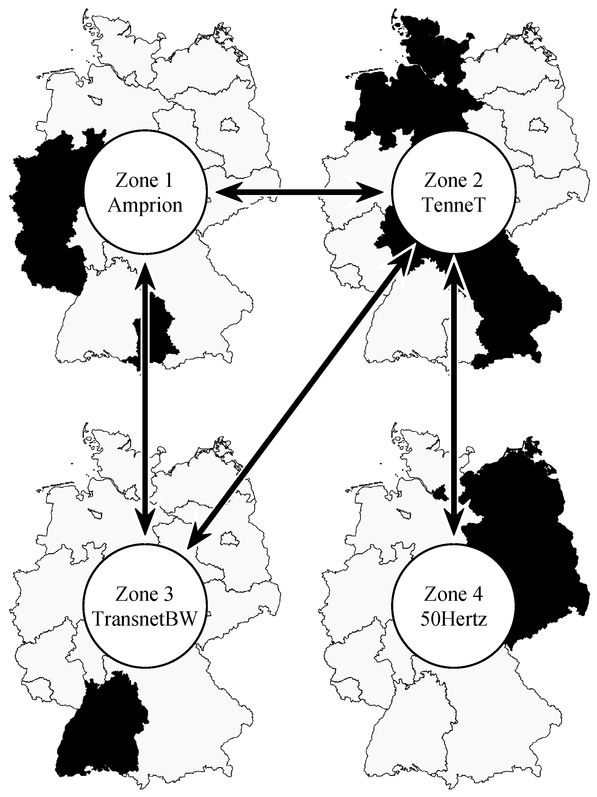
In this section, the modeled coupling of control zones is elaborated. Figure 3 provides a schematic representation of the transmission lines linking the power system’s zones, assuming that direct connections are limited to adjacent regions.

Figure 3.
Schematic representation illustrating the interconnections between the control zones of Germany’s transmission system operators: Amprion, TenneT, TransnetBW, and 50Hertz. The arrows indicate bidirectional power flows based on geographical locations. The black area in each map of Germany represents the respective coverage area of each control zone. Cross-border connections are not considered in this paper; the focus is solely on power exchanges occurring between the zones.
Based on these interconnections, the system can be formulated as
with the aggregate transfer power between Zones i and j computed by rearranging the equations to form
where is the Moore–Penrose inverse (pseudoinverse) of matrix .
However, the simulation model does not require the exact specification of transfer powers, since these values are inherently determined by the state-space model of the system as a whole. The total transfer power for each zone is integrated as part of the predicted disturbance variables, thus falling outside the direct influence of the MPC. For instance, the transfer power between Zone 1 and Zone 2 is automatically accounted for by
where X represents the reactance of the line, and and correspond to the phase angles [24]. For small changes, the voltages and can be assumed constant, leading to
or
with
When a higher-level control system calculates transfer powers, any change in the desired transfer power can cause individual zones to experience frequency shifts or differences in frequency between them. According to (41), these changes require the actual transfer power to be adjusted to match the new conditions. To maintain system stability, the sum of all transfer powers must be zero, balancing out any frequency deviations with the power exchanged between zones. In scenarios with interconnected zones, the Level 1 MPC compensates for transfer power adjustments by modifying the power balance term . In contrast, the Level 2 layer addresses these adjustments through the disturbance variable as specified in (33).
To precisely account for the coupling effects, transfer powers are incorporated into a state-space model representing the entire energy system. The comprehensive model encompasses state-space representations for all zones along with their interconnections illustrated in Figure 3. The matrix represents the continuous system matrix of the Level 2 MPC for a specific zone i, where unoccupied positions are represented by zero matrices. The complete continuous state-space matrix , which incorporates the couplings between zones, is denoted as
with
where is the factor of Zone i, and denotes the power constant between Zones i and j, as assumed in this model, with the corresponding values provided in Table 1. Since transfer power is already considered as a disturbance in matrix , the input and disturbance matrices
can be taken and extended so that the entire state-space model
results. The state vector now includes the state vectors of Zone i and the transfer powers, such that
The configuration of the continuous system matrix and its discretized counterpart illustrates that the transfer power coefficients and are set to zero. The structure of the discretized matrix highlights that the frequencies of the zones are mutually dependent and are affected by all power levels relevant to frequency. For instance, a decrease in power generation in Zone 1 will cause a frequency drop in all interconnected zones. This interdependence is crucial when defining target frequencies.
2.1.6. Reference Trajectories
Establishing reference trajectories allows for the regulation of MPC behavior, which is analogous to the role of tertiary control in conventional frequency regulation. The MPC minimizes deviations from these reference points to optimize performance and reduce costs.
The method for determining scheduled transfer powers is introduced first. These transfer powers are required to be as smooth as possible, ensuring an equitable distribution of wind and photovoltaic power generation proportional to the consumption levels across zones. The objective is to ensure that all zones meet their electricity demands equally from variable renewable energy sources. This calculation is based on the moving average, which is defined as
where represents a discrete data point at time step k, and is the number of neighboring data points on either side of . With , the time span considered is time steps, covering both past and future points. This moving average accounts for a full day using the available signal. Since the prediction horizon of the Level 1 MPC is 96 time steps, the moving average for the next 96 steps is computed using data from the past 12 h and predicted data for the upcoming 36 h (or time steps).
At each time step, the moving averages for photovoltaic power , wind power , and power demand for all four zones are determined. These values are then used to calculate the desired transfer power
with
and the power balance trajectory being determined by
Using moving averages ensures a smooth transfer of power between zones, which is based on average renewable energy generation and consumption. Next, the trajectories for base-load power plants and mid-load power plants are calculated as
with the respective shares of the total power of these plants
Since the computed setpoints can exceed the power plant capacities, measures are taken to keep the trajectories within the defined power range.
The Level 2 MPC receives reference trajectories generated by Level 1 and applies fast corrections around them. In the 2045 scenario, fuel cells and electrolyzers are modeled to follow operational trajectories analogous to those of base-load and mid-load power plants. Setpoints for electrolyzers are determined by surplus power availability. However, adhering to these trajectories often results in the simultaneous operation of both fuel cells and electrolyzers by the MPC. Prioritizing the operation of electrolyzers is crucial, as their smoother functioning is more favorable from both economic and technical perspectives [39]. Nonetheless, achieving this may require the concurrent operation of other generators, such as fuel cells and gas power plants, potentially leading to greater energy losses. Maintaining system stability becomes particularly challenging during periods of high variability in renewable energy output.
Battery power is not predefined, as leaving it unconstrained allows for the greatest flexibility in the optimization process. Providing a reference trajectory for the state of charge is generally sufficient. The reference trajectories for Level 2 are modeled using spline interpolation between previous and updated target values, resulting in a smooth setpoint profile that minimizes frequency peaks.
A unique case arises in the prediction of transfer power, which is treated as a disturbance in the Level 2 layer of each zone and is only indirectly specified by the Level 1 MPC, as it is incorporated into overall power balancing. Achieving a smooth frequency response necessitates an even setpoint profile for transfer power. Sudden changes in the power slope must be avoided, as they induce frequency spikes according to (2). To address this, a cubic polynomial is used to define the trajectory.
The setpoint for frequency deviation is set to zero, which in isolated systems operating in island mode typically leads to rapid frequency stabilization after power disturbances, ensuring high control performance. However, this approach can present challenges in interconnected systems. A comparison of the continuous system matrix with the discretized system matrix for the entire system shows that the frequency in a coupled zone is influenced by the power outputs and frequencies of other zones. These interdependencies are not accounted for in the MPC state-space model for individual zones, making it incapable of detecting events occurring in other zones. Consequently, in the event of a frequency deviation, all zones may attempt to correct it simultaneously, leading to overcompensation and the onset of frequency oscillations.
According to (41), the change in transfer power depends on the difference in frequency deviations and between two zones. Consequently, high control accuracy of the frequency is essential to achieve balanced transfer power. However, a small frequency difference is necessary to adjust the transfer power effectively. If the frequency deviations of the zones converge to zero too rapidly, it may hinder the adjustment of the transfer power. To address this, the Level 2 MPC is provided with a reference trajectory for frequency, which gradually reduces the deviation over time steps in a linear manner. Two important factors must be taken into account: the weighting of the frequency, as relative costs decrease as the deviation from the target frequency lessens, and the potential for a slower compensation of load disturbances. In this model, a time of s was selected, ensuring that the frequency deviation is fully compensated within the prediction horizon of Level 2.
2.1.7. Simulation Setup
The energy model simulation was conducted in MATLAB/Simulink R2024b. Figure 2 shows a simplified schematic of a single zone with the HiMPC framework. While the structure is the same across all zones, each zone has unique parameter configurations. The blocks represent functional subsystems, and arrows depict the flow of information and control signals throughout the model.
Before starting the simulation, load profiles, reference trajectories, and dynamic constraints are initialized via a script, covering both prediction data and actual generation and consumption. The prediction block provides profiles based on current disturbances and computes average values for trajectory and transfer power calculations, which influence the dynamic constraints and MPC setpoints. The Level 1 MPC calculates the setpoints for the states and inputs , which are passed to the trajectory generator. This generator smooths the setpoints through interpolation and forwards them to the Level 2 MPC. Transfer power trajectory calculation is performed outside the zone’s subsystem. The Level 2 MPC generates control signals based on setpoints, accounting for frequency, which are then used by the energy system.
Within the energy system block, the response to disturbances and control signals is computed and relayed back to the cascaded MPC through the state vector, closing the control loop. The model in Figure 2, along with the state-space representations for both control layers, is used to evaluate zone behavior in isolation, assuming zero transfer powers.
Daily moving averages of wind, photovoltaic generation, and consumption are provided to the transfer power calculator, which returns setpoints for the transfer powers. Using these data, each zone’s HiMPC computes control signals (input vector ) for power adjustments within the zone and sends them to the energy system calculator. The energy system considers inter-zone couplings, updates the system state, and feeds the information back to the control loop.
The structure of the continuous system matrix and its discretized form highlights the interdependence of frequencies between zones and their connection with frequency-related power variables. A reduction in power generation in one zone causes a frequency drop across all zones, requiring precise target frequency settings. To prevent abrupt frequency changes, the target transfer powers must be carefully adjusted.
2.2. Components and Parameterization
This section details the components of the energy system and their parameterization for a forward-looking 2045 testing scenario. It specifies capacity constraints, ramp-up characteristics, and operational dynamics for conventional power plants, vehicle-to-grid, electrolysis, fuel cells, and load management via heat-storage systems. The scenario adopts NEP Scenario A [31], which projects a substantial rise in electricity demand and a major build-out of renewable and hydrogen infrastructure. Table 1 summarizes the key parameters used in the simulations.
2.2.1. Disturbances and Prediction Data
The accurate modeling of electrical load, wind, and photovoltaic generation requires high-resolution data for both real-time values and forecasts. In the HiMPC framework, actual performance values are incorporated via the disturbance vector , while predictions are handled through . The variable allows for the curtailment of fluctuating renewable energy generation. Intra-day forecasts are primarily used for wind and photovoltaic generation predictions, and in cases where actual values are missing, day-ahead forecasts are employed with gaps filled by linear interpolation.
In the Level 1 system, prediction data are updated at each time step, gradually adjusting the forecast over a 5-h horizon to align with the original prediction. The Level 2 MPC operates with a shorter prediction horizon of 5 s, assuming that measurable disturbances remain constant within this period, except for transmission power predictions, which are handled separately.
2.2.2. Power Plants
Conventional power plants play a significant role in today’s energy system and partially remain key as gas-fired plants powered by hydrogen from surplus renewable energy in the future scenario. For the MPC calculations, the constraints imposed by maximum power output and the duration of ramp-up and ramp-down processes are particularly relevant. The calculation of power plant output is derived from the rate of change in power within the continuous state-space model with the simplified assumption that
applies. Due to the large capacities in the control zones, dynamic ramp-up and ramp-down processes are not considered in the model.
The model simplifies plant classification by operational role—base-load, mid-load, and peaking power—based on ramp-up speed limitations [40,41]. Each plant category has specific ramp-up times, which are detailed in Table 1.

Table 1.
General model parameters for simulation. These parameters apply uniformly across all zones and include operational ramp-up times, power transmission coefficients, network parameters, efficiency factors, and battery state-of-charge (SOC) limits.
Table 1.
General model parameters for simulation. These parameters apply uniformly across all zones and include operational ramp-up times, power transmission coefficients, network parameters, efficiency factors, and battery state-of-charge (SOC) limits.
| Symbol | Parameter | Value | Source |
|---|---|---|---|
| Base-load plants ramp-up time | 3 h | [40,41] | |
| Mid-load plants ramp-up time | 2 h | [40,41] | |
| Peaking power plants ramp-up time | 15 min | [40,41] | |
| Shut down of volatile RE | 60 s | - | |
| Battery ramp-up time | 2 s | - | |
| Electrolyzer ramp-up time | 2 h | - | |
| Fuel cell ramp-up time | 2 h | - | |
| Pumped hydro electric storage ramp-up time | 5 min | [42] | |
| Flexible loads ramp-up time | 2 s | - | |
| Power Transmission Coefficients | |||
| Connection between Zones 1 and 2 | 533 MW | [36] | |
| Connection between Zones 1 and 3 | 533 MW | [36] | |
| Connection between Zones 1 and 4 | 0 MW | - | |
| Connection between Zones 2 and 3 | 533 MW | [36] | |
| Connection between Zones 2 and 4 | 533 MW | [36] | |
| Connection between Zones 3 and 4 | 0 MW | - | |
| Network Parameters | |||
| Minimum frequency deviation | Hz | - | |
| Maximum frequency deviation | 0.2 Hz | - | |
| Nominal frequency | 50 Hz | - | |
| Inertia constant of power plants | 5 s | [33] | |
| Inertia constant of wind turbines | 3.5 s | [33] | |
| Kinetic energy of rotating loads | 0 J | - | |
| Efficiency Factors | |||
| Battery charging efficiency | 0.97 | [43] | |
| Battery discharging efficiency | 0.98 | [43] | |
| Electrolyzer efficiency | 0.95 | [44] | |
| Fuel cell electrical efficiency | 0.60 | [45] | |
| Pumped hydro electric storage charging efficiency | 0.90 | [46] | |
| Pumped hydro electric storage discharging efficiency | 0.90 | [46] | |
| Normalized Battery SOC Limits | |||
| SOCmin | Minimum SOC | 0.2 | - |
| SOCmax | Maximum SOC | 0.9 | - |
For the 2045 simulation, it is assumed that the existing run-of-river, biomass, and pumped-storage capacities will remain in their respective zones. Fossil fuel plants will be phased out except for a small number of gas-fired plants using hydrogen. A modest expansion of pumped-storage capacity, as outlined in the NEP, will be distributed proportionally according to each control zone’s annual electricity consumption. The modeling parameters for these plants are detailed in Table 2.

Table 2.
Zone-specific model parameters for the year 2045 based on Scenario A of the Network Development Plan (NEP) [31]. The table presents the maximum power, storage capacity, peak power, energy demand, and minimum power values for each zone (Z).
2.2.3. Electric Vehicles and Batteries
In this study, electric vehicles are considered for grid stabilization to mitigate short-term fluctuations. The model, based on the work of Kennel et al. [24] and others [47,48], uses a driving profile and focuses on private vehicles for vehicle-to-grid services due to differing usage patterns.
Battery storage systems, including both stationary units (ranging from small-scale to large-scale) and electric vehicle batteries, rely heavily on the latter, which contribute 77% of the total storage capacity when fully integrated with Vehicle-to-Grid services. To reduce the computational complexity of the MPC, all grid-available storage systems are aggregated. The distribution of capacity and power across the zones is proportional to the total electricity consumption specified in the NEP [31].
As shown in Table 2, the model assumes two trips per day per vehicle, starting at 90% state of charge. After each trip, vehicles are unavailable for vehicle-to-grid services for one hour.
Dynamic limitations of battery storage and the energy used by electric vehicles are modeled as disturbances for each zone, handled by the Level 2 MPC, using interpolated one-second profiles. The model also includes constraints on minimum and maximum power levels and power change rates, which are all proportional to state of charge. A simplified linear battery model is used (see matrix in (30)), excluding processes like self-discharge and capacity loss. The state of charge limits are adjusted.
2.2.4. Electrolyzers and Fuel Cells
The modeling of electrolyzers and fuel cells in this study parallels the approach used for batteries, assuming a linear process where electrolyzers produce hydrogen, which is stored and later converted back into electricity using fuel cells. Installed capacities follow NEP’s Scenario A baseline and are incrementally increased in the simulation until electrolysis energy demand can be met domestically, yielding a self-sufficient system.
Ramp-up and heating times for electrolyzers range from minutes to hours, depending on the plant size and heating strategy [49], and must be limited to avoid accelerated cell degradation [39]. High-temperature fuel cells, such as solid oxide fuel cells, are also characterized by extended ramp-up times, which often require several hours to reach full operational conditions. To reflect real-world constraints, the model limits frequent startups and shutdowns, as these processes increase wear and reduce overall efficiency by extending the time required to reach steady-state conditions [50].
In the model, the combination of aggregated fuel cells, electrolyzers, and hydrogen storage addresses long-term supply–demand imbalances. Ramp-up times for these systems are set at two hours to account for the extended time needed to reach operational temperature and to prevent rapid fluctuations in operation. In the cost function, the hydrogen storage system’s state of charge is given a low weighting and is initialized at a low level. The simulation is mainly used to estimate maximum storage capacity and assess potential import needs or surplus generation. Detailed parameters are provided in Table 2.
2.2.5. Load Shifting with Heat Storage
Heat pumps coupled with thermal storage systems offer significant load-shifting potential, and they are modeled similarly to batteries and energy storage systems. The system combines limited thermal storage capacity with a disturbance that simulates heating energy demand, which depletes the storage and requires regular energy input to maintain balance.
Monthly average temperatures from 2022, provided by Deutscher Wetterdienst, were used to generate a temperature profile via cubic Hermite spline interpolation. Heating demand, , is derived by inverting this profile, assuming minimal demand at 15 °C. The ratio between minimum summer load and maximum winter load is based on the standardized W0 load profile for heat pumps [51] with the maximum load being 4.4 times the minimum. This scaling is then applied to the demand profile.
A load-shifting window of h is applied, during which the thermal storage is depleted according to the heating demand . The minimum storage level is set to zero, and the maximum storage level is determined as
Dynamic constraints on the storage level ensure that the aggregated heating load is fully met within the defined load-shifting window.
2.2.6. Weights
The weighting matrices within the control framework are instrumental in fine-tuning system behavior and prioritizing control objectives. Assigning high weightings to critically important variables ensures that deviations from their setpoints are minimized, while lower weightings indicate variables of lesser importance. However, when the use of a particular parameter is unavoidable—meaning the system must employ it regardless of associated costs—its weighting should be set disproportionately high to ensure it is appropriately managed within the optimization process. The specific values for these weightings were determined and refined through experimental simulations aimed at optimizing system performance. The primary goal was to minimize energy losses resulting from curtailing renewable energy generation and inefficiencies in charging and discharging operations.
Table 3 outlines the weightings assigned to power outputs and state-of-charge variables in the Level 1 controller, which were carried by matrix . High priority is given to maintaining the power balance, reflecting its critical importance for system frequency stability. Weightings for other variables are set relative to this benchmark, allowing for strategic flexibility or strict control as required.

Table 3.
Level 1 weights for power and state of charge (SOC) used in the simulations for 2045. The weights are summarized in matrix and within the optimization setup, and then they are applied to parameters such as the power balance, power plants, renewable curtailment, battery operations, electrolyzers, fuel cells, and storage systems.
Table 4 presents the weightings of the power change rates, which are the control inputs in the Level 1 controller and included in the cost function by matrix . Variables that require steady operation, such as base-load power plants and electrolyzers, are assigned higher weightings to discourage frequent changes, thereby promoting equipment longevity and system stability.

Table 4.
Level 1 weightings for power change rates used in the simulations for 2045. The weightings are summarized in matrix within the optimization setup, and then they are applied to various components such as the power plants, battery operations, electrolyzers, fuel cells, and flexible loads.
In the Level 2 controller, as shown in Table 5, weightings are assigned to both states and outputs with a focus on minimizing frequency deviations and adhering to the reference trajectories provided by Level 1. Here, the frequency deviation is given significant importance, and variables like the state of charge of batteries and renewable energy curtailment are weighted more heavily to ensure effective short-term frequency regulation.

Table 5.
Level 2 weightings for power and state of charge (SOC) used in the simulations for 2045. The weightings are summarized in matrix within the optimization setup, and then they are applied to parameters such as the frequency deviation, power plants, renewable curtailment, battery operations, electrolyzers, fuel cells, and storage systems.
3. Illustration of Framework Behaviour
This study demonstrates a Hierarchical Model Predictive Control (HiMPC) framework and illustrates its operation on Germany’s Netzentwicklungsplan (NEP) 2045 capacity projections under a strict zero-exchange (autarky) constraint. Existing research shows that HiMPC is effective for renewable-integrated power systems; here, we use a complete self-sufficiency setting as a stringent, policy-relevant illustration of the framework, highlighting how it coordinates sector-coupled flexibility with long-term storage without claiming a separate adequacy study.
The framework simulates Germany’s four transmission zones with a portfolio of energy assets, including variable renewables (wind, solar), semi-dispatchable generation (run-of-river hydropower, biomass), and multi-timescale storage technologies. Short-duration battery storage addresses intra-day fluctuations, pumped-hydro storage manages multi-day imbalances, and hydrogen systems (electrolysers paired with fuel cells) provide seasonal storage and reconversion. Dynamic power balances are enforced through flexible demand with asset coordination optimized across hierarchical layers: long-term scheduling at 15-min resolution to pre-position flexibility for prolonged low-renewables periods and 1-s control to maintain frequency close to nominal. This dual-timescale setup demonstrates the simultaneous handling of adequacy closure and operational stability within one architecture.
This section progresses through three phases. Level 1 simulations establish annual energy balance, locate capacity bottlenecks, and derive regulation power requirements in the zero-exchange case. Level 2 simulations use the setpoints supplied by Level 1 to illustrate controller behavior: three representative days (sunny, windy, low-renewable) show how storage, demand shifting, and setpoint tracking keep frequency near nominal in an isolated-zone setting, and a subsequent coupled-zone case demonstrates how inter-zonal transfers suppress frequency deviations. The third part exposes the system to unplanned events—extreme weather sequences, generation outages, and sudden load spikes—to illustrate how fast storage, demand shifting, and limited fuel-based units are coordinated by the hierarchy without resorting to load shedding.
3.1. Level 1
The Level 1 HiMPC simulations for 2045 instantiate and operate the NEP-projected generation, storage, and sector-coupled capacities under a strict zero-exchange setting to illustrate how the framework closes balances and pre-positions flexibility. Applying Scenario A parameters, power-balance calculations determine illustrative asset adjustments with storage state-of-charge monitoring identifying periods of surplus generation and domestic deficits.
Regulation-power shortfalls appear across zones, ranging from 0.7 GW in Zone 3 to 10 GW in Zone 1. To maintain balance within the example, we increase fuel-cell capacity accordingly, reflecting spatial disparities in renewable availability and demand. Zone 1 requires the largest uplift (+10 GW), followed by Zone 2 (+9 GW), Zone 4 (+6 GW), and Zone 3 (+1 GW), for a total addition of 26 GW. The resulting 49 GW fuel-cell fleet illustrates the role of hydrogen reconversion in covering residual load during prolonged low-renewables periods.
As shown in Figure 4, wind and photovoltaics provide 444 TWh (166 GW peak) and 375 TWh (255 GW peak), respectively. Run-of-river, biomass, and gas/pumped storage collectively supply 22 TWh, peaking at 8 GW. Battery systems discharge 118 TWh (74 GW peak) to manage short-term fluctuations, while electrolyzers convert 144 TWh (80 GW peak) of surplus electricity into hydrogen. Fuel cells subsequently reconvert 90 TWh (49 GW peak) of hydrogen back to electricity. Battery charging requires 179 TWh (127 GW peak), and electrolyzer operation demands 144 TWh, reflecting energy losses during storage cycles.
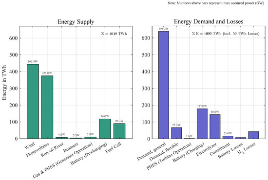
Figure 4.
Cumulative energy balance and storage losses for the 2045 autarky simulation under NEP’s Scenario A with maximum instantaneous power indicated above each bar. Energy flows include generation from wind (444 TWh, 166 GW peak), photovoltaics (375 TWh, 255 GW peak), run-of-river (8 TWh, 4 GW peak), biomass (4 TWh, 2 GW peak), and gas/pumped hydro storage (PHES) (10 TWh, 2 GW peak). Storage systems discharge 118 TWh via batteries (74 GW peak) and 90 TWh via fuel cells (49 GW peak), while electrolyzers consume 144 TWh (80 GW peak) for hydrogen production. Electromobility demand is met equally by direct battery charging and grid electricity. Storage losses (8 TWh for batteries, 42 TWh for hydrogen) reflect round-trip efficiency penalties during charging and discharging. Run-of-river power plants, biomass, and gas are modeled as base, medium, and peaking resources, respectively, within the hierarchical control framework.
Wind and photovoltaic curtailment totals 17 TWh (25 GW peak) to align generation with stability constraints. Storage losses amount to 8 TWh for batteries and 42 TWh for hydrogen systems. Despite these losses, 819 TWh of renewable generation is utilized, representing 99% of total production. A decline in hydrogen storage levels toward the end of the year coincides with reduced renewable output and elevated winter demand (Figure 5); in this illustrative setup, the system draws 13 TWh of hydrogen and requires a total storage capacity of 53.6 TWh to maintain balance.
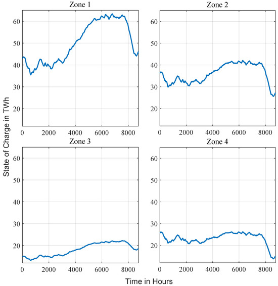
Figure 5.
State of charge (SOC) of the hydrogen storage system over the year 2045, highlighting periods of significant depletion, particularly at the end of the year.
Analysis of daily operational profiles for electrolyzers and fuel cells reveals distinct utilization patterns under the simulated zero-exchange conditions. The maximum installed electrolyzer capacity of 80 GW operates intermittently, while the 49 GW fuel-cell capacity exhibits more sustained operation. Annual full-load hours are 1810 for electrolyzers and 1844 for fuel cells, differing from NEP market projections of 4471 and 384, respectively. This reflects the higher volatility of residual load at high renewable penetration: electrolyzers track surplus episodes, whereas fuel cells provide extended coverage during low-renewables sequences, increasing their full-load hours and preserving the need for substantial output capacity.
The analysis of inter-zonal transfer performance builds on regional imbalances in generation and demand, quantified using the regulated load, which is defined as the residual load minus inter-zonal transfer power
where the residual load is given by
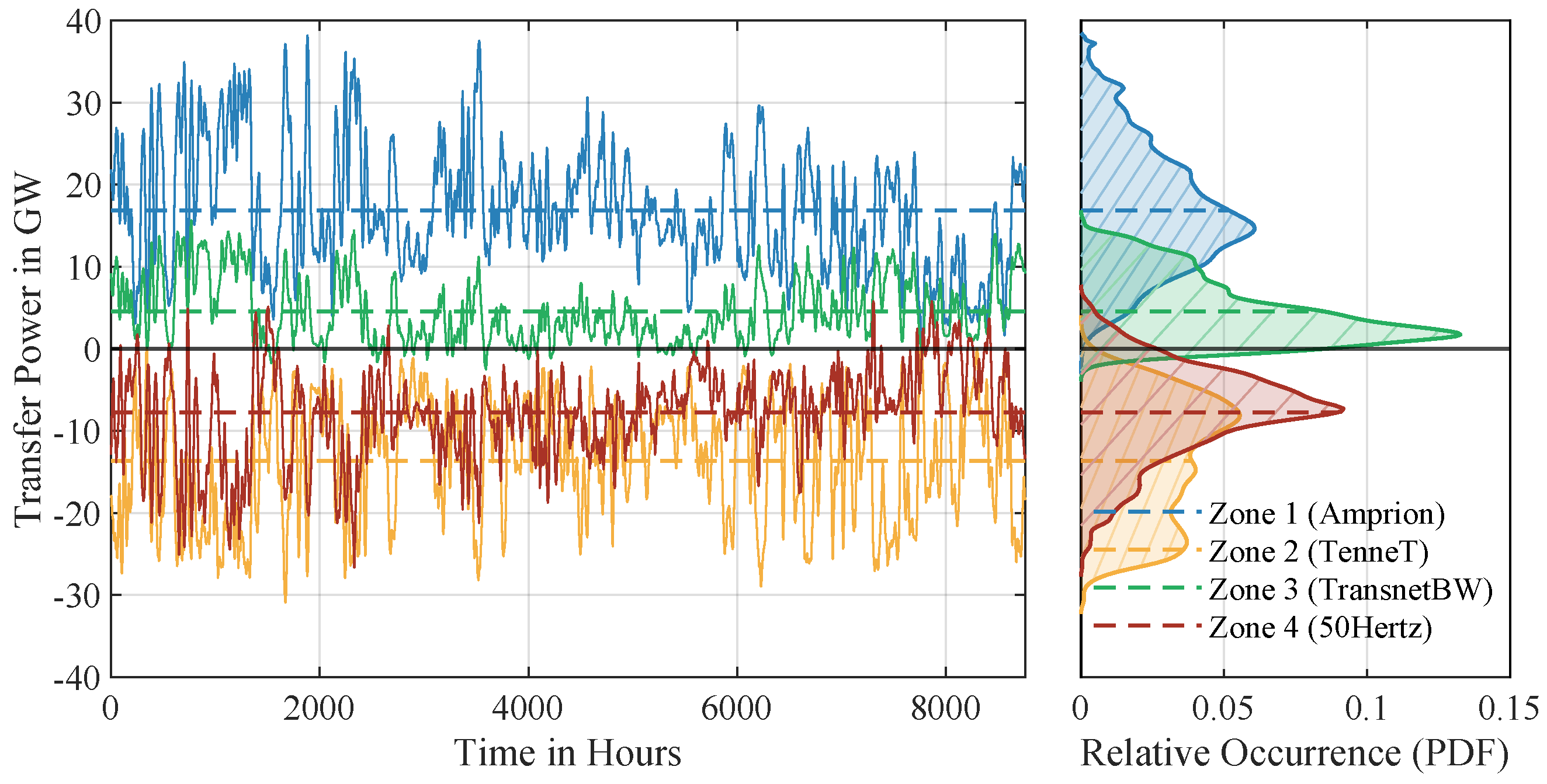
Here, represents demand, wind generation, and photovoltaic generation at time step k. The results reveal significant inter-zonal transfer requirements, with average transfer powers of approximately 17 GW in Zone 1, 14 GW in Zone 2, 5 GW in Zone 3, and 8 GW in Zone 4, as shown in Figure 6. Peak transfer capacities approach 39 GW, highlighting the substantial power flows needed to balance regional disparities in renewable generation and demand. The transfer power, reaching up to 39 GW, far exceeds the nominal ratings of individual high-voltage direct-current lines, which typically range from 1.5 to 3 GW, with some recent installations reaching 7.2 GW. Zone 1, with high wind generation, frequently exports surplus power, while Zone 3 relies heavily on imports due to lower renewable availability. To limit reliance on extensive grid reinforcement, a more balanced spatial distribution of renewables, targeted curtailment, and/or local hydrogen synthesis using excess energy provide alternative balancing options, allowing an economically feasible mix of curtailment, transfers, and storage.
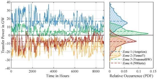
Figure 6.
Inter-zonal transfer powers across the four zones in the 2045 simulation. The blue line () represents the net power transfer of Zone 1 (Amprion), interacting with Zone 2 (TenneT) and Zone 3 (TransnetBW). The yellow line () corresponds to the net power transfer of Zone 2, interacting with Zone 1, Zone 3, and Zone 4 (50Hertz). The green line () indicates the net power transfer of Zone 3, interacting with Zone 1 and Zone 2, while the red line () represents the net power transfer of Zone 4, interacting exclusively with Zone 2. Positive values denote imports, and negative values indicate exports. Dashed lines represent the respective mean transfer powers for each zone. The right panel displays the corresponding probability density functions of the transfer powers with each zone’s mean marked by a dashed horizontal line extending to its density value. Data are recorded at a one-second resolution.
To illustrate the dynamics of balancing demand and supply, example weeks for a sunny, windy, and low-renewables period in Zone 1 are shown in Figure 7. During the sunny week, photovoltaic generation peaks at midday, reaching up to 50 GW, while battery storage discharges up to 15 GW in the morning and evening to cover generation gaps. Fuel cells operate at minimal capacity—primarily before and after the midday peak. The curtailment of excess solar output is minimal; most surplus is stored in batteries. In the windy week, wind generation fluctuates between 30 GW and 40 GW with occasional deficits requiring batteries to operate at an average output of 15 GW. Inter-zonal transfers peak at 25 GW, supplying power from other zones to compensate for renewable shortfalls. Curtailment is minimal, as wind generation aligns more consistently with demand. The low-renewables week shows minimal wind and solar generation: photovoltaic output remains below a few gigawatts, and wind averages about 20 GW. Fuel cells operate at high output during the last third of the week, averaging about 20 GW, while battery storage is depleted early. Inter-zonal transfers peak at 10 GW, supplying power to cover the prolonged shortfall. Curtailment is negligible due to the lack of renewable surplus, and conventional plants provide only limited support.
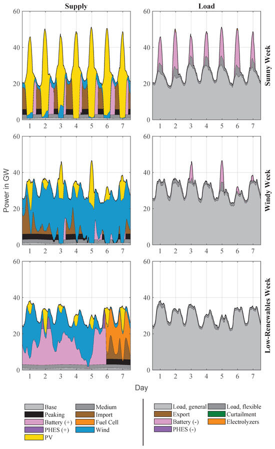
Figure 7.
Simulation results of power provision (left) and usage (right) for Zone 1 during exemplary sunny, windy, and low-renewables weeks in 2045. The sunny week shows pronounced photovoltaic generation peaks and compensatory battery discharging, the windy week demonstrates fuel cell operation and inter-zonal transfers during renewable deficits, and the low-renewables week highlights sustained fuel cell output and inter-zonal support during prolonged minimal generation.
3.2. Level 2
Level 2 simulations combine the Level 2 MPC layer with frequency modeling to illustrate system behavior under both isolated and interconnected configurations. In the isolated configuration, inter-zonal power exchange is zero, causing the residual load to match the regulated load directly. These simulations cover an entire year complemented by selected days (sunny, windy, and low-renewables) to illustrate diverse operational patterns in supply, load, and storage usage.
- Sunny Day (July)
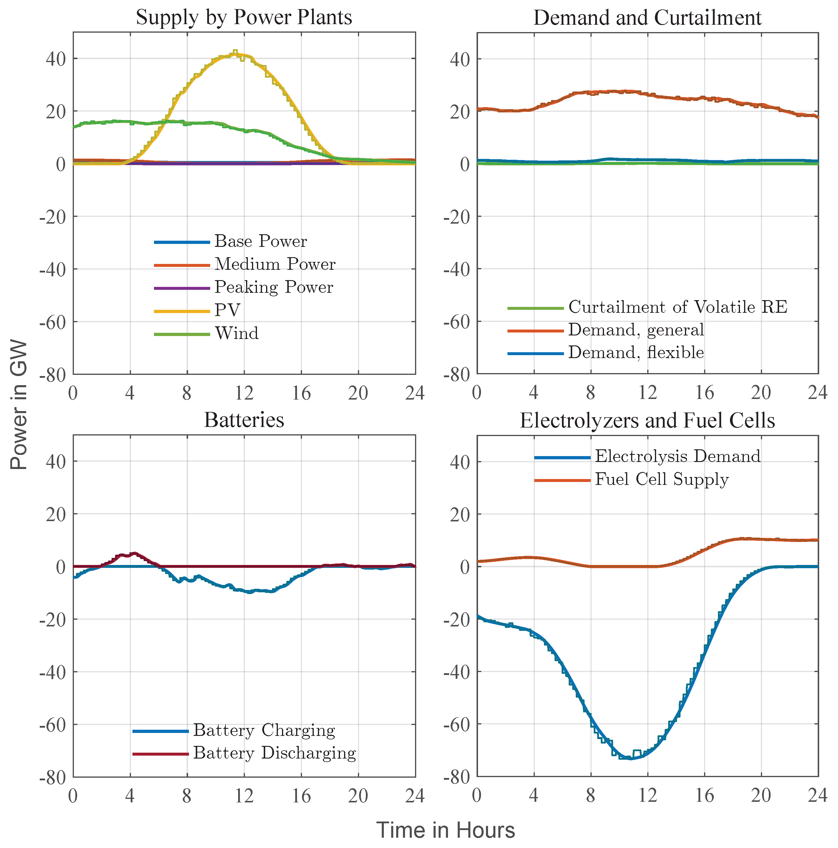
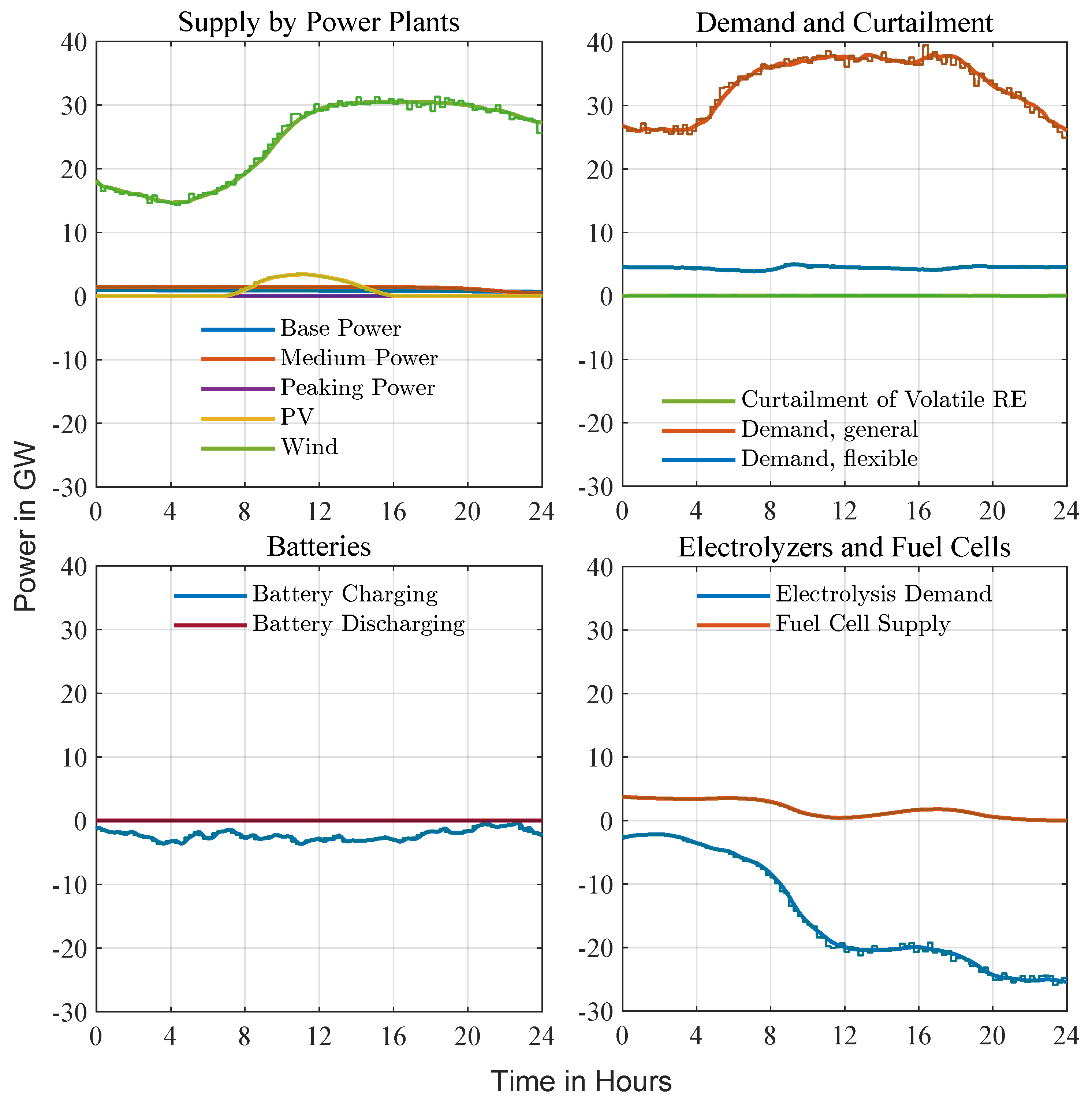
Figure 8 shows a July day with the year’s highest photovoltaic output in Zone 1. Stepped traces depict the 15-min Level 1 setpoints; smooth curves are the second-scale Level 2 trajectories. PV dominates the supply profile, pushing the residual load negative from late morning until mid-afternoon. To absorb this surplus, Level 1 schedules electrolyzer operation and net battery charging around the PV peak while prescribing modest battery discharge in the early-morning and evening shoulders. Wind provides a steady background contribution; base-, medium-, and peaking units remain at, or close to, their zero references for the entire day. General demand follows a broad daytime plateau, and the small flexible-demand trace indicates minor intra-day shifts executed by Level 2 for fine balancing. Curtailment appears only briefly when the battery state of charge nears its upper limit. Fuel cells stay idle until sunset, when they ramp gently to cover the rising evening load as PV output fades. Throughout the 24-h period, Level 2 keeps its smooth trajectory tightly within the stepped envelope, demonstrating that the hierarchy can track the day-ahead plan while managing sub-second variability.

Figure 8.
Sunny-day example (July, Zone 1). Strong midday photovoltaic production drives residual load negative. Level 1 pre-positions battery discharge around sunrise and sunset and enforces net charging at the PV peak; Level 2 refines these references, shifting flexible demand and applying brief curtailment as the battery state of charge approaches its limits. The hierarchy maintains frequency within a narrow band for the full 24-h period.
- Windy Day (February)
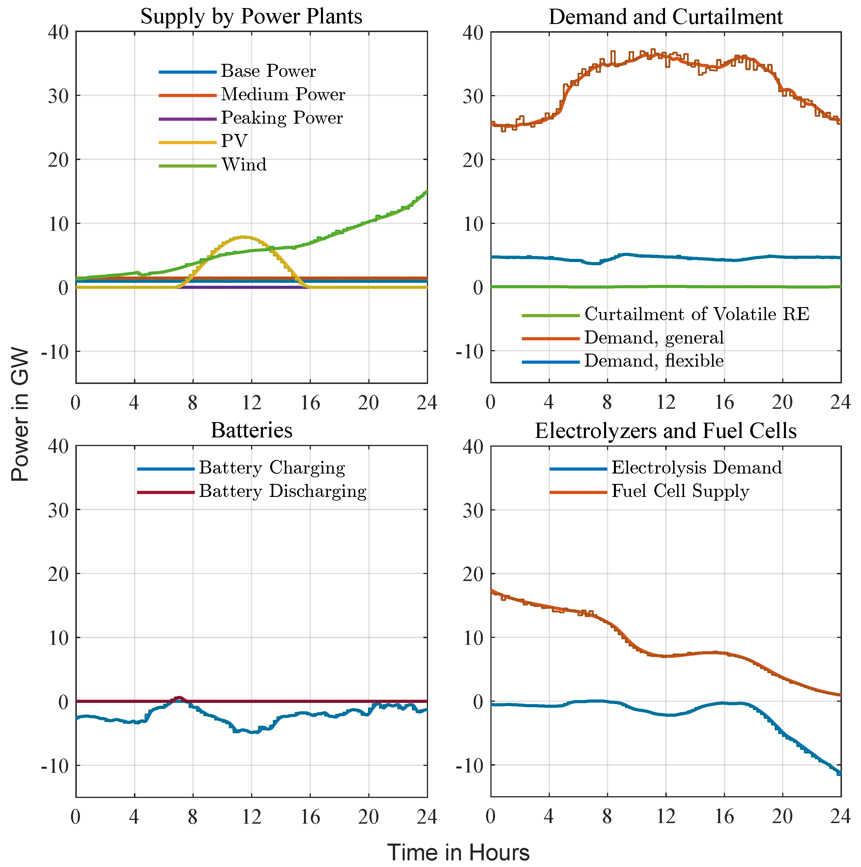
Figure 9 presents a February day with strong, variable wind in Zone 1. As in the sunny-day case, stepped traces indicate the 15-min scheduling layer and smooth curves the fast corrective layer; here, a February day with strong, variable wind in Zone 1 is shown. Wind dominates the supply stack and tracks its forecast closely, whereas photovoltaic output contributes only a modest midday pulse. Anticipating the surplus, Level 1 prescribes continuous battery charging and ramps electrolysis to its upper limit, keeping all conventional units at, or near, zero. Level 2 follows these setpoints and applies rapid adjustments when the wind trace deviates from the forecast, using pumped-storage and brief curtailment to absorb residual spikes. Fuel cells remain idling until the late evening, when they rise slightly to cover the load as wind eases. Throughout the day, the hierarchy maintains frequency deviations within a narrow band, demonstrating that advance electrolyzer scheduling and battery absorption are sufficient to balance a wind-dominated profile without calling on thermal generation.
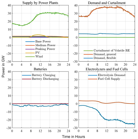
Figure 9.
Windy-day example (February, Zone 1). Stepped traces show Level 1 setpoints at a coarser interval, while smooth curves depict the second-scale Level 2 response. A highly variable wind profile dominates supply; Level 1 schedules electrolyzer demand and battery charging in advance, and Level 2 injects rapid corrections whenever actual output diverges from the forecast. Pumped storage and limited curtailment absorb residual spikes, and frequency remains close to nominal throughout the day.
- Low-Renewables Day (November)
Figure 10 shows a November day in Zone 1 when wind and solar remain suppressed for almost the entire 24 h. Stepped traces convey 15-min scheduling targets: fuel-cell output is kept near its upper reference from the early hours until midday and then ramped down as rising wind alleviates the deficit, batteries are assigned a shallow overnight discharge followed by cautious re-charging, and electrolyzers are switched off until a late-evening rise in wind allows modest hydrogen production. The smooth second-scale trajectories stay within those envelopes, with Level 2 discharging batteries before sunrise, trimming residual load peaks around noon, and replenishing charge once the brief PV pulse has passed. General demand follows its winter profile, while the flexible-demand trace shows only minor shifts—thermal storage is available but plays a small role because firm generation sets the margin. Curtailment is virtually absent, hydrogen SOC declines steadily through the deficit period, and conventional thermal units remain idle throughout. Frequency excursions stay well inside statutory limits, demonstrating that pre-scheduled fuel cells combined with strategically cycled batteries can bridge an extended renewable lull without calling on additional peaking generation or shedding load.
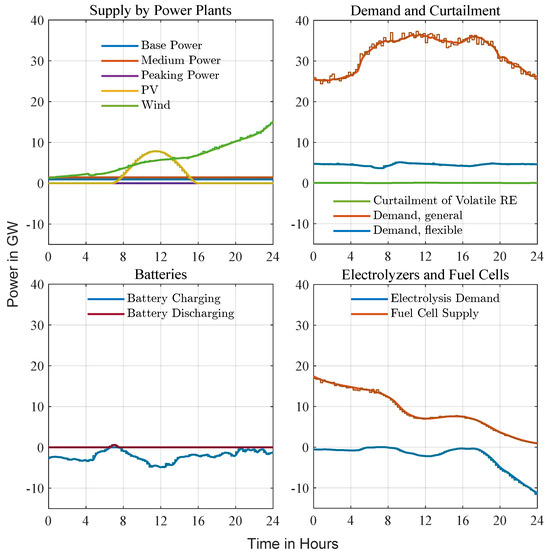
Figure 10.
Low-renewables example (November, Zone 1). With wind and solar contributions minimal, Level 1 commits fuel cells and peaking turbines near their upper bounds and schedules only a shallow battery cycle. Level 2 fine-tunes these stepped references, using batteries for balancing while electrolyzers remain idle and hydrogen storage gradually depletes. Despite the prolonged renewable deficit, frequency stays well within statutory limits, illustrating the framework’s ability to preserve adequacy when flexibility is scarce.
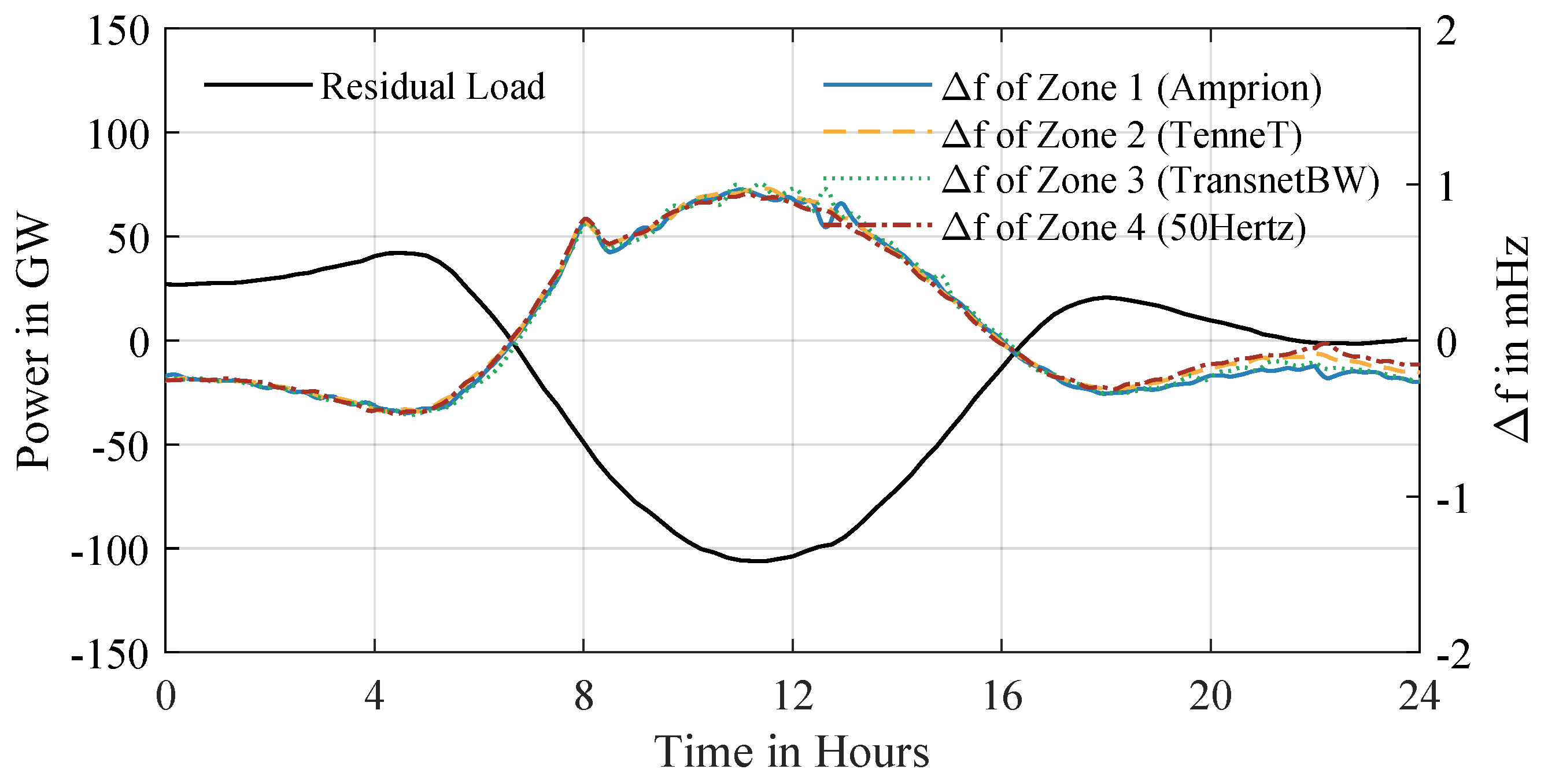
Transitioning from isolated zones to a coupled system with inter-zonal power transfer capability, an April case study (Figure 11) illustrates dynamics under high renewable surplus (average residual load: −24.1 GW vs. annual −20.4 GW), where cumulative residual load and frequency deviations across interconnected zones correlate strongly, exhibiting transient frequency spikes during enforced battery-charging phases that replicate sunny-day deviation patterns. Frequency deviations remain bounded within 1 mHz due to coordinated power transfer adjustments between zones, which promptly counteract imbalances; transfer trajectories adhere to Level 1 MPC setpoints until rising absolute transfer power toward day-end aligns with widening frequency differences. An analysis of non-zero transfer trajectories reveals discrete 900-s gradient jumps, synchronized with Level 1 MPC setpoint updates for Level 2 controllers and driven by forecast inaccuracies, though these perturbations exhibit minimal amplitudes and rapid damping, preserving system-wide frequency stability despite forced battery charging events. The coupled scenario highlights how inter-zonal coordination mitigates deviations even under sustained renewable overgeneration, contrasting with isolated zone responses, while maintaining alignment with MPC-defined transfer and storage schedules.
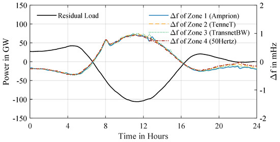
Figure 11.
Simulation results for 21 April 2045: residual load of the four coupled control zones (top) and their frequency deviation from the nominal 50 Hz (bottom). Inter-zonal coupling keeps the zone frequencies nearly identical and within mHz even during transient spikes caused by forced battery charging visible in the residual-load traces.
Further accuracy can be gained by refining both the inputs and the model structure. Updated generation and demand profiles—or tighter dynamic limits—can be substituted without altering the control logic. Because the present formulation relies on a linearized plant, its fidelity is bounded; selected nonlinear effects could be re-introduced as predictable disturbance channels or through unit aggregators. Aggregators condense the behavior of many similar assets (e.g., electric vehicles), capturing individual constraints while keeping the MPC tractable. The same principle can extend to electrolyzers and fuel-cell stacks—where start-up heating or cycling limits matter—yielding a richer yet still manageable representation and, ultimately, more robust results.
3.3. Frequency Behavior
The stability of an energy system depends on its response to unexpected disturbances. Given the two HiMPC layers and the zero-exchange stress case, this section illustrates how independent and interconnected zones within the framework behave under such conditions.
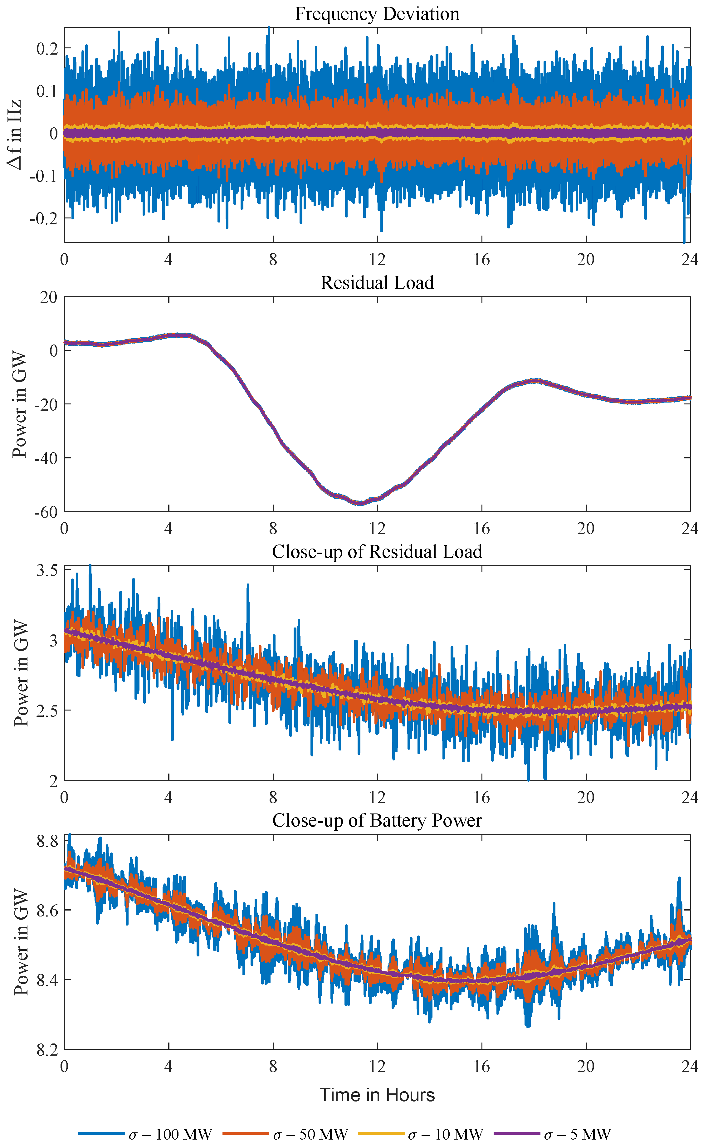
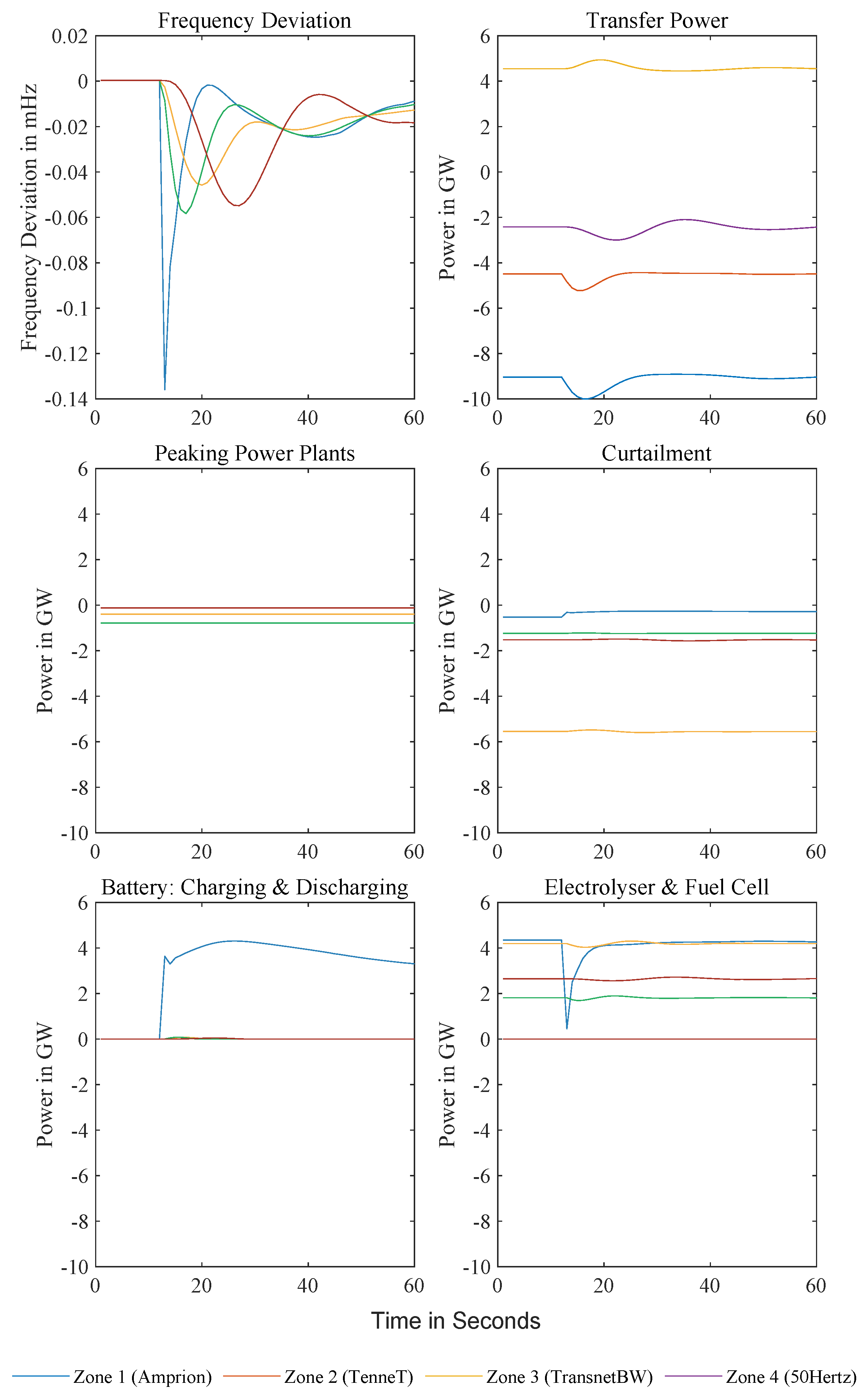
Disturbances are simulated by applying noise with standard deviations of 5–100 MW to real-time wind, photovoltaic generation, and load profiles in isolated Zone 2 (selected for its high conventional power plant’s capacity), while forecasts remain unperturbed due to pre-filtering. Figure 12 shows frequency deviations exceeding the 0.2 Hz threshold at = 100 MW with deviations scaling proportionally to noise intensity. A detailed hourly snapshot reveals unpredictable power jumps up to 1 GW. Because the Level 2 MPC has no prior knowledge of this noise, it compensates only after observing the resulting frequency deviations each second, largely by mobilizing battery capacity; the residual mismatch is therefore mirrored in the frequency trajectory.
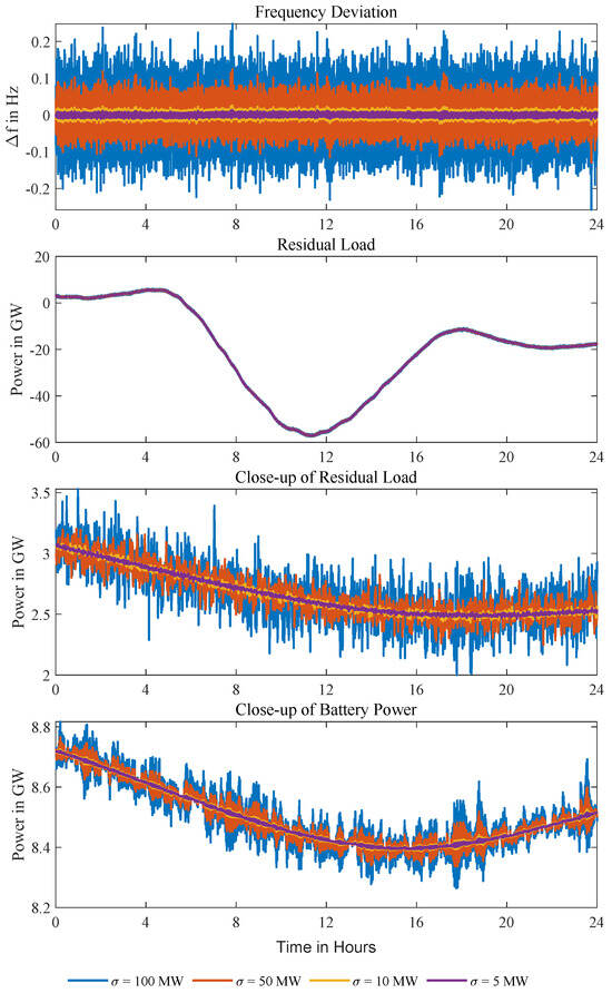
Figure 12.
Frequency deviations in isolated Zone 2 (highest renewable capacity) under load and generation noise with varying standard deviations on an April day. At = 100 MW, deviations exceed the 0.2 Hz threshold, demonstrating the Level 2 MPC’s reliance on battery response for rapid balancing. Unpredictable noise induces instantaneous power jumps up to 1 GW, highlighting challenges in stabilizing purely reactive systems without disturbance forecasts.
To illustrate how coupling mitigates these effects, noise (standard deviations scaled to zone-specific parameters: nominal power , inertia H, and damping ) is applied uniformly across all zones, yielding MW (Zone 1), MW (Zone 3), and MW (Zone 4), which are normalized to Zone 2’s 10 MW baseline. This harmonization limits frequency deviations to ±20 mHz, and zone-averaged frequencies remain tightly aligned, providing direct evidence that inter-zonal coupling stabilizes the system and allows continued adherence to transfer setpoints despite disturbances. While these artificial variations probe stability limits, practical noise scenarios would include additional factors as detailed in [52].
A follow-up test on April 21 in Zone 2 (retaining the model’s highest conventional capacity) evaluates sudden generation loss impacts by simulating a 1 GW load spike at 12:00:01. The Level 2 MPC responds immediately via battery reserves without Level 1 guidance, while the Level 1 MPC detects the event after 15 min, updating long-term strategies using Level 2’s revised operating conditions. This sequence mirrors real-world contingencies: rapid containment by the fast layer followed by strategic recalibration at the slower layer.
Prior to evaluating coupled zone interactions, preliminary simulations characterize the impact of abrupt load variations on frequency deviations in isolated configurations. A 500 MW jump is balanced within 10 s, with a maximum frequency deviation of 37 mHz, while a 1 GW jump briefly exceeds the 0.2 Hz limit by 1 mHz for one second and requires 38 s to stabilize. The model assumes peak-load power plants ramp up at 6.7% per minute (15 min to full capacity), reflecting typical plant characteristics and the overlay system’s time step. Tests with higher ramp rates (15%/min and 200%/min, equivalent to a 30-s ramp-up) demonstrate that increased flexibility reduces balancing times and frequency deviations. During the load jump, batteries respond instantaneously, while peak-load plants ramp up at their maximum rate; over time, battery output is gradually replaced by peak-load generation, which initially operates in the negative region due to concurrent pumped storage charging. The coupled system’s response to a 1 GW load jump in Zone 1 (replicating the isolated case timing and magnitude) demonstrates frequency deviation damping through inter-zonal coupling, reducing Zone 1’s maximum deviation to 88 mHz—below the 0.2 Hz limit—while Zone 4 experiences the highest deviation at 115 mHz. Oscillatory frequency behavior persists for 40 s post-jump, with stabilization delayed compared to isolated cases, reflecting prolonged power transfer oscillations. Adjustments rely on peaking power plants, battery reserves, and renewable curtailment; Zone 1 resolves the jump primarily via full battery deployment and peaking plant ramping, while other zones modulate batteries and curtail renewables without activating peaking plants; the latter are constrained by unchanged setpoints and insensitivity to cross-zone frequency influences. Discrepancies between scheduled and actual power transfers emerge post-jump, necessitating communication or revised transfer computation for alignment; sustained jumps incorporated into Level 1 predictions trigger transfer adjustments. Maximum sustainable load jumps depend on zone-specific parameters and states: isolated Zone 1 exceeds limits by 1 mHz at 1 GW (41.6 GW stabilizing power , full battery reserves), while coupled simulations fail at 1.4 GW with Zone 4 frequency dropping 0.18 Hz at 1.3 GW. Minor battery charging and renewable curtailment inaccuracies, attributable to optimization tolerances, could be mitigated through refined iteration strategies.
The future system model, featuring significantly higher battery capacities (dependent on vehicle-to-grid fleet availability), demonstrates enhanced resilience to extreme load jumps. In isolated Zone 1 simulations, the system balances transient spikes up to 60 GW—and theoretically higher magnitudes short term—primarily via rapid battery response, flexible load adjustments, and the reactivation of curtailed renewables. Frequency oscillations, induced by the 1-s sampling rate and discretization effects in the state-space model, arise from high battery power change rates integrated into frequency calculations. The MPC initially counteracts load jumps through modulation, converging to steady-state power adjustments within 100 s; this strategy temporarily doubles the jump’s amplitude at inception to minimize frequency deviations. However, coupled system simulations reveal amplified oscillations, with Zone 3 deviations reaching 0.19 Hz under a 2.5 GW load jump in Zone 1, underscoring suboptimal MPC tuning for realistic frequency stabilization.
To mitigate oscillations without altering sampling rates, two modifications are implemented: (1) an increased weighting of penalties in the Level 2 MPC, prioritizing direct power balancing over transient rate adjustments, and (2) conditional reference trajectories for inter-zonal power transfers, transitioning to ramp-like setpoints if cumulative deviations exceed 100 MW. Post-adjustments, isolated Zone 1 frequency deviations peak at 0.15 Hz with minimal oscillation, stabilizing within 4 min via phased battery discharge and flexible load coordination. Coupled systems (see Figure 13) exhibit further damping, limiting deviations to 0.14 Hz and enabling transient load jump absorption up to 10 GW. The future system’s capacity hinges on high battery reserves (e.g., 41.6 GW stabilizing power ) and fast response times, though practical limits persist: Zone 1’s peak conventional load (34 GW) and gas plant capacities (30–350 MW/plant) suggest even a 2 GW plant loss remains manageable. Critical vulnerabilities include a low battery state of charge during jumps and reliance on vehicle-to-grid availability, necessitating ancillary safeguards like grid-booster storage or state of charge prioritization in MPC weightings.
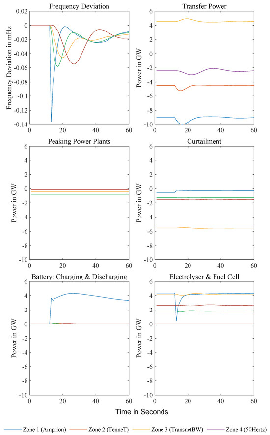
Figure 13.
Frequency deviations in coupled zones following a 10 GW load jump. The figure illustrates the resulting transfer power flows along with the generation and storage system outputs employed for system balancing. Controller performance is enhanced via an adjustment of the weighting matrix ().
The disturbance tests reveal several directions for strengthening the HiMPC framework. Although a simple moving-average filter can smooth the high- noise injected into the simulations, the largest excursions persist because the disturbance propagates simultaneously into frequency and power-transfer setpoints; durable mitigation therefore requires enhancements at the control layer rather than signal post-processing alone. At the opposite end of the spectrum, the 10 GW load-jump experiment—an intentionally severe stress case—demonstrates that a dedicated, fast-acting Grid-Booster battery block can absorb extreme events without resorting to load shedding or renewable curtailment. Such jumps are increasingly unlikely in an ever more decentralized grid, yet the exercise underlines the value of maintaining a strategic reserve of highly responsive storage.
From an implementation perspective, the present Level 2 controller employs a one-second sampling interval and a single-step horizon to keep solve times tractable; finer sampling or longer horizons would sharpen disturbance rejection, particularly for unforecasted jumps, but will require faster optimization routines or parallel hardware. The empirical retuning of the penalties and the introduction of ramp-like transfer references effectively damped the oscillations observed in the 2045 scenario, but a systematic weight-selection methodology—based on closed-loop performance metrics—would generalize tuning across a wider range of operating conditions. Finally, representing assets through linearized models is expedient yet restrictive; future work will introduce aggregator-based nonlinear models for electrolyzers, fuel-cell stacks, and electric-vehicle fleets, capturing start-up heating cycles, temperature dynamics, and other device-specific constraints while keeping the optimization problem manageable. Together, these refinements promise to enhance the realism, resilience, and policy relevance of the proposed HiMPC framework.
4. Conclusions
This paper introduces a reusable two-layer Hierarchical Model Predictive Control (HiMPC) framework that links 15-min day-ahead scheduling to 1-s real-time frequency control across Germany’s four transmission zones. Each zone solves its own MPC problems locally, while a lightweight coordination layer enforces inter-zonal transfer limits, routing power to the zones with the greatest immediate need. The framework is instantiated with data from German TSOs and the Netzentwicklungsplan (NEP) 2045 baseline; then, it is exercised in a stringent zero-exchange (autarky) scenario in which Germany must meet all demand without cross-border assistance. In year-long simulations, the hierarchy keeps system frequency within a few millihertz of the 50 Hz target under sharp ramps, prolonged renewable lulls, and stochastic disturbances. Level 1 pre-positions flexibility—charging batteries, curtailing electrolyzers, scheduling hydrogen-fueled turbines—while Level 2 issues second-scale setpoint corrections that deploy fast storage and shift sector-coupled loads. This separation of time scales minimizes battery cycling, preserves scarce fuel, and maintains adequate reserves throughout the year-long simulation.
Reliable planning for high-renewables grids demands simulation tools that couple multi-hour scheduling trade-offs with sub-second frequency dynamics. Conventional adequacy studies or single-layer controls abstract away this interaction, risking either optimistic or overly conservative infrastructure choices. By embedding an advanced hierarchical MPC in an integrated framework, we can evaluate storage sizing, sector-coupled demand shifts, and transfer-capacity upgrades with the temporal fidelity needed for policy-relevant assessments. HiMPC fills this gap by solving a 15-min horizon economic dispatch in each zone (with network-constrained transfers) and embedding those setpoints in a 1-s MPC that accounts for frequency dynamics, storage states, and sector-coupled flexibility. Assets are represented through aggregators, so additional batteries, electrolyzers, or demand–response pools can be appended without redesign.
Under the zero-exchange stress case, the hierarchy holds frequency deviations below ±2 mHz for 99.9% of the year and below ±10 mHz during the worst multi-day renewable drought. Batteries absorb sub-second transients; electrolyzers, heat pumps, and vehicle-to-grid technologies shift hundreds of gigawatt-hours of demand; hydrogen turbines cover the longest deficits while operating only 1800–1900 full-load hours a year. Inter-zonal transfers further damp frequency spread, proving that decentralized control can deliver system-wide coherence without a single central optimizer. These outcomes demonstrate the framework’s suitability for capacity-sizing and adequacy-planning studies, making it suitable for policy-relevant scenario assessments of high-renewables grids.
The modular, aggregator-based design means planners can embed new asset classes, explore alternative market rules, or re-parameterize cost functions with minimal code changes. Because the same hierarchy governs slow scheduling and fast dynamics, policy scenarios (e.g., hydrogen build-out levels, battery incentives, transfer-capacity upgrades) can be tested end-to-end without inconsistencies between operational and investment time scales. Although the hierarchy captures the key time-scale interactions, several simplifying assumptions remain. First, each control zone is treated as a copper-plate node, so intra-zonal network constraints and resistive losses are ignored; introducing a linearized or full AC layer would sharpen locational results but at a much higher computational cost. Second, asset behavior is represented through aggregators that abstract technical details such as electrolyzer start-up dynamics or vehicle-to-grid availability; richer sub-models could alter the estimated flexibility margins. Third, the simulations rely on a single representative weather year and deterministic forecasts; multi-year probabilistic ensembles would be required for a full risk assessment. These caveats outline clear pathways for future refinement rather than limiting the current framework’s value as a planning tool.
By delivering an open, scalable HiMPC blueprint and demonstrating its performance under an autarky challenge, the work provides both a concrete template for future control implementations and a benchmark dataset against which alternative scheduling-and-control schemes can be compared. Future extensions will integrate nonlinear network models, adaptive forecast updating, and formal robustness certificates; evaluate market-coordinated variants of the hierarchy; and apply the framework to other regional grids to test its portability and scalability.
Author Contributions
Conceptualization, A.B., J.B. and F.K.; Methodology, A.B., J.B. and F.K.; Software, A.B., J.B. and F.K.; Validation, A.B. and J.B.; Formal analysis, A.B. and J.B.; Investigation, A.B. and J.B.; Resources, A.B. and J.B.; Data curation, A.B. and J.B.; Writing—original draft, A.B. and J.B.; Writing—review & editing, A.B. and F.K.; Visualization, A.B. and J.B.; Supervision, F.K.; Project administration, F.K.; Funding acquisition, F.K. All authors have read and agreed to the published version of the manuscript.
Funding
This research was funded by the Carl Zeiss Foundation (P2022-01-018).
Data Availability Statement
The original contributions presented in this study are included in the article. Further inquiries can be directed to the corresponding author.
Conflicts of Interest
The authors declare no conflicts of interest.
References
- Mlilo, N.; Brown, J.; Ahfock, T. Impact of intermittent renewable energy generation penetration on the power system networks—A review. Technol. Econ. Smart Grids Sustain. Energy 2021, 6, 25. [Google Scholar] [CrossRef]
- Yang, C.; Sun, W.; Han, D.; Yin, X. Research on power system flexibility considering uncertainties. Front. Energy Res. 2022, 10, 967220. [Google Scholar] [CrossRef]
- Khan, H.A.; Zuhaib, M.; Rihan, M. A review on voltage and frequency contingencies mitigation technologies in a grid with renewable energy integration. J. Inst. Eng. (India) Ser. B 2022, 103, 2195–2205. [Google Scholar] [CrossRef]
- International Renewable Energy Agency. Renewable Energy Statistics. 2025. Available online: https://www.iea.org/reports/global-energy-review-2025 (accessed on 28 July 2025).
- Kundur, P. Power System Stability and Control; CRC Press: New York, NY, USA, 2007; Volume 10, pp. 1–7. [Google Scholar]
- Barth, A.; González, D.; Gonzalez, J.L.; Hanzlík, V.; Pinheiro, G.; Tai, H.; Weiss, A. How Grid Operators Can Integrate the Coming Wave of Renewable Energy; McKinsey & Company: Chicago, IL, USA, 2024. [Google Scholar]
- Shahzad, S.; Jasińska, E. Renewable revolution: A review of strategic flexibility in future power systems. Sustainability 2024, 16, 5454. [Google Scholar] [CrossRef]
- Elsisi, M.; Soliman, M.; Aboelela, M.A.S.; Mansour, W. Model predictive control of plug-in hybrid electric vehicles for frequency regulation in a smart grid. IET Gener. Transm. Distrib. 2017, 11, 3974–3983. [Google Scholar] [CrossRef]
- Yang, L.; Liu, T.; Hill, D.J. Distributed MPC-based frequency control for multi-area power systems with energy storage. Electr. Power Syst. Res. 2021, 190, 106642. [Google Scholar] [CrossRef]
- Ali, A.; Khan, B.; Mehmood, C.A.; Ullah, Z.; Ali, S.M.; Ullah, R. Decentralized MPC based frequency control for smart grid. In Proceedings of the 2017 International Conference on Energy Conservation and Efficiency (ICECE), Lahore, Pakistan, 22–23 November 2017; IEEE: Piscataway, NJ, USA, 2017; pp. 1–6. [Google Scholar]
- Pandey, S.K.; Mohanty, S.R.; Kishor, N. A literature survey on load–frequency control for conventional and distribution generation power systems. Renew. Sustain. Energy Rev. 2013, 25, 318–334. [Google Scholar] [CrossRef]
- Jiang, H.; Lin, J.; Song, Y.; Hill, D.J. MPC-based frequency control with demand-side participation: A case study in an isolated wind-aluminum power system. IEEE Trans. Power Syst. 2014, 30, 3327–3337. [Google Scholar] [CrossRef]
- Ersdal, A.M.; Imsland, L.; Uhlen, K. Model predictive load-frequency control. IEEE Trans. Power Syst. 2016, 31, 777–785. [Google Scholar] [CrossRef]
- Sultana, W.R.; Sahoo, S.K.; Sukchai, S.; Yamuna, S.; Venkatesh, D. A review on state of art development of model predictive control for renewable energy applications. Renew. Sustain. Energy Rev. 2017, 76, 391–406. [Google Scholar] [CrossRef]
- Shi, Y.; Tuan, H.D.; Savkin, A.V.; Duong, T.Q.; Poor, H.V. Model predictive control for smart grids with multiple electric-vehicle charging stations. IEEE Trans. Smart Grid 2018, 10, 2127–2136. [Google Scholar] [CrossRef]
- Vlahakis, E.E.; Dritsas, L.D.; Halikias, G.D. Distributed Model Predictive Load Frequency Control of multi-area Power Grid: A Decoupling Approach. IFAC-PapersOnLine 2019, 52, 205–210. [Google Scholar] [CrossRef]
- Ferro, G.; Robba, M.; Sacile, R. A Fully Distributed Robust MPC Approach for Frequency and Voltage Regulation in Smart Grids With Active and Reactive Power Constraints. IEEE Trans. Syst. Man Cybern. Syst. 2024, 54, 6657–6669. [Google Scholar] [CrossRef]
- Wang, R.; Wang, M.; Wang, K.; Wang, X. Optimization of frequency dynamic characteristics in microgrids: An improved MPC-VSG control. Int. J. Electr. Power Energy Syst. 2024, 156, 109783. [Google Scholar] [CrossRef]
- Liu, X.; Wang, C.; Kong, X.; Zhang, Y.; Wang, W.; Lee, K.Y. Tube-Based Distributed MPC for Load Frequency Control of Power System With High Wind Power Penetration. IEEE Trans. Power Syst. 2024, 39, 3118–3129. [Google Scholar] [CrossRef]
- An, Z.; Liu, X.; Xiao, G.; Song, G.; Wang, P. Tube-based MPC strategy for load frequency control of multi-area interconnected power system with HESS. J. Energy Storage 2024, 99, 113340. [Google Scholar] [CrossRef]
- Scattolini, R. Architecture of Distributed and Hierarchical Model Predictive Control—A Review. J. Process Control 2009, 19, 723–731. [Google Scholar] [CrossRef]
- Kong, X.; Liu, X.; Ma, L.; Lee, K.Y. Hierarchical Distributed Model Predictive Control of Standalone Wind/Solar/Battery Power System. IEEE Trans. Syst. Man Cybern. Syst. 2019, 49, 1570–1581. [Google Scholar] [CrossRef]
- Babayomi, O.; Zhang, Z.; Dragicevic, T.; Hu, J.; Rodriguez, J. Smart grid evolution: Predictive control of distributed energy resources—A review. Int. J. Electr. Power Energy Syst. 2023, 147, 108812. [Google Scholar] [CrossRef]
- Kennel, F.; Gorges, D.; Liu, S. Energy management for smart grids with electric vehicles based on hierarchical MPC. IEEE Trans. Industr. Inform. 2013, 9, 1528–1537. [Google Scholar] [CrossRef]
- Darudi, A.; Savelsberg, J.; Schlecht, I. Thrive in Sunshine, Brace for Thunder: Least-Cost Robust Power System Investments Under Political Shocks; Technical Report; Leibniz Information Centre for Economics: Kiel, Germany; Hamburg, Germany, 2024. [Google Scholar]
- Ahumada-Paras, M.; Mastrandrea, M.; Wara, M. Grid Regionalization in the West: Reliability Benefits from Increased Cooperation in Electricity Markets and Operations; Technical Report; Stanford Woods Institute for the Environment: Stanford, CA, USA, 2024. [Google Scholar]
- Med-TSO. Seasonal Adequacy Assessment: Summer Outlook 2024; Technical report; Mediterranean Transmission System Operators: Rome, Italy, 2024. [Google Scholar]
- Liedekerke, A.V.; Gjorgiev, B.; Savelsberg, J.; Wen, X.; Dujardin, J.; Darudi, A.; Sasse, J.P.; Trutnevyte, E.; Lehning, M.; Sansavini, G. Policy-relevance of a model inter-comparison: Switzerland in the European energy transition. Appl. Energy 2025, 391, 125906. [Google Scholar] [CrossRef]
- Sulzer, M.; Mavromatidis, G.; Nuñez-Jimenez, A.; Wetter, M. The Energy Supply Security Pyramid: A Quantitative Framework for Planning and Policy Making. iScience 2025, 28, 112407. [Google Scholar] [CrossRef]
- Zachmann, G.; Batlle, C.; Beaude, F.; Maurer, C.; Morawiecka, M.; Roques, F. Unity in Power, Power in Unity: Why the EU Needs More Integrated Electricity Markets; Technical report, Bruegel Policy Brief 2024/03; Bruegel: Saint-Josse-ten-Noode, Brussels, 2024. [Google Scholar]
- Federal Network Agency (Bundesnetzagentur or BNetzA). Netzentwicklungsplan Strom 2037 mit Ausblick 2045, Zweiter Entwurf der Übertragungsnetzbetreiber; Technical report; Bundesnetzagentur für Elektrizität, Gas, Telekommunikation, Post und Eisenbahnen: Bonn, Germany, 2023. [Google Scholar]
- Morren, J.; De Haan, S.W.; Kling, W.L.; Ferreira, J. Wind turbines emulating inertia and supporting primary frequency control. IEEE Trans. Power Syst. 2006, 21, 433–434. [Google Scholar] [CrossRef]
- Fernández-Guillamón, A.; Gómez-Lázaro, E.; Muljadi, E.; Molina-García, Á. Power systems with high renewable energy sources: A review of inertia and frequency control strategies over time. Renew. Sustain. Energy Rev. 2019, 115, 109369. [Google Scholar] [CrossRef]
- Wu, Z.; Gao, W.; Gao, T.; Yan, W.; Zhang, H.; Yan, S.; Wang, X. State-of-the-art review on frequency response of wind power plants in power systems. J. Mod. Power Syst. Clean Energy 2018, 6, 1–16. [Google Scholar] [CrossRef]
- Zertek, A.; Verbic, G.; Pantos, M. Participation of DFIG wind turbines in frequency control ancillary service by optimized rotational kinetic energy. In Proceedings of the 2010 7th International Conference on the European Energy Market, Madrid, Spain, 23–25 June 2010; IEEE: Piscataway, NJ, USA, 2010; pp. 1–6. [Google Scholar]
- Andersson, G. Dynamics and Control of Electric Power Systems; Lecture Script; ETH–Power Systems Laboratory: Zurich, Switzerland, 2010. [Google Scholar]
- Domahidi, A.; Zgraggen, A.U.; Zeilinger, M.N.; Morari, M.; Jones, C.N. Efficient interior point methods for multistage problems arising in receding horizon control. In Proceedings of the 2012 IEEE 51st IEEE Conference on Decision and Control (CDC), Maui, HI, USA, 10–13 December 2012; pp. 668–674. [Google Scholar] [CrossRef]
- Aswani, A.; Bouffard, P.; Zhang, X.; Tomlin, C. Practical comparison of optimization algorithms for learning-based MPC with linear models. arXiv 2014, arXiv:1404.2843. [Google Scholar] [CrossRef]
- Rauls, E.; Hehemann, M.; Keller, R.; Scheepers, F.; Müller, M.; Stolten, D. Favorable Start-Up behavior of polymer electrolyte membrane water electrolyzers. Appl. Energy 2023, 330, 120350. [Google Scholar] [CrossRef]
- De Jonghe, C.; Delarue, E.; Belmans, R.; D’haeseleer, W. Determining optimal electricity technology mix with high level of wind power penetration. Appl. Energy 2011, 88, 2231–2238. [Google Scholar] [CrossRef]
- Hentschel, J.; Babic, U.; Hartmut, S. A parametric approach for the valuation of power plant flexibility options. Energy Rep. 2016, 2, 40–47. [Google Scholar] [CrossRef]
- Nant de Drance SA. The Power Plant—Key Figures 2025. Available online: https://www.nant-de-drance.ch/en/the-power-plant (accessed on 21 September 2025).
- Tan, K.M.; Ramachandaramurthy, V.K.; Yong, J.Y. Bidirectional battery charger for electric vehicle. In Proceedings of the 2014 IEEE Innovative Smart Grid Technologies-Asia (ISGT ASIA), Kuala Lumpur, Malaysia, 20–23 May 2014; IEEE: Piscataway, NJ, USA, 2014; pp. 406–411. [Google Scholar]
- Hodges, A.; Hoang, A.L.; Tsekouras, G.; Wagner, K.; Lee, C.Y.; Swiegers, G.F.; Wallace, G.G. A high-performance capillary-fed electrolysis cell promises more cost-competitive renewable hydrogen. Nat. Commun. 2022, 13, 1304. [Google Scholar] [CrossRef]
- Sazali, N.; Wan Salleh, W.N.; Jamaludin, A.S.; Mhd Razali, M.N. New perspectives on fuel cell technology: A brief review. Membranes 2020, 10, 99. [Google Scholar] [CrossRef]
- International Energy Agency. Technology: Pumped Hydroelectric Energy Storage (Fact Sheet). 2024. Available online: https://iea-es.org/wp-content/uploads/public/FactSheet_Mechanical_Pumped_Hydroelectric.pdf (accessed on 21 September 2025).
- Follmer, R. Mobilität in Deutschland: Ergebnisbericht; infas—Institut für Angewandte Sozialwissenschaft GmbH: Bonn, Germany, 2004; p. 187. [Google Scholar]
- Boecker, J.; Bösing, M.; Bredehorn, M.; Canders, W.R.; Cebulski, B.; Doetsch, P.; Doncker, R.D.; Kashani, O.F.; Friedrich, B. VDE-Studie Elektrofahrzeuge; VDE e.V.: Offenbach, Germany, 2010. [Google Scholar]
- Eichman, J.; Harrison, K.; Peters, M. Novel Electrolyzer Applications: Providing More Than Just Hydrogen; Technical report; Office of Scientific and Technical Information (OSTI): Oak Ridge, TN, USA, 2014. [Google Scholar] [CrossRef]
- Eichhorn Colombo, K.W.; Kharton, V.V. Start-Up of a Solid Oxide Fuel Cell System with a View to Materials Science-Related Aspects, Control and Thermo-Mechanical Stresses. Crystals 2021, 11, 732. [Google Scholar] [CrossRef]
- Bundesverband der Energie- und Wasserwirtschaft e. V. (BDEW). Standardlastprofile Strom—Grundlagen & Anwendung; Bundesverband der Energie- und Wasserwirtschaft e. V. (BDEW): Berlin, Germany, 2025. [Google Scholar]
- Michigami, T.; Oishi, T. Construction of dynamic fluctuation load model and simulation with AFC-control of BTB interconnection. IEEJ Trans. Power Energy 2000, 120, 954–961. [Google Scholar] [CrossRef] [PubMed][Green Version]
Disclaimer/Publisher’s Note: The statements, opinions and data contained in all publications are solely those of the individual author(s) and contributor(s) and not of MDPI and/or the editor(s). MDPI and/or the editor(s) disclaim responsibility for any injury to people or property resulting from any ideas, methods, instructions or products referred to in the content. |
© 2025 by the authors. Licensee MDPI, Basel, Switzerland. This article is an open access article distributed under the terms and conditions of the Creative Commons Attribution (CC BY) license (https://creativecommons.org/licenses/by/4.0/).


