Abstract
This paper proposes a household energy management system for all-electric households, focusing on the interplay between cost savings and occupant comfort through an implicit demand response programme. A sequential multi-objective optimisation model is developed based on the lexicographic approach, allowing for the effective prioritisation of objectives. The model optimally schedules a diverse range of electricity demands using real-world data from a Norwegian pilot household to evaluate its unique flexibility potential, while remaining adaptable for other regions. This includes integrating thermal and non-thermal demands with electric mobility via vehicle-to-home enabled electric vehicle charger. This approach achieves significant cost savings on energy bills and enhances user comfort across aggregated comfort indicators. Multiple scenarios are designed to evaluate the performance of the proposed demand response under diverse pricing mechanisms. Results indicate that transitioning from variable pricing to fixed pricing can lead to lower average electricity costs and higher average user comfort. The analysis reveals that prioritising occupant comfort can substantially increase electricity demand, resulting in a nearly fourfold rise in average annual expenses, while also leading to a decrease in self-consumption and self-sufficiency. Additionally, the study illustrates how grid tariff adjustments can benefit households and support the development of local renewable energy.
1. Introduction
The global push for renewable energy resources emphasises the promotion of household solar photovoltaic (PV) installations. The advancement of solar energy is influenced by the unique characteristics of each region, including land availability. In Norway, a strong reliance on hydropower and distinct geographical features have led to a slower pace of adoption of other renewable energy sources [1] compared to leading European nations like Denmark [2]. In 2024, Norway added approximately 149 MW of new solar PV capacity, raising its total installed PV capacity to over 753.67 MW, a modest figure globally but significant given Norway’s high latitude and low solar irradiation in winter [3]. Electricity demand is rising in both the industrial and residential sectors. However, the further development of hydropower is constrained by environmental protection considerations [2]. This is expected to result in a national electricity consumption increase of 24 TWh, exceeding the planned growth of 6 TWh in power production until 2027 [4]. This underscores the importance of contributions from distributed energy production, particularly PV installations in the building sector, as they can be placed on existing rooftops. The Norwegian residential sector accounts for 22% of the total energy consumption [5], where approximately 70% of household energy is dedicated to space heating and domestic hot water [6]. Heat pumps (HPs) function by extracting heat from the outdoor air, even at low ambient temperatures, and converting it for use within buildings during the winter months. As the European leader in HP per capita, Norway’s residential sector offers considerable opportunities for nationwide energy savings and flexibility [7]. This potential is anticipated to offer flexibility of around 1000 MW from water heating and 1200–1700 MW from space heating [8]. In line with the EU directive on the energy performance of buildings [9], the nearly-Zero-Energy Building (nZEB) concept is gaining traction in Norway, with an emphasis on utilising PV energy production for on-site or nearby energy supply [10]. Furthermore, Norway has established itself as a global frontrunner in Electric Vehicle (EV) adoption, notably diverging from trends in the wider European market [11]. As of April 2024, EVs make up 90% of all new car sales in the country [12], leading to a total of over 850,000 EVs in service [13]. This impressive adoption rate has led to more EVs than gasoline cars on Norway’s roads [14]. With the integration of vehicle-to-grid (V2G) and vehicle-to-home (V2H) through smart bidirectional chargers [15], it is technologically possible to leverage the flexibility of EVs as “batteries on wheels” [16]. This allows for electricity flow from the vehicle to either the home or the main grid, helping to manage electricity price fluctuations and absorb excess PV energy production [17]. Hvidsten et al. demonstrated that in a future Norwegian net-zero electricity system, just 50% participation of EVs in V2G schemes could eliminate the need for stationary battery storage, leading to system cost reductions of about 4% and up to 15% under full participation [18]. However, the real-world implementation of V2H technology faces several challenges. Social acceptance is affected by concerns regarding battery degradation, range anxiety related to travel distance, and the potential loss of control, comfort, and convenience over charging or discharging [19]. The discharge capacity depends on the vehicle’s battery capacity, the time remained plugged in, and various operational factors impacting the total energy available [20].
To effectively manage household energy, a residential energy scheduler can be employed within a household energy management system (HEMS) to identify optimal switching decisions for electricity demands. This approach integrates a battery-free PV setup and EV, all tailored to the customer’s objectives and preferences [21]. Demand response (DR) programmes are key strategies for managing demand-side resources through prices or incentives. Price-based DR (implicit DR) allows consumers to adjust energy usage in response to time-varying electricity prices, optimising for cost or grid stability, while incentive-based DR (explicit DR) enables consumers to offer flexibility in dedicated markets via contracts or aggregators [22]. In terms of implementation, price-based DR offers several advantages over incentive-based by facilitating efficient response to price changes [23], such as simplicity and accessibility, reduced implementation costs, and increased consumer autonomy and engagement [24]. Hofmann and Lindberg demonstrated that integrating dynamic hourly pricing with smart HEMS, incorporating PV and EV, can enhance household energy flexibility by up to 20%. This integration with automated DR enables peak load reductions of up to 15.7% during peak hours [25]. Similarly, Backe et al. showed that activating energy demand flexibility through pre-defined strategies like flattening demand or aligning with time-of-use tariffs in the highly electrified building stock of Norway can reduce peak load by 10–12% and lower system costs by 80–90% by 2040 [26].
The primary motivator for the widespread adoption of DR programmes is the electricity cost savings achieved through the effective and efficient HEMS [27]. Additionally, it is essential to consider the trade-off between cost and comfort in DR programmes, particularly in all-electric Norwegian households that are concerned about how energy flexibility affects their comfort and convenience [28]. Although ensuring acceptable levels of thermal comfort is fundamental for user convenience and satisfaction, not all the DR control algorithms are developed to minimise costs while keeping comfort within acceptable limits [29]. Wang et al. proposed a multi-objective residential load dispatch strategy [30]. Using Time of Use (ToU) pricing, which charges different rates for electricity based on the time of day, and economic incentives, the model evaluated comfort, response fatigue, and plan satisfaction. They utilised an aggregator-level model for user task allocation rather than a user-driven model. Simulations showed enhanced user satisfaction and maximised revenues [30]. Yao et al. developed an optimal load scheduling scheme for smart homes based on weighted optimisation, emphasising user preference and convenience [31]. The scheduler minimised costs, maximised convenience, and enhanced comfort in HEMS [31]. However, the proposed model focused exclusively on appliances and did not address thermal and electric mobility (e-mobility) demands. Despite numerous efforts to quantitatively evaluate cost and comfort in DR optimisation, a gap persists in creating comprehensive models that incorporate a diverse range of electricity demands and analyse the role of tariff schemes. The analysis of existing literature underscores the need for a comprehensive multi-objective DR optimisation, enabling an effective and integrated balance of competing priorities such as cost savings and user comfort, in managing various household electricity demands.
The multi-objective nature of DR optimisation necessitates the use of various mathematical methods to handle the complexity of balancing different objectives. In terms of prioritisation, the lexicographic method serves as an effective approach for managing multi-objective optimisation, enabling the achievement of optimal solutions [32]. This method first optimises the highest-priority objective, followed by the optimisation of lower-priority objectives, ensuring that the values of the higher-priority objectives are preserved. There are few studies that have employed the lexicographic method for HEMS. Tostado-Véliz et al. proposed a lexicographic ordering of objectives, designating household electricity cost as the primary objective and comfort as the secondary objective [33]. In another study, Tostado-Véliz et al. developed an approach that achieved a balanced solution between electricity costs and thermal comfort, resulting in a scheduling plan that satisfactorily optimised all objectives [34]. In a follow-up research, Tostado-Véliz et al. highlighted that the primary objective in household DR is to minimise electricity costs, while also considering secondary objectives such as maximising thermal comfort, minimising waiting times for interruptible and non-interruptible appliances, and reducing battery energy storage system degradation. These objectives worked together to enhance user convenience and promote efficient energy consumption [35]. Tostado-Véliz et al. also introduced a methodology for HEMS in nZEBs, utilising lexicographic optimisation to jointly optimise electricity cost and net consumption [36]. This approach enabled the identification of compromise solutions while addressing uncertainties associated with renewable energy production and EV behaviour [36]. Gheouany et al. employed the lexicographic method to address a HEMS using multi-objective Mixed-Integer Non-Linear Programming (MINLP) [37]. Their model aimed at minimising the electricity bill, peak load, and appliances’ operating waiting time, while maintaining optimality in relation to previously optimised objectives and sensitivity to the order of the objective functions [37]. While integrating various objectives and addressing uncertainties, the various studies cited reveal a gap in the detailed trade-off analysis of these objectives. Additionally, there is a tendency to rely on simulations without real-world testing and to neglect the integration of diverse electricity demand types and thermodynamic details in practical settings. This oversight limits the generalizability of findings across different household contexts. Previous work by the authors [38] developed a residential demand-side management model for a solar-integrated all-electric house across three engagement levels: uninterested, engaged, and proactive prosumers. The single-objective optimisation model, limited to a one-day operational period, hindered the capture of seasonal variations and effectively addressing the cost-comfort trade-off in household DR scheduling. Additionally, it did not account for realistic V2H-enabled EV functionality or the impact of grid tariff structures on household flexibility.
The economic feasibility of DR programmes is directly influenced by regional tariff design, societal implications, and government incentives [39]. These factors significantly shape the development of small-scale renewable energy production, as evidenced by the policies that have stimulated investment in PV installations among Norwegian households in recent years [40]. An investigation into grid tariff schemes for demand-side management in all-electric houses in Norway by Karlsen et al. demonstrated that all tariff structures incentivised load shifting and reduced peak demand [41]. The Tiered Rate (TR) provided the highest savings per kilowatt-hour shifted by setting subscription limits and overused charges that encourage load reduction above certain thresholds. The ToU tariff promoted load shifting by varying energy prices throughout the day, motivating users to shift consumption to lower-cost periods but requiring increased flexibility. Additionally, the Measured Power (MP) tariff reduced annual costs by charging based on peak power demand during a measurement period, incentivising users to lower their highest loads [42]. Similarly, Garnache et al. reported a 15.3% reduction in peak electricity use, primarily through EVs shifting to off-peak times [43]. This was achieved with a ten-fold price increase, as households adjusted their behaviour in response to critical peak pricing (CPP), leading to load shifting and demand reductions during peak hours. Recent studies indicate that dynamic grid tariffs may exacerbate social inequalities, with households possessing greater flexibility and resources benefiting more from DR programmes, while vulnerable groups face heightened costs and discomfort. Winther and Sundet demonstrate that unequal access to flexibility results in disparate outcomes, underscoring the necessity of integrating justice considerations into tariff design [28]. Addressing these disparities through justice-aware DR models can foster a more equitable energy transition, particularly within Nordic contexts characterised by diverse societal needs. The above studies illustrate an open research area for detailed household modelling to understand better and optimise the effects of tariff structures and social perspectives on the potential participants of DR programmes.
This paper presents a comprehensive Household Energy Scheduler (HES) for managing diverse electricity demands by integrating thermal requirements, non-thermal loads, and e-mobility. The goal is to optimise electricity demand scheduling in relation to self-supply from PV energy production. The proposed model incorporates thermodynamic details of the thermal system, specifically focusing on HP’s water tanks and indoor climate, alongside commonly used shiftable and non-shiftable appliances. Furthermore, it integrates the EV charging and discharging capabilities through smart charging V2H technology. To achieve these, a novel sequential multi-objective optimisation approach based on the lexicographic method is developed and employed, allowing prioritisation of either cost saving or comfort as the main objective. This choice is based on household preferences and allows for multi-objective optimisation rather than pre-allocated engagement levels. This study therefore contributes to a deeper understanding of the cost-comfort trade-off in a fully electrified solar-integrated pilot house, leveraging real-world data for a more reliable assessment specifically in cold-climate regions. Furthermore, the model emphasises Norway’s unique flexibility potential in electricity demands for heating and e-mobility, along with different solar PV production patterns, while remaining applicable to other regions with minimal modifications. Analysing both hourly snapshots and prolonged runs reveals the effectiveness of the proposed approach in optimising electricity demand and household transactions with the grid. Additionally, multiple cost-priority and comfort-priority scenarios are defined to evaluate the performance of the proposed implicit DR programme under various grid tariff designs, including variable pricing and fixed pricing. This study also explores how adjustments to the grid tariff model can foster renewable developments and benefit households through innovative mechanisms such as local energy trading.
The remainder of this paper is structured as follows: Section 2 outlines the modelling of the multi-objective optimisation problem for the proposed implicit DR programme. Section 3 showcases the living lab case study conducted on a Norwegian household. Section 4 examines the results obtained from the study from both hourly and prolonged analyses perspectives. Finally, Section 5 provides the conclusions and highlights potential future research directions.
2. Modelling
2.1. Household Electricity Demands
The focus of the modelling practice is on the daily energy management of a fully electric household. The proposed price-based DR programme identifies the optimal strategy for scheduling the household’s electricity demands given the input data. As this study aims to provide an inclusive analysis in a real-world setup, various demands are considered in the presence of PV energy production. These demands include thermal, non-thermal, and e-mobility needs. Thermal demand is divided into space heating and water heating, while non-thermal demands account for shiftable and non-shiftable demands based on their criticality in activation time [44], and e-mobility pertains to home EV charger.
- Thermal demands: The heating requirements of a household encompass both space heating and water heating. An effective solution for meeting both requirements is the Air-Source Electric Heat Pump Water Heater (HPWH), which extracts heat from the outdoor air and transfers it to the water via a heat exchanger, efficiently addressing both heating needs [45]. Thermal performance of a building is significantly influenced by environmental conditions, occupancy patterns, and building materials. The proposed model formulates the building’s heat capacity and heat loss rate by utilising input data in conjunction with information from thermal systems and building thermal specifications [46]. These input data are utilised to optimise a simplified thermal storage model that facilitates energy shifting through the storage of heat in water tanks and interior air [47]. The thermodynamic behaviour of HPWH and the building is represented through various terms in objectives, along with multiple constraints that support effective and scalable HES. The model helps set the indoor temperature and domestic hot water within the user’s preferred range, while also minimising energy costs and maximising comfort. This is accomplished by establishing thermal variables, specifically the temperatures of the sections.
- Non-thermal demand: In a household, these electricity demands consist of various electric appliances that can be categorised into two primary groups: time-shiftable and non-time-shiftable appliances. Non-shiftable appliances, which cannot be deferred, include essential devices such as lighting, stove, refrigerator, television, computer, router, microwave, and coffee machine. In contrast, shiftable appliances can be postponed and comprise appliances like dishwasher, vacuum cleaner, and washing machine. For shiftable demands, users specify a continuous range of acceptable activation times throughout the day, allowing the optimisation model to determine the most efficient scheduling strategy.
- E-mobility demand: This category of all-electric household electricity demands emphasises smart EV charging based on daily driving patterns and the vehicle’s presence at home. The charging needs of an EV can vary significantly depending on daily commuting habits and the amount of time the vehicle remains parked. This category includes scheduling strategies that optimise charging times to take advantage of lower electricity rates and available solar energy. Users can input details about typical EV usage pattern, allowing the optimisation model to establish the most efficient charging schedule that meets commuting energy requirements while aligning with other energy management objectives. Additionally, concepts like V2H represent opportunities for EVs to both consume and supply electricity. However, real-world limitations, such as restrictions set by manufacturers on total discharging energy over vehicle’s lifetime, need to be considered in HES when integrating these technologies.
Similarly to EV batteries and thermal storage, battery storage can contribute significantly to the flexibility of households. However, it was not considered in this Norwegian household model due to a focus on the available flexible resources present in many Norwegian households, including the pilot house examined. In addition, integrating battery storage requires an investment analysis of its economic viability in accordance with regional policies. This study establishes a baseline and proposes directions for future research that could incorporate these technologies.
2.2. Multi-Objective Optimisation Approach
The subsequent section details the development of a multi-objective optimisation approach aimed at identifying optimal scheduling of household electricity demands. In this study, the primary objectives are cost savings and comfort. To effectively balance these competing priorities, a lexicographic method is employed in the modelling approach. This sequential multi-objective optimisation process prioritises objectives, allowing users to evaluate how different priorities based on their energy preferences impact HES and economic efficiency. By defining their first objective, which may prioritise cost saving or comfort [48], users establish a clear hierarchy that guides the optimisation process [49]. For example, if the study consistently prioritises cost-saving as the first objective, the model can identify solutions that minimise expenses related to energy consumption. Once the optimal value of the first objective is achieved and its value stored, and the other variables are reset, the model then optimises the remaining objectives, such as comfort. The process of storing the value of the first objective is followed by resetting and reinitialising the other decision variables in the optimisation model during the transition between layers. The optimisation is solved again, this time considering the next optimisation objective based on the prioritised list of objectives, with an additional constraint. The objective function of the first layer is now added as a constraint with the limit equal to the value of the objective function found in the previous layer. This is essential to guarantee that the first layer of optimisation does not affect the second layer’s optimisation, except through the added constraint. This approach ensures the integrity of the entire sequential optimisation process and promotes a balanced energy management strategy that aligns with users’ values and preferences. The flowchart in Figure 1 illustrates the sequence of steps in this lexicographic multi-objective optimisation process, which are formulated in the next section.
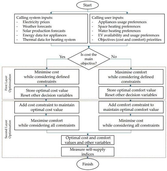
Figure 1.
Flowchart of the sequential multi-objective HES optimisation process.
As discussed in Figure 1, this model addresses two objectives: minimising costs and maximising comfort. These objectives are presented in detail below to facilitate the sequential optimisation process using the lexicographic approach.
2.2.1. Cost Objective
The cost objective function determines a household’s electricity bill and seeks to minimise electricity expenses. This analysis employs the Norwegian electricity billing model, which consists of several components as outlined by Elvia, Norway’s largest distribution network operator [50]. This model utilises variable pricing, where energy costs fluctuate based on demand, supply, and time of day, encouraging consumers to use electricity during off-peak hours when rates are lower. Electricity billing frameworks in Nordic countries incorporate similar components, including fixed, variable, and spot-indexed contracts, plus taxes and grid fees, with varying proportions [51].
- Fixed Term: This term is determined based on the consumption peaks, distinguishing it from the variable hourly rates. This term basically represents the cost associated with average energy consumption during the three highest peak hours within a month, where each peak hour reflects the maximum consumption recorded during a single hour of a day. The monthly add-on for the fixed term (ccap) requires first determining the daily capacity/peak power values, followed by identifying the corresponding step and cost outlined in Table 1. For this model, which analyses a single day, the peak power value for that day is integrated into the fixed term. Subsequently, the monthly billing components are divided by the billing period (m) to approximate the electricity bill for a particular day.
 Table 1. Steps for the fixed term of household electricity bill from the Norwegian DSO [50].
 - Variable Term: This component is determined by electricity (kWh) consumption, and the associated cost fluctuates based on the electricity price at the time of day when it is utilised.
- Public Charges: This term encompasses mandatory payments to the Energy Fund, electricity taxes, and value-added tax (VAT). In the Norwegian model, public charges consist of variable per-kWh public charges for electricity tax and Energy Fund contributions, represented by (cpub). VAT is explicitly denoted as (cvat) and applied as a multiplier on the total bill, affecting both fixed and variable components.
The electricity bill for a day is represented by the cost objective function (c), which is calculated using Equation (1). This function consists of two main components: the first part accounts for the costs associated with purchasing electricity from the grid, while the second part represents the revenues from selling excess electricity to the grid. As outlined above, this function encompasses various fixed, variable, and public terms. The add-on parameter (cfix) represents the monthly fee associated with the energy supplier to account for fixed costs such as customer service and administrative overhead. The add-on variable (ccap) denotes the capacity-based fixed charge in tariff steps set by DSO, determined by the average demand during the household’s three highest consumption hours within a month. Both last terms are divided by the billing period (m) to derive an approximate daily electricity cost, defined as 30 days for the analysis in this study. The vector of parameter (cep) represents the hourly electricity prices. The add-on parameter (cnet) includes the electricity consumption fee charged by DSO, covering the network cost of transporting electricity to households and varying by time of use, such as day, night, or weekend. The add-on parameter (cpub) pertains mandatory public charges and taxes applied on electricity consumption. The add-on parameter (cpro) refers to the fee from the energy supplier for producing electricity, which may vary based on contracts and market conditions. The vectors of variables (pb) and (ps) represent the power purchased from the grid and the power sold back to the grid with one element per hour, respectively. The set (ℍ ∈) is used to represent the hourly intervals of the day for calculating electricity values.
2.2.2. Comfort Objective
The comfort index is defined as the complement of the discomfort index (one minus the discomfort index) [52], reflecting deviations from the desired values. The comfort indicator for space heating (ks), defined in Equation (2), is calculated as the complement of the deviation of the interior area air temperature at each time interval from the user-desired temperature normalised over the permitted temperature variation range. Thermal comfort involves multiple factors, such as Mean Radiant Temperature (MRT: average surface temperature), Predicted Mean Vote (PMV: thermal sensation index), and Predicted Percentage Dissatisfied (PPD: discomfort percentage estimate) [53]. However, this study relies solely on air temperature, as it is the primary parameter measured by standard thermostats, simplifying modelling and aligning with available measurement capabilities. The variable (ui) and the parameters (ui,d) and (ui,r) relate to the temperatures of the indoor space, the desired indoor temperature, and the allowed indoor temperature range, respectively. Similarly, the variable (uu) and the parameters (uw,d) and (uw,r) refer to the temperatures of water in the upper section of HPWH, the desired domestic hot water temperature, and the allowed temperature range, respectively.
Similarly, this method can be applied to measure water heating comfort index (kw), for the deviation of domestic hot water temperature, as indicated in Equation (3).
For the EV battery, State of Charge (SOC) via variable (s) indicates the battery’s charge level depending on mobility plan and is calculated as the current electricity stored in the battery (ev) as a percentage of its total capacity (ev,c). The comfort indicator for e-mobility (kv) is calculated as the complement of the deviation of the SOC variable (s) at each time interval from the user-preferred SOC (sd), within the allowable SOC range of the battery represented by the parameter (sr) of the battery. As outlined in Equation (4), the connection status of EV to the charger is provided as the binary parameter (θv), which limits the index to the intervals when the EV is connected to the charger at home for the owner’s satisfaction level of the battery charge.
To address the nonlinearity of absolute value functions in the Mixed-Integer Programming (MIP) optimisation, the linearisation approach introduces auxiliary variables to reformulate positive and negative deviations from a target [54]. This method is explained further in the Appendix A.
The comfort objective (k) is determined by averaging three different comfort indices over the scheduling horizon, which includes a 24 h period for space and water heating, along with the duration of EV charger connections for e-mobility. As outlined in Equation (5), each comfort element is assigned an equal weight of (1/3) in this optimisation problem. This uniform weighting approach facilitates a balanced evaluation in the absence of specific justification for prioritising one comfort element over the others. However, it can be set with adjustable weights based on user preferences to emphasise certain comfort aspects.
2.2.3. Constraints
The proposed sequential optimisation problem includes multiple constraints for both optimisation layers, along with a final constraint added to the second layer to preserve the optimal objective value of the first layer. These constraints are summarised below.
- Energy balance: The total hourly energy consumption (pd,t) is calculated using Equation (6), which sums all the electricity demands within the house. In this equation, the power consumption of the HPWH’s upper section for water heating and lower section for space heating is shown by the variables (php,u) and (php,l), respectively. The power rate for charging and discharging the EV is indicated by the parameter (pv). The binary variables (γc) and (γdc) are associated with the activation interval of charging and discharging. The hourly energy consumption of all household electric appliances is included in the vector of variable (papp).
- The components of (papp) are detailed in Equation (7). The vectors of parameters (psh) and (pnsh) relate to the power consumption of shiftable and non-shiftable appliances with one element per hour, respectively. The matrix of binary variable (αsh) denotes the activation status of each shiftable (j) appliance for each hour. While the matrix of binary parameters (αnsh) represents the activation status of each non-shiftable (i) appliance for each hour. The non-shiftable and shiftable appliances are denoted by the sets (𝕀 ∈) and (𝕁 ∈), respectively.
- Equation (8) ensures that the demand is met by regulating the electricity bought from the grid (pb) and the self-consumed power from PV production in the house (pc).
- This self-consumed power is limited by the total power production parameter (ppv) associated with the PV system and the discharging power of the EV while it is connected to the charger, as detailed in Equation (9).
- Following these equations, Equation (10) balances the power sold to the grid (pS) with the remaining portion of the produced energy after self-consumption.
- Day’s Peak Power: To calculate the fixed term of the household energy bill, the day’s peak demand (pk) needs to be determined by comparing the variable hourly total energy consumption, which is obtained by summing the power of each active demand during that hour. This non-continuous process is linearly incorporated into optimisation models using the Big-M method, which employs a large number (mb) and a relatively small number (ms), resulting in a mixed-integer linear programming (MILP) formulation [55]. The values mb and ms are chosen relative to the scale of the decision variables in the model. The parameter mb is set larger than the maximum expected variable values to avoid limiting feasible solutions, while ms is much smaller than the variables to avoid numerical issues but remain above solver tolerances [56]. This approach ensures that the constraints appropriately limit or relax the variables as needed. The additional binary variable (β) is used to determine the day’s maximum consumption. Equation (11) establishes the upper bound for the peak variable in the Big-M method through the purchased power from the grid (pb).
- Equations (12) and (13) establish the lower bound for the peak variable, depending on the fixed term step to which the constraint applies, over the set (ℕ ∈ ) for the steps listed in Table 1. The parameter (pδ) also represents the associated peak power for various fixed term steps. In the Big-M method, the additional binary variable (δ) is utilised to identify the appropriate step for the fixed term.
- In addition to determining the peak demand, Equations (14) and (15) are used similarly in the Big-M method, as in Equation (11), to allocate the fixed term steps and the associated step cost (cδ) outlined in Table 1 to the (ccap) value.
- Equations (16) and (17) limit the additional binary variables in the Big-M method to being activated within only one interval each throughout the day.
- Activation Schedule for Shiftable Appliances: The operational schedule of shiftable appliances, through the binary activation variable (αsh), need to be limited to the total daily operation time window (wt), as denoted by Equation (18).
- This activation is also restricted to the user-defined time windows for start and finish of each non-shiftable appliance, as detailed in Equation (19). The parameters (hs) and (hf) denote the start and finish times of each non-shiftable appliance, respectively.
- Capacity of Grid Connection: The fuse and line capacity at the connection point to the distribution grid limits electricity purchases from the grid during peak demand intervals. This limitation is described by Equation (20), which is limited by the fixed grid (fuse) capacity (lg).
- HPWH Water Thermodynamics: The thermodynamic modelling of HPWH is implemented through various constraints for both upper and lower sections, in accordance with the methodology established [38]. The upper section of HPWH is responsible for heating domestic water, whereas the lower section is intended for space heating. To calculate the power consumption for the thermal system in both the upper section (pu,c) and lower section (pl,c), it is essential to evaluate the thermodynamics of HPWH and the interior area through their discrete activation intervals. Additionally, it is necessary to account for stored heat and heat losses based on the temperatures of water and air. To regulate the power capacities of these sections, Equations (21) and (22) establish limits that ensure only one section operates during any given time interval, utilising binary activation variables (αu) and (αl).
- Equation (23) avoids simultaneous activation of both sections through their associated binary variables.
- Heat loss from both the upper and lower sections of HPWH to the ambient environment surrounding the tank is accounted for by Equations (24) and (25) through the variables (qd,u) and (qd,l), respectively. The variables (uu) and (ul) and the scalar (ua) pertain to the temperature of the upper and lower sections and ambient temperature of the water tank, respectively. The heat transfer coefficients of the HPWH’s sections are indicated by the parameter (η), which characterises the rate of heat loss between the water tank sections and the ambient environment. The parameters (au) and (al) representing their surface area.
- The Coefficient of Performance (COP) with parameter (ρ) quantifies the efficiency of HPWH by expressing the ratio of heat output to electrical energy input, thereby measuring their effectiveness in extracting heat from the air to heat water. HPWHs exhibit different values for their upper and lower sections, which are influenced by factors such as heat exchanger efficiency, outdoor temperature, and preferred hot water temperature. Equations (26) and (27) assume a linear relationship between COP and outdoor temperature [57], with the slope (νs) and intercept (ҝ) derived from measurement data in [58]. This simplification aligns with prior research, where empirical data confirm that COP varies approximately linearly with ambient temperature within the operating range of residential systems. More advanced models, including quadratic or multi-variable fits that incorporate factors such as water supply temperature and compressor frequency, can offer higher accuracy but also increase computational complexity [58].
- The heat in both sections of HPWH is calculated by the water heat capacity in Equations (28) and (29). The variables (ui) and input parameter (uo) relate to the temperatures of the indoor and outdoor, respectively. The binary variable (αi) indicates the activation status of space heating. The variables (qu), (ql), and (qi) represent the internal energy in the stored water in upper section, lower section, and interior space, respectively. The scalar (ω) represents the tanks mass in the HPWH’s sections, while the parameter (ς) generally defines the heat capacity of water. The temperature of the cold water supplied to HPWH is specified by the scalar (ur).
- The energy feed into the upper and lower sections is calculated according to Equations (30) and (31), respectively, in relation to their COP. The variables (qf,u) and (qf,l) represent the energy feed into the upper and lower sections.
- To capture the dynamic heat balance for the upper and lower sections considering that stored energy is a function of the previous state, injected heat from HPWH, and various losses, it is essential to link thermal states across time periods. These relationships are illustrated in Equations (32) and (33) for the upper and lower sections of HPWH, respectively. In these equations, the energy demand for domestic hot water usage is indicated by the parameter (qo,u). The energy demand for the interior area is represented by the parameter (qo,i).
- The temperature of the HPWH’s lower section is adjusted in relation to the outdoor air temperature. Equations (34)–(36) impose operational limits on water temperature through a simplified yet accurate representation of HPWH operation to prevent heat loss and improve efficiency [59]. At very low outdoor temperatures, the model maintains higher water temperatures to guarantee sufficient hot water supply despite the reduced COP of HPWH. Specifically, when the outdoor temperature drops below −5 °C, the upper and lower bounds for water temperature (ul,−5°) are set between 35 °C and 45 °C, according to Equation (34).
- If the outdoor temperature exceeds 18 °C, when the the required hot water temperature can be reduced, the limits (ul,18°) are adjusted to 20 °C to 30 °C, according to Equation (35).
- while for outdoor temperatures between −5 °C and 18 °C, the temperature limits decrease linearly as the outdoor temperature increases in Equation (36). This captures the gradual decrease in COP with falling outdoor temperature and the need for higher water set-points in colder climates [59].
- Equations (37) and (38) ensure that the hot water temperature in the upper section of HPWH aligns with user preferences while adhering to specified temperature range depending on PV energy production. Temporary increases in temperature are allowed during periods of high PV energy production and low electricity price intervals.
- Indoor Air Thermodynamics: The lower section of HPWH is connected to space heating through the activation binary variable (αi), as described by Equations (39) and (40). The variable (qf,i) denotes the energy injection into the interior area from the HPWH’s lower section.
- The variable (qi) represents the energy stored in the interior area. Similarly to HPWH, the parameters (ω) and (ς) represent the mass and heat capacity of air in Equation (41).
- Equation (42) sets indoor temperatures within specified upper and lower limits.
- Equation (43) calculates the heat loss to the outdoor environment using the variable (qd,i). The parameters (ai) and (ηi) relate to the building’s surface area and heat transfer coefficients, respectively.
- The thermodynamic modelling of HPWH incorporates constraints for the upper section, lower section, and interior area. Binary activation variables enable exclusive operation among these sections, facilitating the calculation of heat loss and energy storage. COP varies with outdoor temperature, which subsequently guides the efficiency of energy feed. The dynamic energy balances are utilised to track energy transitions over time, while temperature limits are adjusted based on PV energy production for the upper section and outdoor conditions for the lower section. This dynamic interplay is particularly significant as it directly influences heat transfer to the interior area from lower section. A summary of the thermodynamic equations governing HPWH is provided in Table 2.
Table 2. Summary of thermodynamic equations for the HPWH’s sections.
- EV charging and discharging: The energy within the EV’s battery is constrained to predefined maximum and minimum levels by Equation (44).
- They calculate the energy level of the battery for each hour, considering the EV’s connection to the charger for charging or discharging considering the efficiency (ηv). It also accounts for the energy consumed for driving during the day (ev,us) and the available energy from the previous time slot, as represented by Equation (45).
- Additionally, the V2H capability is limited by the total daily discharging period, which reflects the real-world limitations over the battery’s lifetime, as represented in Equation (46). This limitation is applied to the vector of binary variable (γd,c) for the activation interval of discharging through the parameter (lv,dc).
- Added Objective Constraint: In the Lexicographic process, the optimal values achieved in the first layer optimisation for both cost (c*) and comfort (k*) are integrated as constraints in the second layer of optimisation. This ensures that cost remains at c* or comfort remains at k*. This applies regardless of priority; if minimising cost is the focus, the constraint ensure that comfort improvements do not exceed the established cost, as described in Equation (47).
- Conversely, if the priority is to maximise comfort, Equation (48) ensures that the desired comfort levels are maintained while also optimising for cost.
2.2.4. Evaluation Metrics
Two indicators are used to measure the self-supply of PV power production for a household. Self-consumption (fc) and self-sufficiency (fs) measure how effectively the household meets its power demand with its own PV energy production. The self-consumption indicator represents the proportion of PV energy used on-site in Equation (49).
The self-sufficiency indicator represents the reliance on solar energy over grid energy through Equation (50).
3. Real-World Setup
The purpose of this study is to demonstrate the flexibility potential of an all-electric household in cold climate regions through smart energy management of thermal, non-thermal, and e-mobility demands. This day-ahead scheduling model is examined using real-world data from a pilot house 108x located in Oslo, Norway, as part of the Distributed Energy System and Security Infrastructure (DESSI) database of high-resolution energy data in distributed energy systems [60]. Utilising real-world data and thermodynamic specifications facilitates the validation of the HES for the effectiveness in practical applications. In this regard, the house is equipped with a smart home infrastructure, utilising Zigbee for low-power wireless communication and MQTT for efficient data transmission [61]. A Raspberry Pi handles local data collection, enhancing security and privacy [62]. Real-time energy monitoring is provided by Schneider Electric’s EcoStruxure Panel Server and Acti9 PowerTags [63]. These components are integrated with Home Assistant, an open-source platform that enables centralised control and automation, supporting a wide range of smart home devices [64]. Figure 2 presents a schematic representation of the pilot house, illustrating the flows of electricity, information, and hot water.
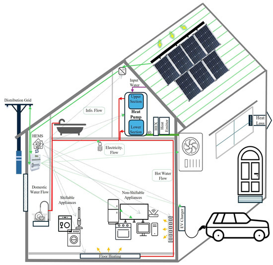
Figure 2.
The pilot house with various energy and communication elements.
The proposed DR model is implemented over selected days throughout the year to capture the impacts of various seasons, weather, and other factors. A random day from the second half of each month in 2024 is chosen to represent external temperature, solar radiation, and electricity prices. This selection method aims to provide a representative snapshot of seasonal variations and to highlight the interaction of cost-comfort trade-offs in both hourly and daily resolutions. While the initial plan was to optimise year-round, limitations in data quality and availability for the pilot house necessitated this approach. Although it effectively captures general trends, there remains the potential for missing seasonal extremes. The study is conducted at an hourly resolution to manage computational burden and can also be adjusted to a 15 min resolution. The weather data necessary for model operation, particularly regarding the predictions of outside temperatures, is obtained from the Norwegian Climate Service Centre [65]. The hourly electricity prices are the Nord Pool’s day-ahead prices for the NO1 area in the Nordics [66], obtained from the ENTSO-E Transparency Platform [67]. It is worth mentioning that the model accounts for an electricity subsidy on purchases for Norwegian residential customers, which is applicable for every hour the electricity price exceeds 0.73 NOK/kWh (≈0.063 Euro/kWh) excluding value-added tax, which is 25% in this study [68]. This is reflected in the parameter (cep) for hourly electricity, which is derived from the initial (non-subsidised) electricity prices (cep,i) through Equations (51) and (52). In these equations, (cth,p) and (cc,r) are the threshold price for electricity subsidy and the subsidy portion of electricity price, respectively. Under this supportive scheme aimed at assisting households with high electricity prices, the government subsidises 90% of the electricity cost that exceeds this threshold. The values of the parameters used in the modelling are all presented in Table A1.
The occupied pilot house is equipped with a rooftop PV system with a peak capacity of 17 kWp and is connected to Home Assistant, which integrates the Forecast.Solar service to provide daily forecasts of PV energy production [69]. This integration generates these predictions by combining system-specific parameters (location, tilt, azimuth, and peak capacity) with historical irradiance data from the EU Photovoltaic Geographical Information System (PVGIS) and numerical weather forecasts [70]. Figure 3 illustrates the three input data sets for the HES optimisation model, including outside temperature, day-ahead electricity prices, and PV energy production for the selected days throughout the year.
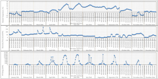
Figure 3.
Input data for the selected days, displaying variations in outside temperature (top), electricity prices (middle), and PV energy production (bottom).
The EV featured in this study is a Skoda Enyaq iV 80 (Škoda Auto a.s., Mladá Boleslav, Czech Republic), which offers a range of approximately 500 km and possesses a battery capacity of around 80 kWh [71]. Considering the reported average annual usage of 16,840 km for EVs in Norway [72] and the range of the considered EV, the model assumed a daily electricity consumption of approximately 7 kWh. To meet this daily requirement assumed in the day-ahead scheduling model, a standard 3.5 kW home EV charger is used, capable of charging the vehicle’s required daily energy need in approximately 2 h. It is assumed that the EV is not connected to the charger from 8:00 until 15:00. During the remaining intervals, the EV is kept connected to the charger to employ V2H technology, enabling bi-directional energy flow to provide support to the grid or home during peak demand periods. However, the manufacturer specifies that the V2H capability over the vehicle’s lifetime is limited to 4000 h, which corresponds to a total energy of 10,000 kWh. This limitation is considered by the maximum daily discharging time constraint in the HES optimisation [73].
Energy consumption for both shiftable and non-shiftable appliances, as depicted in Figure 2, is assessed using the Energy Use Calculator [74]. Table 3 provides an overview of the assumed energy usage of various appliances and the required operational times for each type in the pilot house. Based on the daily energy usage data in Table 3, the fridge, stove, microwave, LCD TV, and vacuum cleaner predominantly align with mid-class (B) energy efficiency appliances. This is based on comparisons with the official EU Product List for Energy Efficient Products, which is governed by Ecodesign and energy labelling regulations [75].
Table 3.
Energy usage for shiftable and non-shiftable appliances.
The thermal system data is predominantly sourced from the extensive study detailed in [38]. The power levels for the upper and lower sections of HPWH are 3 kW and 2 kW, respectively. The electricity demand for domestic hot water scenarios is calculated by evaluating volumetric flow rates and usage duration, with shower and faucet temperatures defined at 40 °C and 50 °C, respectively. These calculations are based on the NS 3055:1989 standard for dimensioning water systems in buildings, adapted from the Standard Regulations for Sanitary Facilities by the Nordic Committee for Building Regulations [76].
While the case study takes actual values from day-ahead forecasts of weather, PV production, and electricity prices, it should be noted that forecast errors may affect the actual operation of the HES. Moreover, the assumption of fixed daily EV electricity consumption and consistent connection intervals simplifies the model and facilitates comparisons among different days of the year, but it limits our ability to capture the full variability of real user behaviour. As highlighted in recent research, consumer responses to DR signals are inherently uncertain and influenced by behavioural, social, and contextual factors [77]. These include comfort, trust, intrinsic and extrinsic motivators, and individual comfort preferences, which can significantly impact the flexibility and effectiveness of DR programmes. Advanced approaches such as stochastic or robust optimisation explicitly account for such uncertainties [44], but these were outside the present scope. This work focuses on demonstrating the flexibility potential of an all-electric household while evaluating the cost–comfort trade-off. It also recognises that integrating forecast uncertainty and behavioural variability into the model represents an important avenue for future research.
The model was developed and solved as a MIP problem utilising the General Algebraic Modelling System (GAMS), which provides a robust framework for effective optimisation [78]. The SCIP solver was employed for solving the MIP formulation, known for its efficiency and advanced capabilities in managing complex optimisation problems [79]. The simulation was conducted on a Dell laptop (Dell Technologies Inc., Round Rock, TX, USA) equipped with an Intel i7-12700H processor (Intel Corporation, Santa Clara, CA, USA) and 16 GB of RAM. The maximum simulation time for a scenario within a single day was approximately 160 s, while the counts of total variables and total equations in the optimisation model were 837 and 1009, respectively.
4. Results and Discussion
The proposed price-based DR approach established a model for evaluating the trade-off between cost and comfort within a real-world smart home environment in Norway that incorporates PV production and e-mobility. This study addresses various aspects of the evaluation, organised into two primary categories. The first category focuses on an hourly perspective of energy management at an hourly resolution, examining how thermal, non-thermal, and e-mobility demands are met. The second category offers an extended overview of the DR model’s performance over selected days in different months, analysing its economic impact and user comfort under various tariff structures.
4.1. Hourly Analyses
This study focuses on implementing DR in a pilot Norwegian household that represents Northern European regions characterised by long winters and moderate summer temperatures, where air conditioning is unnecessary. In this case study, the flexibility potential of various electricity demands is examined to determine how the proposed HES optimises cost and comfort according to user preferences across the sampled days of the year.
In this regard, two out of the twelve sample days are discussed, one representative summer day and one representative winter day, to illustrate how seasonal and weather variations impact the model performance. For this analysis, 24 June (24-Jun) and 22 December (22-Dec) are selected, focusing on the scenario that prioritises cost over user comfort under the current Norwegian electricity billing model. The performance of this DR model in scheduling various electricity demands based on the multiple varying inputs for the aforementioned two days shown in Figure 4 will be discussed.
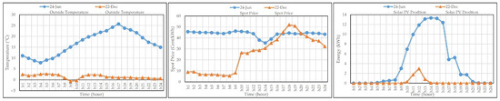
Figure 4.
Input parameters for the two selected days in June and December: (Left) Outdoor temperature, (Middle) Electricity price, and (Right) PV energy production.
4.1.1. Thermal Performance
In the thermal system, both water heating and space heating are scheduled based on key inputs, including outside temperature, electricity price, and user heating needs and preferences. In this model for energy consumption management of HPWH, the upper section for domestic water heating and the lower section for space heating are addressed separately.
- Water temperature in the HPWH’s upper section: To evaluate the behaviour of the upper section of HPWH, a fixed domestic hot water usage pattern is considered throughout different days of the year, as shown in Figure 5. This assumption allows for the comparison of the cost-comfort trade-off across various days in the prolonged analysis, although it may not effectively reflect real-world variability. While there are varying usage patterns and associated uncertainties, the primary aim of this study is to analyse the economic and flexibility potential.
- The optimisation results illustrated in Figure 6 highlighted the effective management of water heating to guarantee hot water availability based on the demand pattern in Figure 5. On 24 June, the HES prevented the activation of the upper section during the peak pricing period from 17:00 to 21:00 by utilising preheating between 13:00 and 16:00, as well as from 5:00 to 6:00 to meet morning hot water demand, as indicated in Figure 6.
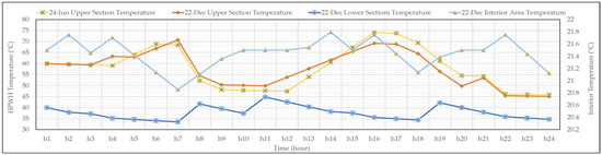 Figure 6. Temperature adjustments in the upper and lower sections of HPWH and the interior area.
 - On 22 December, solar capture was maximised during the peak production period, particularly starting at 13:00, to meet hot water needs throughout the day. However, as shown in Figure 6, the greater price variation throughout the day led to notable differences compared to 24 June. Specifically, from 14:00 onwards, as prices began to surge, the HES aimed to keep the temperatures lower.
- Water temperature in the HPWH’s lower section: Evaluating the behaviour of the lower section of HPWH in connection with the space heating system is essential for maintaining the desired temperature range to meet thermal needs. This evaluation requires consideration of the stored heat energy within the building. It should also be noted that space heating is assumed to be turned off during the summer months, from May to September.
- The lower section has a smaller water capacity, which reduces flexibility compared to the upper section. However, on 22 December, the HES has still room to optimise activations to minimise electricity costs and maximise comfort. This is particularly evident during the morning peak pricing from 8:00 to 10:00 and the evening peak pricing from 21:00 to 23:00, when activations are avoided, as illustrated in Figure 6.
- Air temperature in the interior area: The outdoor air temperature significantly impacts the optimisation of thermal systems by directly influencing the building’s heat loss rate. This, in turn, affects indoor conditions, as higher heat loss requires more heat to be injected. The results effectively display these connections. On 22 December, during the periods leading up to the significant peak pricing from 16:00 to 21:00, and while PV energy production is available from 11:00 to 13:00, the system raised the indoor temperature in preparation for the upcoming peak price interval. Conversely, as depicted in Figure 6, the management system lowers the temperature during the evening peak pricing interval. By utilising the thermal capacity of indoor air as a form of thermal storage, similar to the capacity of water in the tank, enables the system to fully leverage PV energy production while responding to fluctuations in electricity prices. Figure 6 illustrates the adjustments made to the temperatures in the upper and lower sections, as well as the interior area, to achieve the lowest costs while maintaining comfort and convenience over the selected days. The HES restricts the temperature of each element to predefined limits, with the hot water temperature in the tank set between 45 °C and 75 °C, and the interior area temperature set between 19 °C and 24 °C.
- To illustrate how the thermal system responds to varying inputs, the behaviour of the upper section of HPWH in supplying domestic hot water is analysed for 22 December. Two cases, defined in Table 4, were examined under nearly identical operating conditions, differing only in the electricity price input used in the optimisation model. In the first case, the hourly variable electricity price was applied, whereas the second case employed a fixed price calculated from the average of the day’s variable prices. This distinction is chosen because the demand profile of the thermal system remains largely unchanged across the two cases, apart from minor variations due to tank heat losses to ambient environment, while the cost of delivered energy varies significantly with the electricity price profile. Table 4 presents the hourly cost distribution for the HPWH’s water-heating operation under both pricing schemes. A comparison of the total daily electricity costs for water heating shows a 4.82% increase in total energy expenditure when a fixed electricity price is assumed. This difference exemplifies an energy-saving potential of thermal system through optimised thermal storage management.
Table 4. Water heating cost comparison in euros for 22 December: Case 1 based on hourly varying electricity prices, while Case 2 is based on the fixed electricity price calculated using the average of variable prices for the day.

Figure 5.
Domestic hot water demand pattern, comprising shower hot water usage and faucet hot water usage.
4.1.2. Non-Thermal Appliances and E-Mobility Performance
The non-shiftable appliances do not offer any flexibility and need to be supplied at predetermined intervals. In contrast, shiftable appliances can be optimally activated based on input data and preferences to achieve the lowest cost and highest comfort. In this study, these are the high-power appliances, such as the dishwasher, laundry appliances, and vacuum cleaner, which can provide practical, real-world flexibility.
The participation of EVs in implicit DR relies on two key aspects of charging and discharging. Given the high-power rate of EV charging, the HES generally allocates charging to the most cost-efficient intervals, capturing lower electricity prices, and maximising PV energy use based on the connection status. In this study, it is assumed that EV usage follows a consistent pattern throughout the selected days, aligning with typical use for commuting during working hours, which comes with specific electricity demands for mileage. The V2H capability are integrated into this model, allowing the EV to function as a storage for enhancing energy flexibility. However, this capacity is constrained by total discharging limits over the vehicle’s lifetime, as well as the efficiencies of charging and discharging in real-world scenarios. The HES manages the scheduling of charging and discharging as shown in Figure 7.
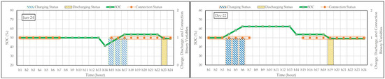
Figure 7.
SOC, charging, discharging, and connection status for 24 June (left) and 22 December (right).
On 24 June, when there is considerable PV energy production throughout most of the day, the system postpones charging to the afternoon, right after returning home, to capture and store solar energy. Based on Figure 7, the stored electricity is then discharged in the late evening. On 22 December, with limited PV energy production and considerable variations in electricity prices alongside higher heating demand, the HES allocates charging before departure and during the low electricity peak periods. On the other hand, it discharges during the evening peak prices to achieve maximum cost savings, according to Figure 7. The presence of an efficiency factor that causes energy loss during the charging and discharging limits the V2H capacity, particularly when cost is the primary consideration. In contrast, scenarios where comfort is the main objective see greater involvement with V2H, up to the manufacturer’s limit per day. While frequent V2H cycles can contribute to battery degradation, such implications are generally assessed over long-term usage. This study focuses on an hourly analysis within the manufacturer’s specified limits designed to prevent significant degradation. Therefore, it is expected that the battery does not experience notable deterioration during the time scope of this analysis.
This analysis provides insights into how each demand category contributes to overall energy consumption throughout the day. As illustrated in Figure 8, the HES aligns with the varying electricity prices and hourly PV energy production shown in Figure 4. On 24 June, the day features a relatively flat electricity price, with a decrease from 13:00 to 16:00, coinciding with strong PV production. The management system utilises this opportunity to activate several electricity demands during this interval. On 22 December, the lower electricity prices in the morning shift most electricity demands to the period before 10:00, along with some during the noon PV energy production interval, as depicted in Figure 8.
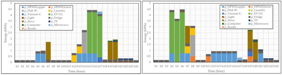
Figure 8.
Optimised hourly schedule of various household electricity demands with different colours in the diagrams, including appliances, HPWH, and EV charger for 24 June (left) and 22 December (right).
Figure 9 demonstrates the model’s effectiveness in optimising electricity consumption, production, and transactions with the main grid. A key insight is the observable relationship between total demand, PV energy production, and electricity prices. The DR model utilises flexibility by accommodating high-power non-shiftable loads at user-preferred times, even during high evening electricity prices.
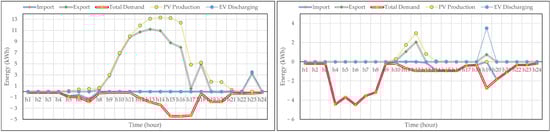
Figure 9.
Total power bought from and sold to the grid and total power demand for 24 June (left) and 22 December (right).
The negative values for grid energy reflect surplus electricity after household self-consumption, which is subsequently sold to the grid. However, it is fundamental to understand that the Norwegian billing system does not provide equal payment rate for electricity sold to the grid compared to electricity purchased. Buying electricity from the grid incurs additional costs compared to selling, including a fixed monthly fee, several add-on charges from the grid provider, and VAT. These additional expenses associated with selling, compared to buying, make selling electricity less economically comparable and instead indirectly encourage self-consumption of produced PV energy. This outcome underscores the opportunity for alternative local energy trading schemes, which can be developed through adjustments to the grid tariff models. These possibilities are discussed in the subsequent section on prolonged analysis.
4.2. Prolonged Analyses
Analysing the proposed implicit DR approach over extended time horizons and scenarios within real-world pilot houses can provide valuable insights for policymakers and energy stakeholders, particularly in supporting the development of solar-integrated smart homes. Four scenarios focusing on cost and comfort priorities are outlined in this paper. They are designed to evaluate the performance of the proposed energy management process over multiple selected days throughout the year. The analysis assesses how grid tariff designs and prioritising comfort affect cost savings, exploring how effective policy adjustments can benefit prosumers. This economic assessment also includes measuring self-supply indicators based on the self-consumption and self-sufficiency of PV installations under varying conditions throughout the year. The scenarios (Sc) are structured as follows:
- Sc1—Variable Pricing: This serves as the baseline scenario that incorporates the current household electricity billing model. It reflects the dynamic pricing approach as Norwegian grid tariff model, similar to those in many other countries, which includes various components based on variable electricity prices from the day-ahead market, fixed charges, and public fees.
- Sc2—Fixed Pricing: This scenario closely resembles Sc1, with the key distinction being its reliance on a fixed price rather than varying electricity prices. A fixed rate of 0.4 NOK/kWh (≈0.034 Euro/kWh), excluding VAT, is proposed by the Norwegian government under the designation “Norgespris” to ensure predictable and stable electricity costs for households [80]. The establishment of a fixed price eliminates the ability of HES to react to fluctuations in electricity prices. As a result, DR programme becomes reliant solely on other variable factors, such as PV energy production and outdoor temperature. This scenario effectively removes price sensitivity as the main inout for the implicit DR programme, serving as a benchmark among all scenarios where HES exhibits minimal reaction to varying inputs. While complete removal of this reaction is not feasible within this pilot study, previous research has evaluated household participation in the demand-side management programme across three pre-defined engagement levels [38].
- Sc3—eNeighbourhood Pricing: This scenario builds upon Sc1 by focusing on Energy Neighbourhoods (eNeighbourhoods) that aim to indirectly incentivize the sale of electricity within local communities. The concept of eNeighbourhoods in this study is rooted in the idea of Positive Energy Neighbourhoods, defined as areas that produce more energy than they consume, resulting in an energy surplus that can be exported to the grid or stored [81]. This approach shifts the focus from individual energy-efficient buildings to managing energy at the neighbourhood or district level. Since the pilot house produces more annual PV energy than it consumes in Sc1 across selected days, it can be scaled to a neighbourhood level to facilitate local energy trading among households. The current Norwegian electricity billing model for selling produced electricity to the grid is not economically comparable to purchasing electricity from the grid. To promote investment in household PV beyond the purpose of self-consumption in Sc1 by making buying and selling rates close to each other, this paper examines the elimination of specific terms in the cost objective of Equation (1) to reduce the economic asymmetry mentioned. The idea is to enable and encourage local electricity trading. Local electricity trading can potentially alleviate utilisation of grid capacity at distribution level close to end-user. One can argue that as a result, DSOs costs will also reduce, which justifies a remodelling of grid fee design [82]. This scenario examines the impact of eliminating the add-on parameters associated with (cd) (the consumption fee for the grid supplier) and (cs) (the charge from the energy supplier) as a subsidy mechanism on grid usage. Dropping these two terms can provide insights into the maximum economic potential by mitigating the grid usage factor from the energy bill. Similarly, several European projects have focused on the removal or reduction in grid-related fees. Austria’s Grid Singularity Exchange adjusts tariffs for peer-to-peer trading, minimising grid fees to enable dynamic local markets [83]. Portugal’s Miranda do Douro Renewable Energy Community, reduces network charges for shared solar energy, encouraging local use [84]. In Norway, high shares of EVs and HPs at the end-consumer level result in grid charges accounting for about one-third of electricity prices [85]. Norwegian authorities recognise the need for local flexibility incentives, but there are currently no specific regulatory drafts in place [85]. This concept lays the groundwork for future research aimed at developing a multi-layer market structure for electricity transactions. Similarly to Austria’s regulatory framework, which allows households in renewable energy communities to pay only grid charges associated with their specific levels, this structure minimises additional trading costs [85]. This can incorporate varying reduction stages of the aforementioned terms in the proposed model based on local energy engagement between producers and consumers.
- Sc4—Comfort Priority: This scenario is entirely different from the other three, which prioritise cost as the primary objective in their multi-objective optimisation, followed by comfort as the secondary objective. In contrast, this scenario places user comfort and convenience as the top priority, with cost considered as the second priority.
The scenarios are compared based on the following criteria: cost, comfort, and self-supply, which are detailed in the following subsections.
4.2.1. Cost Analysis
This analysis examined the effects of different grid tariff designs and comfort on cost savings for the pilot household through price-based DR. The four scenarios discussed above are incorporated into different optimisation problems and are run for each scenario on selected days throughout the year. The analysis shows that the optimal economic outcome values can be both positive and negative, indicating differing profits for various days of the year. This variation arises from calculating the total daily profit (defined as revenues minus costs) by accounting for electricity sold back to the grid against electricity purchased from the grid, primarily from PV energy production. Figure 10 illustrates how these profits for the four scenarios are distributed across the year. Accordingly, positive profit values occurring mainly in the summer indicate that revenues exceed costs on those selected days, whereas the opposite is true for the rest of the year.
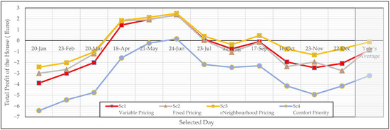
Figure 10.
Optimal profit values of the proposed DR model with PV production under different scenarios across selected days of the year. The shaded region in the diagram indicates the annual average values.
Focusing on the three cost-priority scenarios (Sc1, Sc2, and Sc3) in Figure 10, a similar profit trend is followed throughout the selected days of the year, along with some notable differences. In Scenario Sc1, which reflects the current electricity billing mechanism based on variable pricing, the outcomes are similar to those of Sc2, an adjusted version based on fixed pricing. Based on Figure 10, it is evident that Sc2 does not necessarily result in a higher electricity profit for all the months; for instance, in the days in August, October, and December, the results indicated that fixed pricing incurred comparable or even higher costs than variable pricing. The annual average profit is derived from the average profit values of twelve sampled days across the year. Transitioning from Sc1 to Sc2 resulted in a 13.5% increase in this annual average profit, with the average electricity price for the selected days being around 0.5 NOK/kWh (≈0.043 Euro/kWh). The fixed price of 0.4 NOK/kWh (≈0.034 Euro/kWh) is advantageous for prosumers purchasing electricity from the grid. These findings provide a clear perspective for prosumers regarding the extent of improvement they can expect from switching from variable electricity prices to fixed prices. In addition, Sc3 includes an adjustment to the grid tariff model to facilitate local electricity trading, allowing for a comparison with the other two cost-priority scenarios. As depicted in Figure 10, this scenario effectively achieved the highest profit compared to the other scenarios, nearly offsetting the annual average costs with the annual average revenue. Transitioning from Sc1 to Sc3 is expected to result in an 87% increase in the annual average profit. This is indeed an upper bound of the maximum reduction, considering only the consumer’s side. To achieve comprehensive tariff price optimisation, one can design a model to generate tariff prices based on a portion of the aforementioned reduction through a multi-layer structure while encouraging consumers to shift their consumption from on-peak ToU to other time-of-use periods (mid-peak, off-peak), all while ensuring the profitability of the system operator at a certain level [86]. This highlights how grid tariff adjustments for neighbourhood electricity trading can benefit prosumers.
A significant observation in Figure 10 is that when transitioning from the cost priority scenarios to the comfort priority scenario (Sc4), there is a substantial jump in costs, resulting in an almost fourfold decrease in the annual average profit. This change highlights how prioritising comfort over cost in a price-based DR can lead to significantly different profit for a household. Additionally, Figure 10 shows that summer days exhibit lower costs and positive profits due to two main factors: considerable PV energy production during long summer days and the deactivation of space heating systems. On the specific day of August 21, which represents a cloudy day with relatively low PV energy production and very low electricity prices as shown in Figure 3, the system ended up with a negative profit value, despite being in summer and having space heating turned off. The selected days in July and September experienced a balance between costs and revenues in the cost-based scenarios in Figure 10, similar to the patterns observed in May and June for the comfort priority scenario.
Figure 10 illustrates the profit of the pilot house with photovoltaic (PV) energy production, functioning as a prosumer by selling excess energy back to the grid to generate revenue. In contrast, when considering the same house without a PV installation—primarily purchasing electricity from the grid—a markedly different economic outcome is revealed, reflecting only costs, as shown in Figure 11. In this scenario, selling is limited to V2H, and buying depends largely on total daily electricity demand. Among the three cost-based scenarios, space heating is the key variable in electricity demand, correlating with outdoor temperatures throughout the selected days of the year. Notably, Sc1 and Sc2 show nearly equal annual average costs for electricity, indicating that the proposed fixed pricing does not necessarily benefit consumers compared to variable pricing. The lower costs during the summer months evident in Sc1 and Sc3 are influenced by typically reduced electricity prices and fluctuations, as illustrated in Figure 3. In the absence of a price factor, as shown in Sc2, cost variability across different days is significantly reduced.
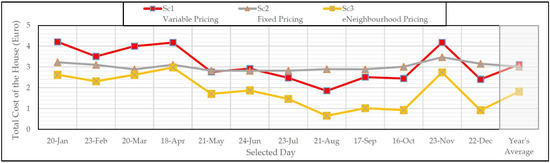
Figure 11.
Optimal cost values of the proposed DR model without PV production under different scenarios across selected days of the year. The shaded region indicates the annual average values.
The results for fixed price steps illustrate that the optimal fixed price varies throughout the year based on the peak power demands of the household. This variation reflects how seasonal factors and key model inputs influence peak power demand to minimise electricity costs. Notably, when moving from Sc1 to Sc4, where comfort is prioritised, the fixed price step is significantly higher. This indicates that the simultaneous activation of various electricity demands can enhance comfort but also lead to considerably increased costs.
4.2.2. Comfort Analysis
This section of the results discusses the critical topic of comfort and convenience in DR optimisation, which is highly valued by households, according to the conducted surveys [87]. While three scenarios prioritise cost, Sc4 in contrast focuses on comfort. The comfort objective comprises three main elements: space heating (interior area temperature), water heating (domestic hot water temperature), and e-mobility (EV’s SOC). In Figure 12, the three graphs illustrate how the optimisation problem addresses user comfort across different days throughout the year. Each graph presents four scenarios, and it is evident that Sc4, associated with the comfort priority scenario, stands out from the others by exhibiting the highest values. The average annual comfort value for Sc4 was 31.3%, 20.9%, and 13.7% higher than the averages of the three cost-based scenarios for interior area temperature, domestic hot water temperature, and EV’s state of charge (SOC), respectively. This distinction arises because, unlike the cost-based scenarios where comfort indicators are not prioritised in the first-layer optimisation, Sc4 places comfort as the highest priority. Overall, the three cost priority scenarios demonstrate similar and close trends in Figure 12. Notably, among these cost priority scenarios, Sc2 achieves the highest average comfort levels across all three categories: space heating, water heating, and e-mobility. With fixed-price DR, the main variable element of price is eliminated. This allows only variations in PV production and outside temperature to affect comfort, while the variations among the cost priority scenarios remain closely aligned. The top graph in Figure 12 addresses space heating, which is inactive during the summer months.
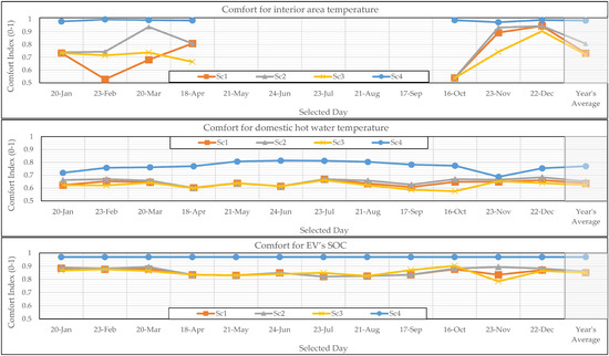
Figure 12.
Optimal values of normalised comfort indices across selected days of the year for different scenarios: (top) space heating, (middle) water heating, and (bottom) e-mobility. The shaded regions indicate the annual average values.
4.2.3. Two-Layer Optimisation Assessment
The proposed Lexicographic approach solves the multi-objective optimisation problem in a sequential manner. In the second layer of the optimisation problem, a constraint is introduced to maintain the optimal value of the first objective while optimising the second objective. The performance of the proposed method can be evaluated by comparing the objective values of the second layer with the calculated value of the same objective function as a function of optimal values from the first layer. The extent of change between the two layers for both cases is illustrated in Figure 13. This figure illustrates the improvements in each of the comfort indicators and profit in both the cost-priority (Sc1) and comfort-priority (Sc4) scenarios, respectively. In the cost-priority scenario, larger values for comfort are achieved when optimised in the second layer compared to the calculated comfort parameter in the first layer of Sc1. Conversely, bigger values for profit (smaller values for cost) are obtained when optimised in the second layer compared to the measured profit parameter in the first layer of Sc4. In Sc1, the objective is to maintain the optimal profit objective value achieved in the first layer through the second layer, while also improving the second objective; a similar approach is observed in Sc4.
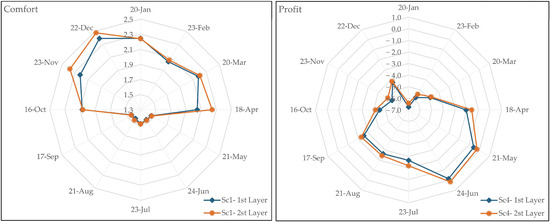
Figure 13.
Changes in the optimal objective values of the second layer and the associated objective function calculated from the first layer across selected days of the year: (left) comfort indicator and (right) profit.
In addition, another aspect that can be measured is the change in decision variables across the two layers of optimisation. To further analyse what occurs between the two layers, an example from Sc4 for the day of 21 May is presented. In this case, the demand for the two layers in terms of shiftable appliances takes various activation intervals, resulting in different dispatches of the total demand across the hours of the day. A notable point is that, since comfort is the highest priority in this scenario and is optimised in the first layer, all comfort indicator values must be preserved in the second layer. Consequently, there is no room for changes in the variables associated with water heating and EV charging to maintain the same comfort level. Therefore, only the shiftable appliances are affected. This leads to a different profile for the power purchased from the grid and the power sold back to the grid (pb and ps) across the two layers, with a reduction of 22% in purchased power and 7% in sold power when comparing the second layer with the first layer of optimisation. Overall, this results in a slight increase in profit in the second layer compared to the first layer, as shown in Figure 13. On the other hand, for the same day of 21 May in Sc1, the main changes occur in the distribution of power purchased from the grid and the power sold back to the grid. The activation status of the EV charger also undergoes minor differences resulting in a small change in the total comfort value in Figure 13. Another noticeable change occurs during winter days, where the inclusion of space heating in the model leads to greater comfort variations between the two layers of optimisation. This leads to improved optimised comfort values in the second layer compared to the measured comfort indicators in the first layer of the cost-priority scenario, while preserving the optimal profit value.
4.2.4. Self-Supply Analysis
As discussed in the section on multi-objective optimisation, two self-supply measures are defined as indicators of self-consumption and self-sufficiency. These indicators are similar in that they allocate PV energy used over total PV production and total demand, respectively. These metrics measure how different scenarios influence the PV capture capability of the household. This is beneficial, as mentioned earlier, since selling electricity to the grid is not as cost-effective as self-consumption.
The choice of the highest priority objective between cost and comfort impacts the total electricity demand of the household. When comfort is the highest priority, as in Sc4, the primary areas of increased demand are space heating and the SOC of batteries. This focus on comfort and convenience limits flexibility in deviating from the desired temperature or battery charge, resulting in higher electricity demand, as illustrated in Figure 14. Moving from Sc1 to Sc4 leads to a 65% increase in annual average demand, rising from 31.1 kWh to 51.6 kWh, while the annual average PV energy production is 37.9 kWh. This indicates that by prioritising comfort over cost, the household shifts from self-sufficiency to grid dependency for some days, highlighting the importance of this trade-off. Sc2 experienced an annual average total demand similar to Sc1, while Sc3 showed an increase of 19.9% from Sc1. Sc3 also achieved a significant 30.9% increase in the annual average energy sold to the grid, translating to an additional 7.95 kWh in sales and a 6.18 kWh rise in demand. Table 5 provides a detailed analysis of the demand and net energy traded with the grid (sold energy minus purchased energy) under the two scenarios of Sc1 (variable pricing) and Sc3 (eNeighbourhood pricing). Beyond the annual average values, the considerable gap between the demands of the two scenarios is also partially reflected in the relatively smaller gap in traded energy with the grid, especially on the selected winter days of 20-Jan, 20-Mar, 17-Sep, 16-Oct, 23-Nov, and 22-Dec. This indicates that the proposed eNeighbourhood pricing increases the overall demand of households due to a lower final electricity cost, a trend that is especially pronounced during winter months when heating demands are high, and PV production significantly drops. The increased reliance on grid energy during winter days makes this tariff reduction more appealing for boosting consumption. However, HES limits the increase in the traded energy to avoid escalating costs resulting from increased demand in Sc3 compared to Sc1. This is similar to the observation that the average annual demand of households under Sc3 does not exceed the annual solar production in Table 5.
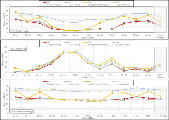
Figure 14.
Optimal results of four scenarios for total energy purchased from the grid (top), total energy sold to the grid (middle), and total electricity demand of the household (bottom) across selected days of the year. The shaded regions indicate the annual average values.
Table 5.
PV production, demand, and net energy trade with the grid for the selected days under variable and eNeighbourhood pricing scenarios.
The two graphs of transactions with the grid in Figure 14 provide insights into the differences among the four scenarios. The total sold energy exhibits a similar trend across all scenarios, with the annual averages for Sc3 and Sc4 being nearly identical, as well as those for Sc1 and Sc2. However, Sc1 and Sc2 have lower values, approximately 23% less than those of Sc3 and Sc4. The total energy purchased from the grid exhibited greater variations among the four scenarios across selected days of the year, with Sc4 generally showing the highest values. This is because when cost is not the primary objective: First, HES shifts its focus from cost-based allocation of electricity demands solely on captured PV production to a more comfort-oriented activation schedule, maximising PV energy sale potential to the grid. Second, HES overlooks the costs associated with charging and discharging EV, engaging it more frequently through V2H, which also enhances grid sales potential. The annual average bought energy values in Figure 14 illustrate that Sc4 and Sc3 have higher values of 121% and 59%, respectively, compared to the nearly identical values of Sc1 and Sc2. These results regarding transactions with the grid indicate that while variable pricing and fixed pricing do not offer significant annual average values, eNeighbourhood pricing can lead to an increase in demand. Additionally, prioritising comfort may result in a substantial amount of energy purchased from the grid and lower self-supply indicators.
Figure 15 compares the self-consumption and self-sufficiency indicators across the four scenarios. Both indicators reach higher values under cost-priority operation, whereas prioritising comfort in Sc4 results in a 16% reduction in annual average self-consumption and a 50.1% decline in self-sufficiency. These outcomes can be explained by changes in both the numerator and the denominator of the indicators. In the case of self-consumption (fc), the numerator, representing the portion of PV energy used directly within the household, decreases when comfort-oriented scheduling shifts energy use away from PV-abundant hours, while the denominator, the total PV generation, remains constant, lowering the ratio. For self-sufficiency (fs), the same reduction in PV utilisation decreases the numerator, but the effect is magnified by an increase in the denominator, as total household demand grows due to enhanced space heating and water heating comfort requirements. This combined influence explains the more pronounced decline in self-sufficiency compared to self-consumption.
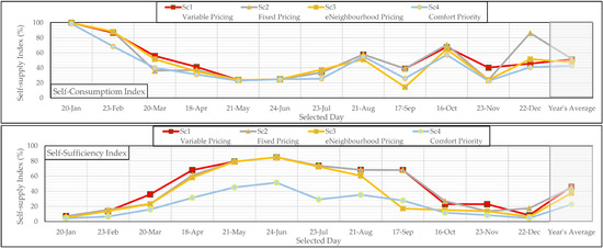
Figure 15.
Self-supply indicators from PV installations across selected days of the year: (top) self-consumption and (bottom) self-sufficiency. The shaded regions indicate the annual average values.
Seasonal variations further reinforce these differences. During winter, limited solar availability and high heating demand simultaneously reduce the numerator and enlarge the denominator of fs, leading to a substantial fall in self-sufficiency. In contrast, summer conditions, with higher PV output and lower demand, improve both indicators, although these gains are insufficient to offset winter deficits in the annual average. These results confirm that the 50.1% reduction in self-sufficiency for Sc4 is primarily driven by the seasonal imbalance between PV generation and thermal demand. From a broader perspective, these findings reveal a clear trade-off between user comfort, renewable energy utilisation, and grid dependency. Comfort-priority operation improves indoor conditions but increases electricity imports during low-PV periods, reducing household energy autonomy. Policy measures tailored to seasonal demand variations, along with targeted incentives for seasonal flexibility, can optimise PV utilisation and enhance energy self-reliance. For example, achieving up to 99.1% cooling energy coverage using solar heat has been demonstrated in Southern Italy [88]. Additionally, subsidies for advanced thermal storage systems, such as hybrid polygeneration setups with payback periods ranging from 8.2 to 24 years depending on location [89], can contribute to effectively balancing comfort and energy independence. Implementing these strategies could mitigate the observed 50% decrease in self-sufficiency by reducing grid reliance during low PV generation months in winter while maintaining occupant well-being through sustained indoor comfort and cost savings.
The hourly analysis revealed the scheduling decisions that influenced the aggregated outcomes observed in the prolonged analysis. It evaluated the impact of the proposed DR model in scheduling various electricity demands based on the multiple varying inputs for the selected day. For example, preheating of indoor spaces and hot water before evening peak prices reduced reliance on costly electricity during high-tariff hours, which accumulated into the cost savings and improved self-consumption observed across the year. Similarly, the strategic timing of EV charging to coincide with periods of high PV generation or low electricity prices underpinned the higher summer profits and improved comfort indices reported for Sc4. These representative daily schedules thus illustrate how optimisation achieved a balance between cost and comfort, while the prolonged analysis quantified their cumulative impact over several months. Additionally, the prolonged analysis assessed how grid tariff designs and prioritising comfort affect cost savings and self-supply from PV installation. The two perspectives illustrated not only how scheduling decisions were made on an hourly basis, but also why these decisions mattered for long-term household performance.
5. Conclusions
This study evaluated a novel Home Energy Scheduler (HES) designed for all-electric residential buildings, emphasising the interplay between cost effectiveness and occupant’s comfort. By developing a sequential multi-objective optimisation model, the research provided a framework for effectively prioritising competing objectives in household energy management. This approach integrated diverse electricity demands, including thermal, non-thermal, and e-mobility, along with V2H capabilities. This study contributed practical insights into efficient energy consumption, enabling households to optimise their reliance on PV energy production based on electricity prices and outside temperatures. This geographically adaptable model assessed the flexibility potential of Nordic households by examining both electricity demands and PV production at the intersection of profit and comfort. Additionally, it highlighted the significance of diverse grid tariff designs and demonstrated how effective adjustments to local energy trading policies can enhance economic benefits for households.
The HES maintained water temperatures according to usage patterns and preferences, ensuring availability at the lowest cost. On the specific summer day, the HES effectively prevented activation of the thermal system during peak pricing by preheating water in the upper section in advance. Optimising the activation timing of appliances is essential, specifically scheduling high-power devices during the lowest cost intervals. The participation of EVs as flexible energy storage accounts for charging at cost-effective times based on PV production and electricity prices. On the specific summer day, charging was postponed to late afternoon to effectively utilise solar energy, while on the winter day, it was scheduled during lower price periods to minimise costs.
To investigate the impact of pricing schemes, grid tariff alternatives, and user preferences on the performance of the proposed implicit DR in the real-world pilot house, four scenarios were developed. These scenarios are compared based on their cost savings, comfort, and self-supply. The cost analysis assessed how different tariff structures impacted cost savings within the context of a price-based DR framework. Moving from variable pricing to fixed pricing resulted in an annual average reduction of 14% in costs, with fixed pricing proving advantageous for prosumers. The proposed eNeighbourhood pricing demonstrated the best economic performance, achieving an annual average reduction of 87% in total costs compared to variable pricing. Significant disparities between cost-priority and comfort-priority scenarios were observed, with the latter resulting in almost a fourfold increase in the annual average costs. The analysis highlights that fixed pricing does not always yield benefits compared to variable pricing.
The comfort analysis examined the importance of comfort in DR, compiling outcomes related to space heating, water heating, and e-mobility. The results showed that prioritising comfort consistently achieved the highest comfort values, with average annual comfort levels 31%, 21%, and 14% higher than the average of cost-based scenarios for interior area temperature, domestic hot water temperature, and EVs’ SOC, respectively. Among the cost-prioritised scenarios, fixed pricing provides the best average comfort levels across all categories, benefiting from fixed price, eliminating price fluctuations.
The self-supply indicators are introduced to evaluate how different scenarios influence the household’s PV self-supply. When comfort is prioritised, there is a notable increase in total electricity demand, primarily driven by space heating and EV. This leads to a 65% rise in the annual average demand in variable pricing in the cost priority scenario compared to the comfort priority scenario. Consequently, prioritising comfort results in decreased self-sufficiency, as indicated by a 16% drop in average self-consumption and a 50% fall in average self-sufficiency when moving from variable pricing compared to comfort priority. The self-consumption values are generally higher in summer due to increased PV production and lower demand, whereas self-sufficiency is greater in winter.
The findings emphasise the importance of adaptable pricing strategies and local trading policies in reducing grid dependency and improving household cost savings. Future research will prioritise neighbourhood modelling to scale demand-side management from single households to multiple homes. This approach enables further integration of social and psychological behavioural analyses, including user comfort. Concrete regulatory suggestions include implementing eNeighbourhood pricing frameworks through minimal market restructuring and by alleviating certain cost elements based on multi-layer grid structures for local energy trading. Together with economic analyses of investment costs and returns for solar-integrated all-electric households, these measures can enhance the adoption of rooftop PV, bidirectional EV chargers, and HPs. This study, however, relied on several simplifying assumptions, including the use of representative daily samples for each month, perfect day-ahead forecasts, and fixed EV charging behaviour. While these assumptions ensured model tractability and comparability, they limit the representation of behavioural and operational uncertainties. Future research should therefore expand the HES framework by incorporating stochastic or robust optimisation methods and predictive control strategies to better capture forecast errors and behavioural variability as the model scales to the neighbourhood level.
Author Contributions
Conceptualisation, M.A.; methodology M.A., M.B., J.N. and G.H.; software, M.A.; validation, M.B., J.N. and G.H.; formal analysis, M.A., M.B., J.N. and G.H.; investigation, M.B.; resources, J.N.; data curation, M.A. and J.N.; writing—original draft preparation, M.A.; writing—review and editing, M.B., J.N. and G.H.; visualisation, M.A.; supervision, M.B., J.N. and G.H.; project administration, M.B. and J.N.; funding acquisition, M.B. All authors have read and agreed to the published version of the manuscript.
Funding
This research was conducted within the PriTEM project, which is funded by the Faculty of Mathematics and Natural Sciences at the University of Oslo (UiO) and the Convergence Environment at UiO:Energy.
Data Availability Statement
All data used in the modelling for this study are presented in the article. Further inquiries can be directed to the corresponding author.
Acknowledgments
We would like to thank our colleagues at the interdisciplinary PriTEM project for their input and discussions. The authors take full responsibility for the content of this publication.
Conflicts of Interest
The authors declare no conflicts of interest. The funders had no role in the design of the study; in the collection, analyses, or interpretation of data; in the writing of the manuscript; or in the decision to publish the results.
Abbreviations
The following abbreviations are used in this manuscript:
| COP | Coefficient of Performance |
| CPP | Critical Peak Pricing |
| DESSI | Distributed Energy System and Security Infrastructure |
| DR | Demand Response |
| e-mobility | Electric Mobility |
| eNeighbourhood | Energy Neighbourhood |
| EV | Electric Vehicle |
| GAMS | General Algebraic Modelling System |
| HEMS | Home Energy Management System |
| HES | Home Energy Scheduler |
| HP | Heat Pump |
| HPWH | Heat Pump Water Heater |
| MILP | Mixed Integer Linear Programming |
| MIP | Mixed Integer Programming |
| MP | Measured Power |
| nZEB | Nearly Zero Energy Building |
| PV | Photovoltaic |
| Sc | Scenario |
| SOC | State of Charge |
| ToU | Time of Use |
| TR | Tiered Rate |
| V2G | Vehicle to Grid |
| V2H | Vehicle to Home |
Appendix A
The parameters required for the optimisation problem are provided in Table A1.
Table A1.
The parameters and their values to run the proposed DR model.
Table A1.
The parameters and their values to run the proposed DR model.
| Parameter | Description | Value | Parameter | Description | Value |
|---|---|---|---|---|---|
| cnet | Add-on fee for grid supplier for day consumption | 0.43 NOK/kWh (≈0.037 Euro/kWh) | ua | Temperature of environment around HPWH | 18 °C |
| Add-on fee for grid supplier for night consumption | 0.37 NOK/kWh (≈0.032 Euro/kWh) | uc | Cold water temperature entering HPWH | 10 °C | |
| cpro | Add-on fee for grid supplier for production | 0.05 NOK/kWh (≈0.004 Euro/kWh) | uw,d | Target temperature of HPWH’s upper section | 60 °C |
| cpub | Add-on fee for energy supplier | 0.06 NOK/kWh (≈0.005 Euro/kWh) | uu | Min. temperature in HPWH’s upper section | 55 °C |
| cfix | Monthly add-on fee for energy supplier | 39 NOK (≈3.33 Euro) | Max. temperature in HPWH’s upper section | 65 °C | |
| m | Billing period | 30 days | Max. temperature in HPWH’s upper section with solar input | 70 °C | |
| cvat | Value Added Tax | 0.25 | ul,−5 | Min. temperature in HPWH’s lower section at −5 °C outdoor temperature | 35 °C |
| lg | Fuse power limit (36 A) | 7.5 kW | Max. temperature in HPWH’s lower section at −5 °C outdoor temperature | 45 °C | |
| ms | Appropriately small value for linearisation | 1.0 × 10⁶ | ul,18 | Min. temperature in HPWH’s lower section at 18 °C outdoor temperature | 20 °C |
| mb | Appropriately big value for linearisation | 1.0 × 10⁻⁶ | Max. temperature in HPWH’s lower section at 18 °C outdoor temperature | 30 °C | |
| au | Surface area of the tank in HPWH’s upper section | 1.06 m2 | ur | Min. acceptable indoor temperature | 21 °C |
| al | Surface area of the tank in HPWH’s lower section | 2.73 m2 | Max. acceptable indoor temperature | 22 °C | |
| ςw | Heat capacity of water | 1.16 Wh/kg·K | ui,d | Desired temperature for indoor space | 21.5 °C |
| ςa | Heat capacity of air | 0.28 Wh/kg·K | uw,d | Desired temperature for hot water | 60 °C |
| hu | Hight of the tank in the upper section | 1.4 m | ui,r | Temperature range for indoor space | 3 °C |
| hl | Hight of the tank in the lower section | 0.5 m | uw,r | Temperature range for hot water | 20 °C |
| d | Diameter of the tank | 0.59 m | νs | Slope for linear relationship between COP and outdoor temperature | 0.075 |
| ωu | Volume of the tank in HPWH upper section | 224 m3 | ҝu | Intercept for linear relationship between upper COP and outdoor temperature | 2.125 |
| ωl | Volume of the tank in lower section of HPWH | 136 m3 | ҝl | Intercept for linear relationship between lower COP and outdoor temperature | 3.125 |
| ηu | Heat transfer from HPWH’s upper section | 1.1 W/m2·°C | ηv | Efficiency of EV charging and discharging | 0.95 |
| ηl | Heat transfer from HPWH’s lower section | 5.2 W/m2·°C | ev,us | EV’s electricity consumption for day’s drive | 7 kWh |
| ηi× ai | Thermal characteristic of the house as product of accumulated heat transfer coefficient and surface area | 100 Wh/°C | pv | Standard EV charger power rate | 3.5 kW |
| php,u | Power consumption rate of HPWH’s upper section | 0.75 kW (3 kWh) | cth,p | Threshold price for electreicty susbsidy | 0.73 NOK (≈0.062 Euro) |
| php,l | Power consumption rate of HPWH’s lower section | 0.5 kW (2 kWh) | cc,r | Subsidy portion of electricty price | 0.90 |
The absolute functions introduce nonlinearity, making them incompatible with MILP formulations in this optimisation model. This part of the Appendix A outlines the linearisation techniques employed to incorporate absolute functions within the comfort index calculations in Equations (2)–(4). As an example, the comfort indicator for space heating, defined in Equation (2), is transformed into Equation (A1).
Two positive variables, (zp) and (zn), are defined as auxiliary variables to reformulate the absolute function, according to Equations (A2) and (A3).
Substituting these definitions back into the comfort index for space heating yields a linear model. The same process is applied to the other two comfort indicators.
References
- Duguma, D.G.; Zhang, J.; Aboutalebi, M.; Zhang, S.; Banet, C.; Bjørkli, C.; Baramashetru, C.; Eliassen, F.; Zhang, H.; Muringani, J. Privacy-preserving transactive energy systems: Key topics and open research challenges. arXiv 2023, arXiv:2312.11564. [Google Scholar] [CrossRef]
- Sartori, I.; Wachenfeldt, B.J.; Hestnes, A.G. Energy demand in the Norwegian building stock: Scenarios on potential reduction. Energy Policy 2009, 37, 1614–1627. [Google Scholar] [CrossRef]
- Patrick Jowett (pv Magazine). Norway Records 148.68 MW of New Solar in 2024. Photovoltaics Markets and Technology 2025. Available online: https://www.pv-magazine.com/2025/01/09/norway-records-148-68-mw-of-new-solar-in-2024/ (accessed on 9 October 2025).
- Statnett. Increased Consumption Results in a Negative Norwegian Energy Balance From 2027. 2023. Available online: https://www.statnett.no/en/about-statnett/news-and-press-releases/news-archive-2022/increased-consumption-results-in-a-negative-norwegian-energy-balance-from-2027/ (accessed on 8 October 2025).
- European Commission; Directorate-General for Energy. European Union Energy and Transport in Figures; Office for Official Publications of the European Communities: Luxembourg, 2001. [Google Scholar]
- Solheim, H.; Vatne, B.H. Home Energy Conversion can be a Net Cost for the Average Household; Staff Memo; Norges Bank: Oslo, Norway, 2024. [Google Scholar]
- Sadeghi, H.; Ijaz, A.; Singh, R.M. Current status of heat pumps in Norway and analysis of their performance and payback time. Sustain. Energy Technol. Assess. 2022, 54, 102829. [Google Scholar] [CrossRef]
- Söder, L.; Lund, P.D.; Koduvere, H.; Bolkesjø, T.F.; Rossebø, G.H.; Rosenlund-Soysal, E.; Skytte, K.; Katz, J.; Blumberga, D. A review of demand side flexibility potential in Northern Europe. Renew. Sustain. Energy Rev. 2018, 91, 654–664. [Google Scholar] [CrossRef]
- The European Parliment and the Council of the European Union. Directive 2010/31/EU of the European Parliament and of the Council of 19 May 2010 on the Energy Performance of Buildings (Recast); The European Parliment and the Council of the European Union: Brussel, Belgium, 2021. [Google Scholar]
- Abrahamsen, F.E.; Ruud, S.G.; Gebremedhin, A. Assessing Efficiency and Environmental Performance of a Nearly Zero-Energy University Building’s Energy System in Norway. Buildings 2023, 13, 169. [Google Scholar] [CrossRef]
- Yang, A.; Liu, C.; Yang, D.; Lu, C. Electric vehicle adoption in a mature market: A case study of Norway. J. Transp. Geogr. 2023, 106, 103489. [Google Scholar] [CrossRef]
- Espnes, E. Integrating Electric Vehicles into the Norwegian Power Grid: A Case Study; NTNU: Trondheim, Norway, 2024. [Google Scholar]
- Norsk Elbilforening. Electric Car Statistics (Statistikk Elbil), Electric Vehicle Population and Market Share; Norsk Elbilforening: Oslo, Norway, 2025. [Google Scholar]
- Vilde, M.; Horvei, T. Electric Cars have Taken over from Gasoline Cars on Norwegian Roads. 2024. Available online: https://www-tek-no.translate.goog/nyheter/nyhet/i/vg3nBX/elbilene-har-tatt-over-for-bensinbilene-paa-norske-veier?utm_source=vgfront&utm_content=hovedlopet_row2_pos1&utm_medium=dre-66e97f1c72d4c64d1b0e1630&_x_tr_sl=no&_x_tr_tl=en&_x_tr_hl=no&_x_tr_pto=wapp&_x_tr_hist=true (accessed on 15 March 2025).
- Kumar, P.; Channi, H.K.; Kumar, R.; Rajiv, A.; Kumari, B.; Singh, G.; Singh, S.; Dyab, I.F.; Lozanović, J. A comprehensive review of vehicle-to-grid integration in electric vehicles: Powering the future. Energy Convers. Manag. X 2025, 25, 100864. [Google Scholar] [CrossRef]
- Giesecke, R. The Electric Vehicle beyond Transport: Ideas for Features, Meanings and Services Related To Batteries on Wheels. In Proceedings of the EVER’12 Conference on Ecological Vehicles and Renewable Energies Proceedings, Monte-Carlo, Monaco, 22–25 March 2012. [Google Scholar]
- Rajamand, S. Vehicle-to-Grid and vehicle-to-load strategies and demand response program with bender decomposition approach in electrical vehicle-based microgrid for profit profile improvement. J. Energy Storage 2020, 32, 101935. [Google Scholar] [CrossRef]
- Hvidsten, T.V.; Roithner, M.; Benth, F.E.; Zeyringer, M. Driving towards net-zero: The impact of electric vehicle flexibility participation on a future Norwegian electricity system. Environ. Res. Infrastruct. Sustain. 2025, 5, 025019. [Google Scholar] [CrossRef]
- Van Heuveln, K.; Ghotge, R.; Annema, J.A.; van Bergen, E.; van Wee, B.; Pesch, U. Factors influencing consumer acceptance of vehicle-to-grid by electric vehicle drivers in the Netherlands. Travel Behav. Soc. 2021, 24, 34–45. [Google Scholar] [CrossRef]
- Nicholas Banks—University of Oxford. Vehicle to Grid (V2G) Barriers and Opportunities: A Capability Approach; University of Oxford: Oxford, UK, 2022. [Google Scholar]
- Alrumayh, O.; Bhattacharya, K. Flexibility of Residential Loads for Demand Response Provisions in Smart Grid. IEEE Trans. Smart Grid 2019, 10, 6284–6297. [Google Scholar] [CrossRef]
- European Commission. Impact Assessment Study on Downstream Flexibility, Price Flexibility, Demand Response and Smart Metering. 2020. Available online: https://energy.ec.europa.eu/publications/impact-assessment-study-downstream-flexibility-price-flexibility-demand-response-smart-metering_en (accessed on 6 October 2025).
- Ray, G.L.; Larsen, E.M.; Pinson, P. Evaluating Price-Based Demand Response in Practice—With Application to the EcoGrid EU Experiment. IEEE Trans. Smart Grid 2018, 9, 2304–2313. [Google Scholar] [CrossRef]
- Generation, R.E. Integration of Demand Side Management, Distributed Generation, Renewable Energy Sources and Energy Storages. In Proceedings of the CIRED 2012 Workshop: Integration of Renewables into the Distribution Grid, Lisbon, Portugal, 29–30 May 2012. [Google Scholar]
- Hofmann, M.; Lindberg, K.B. Residential demand response and dynamic electricity contracts with hourly prices: A study of Norwegian households during the 2021/22 energy crisis. Smart Energy 2024, 13, 100126. [Google Scholar] [CrossRef]
- Backe, S.; Delgado, B.M.; Askeland, M.; Walnum, H.T.; Sørensen, Å.s.L.; Sartori, I. Impact of activating energy demand flexibility in the building stock: A case study of Norway as a highly electrified country in the European power market. Energy 2025, 318, 134688. [Google Scholar] [CrossRef]
- Pelka, S.; Preuß, S.; Stute, J.; Chappin, E.; de Vries, L. One service fits all? Insights on demand response dilemmas of differently equipped households in Germany. Energy Res. Soc. Sci. 2024, 112, 103517. [Google Scholar] [CrossRef]
- Winther, T.; Sundet, Ø. Flexibility for whom? Householder and stakeholder perspectives on justice regarding the introduction of dynamic grid tariffs in Norway. Energy Effic. 2023, 16, 75. [Google Scholar] [CrossRef]
- Alimohammadisagvand, B. Influence of Demand Response Actions on Thermal Comfort and Electricity Cost for Residential Houses; Aalto University: Espoo, Finland, 2018. [Google Scholar]
- Wang, T.; Wang, J.; Zhao, Y.; Shu, J.; Chen, J. Multi-objective residential load dispatch based on comprehensive demand response potential and multi-dimensional user comfort. Electr. Power Syst. Res. 2023, 220, 109331. [Google Scholar] [CrossRef]
- Yao, L.; Hashim, F.H.; Sheng, S. An Optimal Load Scheduling Approach Considering User Preference and Convenience Level for Smart Homes. In Proceedings of the 2019 IEEE International Conference on Environment and Electrical Engineering and 2019 IEEE Industrial and Commercial Power Systems Europe (EEEIC/I&CPS Europe), Genova, Italy, 11–14 June 2019; pp. 1–6. [Google Scholar]
- Stewart, R.H.; Palmer, T.S.; DuPont, B. A survey of multi-objective optimization methods and their applications for nuclear scientists and engineers. Prog. Nucl. Energy 2021, 138, 103830. [Google Scholar] [CrossRef]
- Tostado-Véliz, M.; Hasanien, H.M.; Turky, R.A.; Assolami, Y.O.; Vera, D.; Jurado, F. Optimal home energy management including batteries and heterogenous uncertainties. J. Energy Storage 2023, 60, 106646. [Google Scholar] [CrossRef]
- Tostado-Véliz, M.; Kamel, S.; Aymen, F.; Jurado, F. A novel hybrid lexicographic-IGDT methodology for robust multi-objective solution of home energy management systems. Energy 2022, 253, 124146. [Google Scholar] [CrossRef]
- Tostado-Véliz, M.; Gurung, S.; Jurado, F. Efficient solution of many-objective Home Energy Management systems. Int. J. Electr. Power Energy Syst. 2022, 136, 107666. [Google Scholar] [CrossRef]
- Tostado-Véliz, M.; Hasanien, H.M.; Kamel, S.; Turky, R.A.; Jurado, F.; Elkadeem, M.R. Multiobjective home energy management systems in nearly-zero energy buildings under uncertainties considering vehicle-to-home: A novel lexicographic-based stochastic-information gap decision theory approach. Electr. Power Syst. Res. 2023, 214, 108946. [Google Scholar] [CrossRef]
- Gheouany, S.; Ouadi, H.; El Bakali, S. Hybrid-integer algorithm for a multi-objective optimal home energy management system. Clean Energy 2023, 7, 375–388. [Google Scholar] [CrossRef]
- Aboutalebi, M.; Bagherpour, M.; Noll, J.; Horn, G. Optimized Demand-Side Management for a Solarintegrated Norwegian Pilot House. In Proceedings of the 2025 IEEE International Conference on Environment and Electrical Engineering and 2025 IEEE Industrial and Commercial Power Systems Europe (EEEIC/I&CPS Europe), Chania, Greece, 15–18 July 2025; pp. 1–8. [Google Scholar]
- Baldwin, C. The Integration of Heat Pumps and Thermal Storage for Residential Demand Side Management; Carleton University: Ottawa, ON, Canada, 2020. [Google Scholar]
- Skogsberg, L. What are the Past and Future Trends of Solar Energy in Norway?: A Study on Norway’s Solar Energy System. 2024. Available online: https://kth.diva-portal.org/smash/record.jsf?pid=diva2%3A1896355&dswid=4049 (accessed on 6 October 2025).
- Karlsen, S.S.; Hamdy, M.; Attia, S. Methodology to assess business models of dynamic pricing tariffs in all-electric houses. Energy Build. 2020, 207, 109586. [Google Scholar] [CrossRef]
- Schönfeldt Karlsen, S.; Backe, S.; Hamdy, M. Effect of grid tariffs on demand-side management in all-electric buildings in Norway. In Proceedings of the Building Simulation 2019, Rome, Italy, 12–14 September 2019. [Google Scholar]
- Garnache, C.; Hernæs, Ø.; Imenes, A.G. Demand-side management in fully electrified homes. J. Assoc. Environ. Resour. Econ. 2025, 12, 257–283. [Google Scholar] [CrossRef]
- Aboutalebi, M.; Setayesh Nazar, M.; Shafie-khah, M.; Catalão, J.P.S. Optimal scheduling of self-healing distribution systems considering distributed energy resource capacity withholding strategies. Int. J. Electr. Power Energy Syst. 2022, 136, 107662. [Google Scholar] [CrossRef]
- Staffell, I.; Brett, D.; Brandon, N.; Hawkes, A. A review of domestic heat pumps. Energy Environ. Sci. 2012, 5, 9291–9306. [Google Scholar] [CrossRef]
- Tabatabaei, S.A.; Van der Ham, W.; Klein, M.C.A.; Treur, J. A Data Analysis Technique to Estimate the Thermal Characteristics of a House. Energies 2017, 10, 1358. [Google Scholar] [CrossRef]
- Diao, R.; Lu, S.; Elizondo, M.; Mayhorn, E.; Zhang, Y.; Samaan, N. Electric water heater modeling and control strategies for demand response. In Proceedings of the 2012 IEEE Power and Energy Society General Meeting, San Diego, CA, USA, 22–26 July 2012. [Google Scholar]
- Safdar, M.; Hussain, G.A.; Lehtonen, M. Costs of Demand Response from Residential Customers’ Perspective. Energies 2019, 12, 1617. [Google Scholar] [CrossRef]
- Winzer, C.; Zhang, H. Cost Focus versus Comfort Focus: Evidence from a Discrete Choice Experiment with Swiss Residential Electricity Customers. Energy J. 2024, 45, 209–235. [Google Scholar] [CrossRef]
- Elvia. Nettleiepriser for Privatkunder (Online Rental Prices for Private Customers). 2024. Available online: https://www.elvia.no/nettleie/alt-om-nettleiepriser/nettleiepriser-for-privatkunder/ (accessed on 15 February 2024).
- Jakub Żerdzicki (THEMA Consulting for UtilityCloud). Electricity Costs and Bundling Strategies in the Nordics. 2024. Available online: https://www.utilitycloud.no/nyheter/electricity-costs-and-bundling-strategies-in-the-nordics (accessed on 1 July 2025).
- Shin, J.-S.; Bae, I.-S.; Kim, J.-O. Impact of User Convenience on Appliance Scheduling of a Home Energy Management System. J. Electr. Eng. Technol. 2018, 13, 068–077. [Google Scholar] [CrossRef]
- Godbole, S. Investigating the Relationship between Mean Radiant Temperature (MRT) and Predicted Mean Vote (PMV): A Case Study in a University Building. 2018. Available online: https://www.diva-portal.org/smash/record.jsf?pid=diva2%3A1254389&dswid=2678 (accessed on 1 October 2025).
- Asghari, M.; Fathollahi-Fard, A.M.; Mirzapour Al-e-hashem, S.M.J.; Dulebenets, M.A. Transformation and Linearization Techniques in Optimization: A State-of-the-Art Survey. Mathematics 2022, 10, 283. [Google Scholar] [CrossRef]
- Kotzur, L.; Nolting, L.; Hoffmann, M.; Groß, T.; Smolenko, A.; Priesmann, J.; Büsing, H.; Beer, R.; Kullmann, F.; Singh, B.; et al. A modeler’s guide to handle complexity in energy systems optimization. Adv. Appl. Energy 2021, 4, 100063. [Google Scholar] [CrossRef]
- Williams, H.P. Model Building in Mathematical Programming; Wiley: Hoboken, NJ, USA, 2015. [Google Scholar]
- Heinen, S.; Burke, D.; O’Malley, M. Electricity, gas, heat integration via residential hybrid heating technologies—An investment model assessment. Energy 2016, 109, 906–919. [Google Scholar] [CrossRef]
- Verhelst, C.; Logist, F.; Van Impe, J.; Helsen, L. Study of the optimal control problem formulation for modulating air-to-water heat pumps connected to a residential floor heating system. Energy Build. 2012, 45, 43–53. [Google Scholar] [CrossRef]
- Fagerbakke, E. Utilizing Home Automation Data for Model Creation of a Heat Pump Water Heater System with PV: A Case Study in Norway. 2024. Available online: https://www.duo.uio.no/handle/10852/111486 (accessed on 11 January 2025).
- Department of Technology Systems. Distributed Energy System and Security Infrastructure (DESSI). 2025. Available online: https://www.mn.uio.no/its/forskning/Forskningsprosjekter/dessi/ (accessed on 15 September 2025).
- OASIS Message Queuing Telemetry Transport Technical Committee. Message Queuing Telemetry Transport (MQTT): The Standard for IoT Messaging. 2024. Available online: https://mqtt.org/ (accessed on 15 September 2025).
- Raspberry Pi Holding. There’s a computer for that! 2025. Available online: https://www.raspberrypi.com/ (accessed on 20 July 2025).
- Schneider Electric. EcoStruxure™Panel Server—Next-Generation IoT Gateway for an Intelligent Power Grid. 2024. Available online: https://www.se.com/no/no/product-range/40739468-ecostruxure-panel-server/#products (accessed on 15 April 2025).
- Home Assistant. Home Assistant; Awaken Your Home. 2025. Available online: https://www.home-assistant.io/ (accessed on 5 August 2025).
- Norsk Klimaservicesenter. Seklima Observasjoner og Værstatistikk. 2025. Available online: https://seklima.met.no/observations/ (accessed on 2 June 2025).
- Nord Pool. Day-Ahead Prices for NO1 Area. 2025. Available online: https://data.nordpoolgroup.com/auction/day-ahead/prices?deliveryDate=latest¤cy=NOK&aggregation=DeliveryPeriod&deliveryAreas=NO1 (accessed on 24 February 2025).
- European Network of Transmission System Operators for Electricity (ENTSO-E) Energy Prices—Transparency Platform, European Network of Transmission System Operators for Electricity. 2025. Available online: https://newtransparency.entsoe.eu/market/energyPrices (accessed on 1 March 2025).
- Norwegian Water Resources and Energy Directorate (NVE). This is the Power Support Scheme for High Power Prices. 2025. Available online: https://www.nve.no/reguleringsmyndigheten/kunde/stroem/dette-er-stroemstoetteordningen-for-hoeye-stroempriser/ (accessed on 23 October 2024).
- Knut Kohl. Consulting Forecast.solar (The Restful API for Solar Production Forecast Data and Weather Forecast Data Powered by PVGIS and Various Weather Services). 2017. Available online: https://forecast.solar/ (accessed on 25 September 2025).
- Forecast.solar. Forecast.solar Service Documentation (API for Solar Plant Production and Weather Forecast Data). Available online: https://www.home-assistant.io/integrations/forecast_solar/ (accessed on 9 September 2025).
- Skoda Group. Škoda Enyaq. 2024. Available online: https://www.skoda-auto.no/nyheter-og-pressemeldinger/detaljer/nye-enyaq-modeller-med-mere-kraft-raskere-lading-og-lengre-rekkevidde-2024 (accessed on 30 March 2025).
- Statistics Norway—SSB. Car Numbers and Mileage up. 2017. Available online: https://www.ssb.no/en/transport-og-reiseliv/artikler-og-publikasjoner/car-numbers-and-mileage-up (accessed on 11 March 2025).
- Enyaqforums. How to Interpret the Bidirectional Charging. 2023. Available online: https://www.enyaqforums.co.uk/ (accessed on 2 August 2025).
- Energy Use Calculator. Energy Use Calculator—Calculate Electricity Usage and Energy Cost of Any Device. 2025. Available online: https://energyusecalculator.com/ (accessed on 30 March 2025).
- European Commision. Product List, All the Products Covered by the Directive 2009/125/EC and Regulation (EU) 2017/1369. Energy, Climate Change, Enviroment. 2025. Available online: https://energy-efficient-products.ec.europa.eu/product-list_en (accessed on 3 October 2025).
- Standard Norge. NS 3055:1989—Dimensjonering av Ledninger for Vann-og Avløpsanlegg i Bygninger (Dimensioning of pipes for Water and Sewage Systems in Buildings). 1989. Available online: https://online.standard.no/nb/ns-3055-1989 (accessed on 1 August 2025).
- Silva, C.; Faria, P.; Vale, Z.; Corchado, J.M. Demand response performance and uncertainty: A systematic literature review. Energy Strategy Rev. 2022, 41, 100857. [Google Scholar] [CrossRef]
- GAMS Development Corporation. General Algebraic Modeling System (GAMS). Available online: https://www.gams.com/ (accessed on 10 June 2025).
- Bolusani, S.; Besançon, M.; Bestuzheva, K.; Chmiela, A.; Dionísio, J.; Donkiewicz, T.; van Doornmalen, J.; Eifler, L.; Ghannam, M.; Gleixner, A.; et al. The SCIP Optimization Suite 9.0. Optimization Online and ZIB-Report 24-02-29. 2024. Available online: https://www.scipopt.org/ (accessed on 10 June 2025).
- Norwegian Ministry of Energy. Norgespris will Ensure Predictable and Stable Electricity Prices for People (Norgespris skal sikre Forutsigbare og Stabile Strømpriser for Folk). 2025. Available online: https://www.regjeringen.no/no/aktuelt/norgespris-skal-sikre-forutsigbare-og-stabile-strompriser-for-folk/id3090849/ (accessed on 15 June 2025).
- Brozovsky, J.; Gustavsen, A.; Gaitani, N. Zero Emission Neighbourhoods and Positive Energy Districts—A State-of-the-Art Review. Sustain. Cities Soc. 2021, 72, 103013. [Google Scholar] [CrossRef]
- Sæther, G.; Crespo del Granado, P.; Zaferanlouei, S. Peer-to-peer electricity trading in an industrial site: Value of buildings flexibility on peak load reduction. Energy Build. 2021, 236, 110737. [Google Scholar] [CrossRef]
- Spyridon Tzavikas, A.T.a.E.H. The GSY DEX Matching Engine: Critical Component of the Grid Singularity Decentralised Exchange. 2024. Available online: https://gridsingularity.medium.com/the-gsy-dex-matching-engine-critical-component-of-the-grid-singularity-decentralised-exchange-60a540d82054 (accessed on 20 January 2025).
- Gomes, B. Renewable Energy Communities in Portugal: The (Local) Path to the (European) Energy Transition. 2024. Available online: https://greenlab.novalaw.unl.pt/publications/renewable-energy-communities-in-portugal-the-local-path-to-the-european-energy-transition/ (accessed on 20 May 2025).
- Maldet, M.; Revheim, F.H.; Schwabeneder, D.; Lettner, G.; del Granado, P.C.; Saif, A.; Löschenbrand, M.; Khadem, S. Trends in local electricity market design: Regulatory barriers and the role of grid tariffs. J. Clean. Prod. 2022, 358, 131805. [Google Scholar] [CrossRef]
- Yıldız, M.Ş.; Doğanşahin, K.; Kekezoğlu, B. Day ahead demand response model with algorithm-based consumption classification and tariff planning. Sustain. Energy Grids Netw. 2024, 38, 101295. [Google Scholar] [CrossRef]
- Da Fonseca, A.L.A.; Chvatal, K.M.S.; Fernandes, R.A.S. Thermal comfort maintenance in demand response programs: A critical review. Renew. Sustain. Energy Rev. 2021, 141, 110847. [Google Scholar] [CrossRef]
- Żołądek, M.; Figaj, R.; Kafetzis, A.; Panopoulos, K. Energy-economic assessment of self-sufficient microgrid based on wind turbine, photovoltaic field, wood gasifier, battery, and hydrogen energy storage. Int. J. Hydrog. Energy 2024, 52, 728–744. [Google Scholar] [CrossRef]
- Ciocia, A.; Amato, A.; Di Leo, P.; Fichera, S.; Malgaroli, G.; Spertino, F.; Tzanova, S. Self-Consumption and Self-Sufficiency in Photovoltaic Systems: Effect of Grid Limitation and Storage Installation. Energies 2021, 14, 1591. [Google Scholar] [CrossRef]
Disclaimer/Publisher’s Note: The statements, opinions and data contained in all publications are solely those of the individual author(s) and contributor(s) and not of MDPI and/or the editor(s). MDPI and/or the editor(s) disclaim responsibility for any injury to people or property resulting from any ideas, methods, instructions or products referred to in the content. |
© 2025 by the authors. Licensee MDPI, Basel, Switzerland. This article is an open access article distributed under the terms and conditions of the Creative Commons Attribution (CC BY) license (https://creativecommons.org/licenses/by/4.0/).