Research on Energy-Saving Optimization of Mushroom Growing Control Room Based on Neural Network Model Predictive Control

Abstract

In the heating, ventilation, and air conditioning (HVAC) systems of mushroom growing control rooms, traditional rule-based control methods are commonly adopted. However, these methods are characterized by response delays, leading to underutilization of energy-saving potential and energy costs that constitute a disproportionately high share of overall production costs. Therefore, minimizing the running time of the air conditioning system is crucial while maintaining the optimal growing environment for mushrooms. To address the aforementioned issues, this paper proposed a sensor optimization method based on the combination of principal component analysis (PCA) and information entropy. Furthermore, model predictive control (MPC) was implemented using a gated recurrent unit (GRU) neural network with an attention mechanism (GRU-Attention) as the prediction model to optimize the air conditioning system. First, a method combining PCA and information entropy was proposed to select the three most representative sensors from the 16 sensors in the mushroom room, thus eliminating redundant information and correlations. Then, a temperature prediction model based on GRU-Attention was adopted, with its hyperparameters optimized using the Optuna framework. Finally, an improved crayfish optimization algorithm (ICOA) was proposed as an optimizer for MPC. Its objective was to solve the control sequence with high accuracy and low energy consumption. The average energy consumption was reduced by approximately 11.2%, achieving a more stable temperature control effect.

1. Introduction

Edible mushrooms have high nutritional and economic value and are cultivated worldwide [1,2]. China is the largest producer of edible mushrooms, with an annual output of more than 45 million tons [3]. However, only a few edible mushroom rooms in China have achieved industrialized production, and HVAC energy consumption represents over 30% of the total cost of such production, affecting the high-quality development of industrialized mushroom cultivation [4]. Addressing this issue requires improvements in three areas: the building envelope, HVAC systems, and energy-saving control strategies. Among these, environmental energy-saving control strategies have attracted widespread attention because of their low cost and ease of implementation.

Currently, simple on/off control or proportional-integral-derivative (PID) controllers are widely used in heating, ventilation, and air conditioning (HVAC) systems [5,6]. However, these conventional approaches fail to account for system-level characteristics and the interactions among various components [7]. For mushroom rooms characterized by complex nonlinearity and hysteresis, achieving optimal temperature control while maintaining energy-efficient operation poses significant challenges. A PID controller is a “reactive” control system that makes decisions based on current and past errors. It passively responds only to errors that have already occurred and cannot predict future changes [8]. This control mode causes control actions to lag, triggering frequent starts and stops of the control system along with significant fluctuations, thereby resulting in energy waste. Model predictive control (MPC), as an advanced control strategy for optimizing building system operations [9,10], has garnered substantial research attention. Studies have shown that MPC can reduce building energy consumption by 15~40% [11,12]. MPC utilizes a predictive model to predict indoor temperature, equipment status, and environmental variables over a future time horizon, and employs an optimization algorithm to minimize the objective function, thereby determining the optimal control sequence. MPC provides flexible control capabilities by coordinating multiple objectives according to optimization criteria. MPC typically includes predictive model, rolling optimization, and feedback correction [13,14], and the combination of these three elements achieves a closed-loop control system.

Among them, there are three types of predictive models: physical models (white-box models), data-driven models (black-box models) and hybrid models (gray-box models) [15,16]. Physical models are often difficult to model accurately [17], rendering them difficult to implement in practical systems and complicating the calibration process. In contrast, data-driven models [18] require only sufficient training data to establish relationships between input and output variables [19], thereby achieving high predictive accuracy. The hybrid model takes the physical model as a framework and obtains the corresponding model parameters through fitting. Although these models demonstrate superior accuracy and enhanced generalization capabilities compared to purely physical or data-driven approaches [20], their development remains challenging due to the inherent complexity of fundamental physical structures in certain air conditioning systems.

In recent years, advancements in big data technologies and computational capabilities have driven the increasing adoption of data-driven approaches. Among these, deep learning models, leveraging their powerful representation learning abilities, can automatically capture complex nonlinear dynamics within systems, demonstrating high accuracy and application flexibility in HVAC system modeling [21]. Data collected in HVAC systems are typically represented as time series, such as temperature, humidity, external environmental parameters, and equipment status variables, making temporal neural networks particularly advantage. Mtibaa et al. [22] developed an MPC method based on long short-term memory (LSTM) networks, achieving a 50% higher prediction accuracy compared to artificial neural networks. In subsequent work, Mtibaa et al. [23] incorporated an attention mechanism into the LSTM model to better capture correlations between temperature and control parameters, further improving prediction accuracy. The results showed a root mean square error of indoor temperature as low as 0.0005 °C, and the MPC framework based on this predictive model reduced indoor energy consumption by 58.40% and discomfort by 81.81%. In addition to LSTM, gated recurrent unit (GRU) neural networks have been applied in HVAC systems due to their structural simplicity and computational efficiency. Zhang et al. [24] implemented an MPC framework using a GRU-based predictive model, by optimizing HVAC damper positions and fan speeds, the framework contributed to the preservation of heritage buildings. Compared with other methods, the GRU-based predictor demonstrated higher accuracy, achieving a root mean square error of 0.373 °C for temperature predictions.

The training of deep learning models is highly dependent on large-scale data support. Sufficient data not only improve the model’s fitting accuracy for complex scenarios but also helps to uncover latent relationships within the data. Sensors serve as the core medium for providing such real-time data, making the selection of the number of sensors a primary concern. A greater number of sensors can yield richer multi-dimensional data, which better satisfies the training requirements of the model. However, deploying a large number of sensors not only significantly increases initial procurement costs but also elevates the difficulty and expense of equipment maintenance. Conversely, an excessively reduced number of sensors may result in the omission of critical local features, failing to fully represent the overall indoor temperature field. Therefore, it is essential to select the minimum number of sensors required for data collection while ensuring that the data adequately characterizes the overall temperature distribution. Principal component analysis (PCA) is a linear dimensionality reduction method [25]. Its core principle involves mapping high-dimensional data into a low-dimensional space while retaining the majority of the essential information. By analyzing the correlation between the low-dimensional principal components and the original sensors, it identifies the sensors most representative of indoor temperature. However, as a linear model, PCA struggles to capture the complex nonlinear relationships within indoor temperature fields, which may lead to issues such as information redundancy or the loss of critical features in the selected sensor set. To address this limitation, this paper proposed a combined PCA and information entropy approach. This method leveraged PCA to retain the primary variance of the temperature field while used information entropy to maximize the capture of key nonlinear temperature information, thereby enabled a more rational selection of sensors for optimization.

The objective function constructed based on air conditioning systems operation typically requires balancing multiple metrics such as temperature control accuracy, energy consumption, and start–stop frequency, exhibiting characteristics of nonlinearity and complex constraints. Traditional optimization algorithms are limited by their reliance on differentiability and convexity during the solution process, often converging to local optima and lacking flexibility in handling constraints, making it challenging to efficiently solve such optimization problems. In contrast, meta-heuristic optimization algorithms, owing to their broad applicability, are capable of addressing optimization demands in complex scenarios [26]. The crayfish optimization algorithm (COA) [27], as a novel meta-heuristic method, achieves a dynamic balance between global exploration and local exploitation through temperature variations. However, in the later stages of the search, the crayfish population tends to oscillate near the optimal solution, leading to local fluctuations and insufficient convergence precision. To address these issues, this paper proposed an improved crayfish optimization algorithm (ICOA), which incorporated a time decay factor during the foraging phase of COA. This modification maintained a larger search step size in the early iterations to enhance global exploration capability, while gradually reduced the step size in the later iterations to improve local search accuracy. Through this improvement, ICOA enhanced convergence accuracy and solution stability, thereby better satisfied the application requirements in optimizing the control of mushroom room air conditioning systems where MPC was used.

In summary, to address the issues of low energy efficiency and wide temperature fluctuations in the current air conditioning control methods for mushroom rooms in edible mushrooms factories, this paper proposed a method combining PCA and information entropy to select an appropriate number of sensors. The GRU-Attention model was employed as the predictive framework, with its hyperparameters optimized through the Optuna optimization framework to enhance prediction accuracy. The proposed ICOA was utilized as an optimizer to solve the objective function oriented toward high precision and low energy consumption, thereby derived an optimal control sequence for the air conditioning system, and the energy-saving performance of the MPC method was subsequently analyzed.

2. Materials and Methods

2.1. Data Collection and Processing

The test site was located in a mushroom room of a factory in Beijing, with an area of 64.8 m² and a height of 3.2 m. The mushroom variety cultivated was Pleurotus citrinopileatus. The cultivation temperature range is 13~25 °C; the cultivation humidity range is 85~95%. The mushroom room is equipped with an automatic humidification system that activates when humidity falls below the set threshold to maintain optimal humidity conditions. The cultivation CO₂ concentration range is in order to 800~1500 ppm. When concentrations become excessively high, the ventilation system automatically activates. By enhancing air circulation, it effectively reduces carbon dioxide levels, ensuring the mushrooms remain in their optimal growth condition at all times. The mushroom room was constructed with polyurethane sandwich color steel plates, providing excellent thermal insulation and effective airtightness. A sunshade was built outside the mushroom room, so the influence of external solar radiation on the internal environment was small, the influence of solar radiation on the indoor temperature could be ignored. In this study, indoor temperature, outdoor temperature, and air conditioning runtime were selected as the three input variables for the predictive model. This study deployed multiple sensors from Onset Computer Corporation in Bourne, Massachusetts, USA, to collect data, sixteen HOBO U23-001A temperature sensors were installed indoors to collect the indoor temperature, while four temperature sensors were deployed outdoors to obtain the outdoor temperature. HOBO CTV-C current sensors were installed in the control cabinet of the air conditioner to monitor current. Air conditioning runtime was calculated in real time based on the monitored current data. Temperature data were collected every 1 min, and current data were recorded every 10 s. The test setup is shown in Figure 1, and the test equipment is listed in

Table 1. Experimental equipment parameters.

Device Name	Manufacturer	Model	Range
Temperature Sensor	Onset Computer Corporation (Bourne, MA, USA)	U23-001A	−40~70 °C
AC Current Sensor	Onset Computer Corporation (Bourne, MA, USA)	CTV-C	0~100 A

.

The sensors employed in this study had different sampling periods, so all the data were unified to 10 min intervals, with temperature data averaged over each 10 min interval, and air conditioning runtime representing the actual operating time within each interval. To eliminate the adverse effects of dimensional differences in environmental parameters between the mushroom room and its surroundings on prediction accuracy, this paper normalizes the raw data by mapping values to the range [0, 1] using Equation (1).

$$x^{*}={\displaystyle \frac{x-x_{\min }}{x_{\max }-x_{\min }}}$$

(1)

where $x^{*}$ is the normalized value, $x$ is the current value, $x_{\min }$ is the minimum value, and $x_{\max }$ is the maximum value.

2.2. Principal Component Analysis (PCA) and Information Entropy Method

This paper proposed a sensor selection and optimization method that combines PCA with information entropy. First, PCA was applied to extract the principal components of the data and calculate the variance contribution rate of each sensor. Then, information entropy was introduced to evaluate the information redundancy of the sensor data. Finally, an objective function was constructed to identify the optimal set of sensors.

PCA is a widely used linear dimensionality reduction technique that projects high-dimensional data onto a lower-dimensional space through orthogonal transformation. It preserves essential information while eliminating linear correlations and redundant information, thus reducing computational complexity and storage requirements. For temperature field data, the first few principal components typically capture the majority of temperature variations across sensors, enabling the reconstruction of the entire temperature field using a limited number of nodes. The steps for implementing PCA are as follows:

(1)

Let the temperature data matrix collected by the sensor be represented as shown in Equation (2).

$$X={\left[x_{ij}\right]}_{m\times n},\begin{array}{c}i=1,2,\dots ,m; j=1,2,\dots ,n\end{array}$$

(2)

where $m$ is the length of the time series, $n$ is the number of sensors, and $x_{ij}$ is the temperature value of the $j$th sensor at time $i$.

(2)

Obtain matrix $X^{*}$ through standardized processing, calculate its covariance matrix $R$ as shown in Equation (3), and perform eigenvalue decomposition using Equation (4).

$$R={\displaystyle \frac{1}{m-1}}{X}^{*T}{X}^{*}$$

(3)

$$R{v}_p={\lambda }_p{v}_p,p=1,2,\dots ,n$$

(4)

where ${\lambda }_p$ denotes the $p$th eigenvalue, $v_p={(v_{1p},v_{2p},\dots ,v_{np})}^T$ denotes the corresponding eigenvector.

(3)

Calculate the loadings of the sensor on each principal component as shown in Equation (5), then compute the variance contribution rate of the selected sensor using Equation (7).

$$l_{kp}=v_{kp}\cdot \sqrt{{\lambda }_p}$$

(5)

$$C_k={\displaystyle \sum _{p=1}^d{\lambda }_p}\cdot l_{kp}^2$$

(6)

$${\beta }_C={\displaystyle \frac{{\displaystyle {\sum }_{k\in N}{C}_k}}{{\displaystyle {\sum }_{t=1}^n{C}_t}}}$$

(7)

where $l_{kp}$ represents the load of the $k$th sensor on the $p$th principal component, $v_{kp}$ denotes the component of the $p$th eigenvector in the $k$th sensor dimension, $C_k$ indicates the absolute variance contribution of the $k$th sensor, $d$ signifies the number of selected principal components, and $N$ represents the selected sensors.

Within the framework of information entropy methodology, the capture rate of selected sensors for overall system information is derived through calculations of total system entropy and conditional entropy. The computational procedure is as follows:

$$H(X)=-{\displaystyle \int p_X}(x)\log p_X(x)dx$$

(8)

$$H(X|S)=-{\displaystyle \iint p_{X,S}}(x,s)\log p_{X|S}(x| s)dxds$$

(9)

$${\beta }_H={\displaystyle \frac{H(X)-H(X|S)}{H(X)}}$$

(10)

where $H(X)$ is the total entropy of the system, $p_X(x)$ is the probability density function of temperature data $X$, $S$ is the temperature data matrix of the selected sensor, $H(X|S)$ is the conditional entropy, $p_{X,S}(x,s)$ is the joint probability density function of $X$ and $S$, $p_{X|S}(x|s)$ is the conditional probability density function of $X$, and ${\beta }_H$ is the information capture rate.

To achieve optimal sensor selection, this paper constructed an objective function constrained by sensor contribution rate, information capture rate, and sensor quantity, as shown in Equation (11).

$$j_s=\min ((1-{\beta }_C)+(1-{\beta }_H)+\alpha n_s)$$

(11)

where $n_s$ is the number of selected sensors, and $\alpha$ is the weight corresponding to the selected number of sensors.

2.3. Principles of Model Predictive Control (MPC)

As an advanced control strategy, MPC exhibits strong robustness and high stability, and has been increasingly adopted in a wide range of engineering applications. In this paper, MPC can easily deal with the constraints of system variables, such as temperature threshold, air conditioning runtime, are easily handled by MPC, and the optimization algorithm is solved to obtain the optimal control output within the finite time domain, ensuring that the system remains in the optimal conditions.

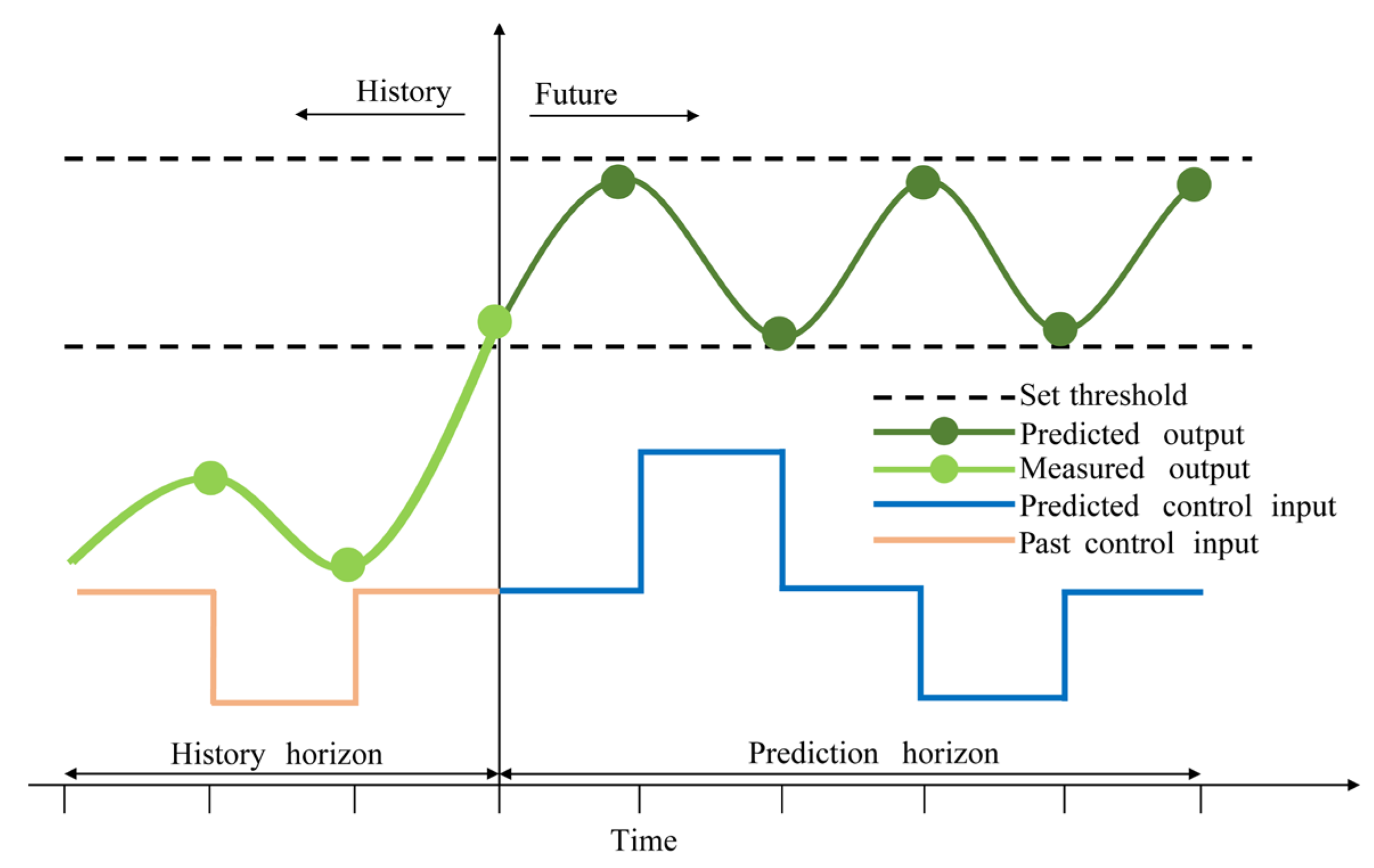
At each time step, MPC performs dynamic optimization within a finite time window, and the schematic of the MPC method is presented in Figure 2. By leveraging input data from the three most recent time instances, it predicts future indoor temperatures and employs an optimization algorithm to minimize the objective function. This process yields the optimal control action to maintain the indoor temperature within the predefined threshold range.

The predictive performance of MPC relies on dynamic modeling to generate control commands, so constructing an accurate predictive model is crucial. The mushroom room air conditioning system can be regarded as a nonlinear system with multiple inputs and a single output. Assume that the neural network prediction model of the system is as shown in Equation (12).

$$t(k+1)=f(t(k),d(k+1),u(k+1))$$

(12)

where $t$ is the indoor temperature, $f(\cdot )$ is a nonlinear function, $d$ is the outdoor temperature, $u$ is the control variable, i.e., the air conditioning runtime, and $k$ is the number of sampling periods.

2.4. Predictive Model

From Equation (12), the prediction model serves as the foundation for implementing the MPC method, and the GRU is suitable for time series prediction. The GRU is a type of recurrent neural network (RNN), similar to the LSTM network, and both are designed to address issues such as long-term memory dependence and gradient vanishing in backpropagation [28]. Compared with LSTM, the GRU merges the forget gate and the input gate into a single update gate and retains only the hidden state, thereby reducing the number of parameters and computational complexity [29]. This structural simplification results in shorter training durations and significantly enhances training efficiency. Through its gating mechanisms, the GRU dynamically selects and retains critical information while discarding irrelevant data at each time step, enabling more effective processing of extended temporal sequences. In practical applications, it is commonly integrated with attention mechanisms to further optimize performance.

Attention mechanism represents a pivotal technology in the field of deep learning, especially for processing long time-series data. Its core principle enables models to dynamically assign varying weights to different segments of the input, thereby focusing on the most critical information for the task [30]. By introducing the Attention mechanism, the model is enabled to capture key information changes more accurately. The GRU-Attention prediction model effectively captures complex nonlinear dependencies and further improves the accuracy of temperature prediction. The structure of the model is shown in Figure 3.

In this paper, GRU-Attention was employed as the prediction model for the MPC method, and the general steps were as follows:

(1)

Outdoor temperature, indoor temperature, and air conditioning runtime were normalized as input data and fed into the prediction model.

(2)

The normalized data were passed into the GRU, where a preliminary temperature prediction was generated.

(3)

The weights of the data features obtained from the GRU module were recalculated and reassigned through the Attention mechanism, thereby enhancing the focus on important information.

(4)

The processed data were fed into the fully connected layer to output the prediction results. After the prediction was completed, the data were inverse normalized, and the predicted values were compared with the actual values.

To enhance the predictive accuracy of the prediction model, the Optuna 1.4.0 optimization framework was selected to optimize the hyperparameters of the GRU-Attention prediction model. As an optimization framework based on an improved Bayesian optimization approach, Optuna demonstrates superior efficiency and convergence compared to traditional grid search and random search methods [31]. The default tree-structured parzen estimator (TPE) optimization algorithm [32] in the Optuna optimization framework enables hyperparameters to be automatically optimized to reduce fitting errors. This framework supports the dynamic construction of hyperparameter search spaces and efficiently performs pruning and search operations. By analyzing accumulated historical trial data, Optuna determines the next set of hyperparameter combinations to be evaluated, identifies potential high-performance hyperparameter regions, and conducts in-depth searches to obtain superior solutions. As new test results are generated, the framework continuously updates the search strategy and evaluates optimization effectiveness, thereby gradually enhancing the accuracy and reliability of the hyperparameter combinations and making them more suitable for real and complex environments. The core principle of Optuna is to model the hyperparameter space using a probabilistic model and to identify the optimal hyperparameter settings during model tuning to improve model performance. The Optuna hyperparameter optimization pseudocode is shown in Algorithm 1.

Algorithm 1: Pseudocode for hyperparameter optimization of GRU-Attention model using Optuna

Input: Training data x, Labels y, Number of trials T, Search space of the hyperparameter set H for the GRU-Attention model Output: Optimal hyperparameter combination H* for the GRU-Attention model after optimization 1 Define the objective function F(H), which computes the RMSE between actual and predicted temperatures 2 Select the hyperparameter set H to be optimized and define its search space 3 Create an Optuna study S for a single optimization task, specifying the objective function F(H) to be minimized, and use the TPE algorithm as the sampler 4 Run the optimization S·optimize(F, n_trials = …), where F is the objective function 5 The optimal hyperparameter set H* is the combination corresponding to the minimum objective function value after T trials 6 Apply the optimal hyperparameter combination H* to the predictive model

2.5. Rolling Optimization

The MPC is implemented as a rolling optimization, where at each sampling moment, a nonlinear optimization problem must be solved to enable the air conditioning system to execute the optimal control output. An objective function was established based on high temperature prediction accuracy and low energy consumption of the air conditioning system, as shown in Equation (13).

$$j(k)={\sigma }_1{\displaystyle \sum _{i=1}^{N_p}u{(k+i)}^2+}{\sigma }_2{\displaystyle \sum _{i=1}^{N_p}{\left[\max (T_{\min }-T_{pre}(k+i),0)+\max (T_{pre}(k+i)-T_{\max },0)\right]}^2}$$

(13)

where $N_p$ is the prediction time domain, $N_c$ is the control time domain ($N_p\ge N_c\ge 1$), ${\sigma }_1$, ${\sigma }_2$ are the weighting coefficients of each term in the objective function, $u$ is the air conditioning runtime, $k$ is the discrete-time index, $T_{pre}$ is the predicted temperature, and $T_{\max }$, $T_{\min }$ are the upper and lower limits of the temperature threshold.

In Equation (13), the first term on the right side represents the control energy consumption term. Minimizing this term reduces the operational duration of the air conditioning system. The second term represents the accuracy term. Minimization ensures that the predicted temperature remains within the predefined threshold.

The running interval of the air conditioner should not be excessively brief, as it leads to frequent system startups. This not only impairs equipment heat dissipation but also, more seriously, reduces the service life of the unit. Typically, the interval should be longer than 3 min. Considering these factors, to ensure safe operation, the start and stop of the air conditioner are treated as a constraint that must be satisfied and are not incorporated into the objective function. The shutdown duration of the air conditioner must satisfy one of the conditions given in Equations (14)–(16), while the running duration must satisfy Equation (17).

$$\left[u(k-1)=10\vee u(k-1)\le 7\right]\wedge \left[u(k+1)=0\right]$$

(14)

$$\left[u(k-1)=10\vee u(k-1)\le 7\right]\wedge \left[u(k)\le 7\vee u(k)=10\right]\wedge \left[u(k+1)>0\right]$$

(15)

$$\left[7<u(k-1)<10\right]\wedge \left[u(k)=0\right]$$

(16)

$$u(k)\ge 3$$

(17)

By iteratively substituting the inputs and outputs of the predictive model into the objective function to minimizing it, the optimal control sequence within a given time horizon is obtained. The first control variable of this sequence is applied as the control signal to the air conditioning system, and this process is repeated to realize rolling horizon optimization.

To address the aforementioned nonlinear optimization problem, reduce the computational cost associated with traditional iterative methods, and overcome the insufficient convergence accuracy of the COA, this paper proposed an ICOA to solve the objective function $j(k)$ and obtain the optimal control sequence. The optimization process of ICOA is divided into the following steps:

(1)

Initialization stage

In a multi-dimensional optimization problem, each crayfish represents a 1 × dim matrix, with each column corresponding to a solution to the problem. The ICOA is initialized based on a set of candidate solutions $x$ randomly generated between the upper and lower bounds. The ICOA initialization is shown in Equation (18), and the initial population position is calculated from Equation (19).

$$x=[x_1,x_2,\dots x_N]=\left[\begin{array}{ccccc}{x}_{1,1}& \dots & x_{1,j}& \dots & x_{1,dim}\\ ⋮& ⋮& ⋮& ⋮& ⋮\\ x_{i,1}& \dots & x_{i,j}& \dots & x_{i,dim}\\ ⋮& ⋮& ⋮& ⋮& ⋮\\ x_{N,1}& \dots & x_{N,j}& \dots & x_{N,dim}\end{array}\right]$$

(18)

$$x_{i,j}=l{b}_j+(u{b}_j-l{b}_j)\times rand$$

(19)

where $N$ is the population size, dim is the number of population dimensions, $x_{i,j}$ is the position of individual $i$ in dimension $j$, $l{b}_j$ is the lower bound of the $j$th dimension, $u{b}_j$ is the upper bound of the $j$th dimension, and $rand$ is a [0, 1] random number.

(2)

Define temperature and food intake

At different environmental temperatures, crayfish exhibit different behaviors, causing them to enter different stages. The temperature calculation formula is shown in Equation (20). When the temperature exceeds 30 °C, crayfish make heat avoidance behavior, when the temperature is suitable, crayfish will make foraging behavior. The food intake of crayfish is also affected by temperature, which ranges from 20 to 35 °C, with an optimal temperature of 25 °C. Therefore, the food intake of crayfish is approximately normally distributed $p$, calculated from Equation (21).

$$temp=rand\times 15+20$$

(20)

$$p=C_1\times \left({\displaystyle \frac{1}{\sqrt{2\times \pi }\times \sigma }}\right)\times \exp \left(-{\displaystyle \frac{{(temp-\mu )}^2}{2{\sigma }^2}}\right)$$

(21)

(3)

Summer resort stage

When the ambient temperature exceeds 30 °C, crayfish enter their caves to escape the heat, the definition of cave $x_{\mathrm{shade}}$ is shown in Equation (22).

$$x_{\mathrm{shade}}={\displaystyle \frac{x_G+x_L}{2}}$$

(22)

where $x_G$ is the optimal position obtained by iteration, $x_L$ is the optimal position of the current population.

Crayfish competition for caves is considered a stochastic event, and in COA, when $rand<0.5$ indicates that no competitive occurs, the crayfish enter the cave directly through Equation (23) to escape the heat.

$$x_{i,j}^{t+1}=x_{i,j}^t+C_2\times rand\times (x_{\mathrm{shade}}-x_{i,j}^t)$$

(23)

$$C_2=2-{\displaystyle \frac{t}{T}}$$

(24)

where $t$ is the current number of iterations, $C_2$ is the decreasing curve, calculated from Equation (24), and $T$ is the maximum number of iterations.

(4)

Competition stage

When the temperature exceeds 30 °C and $rand\ge 0.5$, it indicates that other crayfish are present in the cave, and the cave is competed for using Equation (25).

$$x_{i,j}^{t+1}=x_{i,j}^t-x_{z,j}^t+x_{\mathrm{shade}}$$

(25)

$$z=round\left[rand\times (N-1)\right]$$

(26)

where $z$ is a random individual of crayfish, calculated from Equation (26).

(5)

Foraging stage

When the temperature is at or below 30 °C, crayfish come out of their holes to forage for food, the position of the food is shown in Equation (27). When food is found, crayfish decide whether to shred it based on its size, and the food size is calculated from Equation (28).

$$x_{\mathrm{food}}=x_G$$

(27)

$$Q=C_3\times rand\times \left({\displaystyle \frac{fitnes{s}_i}{fitnes{s}_{\mathrm{food}}}}\right)$$

(28)

where $x_{\mathrm{food}}$ is the location of the food, $Q$ is the size of the food, $C_3$ is the food factor, which indicates the largest food and has a value of constant 3, $fitnes{s}_i$ is the fitness value of the $i$th crayfish, and $fitnes{s}_{\mathrm{food}}$ is the fitness value of the location of the food.

When $Q>{\displaystyle \frac{C_3+1}{2}}$, the food is too large and need to shred food before eating, as shown in Equation (29).

$$x_{\mathrm{food}}=\exp \left(-{\displaystyle \frac{1}{Q}}\right)\times x_{\mathrm{food}}$$

(29)

During the foraging stage, the step size for individual crayfish moving toward the globally optimal position is randomly dynamic and primarily determined by ambient temperature, which lacks adaptive regulation as the number of iterations increases. This limitation makes it difficult to perform refined searches in the later stages and causes oscillations near the optimum value. To enhance the convergence efficiency in the foraging stage and improve the precision of solutions in later phases, a time decay factor was introduced into the original crayfish foraging formula, as shown in Equation (30).

$$\alpha (t)={\alpha }_{initial}\times {\left({\displaystyle \frac{{\alpha }_{final}}{{\alpha }_{initial}}}\right)}^{{\displaystyle \frac{t}{T}}}$$

(30)

where ${\alpha }_{initial}$ represents the initial step size set to 1, maintaining the global search capability consistent with COA during the early stages, ${\alpha }_{final}$ denotes the final step size set to 0.01, ensuring sufficiently small step sizes in the later stages to achieve more refined local search and enhance convergence accuracy.

After food is shredded, crayfish feed by alternating their claws. To simulate this alternating feeding process, a method combining sine and cosine functions was employed. Furthermore, the amount of food obtained by the crayfish is also related to the feeding rate, as shown in Equation (31).

$$x_{i,j}^{t+1}=x_{i,j}^t+\alpha (t)\times x_{\mathrm{food}}^t\times p\times [\cos (2\times \pi \times \mathrm{rand})-\sin (2\times \pi \times \mathrm{rand})]$$

(31)

When $Q\le {\displaystyle \frac{C_3+1}{2}}$, crayfish will move directly toward food and consume it, as shown in Equation (32).

$$x_{i,j}^{t+1}=\alpha (t)\times [(x_{i,j}^t-x_{\mathrm{food}}^t)\times p+p\times \mathrm{rand}\times x_{i,j}^t]$$

(32)

The introduction of a time decay factor during the foraging stage gradually reduces the step size throughout iterations. In the early stage of iteration, a larger step size enhances the efficiency of global exploration, thereby preventing premature convergence to local optima and enabling the optimization process to approach the global optimum region more rapidly and effectively. In the later stage of iteration, a smaller step size improves the effectiveness of local fine search, enabling the algorithm to converge more stably and accurately near the optimal solution while avoiding oscillations caused by excessively large step sizes. This allows ICOA to approach the global optimum more reliably and precisely. The ICOA flowchart is illustrated in Figure 4.

2.6. Feedback Correction

In practical applications, there are uncertainties in the system, such as nonlinearity, time-varying characteristics, and external disturbances, which cause the gradual deterioration of the performance of the prediction model. MPC incorporates a feedback correction mechanism that updates the real-time measured state of the system at each rolling horizon moment, thereby correcting prediction errors, enhancing accuracy, and improving disturbance rejection and robustness. To mitigate the impact of deviations as much as possible, this paper implemented feedback compensation based on prediction error feedback.

After obtaining the actual temperature and predicted temperature at the $k+1$ moment, feedback control is performed using the error between the two. The prediction error is calculated using Equation (33).

$$T_{pre}(k+1)-T_r(k+1)=e_{mpc}(k+1)$$

(33)

where $T_{pre}$ is the actual temperature, $e_{mpc}$ is the error between the predicted temperature and the actual temperature.

This error is used to feedback and adjust the predicted temperature in the next prediction time domain. The corrected predicted temperature is calculated using Equation (34).

$${T^{\prime }}_{pre}(k+i)=T_{pre}(k+i)+h{e}_{mpc}(k+i)(i=2,3,\dots ,N)$$

(34)

where ${T^{\prime }}_{pre}$ is the corrected predicted temperature; $h$ is the feedback correction coefficient (with a value between 0~1).

The corrected predicted temperature is incorporated into a new round of rolling optimization, thereby forming a closed-loop control system and enhancing control reliability.

2.7. Assessment Indicators

To evaluate the effectiveness of the sensor optimization method based on the combination of PCA and information entropy, the Pearson correlation coefficient $\rho$ of the mean temperature series and the mean square error (MSE) of the temperature field reconstruction.

First, the average temperature sequence ${\overline{T}}_{full}[t]$ of all sensors was calculated by Equation (35), and the average temperature sequence ${\overline{T}}_{sel}[t]$ of the selected sensors was calculated by Equation (36). Then, the Pearson correlation coefficient $\rho$ of these two average temperature sequences was calculated by Equation (37). This Pearson correlation coefficient is used to measure the degree of linear correlation between the mean temperature series calculated from the selected sensors and that calculated from all sensors. The value closer to 1 indicates a higher degree of similarity between the two.

$${\overline{T}}_{full}[t]={\displaystyle \frac{1}{\mathrm{n}}}{\displaystyle \sum _{i\in n}{T}_i}$$

(35)

$${\overline{T}}_{sel}[t]={\displaystyle \frac{1}{s}}{\displaystyle \sum _{j\in s}{T}_j}$$

(36)

$$\rho ={\displaystyle \frac{{\displaystyle \sum _{t=1}^T(T_{\mathrm{full}}[t]-{\overline{T}}_{\mathrm{full}}[t])}(T_{\mathrm{sel}}[t]-{\overline{T}}_{\mathrm{sel}}[t])}{\sqrt{{\displaystyle \sum _{t=1}^T{(T_{\mathrm{full}}[t]-{\overline{T}}_{\mathrm{full}}[t])}^2}}\cdot \sqrt{{\displaystyle \sum _{t=1}^T{(T_{\mathrm{sel}}[t]-{\overline{T}}_{\mathrm{sel}}[t])}^2}}}}$$

(37)

where $s$ is the index of the selected sensor.

The average temperature sequence of the selected sensors was used to represent the reconstruction method of the entire temperature field. Equation (38) was used to calculate the MSE between the average temperature sequence of all sensors and the reconstructed temperature sequence, in order to measure the error when the selected sensors were used to approximate the mean of the entire temperature field. The smaller the MSE, the better the reconstruction effect.

$$MSE={\displaystyle \frac{1}{T}}{\displaystyle \sum _{t=1}^T{\left({\overline{T}}_{full}[t]-{\overline{T}}_{sel}[t]\right)}^2}$$

(38)

To evaluate the performance of the prediction model, this study used root mean square error (RMSE), coefficient of determination (R²), and mean absolute percentage error (MAPE) as assessment indicators.

3. Results

3.1. Sensor Number Selection and Results Analysis

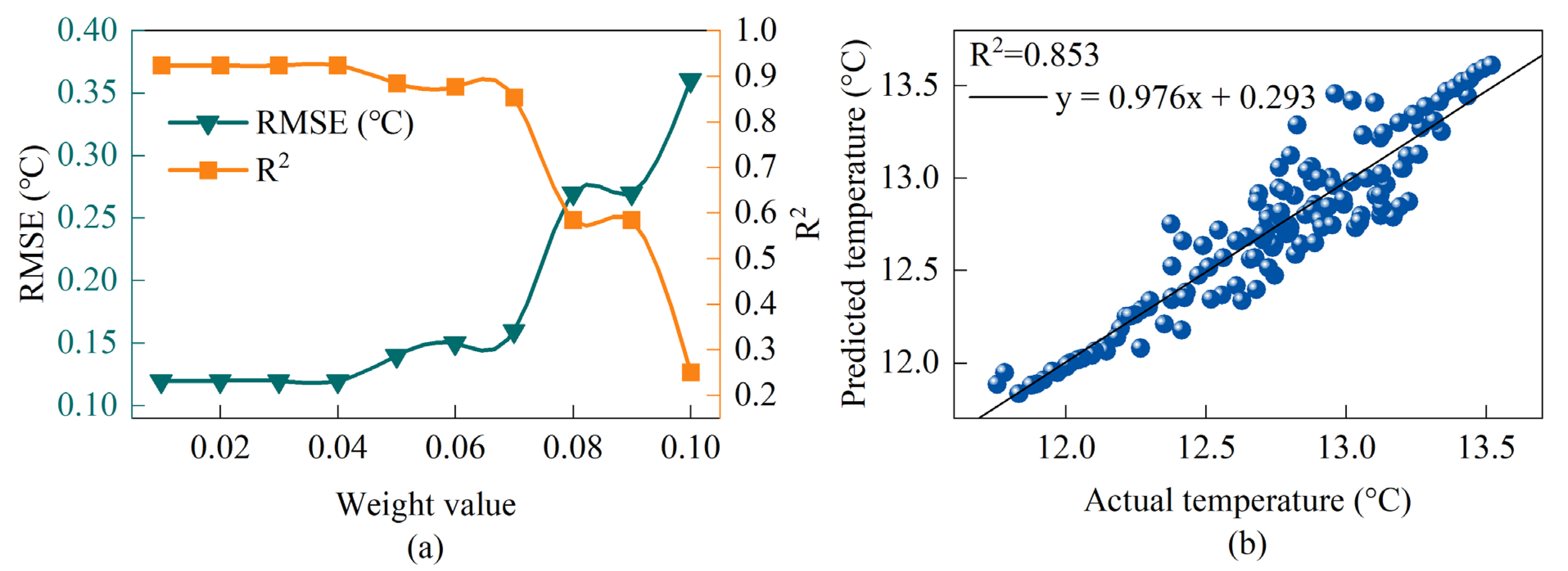
As shown in Equation (11), the weight $\alpha$ corresponding to the number of sensors exerts a significant influence on sensor selection, thereby affecting the training process of the prediction model. To investigate the impact of weight on model accuracy, this paper established a series of distinct weight values and employed the discrete binary particle swarm optimization (BPSO) algorithm [33] to solve the objective function (11). The resulting sensor configurations under varying weights $\alpha$ are shown in

Table 2. Selected sensors and corresponding metrics under different weights.

$\mathit{\alpha }$ Value	Selected Sensor Number	Variance Contribution Rate	Information Capture Rate
0.01~0.04	all sensors	100%	100%
0.05	1, 3, 4, 5, 6, 7, 8, 9, 10, 12, 15, 16	82.71%	98.87%
0.06	4, 6, 7, 12, 15	45.71%	96.46%
0.07	7, 12, 15	33.56%	95.77%
0.08~0.09	7, 12	26.43%	87.63%
0.1	12	7.13%	64.05%

.

As shown in Table 2, the number of selected sensors gradually decreased as the weight $\alpha$ of sensor quantity increased, while both the variance contribution rate and information capture rate exhibited a corresponding decline. To determine the optimal sensor count, models with different sensor counts were compared. Data from 15 January to 24 January were used as the training set, and the average temperature calculated from all sensors on 25 January was predicted. The prediction results are shown in Figure 5.

As shown in Figure 5, prediction accuracy gradually decreased as the sensor weight increased. The model achieved optimal performance when the weight ranged between 0.01 and 0.04, with an RMSE of 0.12 °C and an R² of 0.923. When the weight progressively increased to 0.07, the RMSE rose to 0.16 °C and R² decreased to 0.853, the model performance showed only minor degradation, but the number of sensors was reduced by 81.25%. For weights of 0.08 to 0.09, RMSE increased to 0.27 °C and R² fell to 0.584. At a weight of 0.1, RMSE reached 0.36 °C and R² dropped to 0.251, indicating that the model fails to accurately predict temperature. In summary, this paper ultimately selected the sensor configuration corresponding to a weight of 0.07, comprising sensors numbered 7, 12, and 15. This selection not only reduced equipment procurement and maintenance costs but also decreased model complexity and computational expenses. Evaluation of the selected sensors using Equations (37) and (38) yielded a Pearson correlation coefficient of 0.977 and an MSE of 0.04 °C. The results demonstrated that the selected sensors effectively represented the variations in the entire temperature field.

3.2. Predictive Model Analysis

To accurately predict indoor temperatures of mushroom room, the average temperature from selected sensors, the mean outdoor temperature from four external sensors, and the operational duration of air conditioning units measured by current sensors were utilized as inputs for the prediction models. Four distinct predictive models were employed: convolutional neural network (CNN), CNN-Attention, GRU, and GRU-Attention. The optimal model was selected through comprehensive evaluation of performance metrics. This paper employed the Optuna optimization framework to tune the hyperparameters of four prediction models. The types of hyperparameters, their search spaces, and the optimized values are detailed in

Table 3. Hyperparameter optimization for predictive models.

Predictive Model	Hyperparameters Name	Search Space	Best Hyperparameters
CNN	Number of convolutional layers	[1, 2, 3]	1
	Number of filters 1	[16, 32, 64, 128]	64
	FC units 2	[16, 32, 64, 128]	128
	Learning rate	[1 × 10−4~1 × 10−2]	0.00390567294
	Batch size	[8, 16, 32, 64]	8
	Epochs	[30~100]	57
CNN-Attention	Number of convolutional layers	[1, 2, 3]	1
	Number of filters 1	[16, 32, 64, 128]	64
	Attention layer dimension	[16, 32, 64, 128]	128
	FC units 2	[16, 32, 64, 128]	16
	Learning rate	[1 × 10−4~1 × 10−2]	0.0028632374
	Batch size	[8, 16, 32, 64]	8
	Epochs	[30~100]	77
GRU	Number of GRUs	[16, 32, 64, 128]	16
	FC units 2	[16, 32, 64, 128]	64
	Learning rate	[1 × 10−4~1 × 10−2]	0.0045723438
	Batch size	[8, 16, 32, 64]	8
	Epochs	[30~100]	56
GRU-Attention	Number of GRU layer units	[16, 32, 64, 128]	64
	Attention layer dimension	[16, 32, 64, 128]	32
	FC units 2	[16, 32, 64, 128]	32
	Learning rate	[1 × 10−4~1 × 10−2]	0.0016217518
	Batch size	[8, 16, 32, 64]	8
	Epochs	[30~100]	72

¹ Number of filters: Number of convolutional filters per convolutional layer. ² FC units: Number of units in each fully connected layer.

. In the tests, the dataset was divided into 80% for training and 20% for testing. The training set was used for parameter learning and optimization, while the test set was used to evaluate the generalization capability and prediction accuracy of the models on unseen data. The performance evaluation metrics for each model are presented in

Table 4. Comparison of performance of different predictive models.

Predictive Model	RMSE (°C)	R2	MAPE (%)	Computation Time (s)
CNN	0.20	0.899	1.29	37
CNN-Attention	0.19	0.909	1.17	76
GRU	0.21	0.884	1.22	35
GRU-Attention	0.17	0.926	0.99	42

.

In terms of error accuracy, the GRU-Attention model achieved an RMSE of 0.17 °C on the test set, which was 15.0%, 10.5%, and 19.0% lower than those of CNN, CNN-Attention, and GRU models, respectively, significantly reduced the absolute deviation between predicted and actual values. Regarding fitting capability, its R² reached 0.926, which represented an improvement of 1~5% over the other models and indicated stronger interpretability of the inherent patterns in time-series data. In terms of percentage error, the MAPE of GRU-Attention was 0.99%, reflected reductions of 23.3%, 15.4%, and 18.9% compared to CNN, CNN-Attention, and GRU models, respectively, which highlighted its superior accuracy in relative error control. Although the runtime of GRU-Attention was not the shortest, the control cycle was considerably longer than the runtime of the prediction model. Given its superior performance in RMSE, R², and MAPE compared to other models, GRU-Attention was selected as the predictive model in this paper.

3.3. Optimization Algorithm Analysis

To identify suitable optimization algorithm for the optimized control of mushroom room air conditioning system, this paper compared the performance of genetic algorithm (GA), simulated annealing (SA), particle swarm optimization (PSO), sparrow search algorithm (SSA), and COA with the proposed ICOA optimization algorithm. Under identical population sizes, they were applied to control indoor temperature with the two weight coefficients in the objective function set to 1 and 1000, respectively. The comparison results are shown in

Table 5. Performance comparison of different optimization algorithms.

Optimization Algorithm	Population Size	Fitness Value j(k)
GA	30	107.66
SA		120.51
PSO	30	74.36
SSA	30	62.45
COA	30	49.36
ICOA	30	24.19

.

As shown in Table 5, significant differences existed in the fitness values among the various optimization algorithms. Under identical population sizes, GA, SA, PSO, and SSA exhibited relatively high fitness values, indicating comparatively inferior optimization performance. The fitness value of COA was 49.36, showing improvement over the four preceding algorithms. ICOA achieves the best performance, reducing the fitness value by approximately 51% compared to COA. This result indicated that the introduction of a time decay factor significantly enhanced convergence accuracy. Among the multiple optimization algorithms evaluated, ICOA exhibited superior optimization effect.

To further validate the stability of ICOA solutions, ten independent trials were conducted under identical conditions, with the fitness values recorded for each run. The results are shown in

Table 6. Statistical results of ICOA fitness values.

No.	Fitness Value j(k)	No.	Fitness Value j(k)
1	24.19	6	26.05
2	24.35	7	23.52
3	27.42	8	23.72
4	22.50	9	22.14
5	24.62	10	23.72

.

As shown in Table 6, the fitness values of ICOA ranged from 22.14 to 27.42, with an overall limited fluctuation range. The optimal fitness value was 22.14, the worst fitness value was 27.42, the average was 24.22, and the standard deviation was merely 1.56. These results indicated that ICOA exhibited favorable solution stability under repeated execution conditions. In conclusion, this paper selected ICOA as the optimization solver for MPC.

3.4. Predictive Time Step Analysis

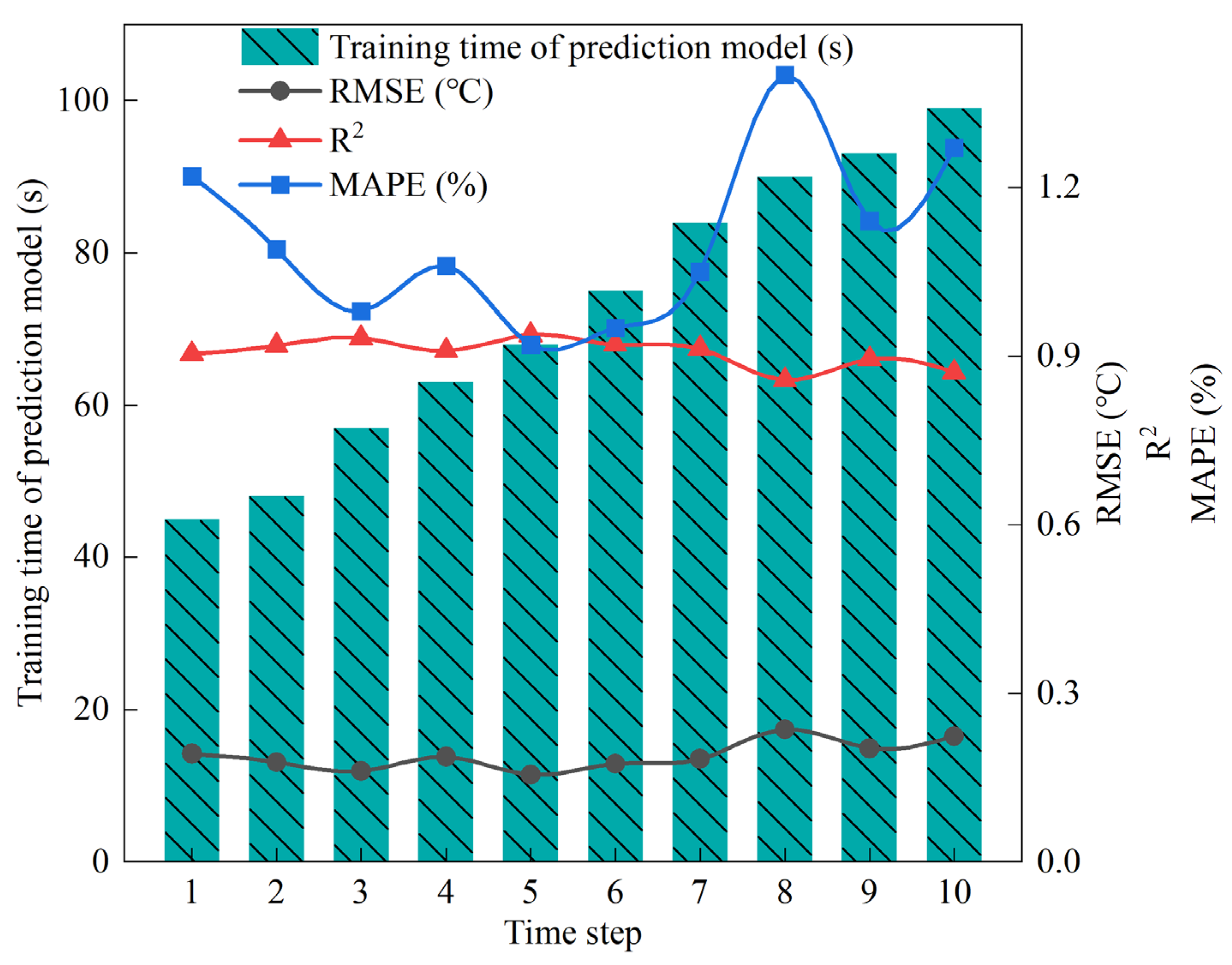
The selection of time step size significantly influences both the prediction model accuracy and training duration, so it is necessary to choose the appropriate prediction time step, and select the appropriate parameters from the time steps of 1 to 10, representing a historical time period of 10 to 100 min. The experimental results are shown in Figure 6, the prediction model training time was proportional to the prediction time step, when the prediction time step was 5, the prediction accuracy was the highest, but the prediction time step was too long, resulting in the current moment air conditioning runtime having no significant impact on the temperature of the next moment. This caused all terms in Equation (13) to be optimized to 0, which contradicted actual conditions. It was experimentally verified that the prediction time step was chosen to be 3, meaning that the historical 30 min time period data predicted the average indoor temperature for the next 10 min time period.

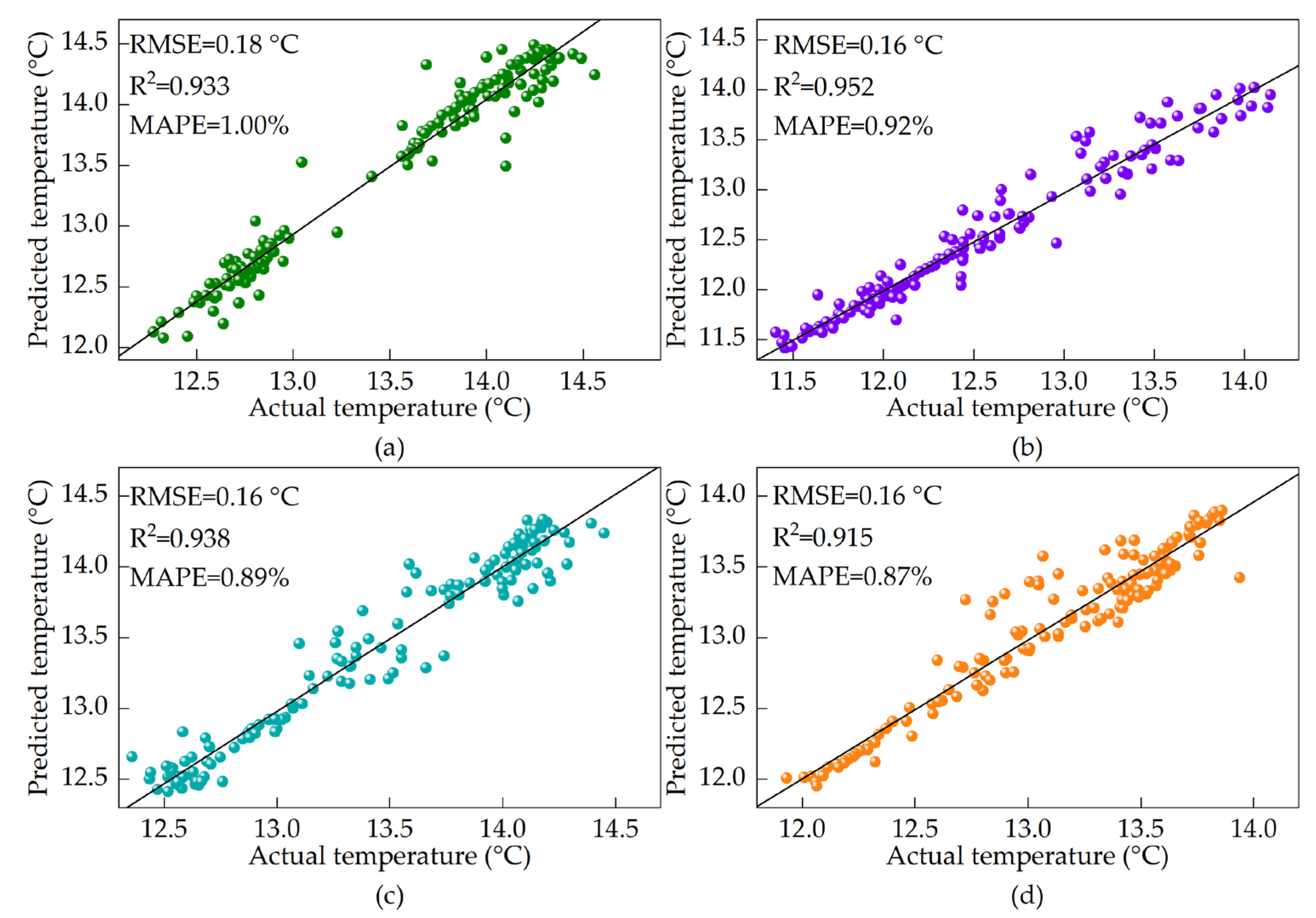
To further validate the appropriateness of the time step selection, data from 22 January to 25 January were utilized for prediction. The fit between predicted and measured temperatures was shown in Figure 7, with a maximum error of 0.64 °C, a mean error of 0.12 °C, a maximum RMSE of 0.18 °C, a minimum R² of 0.915, and a maximum MAPE of 1.00%. The results indicated that under a time step of 3, the forecast results maintained good consistency with the actual data.

3.5. Objective Function Weight Analysis

The objective function in the MPC is shown in Equation (13), and determining the weights is the key to the solution. Two weight coefficients need to be set in Equation (13), weight coefficient σ₁ for the energy consumption term and weight coefficient σ₂ for the accuracy term. To ensure both terms were within the same order of magnitude and to prioritize maintaining mushrooms within a suitable temperature range for growth, the weighting coefficient for the energy consumption term was empirically set to 1, while that for the accuracy term was set to 1000 for preliminary analysis. Building on this, a strategy of fixed accuracy weighting with gradual adjustments to the energy consumption weighting was adopted. Comparative experiments were conducted on system performance under various weighting combinations, with the results illustrated in Figure 8. The MPC strategy set the temperature threshold range to 13.5~15.5 °C. The energy consumption weight was sequentially set to 0.01, 0.1, 1, 10, and 100 to analyze how these adjustments affected temperature control stability, environmental suitability, and energy savings, thereby identifying the optimal weight combination.

As shown in Figure 8, under the condition of a fixed accuracy term weight of 1000, the air conditioning runtime gradually shortened and system energy consumption de-creased as the energy consumption term weight increased. When the energy consumption term weight increased from 0.01 to 0.1, the air conditioning runtime decreased from 367 min to 364 min, demonstrating negligible energy savings. This occurred because the energy consumption term exerted minimal influence in the objective function, with the optimization process entirely dominated by the accuracy term. When the energy consumption weight increased to 1, the air conditioning runtime shortened to 321 min, achieving significant energy savings while maintaining temperature control precision. However, when the energy consumption weight rose to 10 or higher, the temperature control performance of the MPC method deteriorated markedly, with indoor temperatures falling below the lower threshold. This indicated the influence of the accuracy term in the objective function was excessively weakened, effectively ignored, leading to severe deviations from the optimal temperature range. Balancing energy efficiency and temperature control precision, a weight of 1 for the energy consumption term and 1000 for the accuracy term in the objective function was selected. This configuration ensured mushroom growth within the optimal temperature range while reducing energy consumption.

3.6. Assessment of MPC Performance

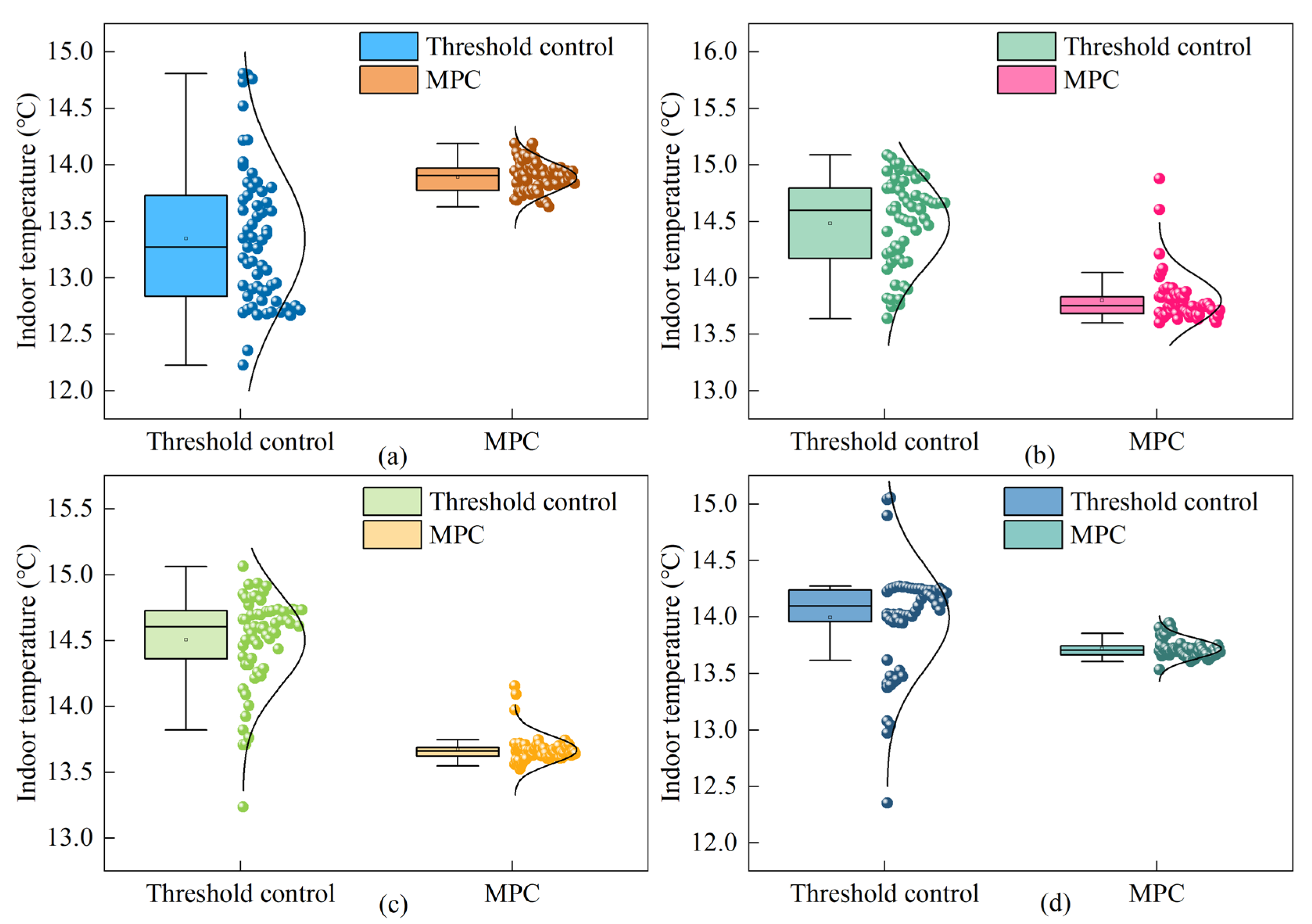
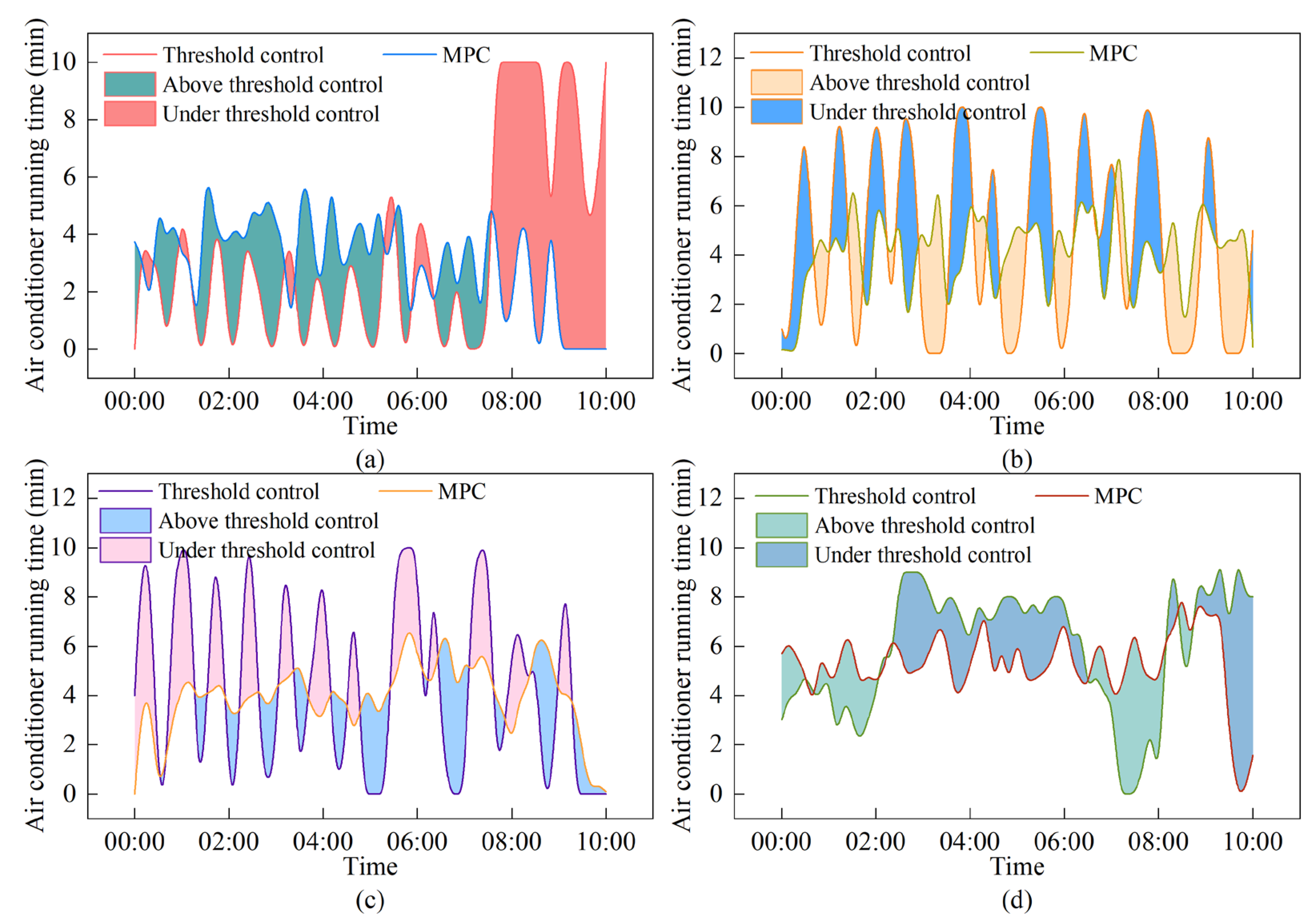
In order to validate the control effectiveness of the constructed MPC method based on the predictive model, a four-day experimental period from 16 January to 19 January was selected, with 10 h of testing conducted each day. The temperature range of the MPC method was set between 13.5 °C and 15.5 °C. This was compared with a threshold control method, which employed the same temperature range. Under threshold control, heating was commenced when temperatures detected by sensors fell below 13.5 °C and ceased when temperatures reached 15.5 °C. Figure 9 illustrates the mushroom room temperature comparison under both control modes, while Figure 10 shows the air conditioner operating duration.

Figure 9 illustrated the indoor temperature fluctuation ranges in the mushroom room controlled by the threshold control method and the MPC method. The threshold control method maintained indoor temperature within ranges of 12.22~14.81 °C, 13.64~15.09 °C, 13.23~15.06 °C, and 12.35~15.05 °C, respectively. In contrast, the MPC method regulated temperatures within ranges of 13.63~14.19 °C, 13.60~14.87 °C, 13.52~14.15 °C, and 13.53~13.95 °C, respectively. As a result, the mushroom room temperature was observed to fluctuate significantly under threshold control, with 20.5% of temperature readings falling below the lower threshold limit. This occurs because threshold control often exhibited delayed response, initiating heating only after temperature dropped below the lower limit. In contrast, the MPC method avoided excursions beyond the predefined temperature range, demonstrating greater stability in controlling the indoor environment, with narrower overall temperature variations and superior control performance. Figure 10 presented the running time of the air conditioner under two control methods. The running times for the threshold control method were 211 min, 276 min, 271 min, and 358 min, respectively, while those for the MPC method were 186 min, 247 min, 238 min, and 321 min, corresponding to energy consumption reductions of 11.8%, 10.5%, 12.2%, and 10.3%, respectively. By predicting future states, the MPC method enabled preemptive heating before temperature decline, preventing overcompensation and thereby reducing total heating duration. Thus, the proposed MPC approach achieved energy savings while maintaining control accuracy.

4. Discussion

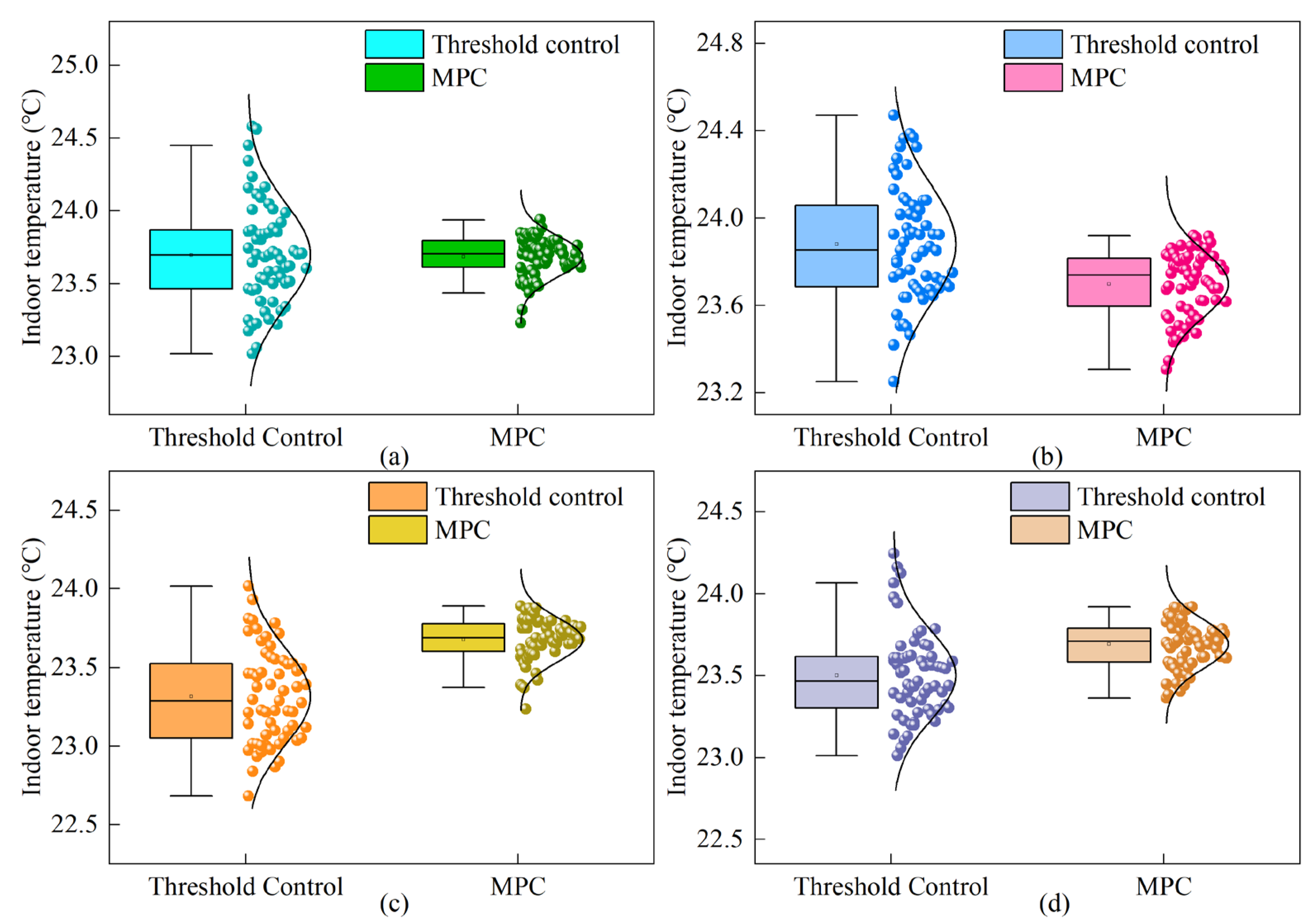
Based on the experimental verification conducted in winter, this study further extended the model predictive control method to summer environments for verification, aiming to assess its adaptability and energy-saving potential across different seasons. Given the persistent high temperatures in the external environment during summer, if the same set points as in winter were maintained mechanically, it would cause the refrigeration system to operate under high load for a long time to counteract the large temperature difference between inside and outside, resulting in significant energy consumption. To achieve a balance between economic benefits and cultivation benefits, we proposed a seasonal dynamic set-point strategy. We maintained optimal humidity levels of 85~95% in the mushroom cultivation room while raising the temperature control range to 22~24 °C. This configuration addressed engineering requirements by minimizing indoor-outdoor temperature differentials to reduce baseline cooling loads, while ensuring the Pleurotus citrinopileatus remained within their optimal temperature range. Moderately elevated temperatures also promoted mycelial metabolism, thereby shortening the production cycle. We selected the data from 18th June to 21st June, spanning 4 days, and conducted the experiment for 10 h each day. The MPC method was compared with the traditional threshold control method within the same temperature range.

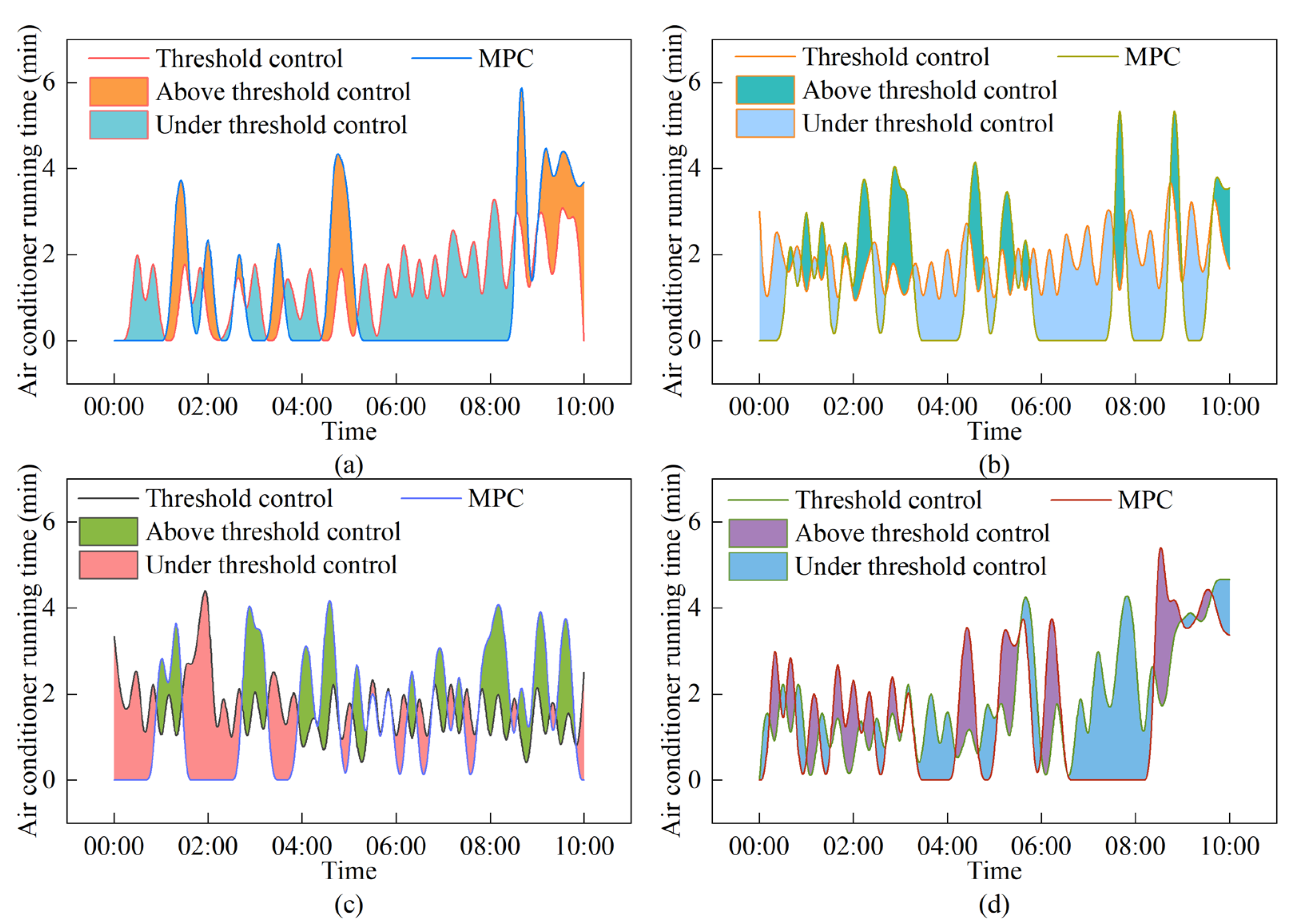
The indoor temperature changes under the two control methods are shown in Figure 11. The threshold control exhibited obvious temperature fluctuations, with some periods experiencing temperatures exceeding the set threshold. In contrast, under the MPC, the indoor temperature remained stable within the range of 22.5~23.8 °C, without any temperature overshoot phenomenon. The operating durations of the air conditioning refrigeration system under the two control methods are shown in Figure 12. Under MPC, the cumulative operating durations were 89 min, 110 min, 100 min, and 128 min, respectively, representing reductions of 11.0%, 16.7%, 13.0%, and 11.1% compared to the threshold control method’s durations of 100 min, 132 min, 115 min, and 144 min. This remarkable energy-saving effect stems from MPC’s ability to anticipate environmental changes and perform multi-variable cooperative optimization. This enables it to proactively respond to external conditions, smoothly regulate equipment operation, and prevent unnecessary energy waste. Experimental results conclusively demonstrate that the MPC strategy proposed in this study not only performs effectively in winter environments but also maintains stable environmental control performance under summer conditions while achieving significant energy savings. It exhibits excellent cross-seasonal adaptability, providing a reliable technical solution for the intelligent environmental management in edible mushroom production.

The MPC method proposed in this study can also be applied to the cultivation environments of other edible mushrooms. For example, compared to Pleurotus citrinopileatus, Hypsizygus marmoreus requires a similar humidity range of 85~95% for growth but is extremely sensitive to temperature, demanding strict control within the narrow range of 13~16 °C. Leveraging the precise control capabilities of the MPC method, the cultivation environment temperature can be stably maintained within the 13~16 °C range. This ensures normal growth of Hypsizygus marmoreus while further optimizing energy utilization. The model proposed in this study is applicable to mushroom growing control rooms that are equipped with air conditioners or other control devices. Therefore, the next step will focus on cross-scenario field verification, including typical scenarios such as ordinary plastic greenhouses, to evaluate the feasibility and benefits of the method in practical promotion.

5. Conclusions

Addressing the issue of sensor selection in mushroom room, this study proposed a combined approach of PCA and information entropy to optimize sensor configuration. The original set of 16 sensors was reduced to 3, achieving an 81.25% reduction in sensor count, which significantly decreased model complexity and computational costs. Using the average temperature series derived from all 16 sensors as a benchmark, the reconstructed temperature series from the selected three sensors were evaluated. The Pearson correlation coefficient between the two average temperature series was calculated as 0.977, with a MSE of 0.04 °C for the temperature field reconstruction. The evaluation results indicated that the selected sensors effectively represented the main variations in the indoor temperature field.

For prediction, a GRU-Attention neural network model was employed, with its hyperparameters optimized through the Optuna framework. During a 4-day temperature prediction period, the maximum error was 0.64 °C, the average error was 0.12 °C, the maximum RMSE was 0.18 °C, the minimum R² was 0.915, and the maximum MAPE was 1.00%. The results indicated that the proposed prediction model achieved high predictive accuracy and stability.

For control optimization, this paper proposed an ICOA based on the original COA framework. Compared to the primitive COA, ICOA achieved an approximately 51% reduction in fitness value, demonstrating superior convergence accuracy. Building upon this foundation, the ICOA was applied to optimize the MPC methodology. With objectives centered on achieving high precision and low energy consumption, the developed MPC model demonstrated exceptional temperature control performance while realizing an average energy savings of 11.2%. This approach provided significant energy efficiency benefits and smoother temperature regulation.

References

1. Sganzerla, W.G.; Todorov, S.D.; da Silva, A.P. Research Trends in the Study of Edible Mushrooms: Nutritional Properties and Health Benefits. Int. J. Med. Mushrooms 2022, 24, 1–18. [Google Scholar] [CrossRef]
2. Zhang, Y.; Wang, D.; Chen, Y.; Liu, T.; Zhang, S.; Fan, H.; Liu, H.; Li, Y. Healthy Function and High Valued Utilization of Edible Fungi. Food Sci. Hum. Wellness 2021, 10, 408–420. [Google Scholar] [CrossRef]
3. Liu, J.; Sun, J.; He, R.; Xia, J.; He, P. The situation of counterfeited and mislabeled commercialized edible mushrooms in China and the development of possible controls. Foods 2024, 13, 3097. [Google Scholar] [CrossRef]
4. Ali, B.M.; Akkaş, M. The green cooling factor: Eco-innovative heating, ventilation, and air conditioning solutions in building design. Appl. Sci. 2023, 14, 195. [Google Scholar] [CrossRef]
5. Adesanya, M.A.; Obasekore, H.; Rabiu, A.; Na, M.H.; Ogunlowo, Q.O.; Akpenpuun, T.D.; Kim, M.H.; Kim, H.T.; Kang, B.Y.; Lee, H.W. Deep reinforcement learning for PID parameter tuning in greenhouse HVAC system energy Optimization: A TRNSYS-Python cosimulation approach. Expert Syst. Appl. 2024, 252, 124126. [Google Scholar] [CrossRef]
6. Killian, M.; Kozek, M. Ten questions concerning model predictive control for energy efficient buildings. Build. Environ. 2016, 105, 403–412. [Google Scholar] [CrossRef]
7. Zhuang, J.; Chen, Y.; Chen, X. A new simplified modeling method for model predictive control in a medium-sized commercial building: A case study. Build. Environ. 2018, 127, 1–12. [Google Scholar] [CrossRef]
8. Salem, F.M.; Mosaad, M.I.; Awadallah, M.A. A comparative study of MPC and optimised PID control. Int. J. Ind. Electron. Drives 2015, 2, 242–250. [Google Scholar] [CrossRef]
9. Wang, M.; Zheng, W.; Zhao, C.; Zhang, X.; Kong, X.; Shan, F.; Zhao, Q. Energy-saving control method for factory mushroom room air conditioning based on MPC. Energies 2023, 16, 7623. [Google Scholar] [CrossRef]
10. Wang, D.; Chen, Y.; Wang, W.; Gao, C.; Wang, Z. Field test of Model Predictive Control in residential buildings for utility cost savings. Energy Build. 2023, 288, 113026. [Google Scholar] [CrossRef]
11. Jeon, B.K.; Kim, E.J. LSTM-Based Model Predictive Control for Optimal Temperature Set-Point Planning. Sustainability 2021, 13, 894. [Google Scholar] [CrossRef]
12. Yao, Y.; Shekhar, D.K. State of the art review on model predictive control (MPC) in Heating Ventilation and Air-conditioning (HVAC) field. Build. Environ. 2021, 200, 107952. [Google Scholar] [CrossRef]
13. Wang, H.; Bo, S.; Zhu, C.; Hua, P.; Xie, Z.; Xu, C.; Wang, T.; Li, X.; Wang, H.; Lahdelma, R. A zoned group control of indoor temperature based on MPC for a space heating building. Energy Convers. Manag. 2023, 290, 117196. [Google Scholar] [CrossRef]
14. Drgoňa, J.; Arroyo, J.; Figueroa, I.C.; Blum, D.; Helsen, L. All you need to know about model predictive control for buildings. Annu. Rev. Control 2020, 50, 190–232. [Google Scholar] [CrossRef]
15. Afroz, Z.; Shafiullah, G.; Urmee, T.; Higgins, G. Modeling techniques used in building HVAC control systems: A review. Renew. Sustain. Energy Rev. 2018, 83, 64–84. [Google Scholar] [CrossRef]
16. Kumar, P.; Rawlings, J.B.; Wenzel, M.J.; Risbeck, M.J. Grey-box model and neural network disturbance predictor identification for economic MPC in building energy systems. Energy Build. 2023, 286, 112936. [Google Scholar] [CrossRef]
17. Tol, H.İ.; Madessa, H.B. Development of a white-box dynamic building thermal model integrated with a heating system. J. Build. Eng. 2023, 68, 106038. [Google Scholar] [CrossRef]
18. Hu, Y.; Qin, L.; Li, S.; Li, X.; Zhou, R.; Li, Y.; Sheng, W. Adaptive corrected parameters algorithm applied in cooling load prediction based on black-box model: A case study for subway station. Energy Build. 2023, 297, 113429. [Google Scholar] [CrossRef]
19. Zhang, L.; Jin, G.; Liu, T.; Zhang, R. Generalized hierarchical expected improvement method based on black-box functions of adaptive search strategy. Appl. Math. Model. 2022, 106, 30–44. [Google Scholar] [CrossRef]
20. Wang, M.; Kong, X.; Shan, F.; Zheng, W.; Ren, P.; Wang, J.; Chen, C.; Zhang, X.; Zhao, C. Temperature Prediction of Mushrooms Based on a Data—Physics Hybrid Approach. Agriculture 2024, 14, 145. [Google Scholar] [CrossRef]
21. Afram, A.; Janabi-Sharifi, F. Review of modeling methods for HVAC systems. Appl. Therm. Eng. 2014, 67, 507–519. [Google Scholar] [CrossRef]
22. Mtibaa, F.; Nguyen, K.K.; Azam, M.; Papachristou, A.; Venne, J.S.; Cheriet, M. LSTM-based indoor air temperature prediction framework for HVAC systems in smart buildings. Neural Comput. Appl. 2020, 32, 17569–17585. [Google Scholar] [CrossRef]
23. Mtibaa, F.; Nguyen, K.K.; Dermardiros, V.; Cheriet, M. Context-aware model predictive control framework for multi-zone buildings. J. Build. Eng. 2021, 42, 102340. [Google Scholar] [CrossRef]
24. Zhang, J.; Poon, K.H.; Kwok, H.H.; Hou, F.; Cheng, J.C. Predictive control of HVAC by multiple output GRU-CFD integration approach to manage multiple IAQ for commercial heritage building preservation. Build. Environ. 2023, 245, 110802. [Google Scholar] [CrossRef]
25. Fujimori, K.; Goto, Y.; Liu, Y.; Taniguchi, M. Sparse principal component analysis for high-dimensional stationary time series. Scand. J. Stat. 2023, 50, 1953–1983. [Google Scholar] [CrossRef]
26. Merrikh-Bayat, F. The runner-root algorithm: A metaheuristic for solving unimodal and multimodal optimization problems inspired by runners and roots of plants in nature. Appl. Soft Comput. 2015, 33, 292–303. [Google Scholar] [CrossRef]
27. Jia, H.; Rao, H.; Wen, C.; Mirjalili, S. Crayfish optimization algorithm. Artif. Intell. Rev. 2023, 56 (Suppl. S2), 1919–1979. [Google Scholar] [CrossRef]
28. Chen, J.; Xu, G.; Zhou, Z. Data-driven learning-based Model Predictive Control for energy-intensive systems. Adv. Eng. Inform. 2023, 58, 102208. [Google Scholar] [CrossRef]
29. Zarzycki, K.; Ławryńczuk, M. Advanced predictive control for GRU and LSTM networks. Inf. Sci. 2022, 616, 229–254. [Google Scholar] [CrossRef]
30. Li, F.; Meng, X.; Zhu, K.; Yan, J.; Liu, L.; Liu, P. Research on Ginger Price Prediction Model Based on Deep Learning. Agriculture 2025, 15, 596. [Google Scholar] [CrossRef]
31. Li, Y.; Cao, Y.; Yang, J.; Wu, M.; Yang, A.; Li, J. Optuna-DFNN: An Optuna framework driven deep fuzzy neural network for predicting sintering performance in big data. Alex. Eng. J. 2024, 97, 100–113. [Google Scholar] [CrossRef]
32. Yu, J.; Zhao, Y.; Pan, R.; Zhou, X.; Wei, Z. Prediction of the critical temperature of superconductors based on two-layer feature selection and the optuna-stacking ensemble learning model. ACS Omega 2023, 8, 3078–3090. [Google Scholar] [CrossRef]
33. Beheshti, Z.; Shamsuddin, S.M.; Hasan, S. Memetic binary particle swarm optimization for discrete optimization problems. Inform. Sci. 2015, 299, 58–84. [Google Scholar] [CrossRef]
Figure 1. Schematic diagram of sensor installation and mushroom room structure: (a) Side view of mushroom room. (b) Front view of mushroom room.
Energies 18 05550 g001
Figure 2. Schematic of model predictive control (MPC).
Energies 18 05550 g002
Figure 3. Predictive model structure.
Energies 18 05550 g003
Figure 4. The flowchart of improved crayfish optimization algorithm (ICOA).
Energies 18 05550 g004
Figure 5. Prediction accuracy at different weights: (a) Comparison of prediction accuracy under different weights. (b) Prediction accuracy at a weight of 0.07.
Energies 18 05550 g005
Figure 6. Comparison of accuracy for different prediction time steps.
Energies 18 05550 g006
Figure 7. Prediction performance of the model: (a) 22 January; (b) 23 January; (c) 24 January; (d) 25 January.
Energies 18 05550 g007
Figure 8. Impact of different weights on system performance: (a) The impact of different weights on air conditioner operating time. (b) The impact of different weights on indoor temperature.
Energies 18 05550 g008
Figure 9. Indoor temperature under threshold control method and MPC method: (a) 22 January; (b) 23 January; (c) 24 January; (d) 25 January.
Energies 18 05550 g009
Figure 10. Air conditioning running time under threshold control method and MPC method: (a) 22 January; (b) 23 January; (c) 24 January; (d) 25 January.
Energies 18 05550 g010
Figure 11. Indoor temperature under threshold control method and MPC method: (a) 18 June; (b) 19 June; (c) 20 June; (d) 21 June.
Energies 18 05550 g011
Figure 12. Air conditioning running time under threshold control method and MPC method: (a) 18 June; (b) 19 June; (c) 20 June; (d) 21 June.
Energies 18 05550 g012