Article

Beyond R2: The Role of Polynomial Degree in Modeling External Temperature and Its Impact on Heat-Pump Energy Demand

by
Maciej Masiukiewicz
1,*,
Giedrė Streckienė
2 and
Arkadiusz Gużda
3
1
Department of Process and Environmental Engineering, Faculty of Mechanical Engineering, Opole University of Technology, ul. Stanisława Mikołajczyka 5, 45-271 Opole, Poland
2
Department of Building Energetics, Vilnius Gediminas Technical University, 10223 Vilnius, Lithuania
3
ENTAL Instalacje Sp. z o.o., 47-400 Baborów, Poland
*
Author to whom correspondence should be addressed.
Energies 2025, 18(20), 5547; https://doi.org/10.3390/en18205547
Submission received: 11 September 2025 / Revised: 16 October 2025 / Accepted: 17 October 2025 / Published: 21 October 2025

Abstract

Missing values in hourly outdoor air temperature series are common and can bias building energy assessments that rely on uninterrupted temperature profiles. This paper examines how the polynomial degree can be used to reconstruct incomplete temperature data from the duration curve, which affect the energy indicators of an air-source heat pump (ASHP). Using an operational dataset from Opole, Poland (1 September 2019–31 August 2020; 5.1% gaps), global polynomials of degree n = 3…11 were fitted to the sorted hourly temperatures, and the reconstructions were mapped back to time. The reconstructions drive a building–ASHP model evaluated for two supply-water regimes (LWT, leaving water temperature = 35 °C and 45 °C). Accuracy is assessed with mean absolute error (MAE), root-mean-square error (RMSE), and R2 on observed, filled, and full subsets—including cold/hot tails—and propagated to energy metrics: seasonal space-heating demand (Qseason); electricity use (Eel); seasonal coefficient of performance (SCOP); peak electrical power (Pel,max); seasonal minimum coefficient of performance (COPmin); and the share of error due to filled hours (WFEfill). All degrees satisfy R E Q s e a s o n 2 % . For LWT = 35 °C, relative changes span R E E e l ≈ −2.22…−1.63% and R E N e l , m a x ≈ −21.6…−7.7%, with E R S C O P ≈ +0.53…+0.80%. For LWT = 45 °C, R E E e l remains ≈ −0.43% across degrees. A multi-criterion selection (seasonal bias, stability of energy indicators, tail errors, and WFEfill) identifies n = 7 as the lowest sufficient degree: increasing n beyond seven yields negligible improvements while raising the overfitting risk. The proposed, data-driven procedure makes degree selection transparent and reproducible for gap-filled temperature inputs in ASHP studies.

1. Introduction

Gaps in hourly and daily temperature series are inherent in long-term meteorological databases. They arise due to sensor failures, power outages, telemetry errors, or the reorganization of measurement networks and reduce the reliability of all analyses requiring data continuity. This problem is fundamental in building energy management: to correctly determine degree hours, instantaneous heating power Q ˙ h _ s h τ , electrical power consumption P e l τ , and the coefficient of performance (COP) of an air-source heat pump (ASHP), an uninterrupted outdoor temperature profile is necessary.
When the chronology of data is incomplete—or missing altogether, as in histograms or duration curves—the temperature curve must be reconstructed synthetically; in earlier studies on the proprietary ASHP model for Opole, a sixth-degree polynomial fitted to the annual temperature distribution was used [1,2]. However, whether this order best compromises energy accuracy and computational cost has not been verified. Higher-order polynomials can improve statistical fit (np. R2), but increase the risk of overfitting and computation time; lower ones distort the “cold tail” of the distribution, determining the heating system’s peak power.
To address this problem, we introduce a transparent procedure for reconstructing missing temperature data that link the statistical fit of polynomial regression with its practical consequences for air-source-heat-pump (ASHP) energy indicators. The workflow begins with the raw meteorological series, followed by quality control and gap detection, and then proceeds through polynomial fitting of the duration curve in the n = 3…11 range. The reconstructed temperature profile is subsequently used as an input to the ASHP model, where instantaneous heating demand, electricity use, and the COP are calculated. Finally, aggregated key performance indicators (KPIs) allow a systematic evaluation of the reconstruction accuracy, energy deviations, and the error share attributable solely to filled hours.
Gaps in hourly air temperature series are common and result from sensor failures, power outages, and data quality-control procedures. Their presence affects not only diagnostic reconstruction error measures, such as the mean absolute error (MAE) and root-mean-square error (RMSE) [3], but more importantly, the results of energy models for air-to-air/air-to-water heat pumps, which are non-linearly sensitive to outdoor temperature through COP(ta) relationships [4], compressor modulation, and defrosting and electric heater-activation thresholds [5]. In such applications, it is, therefore, not so much the minimization of temperature error as such that is crucial, but rather the limitation of the propagation of this error to energy indicators: the energy supplied, electricity consumption, and seasonal performance factor [6,7].
This work operates within the previously published ASHP numerical model [1,2]. The reconstruction operator is fixed to a global polynomial fit to the temperature duration curve; no alternative gap-filling methods are considered. The sole design variable is the polynomial degree n, and the objective is to quantify and bound its impact on ASHP energy KPIs, leading to a criterion for the lowest sufficient degree.
Our work uses a simple, easy-to-reproduce approach: fill in the missing values with polynomials of various orders adjusted to the sorted temperature hours (duration curve) [8]. This approach allows us to capture typical and extreme conditions without separate modeling of the diurnal–seasonal rhythm [9]. Lower orders may lose detail, especially in the “tails” of the distribution. At the same time, orders that are too high to “wave” unnaturally and artificially increase or decrease the number of hours near temperatures critical for ASHP operation (e.g., defrosting or heater-activation thresholds) [10]. Therefore, the choice of order is primarily determined by the stability of energy indicators, not only by raw temperature errors [11].
Recent studies address temperature gap filling via ERA5 debiasing tailored to urban stations, demonstrating that debiased reanalysis efficiently handles larger gaps while preserving local signals [12]. For hourly air temperature at standard stations, debiasing-based gap filling has also been validated as a practical pathway to serially complete records [8]. Field networks additionally emphasize the need for rigorous quality control before reconstruction, followed by statistically sound infilling of missing hours [6]. Beyond physics-guided corrections, machine learning approaches have recently been benchmarked against traditional techniques across variables and gap lengths, confirming ML’s potential for robust imputation [13]. Multivariate frameworks can exploit cross-variable dependence at gridded scales to stabilize reconstruction under complex missing patterns [14]. Against this backdrop, our contribution is not another general-purpose imputation algorithm, but a transparent, data-driven criterion for selecting the lowest sufficient polynomial degree of an ordered (duration–curve) fit by evaluating its propagation to ASHP energy KPIs; this bridges a gap left by time-domain interpolation comparisons focused on predictive accuracy alone [15,16]. Previous publications [1,2] report computations for different climates and also include economic indicators; here, the focus is on establishing a reproducible degree-selection procedure for n on a single climate year, with a multi-climate replication planned next (Poland, Lithuania, Croatia, and Spain) and an extension to different ASHP types.
We propose three research hypotheses: (H1) there is a minimum order n* (“good enough”), above which further increases in n do not significantly change the energy results (|Δ| and relative errors < several percent) [17]; (H2) high orders may reduce the RMSE of temperature, while at the same time, worsening the reliability of energy indicators near control thresholds; (H3) the value of n* depends on the structure of gaps (share, string lengths) and on the climatic conditions of the year (cold vs. warm), because these factors change the weight of errors in the tails of the t-distribution [18]. Two common installation scenarios were considered: Low-Temperature Floor Circuit (LWT = 35 °C) and domestic hot water (LWT = 45 °C). These variants correspond to current practices in residential buildings with ASHP and allow the sensitivity of the results to the return water temperature to be assessed [19].
In the following section, we present the data, experiment configuration, and evaluation metrics: a description of meteorological sources and data quality, the method of generating/identifying gaps, the polynomial approximation procedure for n ∈ [3, 11], and the ASHP energy calculation chain with comparative metrics for temperatures (MAE and RMSE) and energy results (Δ—absolute and RE—relative errors of key indicators). In the Section 2, we specify these elements and justify the criteria for selecting the order of n*.

2. Materials and Methods

This study used hourly temperature data from 1 September 2019, and 31 August 2020 (ECO Opole plant station). The dataset contains 444 h of missing values (≈5% of the sample); 75% lasted no longer than 5 h; and only two episodes that exceeded 48 h (72 h and 324 h). For this series, reconstructions were built using polynomials of degree n = 3–11. The analyzed season included 31,872 heating degree hours calculated relative to the threshold ta,bs = 12 °C, representing approximately 95% of the long-term average value of 33,400 °C h. The hourly meteorological data used in this analysis come from the public repository of the Institute of Meteorology and Water Management (IMGW-PIB) [20,21]. The hourly data were retrieved from the IMGW-PIB Opole synoptic station (WMO 0530, 50°37′37″ N, 17°58′08″ E, 165 m above sea level), which has operated continuously since 1990. Earlier measurements (1951–1989) were taken at the Opole–Sławice location (WMO 12465, 50°43′18″ N, 17°52′40″ E).
A calculated outdoor temperature of ta,min = −20 °C was adopted for Opole, which gives a design heat output for the building of Q ˙ h , s h , m a x = 12 kW. The same value was used in Equation (2) when scaling all temperature reconstructions.
Since the main objective of this study is to determine the lowest degree of the polynomial that, at an acceptable calculation cost, keeps all key energy errors of the ASHP model within ±2%, the following was analyzed for this purpose:
  • Statistical accuracy relative to the reference series (RMSE, R2);
  • Deviations in seasonal heat demand Qseason, electricity demand Eel, and the seasonal coefficient of performance SCOP;
  • Changes in peak power Q ˙ h , s h , m a x (peak space–heating heat rate) and P e l , m a x (seasonal peak electrical input power);
  • Share of error originating solely from gaps (WFEfill);
  • Computational complexity and susceptibility to overfitting.
This data-based criterion replaces the previously arbitrary grade 6, thereby increasing the transparency and repeatability of the ASHP model.
The data sources and quality control procedures are presented, followed by a discussion of the selection of reconstruction parameters, including the criteria for selecting the degree of the polynomial and implementing the heat load model and ASHP operating characteristics. An integral part is a set of evaluation metrics covering both temperature errors (MAE, RMSE, R2, analyses in the “obs”, “fill”, and “all”), as well as energy indicators (ΔQh,sh,season, ΔEel, ΔSCOP, R E P e l , m a x , and RECOP,min), including measures of sensitivity to extreme conditions (MAEcold and MAEhot) and the share of error resulting from gaps (WFEfill). The heating season covers S a l l = 1 , , 8784 hours, and its cardinality is denoted by N a l l = S a l l = 8784 . Based on the gap flag vector g a p ( τ ) (1—gap, 0—observation), we define the following: S o b s = τ S a l l : g a p τ = 0 , S f i l l = τ S a l l : g a p τ = 1 . For boundary assessments, we also use subsets of the outdoor temperature rank: S c o l d (500 coldest hours) and S h o t (500 warmest hours), with cardinalities N c o l d = S c o l d = 500 and N h o t = S h o t = 500 . In the rest of the metrics, we write in a generalized form: MAES, RMSES, R S 2 dla S S o b s , S f i l l , S a l l , S c o l d , S h o t   . The structure of the chapter corresponds to the successive stages of the analysis, enabling a clear link between the methodology and the results presented later in this section.

2.1. Method Overview

The workflow comprises five stages: (1) The observed hourly outdoor-air temperature series ta,obs(τ) undergo quality control, and a reference completion ta,ref(τ) is constructed for validation. (2) Ordered (duration–curve) representations are formed, and global polynomials of degree n 3 ,   11 are fitted to ta,obs, where n is the polynomial degree. (3) The reconstructed series are mapped back to the original timestamps and then supplied to the ASHP model defined by COP(ta) and Pel(ta); chronology is thus restored before any hourly calculations. The global polynomial is fitted in the ordered domain to stabilize tail behavior under short, scattered gaps; chronology is restored before computation. Given the memoryless Pel(ta)/COP(ta) relations, planning-level KPIs depend primarily on the temperature distribution (including tails) rather than short-run autocorrelation. (4) Planning-level KPIs are computed: ΔQseason, ΔEel, SCOP, Pel,max, COPmin, and the filling-effort indicator WFEfill. (5) The lowest sufficient polynomial degree is the smallest n that satisfies these KPIs’ predefined stability/accuracy thresholds. Subsequent subsections detail data, reconstruction, and the ASHP model; results report KPI sensitivity as a function of n. Within the previously published ASHP planning tool [1,2], the reconstruction operator is a fixed global polynomial and only the degree n varies; the lowest sufficient degree is the smallest n at which planning-level KPIs stabilize within the stated tolerances, with no material change upon further increase. Full workbook recomputation (all degrees n = 3…11 and KPIs in parallel) takes Tall = 8063.4 ms on median (20 runs, Excel, manual recalc.); the equivalent per-degree cost is 8064.3/9 ≈ 895.9 ms; I/O dominates wall-clock time.

2.2. Data Source and Preliminary Data Processing

Hourly outdoor temperatures, ta,obs(τ), were obtained from the internal weather station of the ECO Opole Combined Heat and Power Plant. The series covers the entire period from 1 September 2019, to 31 August 2020 (Nall = 8784). The raw file contained 444 h of missing data (5.1%) detected by the timestamp continuity check method. A mask g a p τ 0,1 was introduced; g a p τ = 1 , means no measurement, g a p τ = 0 , means observation. The dataset is used to isolate the influence of the polynomial degree; additional curated datasets for other climates, several European climates, and warm/cold subperiods are prepared for a follow-up replication using the same procedure. Results are shown for one season to isolate the effect of n; the transferable selection rule addresses generality and will be tested on cold/warm years in follow-on work.
For validation, a reference ta,reft(τ) was created by supplementing the same tags with data from the AccuWeather™ portal for the location “Opole, PL.” Not using other stations eliminates the influence of local microclimate differences on the analysis results. While demonstrated on one site/year, the selection rule is climate-agnostic and evaluated per site via tail and seasonal KPIs. In this notation, ta,obs(τ) is the QC’ed observed series on the original timestamps (gaps are masked, not filled), whereas ta,reft(τ) is the independently completed reference on the exact timestamps used solely as the validation baseline; the reference is not used for fitting.
The heating season threshold was set at ta,bs = 12 °C; the sum of heating degree hours DH was calculated according to (1) for the assumed operating temperature in the building ti = 21 °C, which in the analyzed season gave DH = 31,872 °C·h, i.e., approx. 95% of the long-term value for Opole (~33,440 °C·h).
D H = r : t a τ < t a , b s t i t a τ
Continuous hourly air temperature series from local heating plant operators (e.g., ECO Opole) are rarely used in reconstruction studies, which are usually based on meteorological station data [22]. Combining operational and public data allows for better spatial representativeness while maintaining the temporal continuity required for heating-load modeling.

2.3. Characteristics of Temperature Data Gaps

Figure 1a shows a histogram of the lengths of successive gaps (gap runs) in the temperature series. The lengths of the gaps were grouped into seven logarithmic classes—1 h, 2 h, 3–5 h, 6–11 h, 12–23 h, 24–48 h, and ≥48 h—a system commonly used in studies on the supplementation of hourly meteorological data [8,12]. Figure 1b also annotates the two multi-day episodes (72 h and 324 h); all other outages are single- to few-hour gaps scattered across the season.
The analysis showed that single hours account for 60.9% of all shortages, and the 2 h and 3–5 h classes raise this share to over 73.9%. Less than 13% of breaks exceed 12 h, and only two episodes (72 h and 324 h) fell into the ≥48 h class (8.7%), which proves the incidental nature of multi-day failures. Given this gap structure—dominated by 1–5 h outages with only two ≥48 h episodes—an ordered-curve fit with subsequent mapping back to time minimizes seasonal distortion while ensuring time-domain placement of filled values.
The average duration of an outage was 19 h, with a median of 1 h, confirming the strongly skewed distributions described in the literature. Analysis of the distribution of gaps throughout the year (Figure 1b) did not reveal any seasonal accumulation. Apart from two long episodes, the remaining outages occur randomly from September to the end of March. Such a clear dominance of short-term gaps justifies using global polynomial fitting as a reconstruction method: gaps lasting a single hour do not disturb the season’s structure, while the few gaps lasting several dozen hours can be additionally monitored individually. This choice is consistent with the literature, in which low-order regressions or harmonic models work well for hourly gaps; more complex methods (GP/ML, reanalysis debiasing) are reserved for dense/extensive gaps or short-term forecasting needs [23]. In this dataset, with 5.1% short and scattered gaps and only two ≥48 h episodes, an ordered-curve fit minimizes seasonal distortion while ensuring correct time placement of filled values after mapping back; time-series or reanalysis-based fills would become preferable only under dense or extended missingness.

2.4. Reconstruction of Temperature Data Using Polynomial Regression

An hourly reconstruction of the outdoor temperature series was necessary to fully calculate the energy balances in the ASHP model. Due to the predominance of short-term gaps (Section 3.2), a global polynomial fit was applied to the ordered temperature series, which allowed the missing fragments to be reconstructed with minimal distortion of the seasonal structure. This method has the additional advantage of preserving the continuity of the first derivative of the fitting function, which is essential for further calculations of instantaneous power that are sensitive to local changes in the slope of the temperature curve.
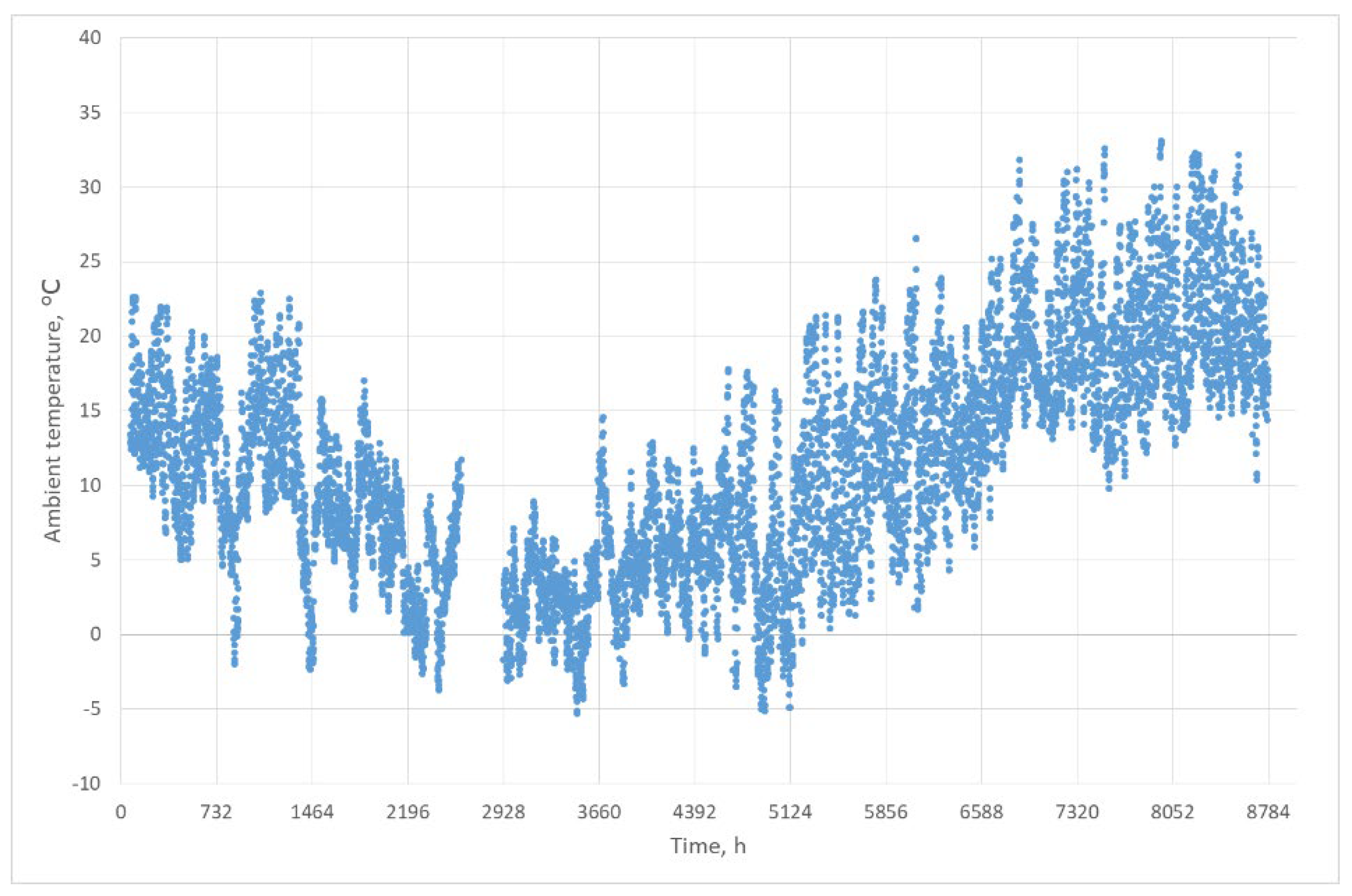
First, the observation series, ta,obs(τ), shown in Figure 2, was sorted in ascending order; then, the following was applied:
  • The time axis was normalized (index 0…Nobs − 1), according to Equation (2):
    τ ~ = τ 1 N o b s 1 0 ,   1
    for τ ~ = 1, …, Nobs; where Nobs = 8734 h (number of hours with seasonal observations).
  • Adding quality control flags (QC), extracting measurement points (tag obs = 0), and sorting in ascending order according to temperature ta,obs.
  • Fitting a polynomial of degree n in the range n = 3, 4, …, 11, according to Equation (3):
    t a , n τ ~ = k = 0 n a k τ ~ k
  • Mapping matched values to the whole timeline and filling gaps (gap = 1).
  • Inserting the complete series into the ASHP model, where the manufacturer’s characteristics P e l t a and C O P t a are interpolated exponentially.
  • Calculation of seasonal results: heat demand Q ˙ s e a s o n , electricity consumption P e l (for LWT = 35 °C and 45 °C), and the seasonal coefficient of performance SCOP. Accuracy was assessed by determining MAE, RMSE, R2, ΔQseason, ΔEel, ΔSCOP, and separately, RMSEobs and RMSEfill.
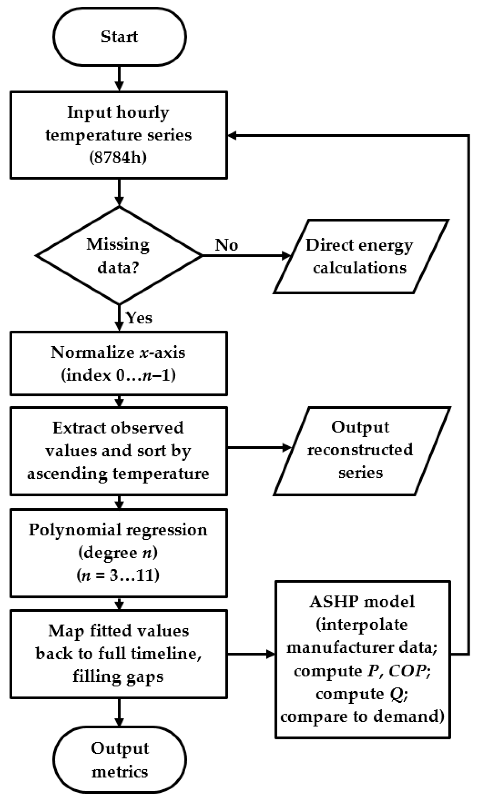
The logical data flow and the “missing data?” decision point are shown schematically in Figure 3 (normalization, ta,n fitting, mapping to the timeline, gap filling, and quality assessment). For each polynomial degree n, R2, MAE, and RMSE were calculated in three subsets Sobs (observations only), fill (fittings only), and all (entirely)—which allows the error resulting from the fit to be separated from the error of the filling itself. Additionally, MAEcold and MAEhot were reported, calculated, respectively, in the coldest S c o l d = τ S a l l : r a n k t a , r e f E and the hottest S h o t = τ S a l l : r a n k t a , r e f E (where E = 500) hours to assess sensitivity to the extremes of the temperature distribution (relevant Q ˙ h , s h , m a x and Pel,max).
Normalization τ τ ~ 0 ,   1 limits the ill-conditioning of the Vandermonde matrix when fitting polynomials and does not affect the quality of the fit [24]. The models were trained exclusively on hours with measurements (obs), after which the determined curve t a , n τ was mapped to the full time axis and limited to a physically meaningful interval [ta,min, ta,max]. Due to the risk of boundary oscillations (Runge) and overfitting at high orders, a practical range of n = 3…11 was adopted [25]; MAE/RMSE in the obs/fill/all subsets and “cold/hot” boundary indicators were used in parallel in the quality assessment. The diagram of the entire procedure is shown in Figure 3.
All models were trained exclusively on observed hours (obs) and then extrapolated to N = 8784 h; predictions were limited to the physically meaningful range [ta,min, ta,max] to avoid extreme artifacts.
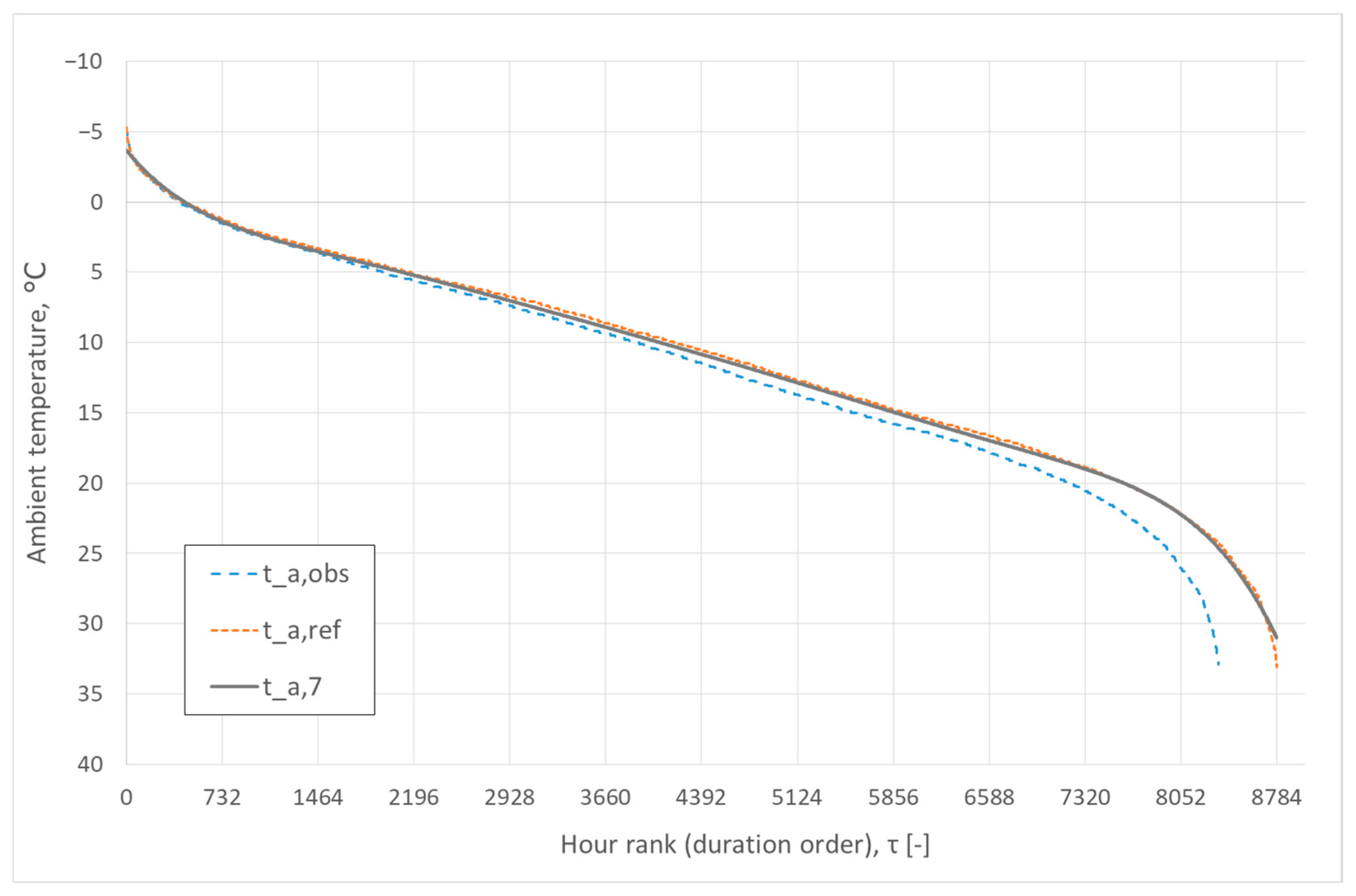
Figure 4 shows the ordered curves ta,obs, ta,ref, and ta,7. The reconstruction, e.g., n = 7, reproduces the reference curve throughout the season, with a small but significant deviation in the cold tail (bias of ∼1.6 °C between the minimums: −5.3 °C vs. −3.7 °C), which is essential from the point of view of peak power. This deviation is slight regarding MAE/RMSE, but vital for REX,max (Section 3.5).
The procedure used (axis normalization, t a , n τ fitting for n = 3…11, obs/fill, and cold/hot) ensures consistent t a , n τ profiles for further calculations. In Section 2.5, we use them to determine Q ˙ h , s h τ , Pel(τ), COP(τ), and SCOP for LWT = {35, 45} °C, and in Section 2.5, we evaluate the impact of the order n on energy metrics (ΔEel, ΔSCOP, and REX,max) and the contribution of fill error (WFEfill). COP(ta) and Pel(ta) are exponential fits to catalog maps; defrost cycles, crankcase heating, and auxiliary-resistive cut-ins are not dynamically simulated, primarily affecting the cold tail and Pel,max.

2.5. Building an ASHP Energy Model

The heat demand for a building Q ˙ h consists of the heat demand and the demand for domestic hot water preparation, according to Equation (4):
Q ˙ h τ = Q ˙ h , s h τ + Q ˙ h , h t w τ
The model assumes a linear relationship between instantaneous heat demand and outdoor temperature, ta, where x r e f , n (Equation (5)) with a design capacity of Q ˙ h , s h , m a x = 12.07 kW at ta,min = −20 °C. This value was scaled to the reference season conditions using the minimum temperature recorded during the season (−5.3 °C), which allowed for a consistent analysis of the effect of temperature reconstruction at the whole-season level. Seasonal values are calculated by discrete integration in hourly steps.
Q ˙ h , s h τ =                                       0 ,     t a , x τ   t a , b s Q ˙ h , s h , m a x · t i t a τ t i t a , m i n ,     t a , m i n < t a , x τ < t a , b s
The highest load of the season (hour no. 3488) comes from the observational part of the data (obs); therefore, all comparisons of Q ˙ h , s h , m a x refer to the same measuring point.
The following ASHP model was implemented: Silesia Term 13 kW (ST AIR 00.011 SMART MINI INVERTER 4–13). The instantaneous heating power of the ASHP is determined according to Equation (6):
Q ˙ H P t a = C O P t a · P e l t a
where the catalog maps of P e l t a and C O P t a were interpolated exponentially (Equation (7)), and Q ˙ H P t a was limited by the device’s available power.
f t a = a · e b · t a
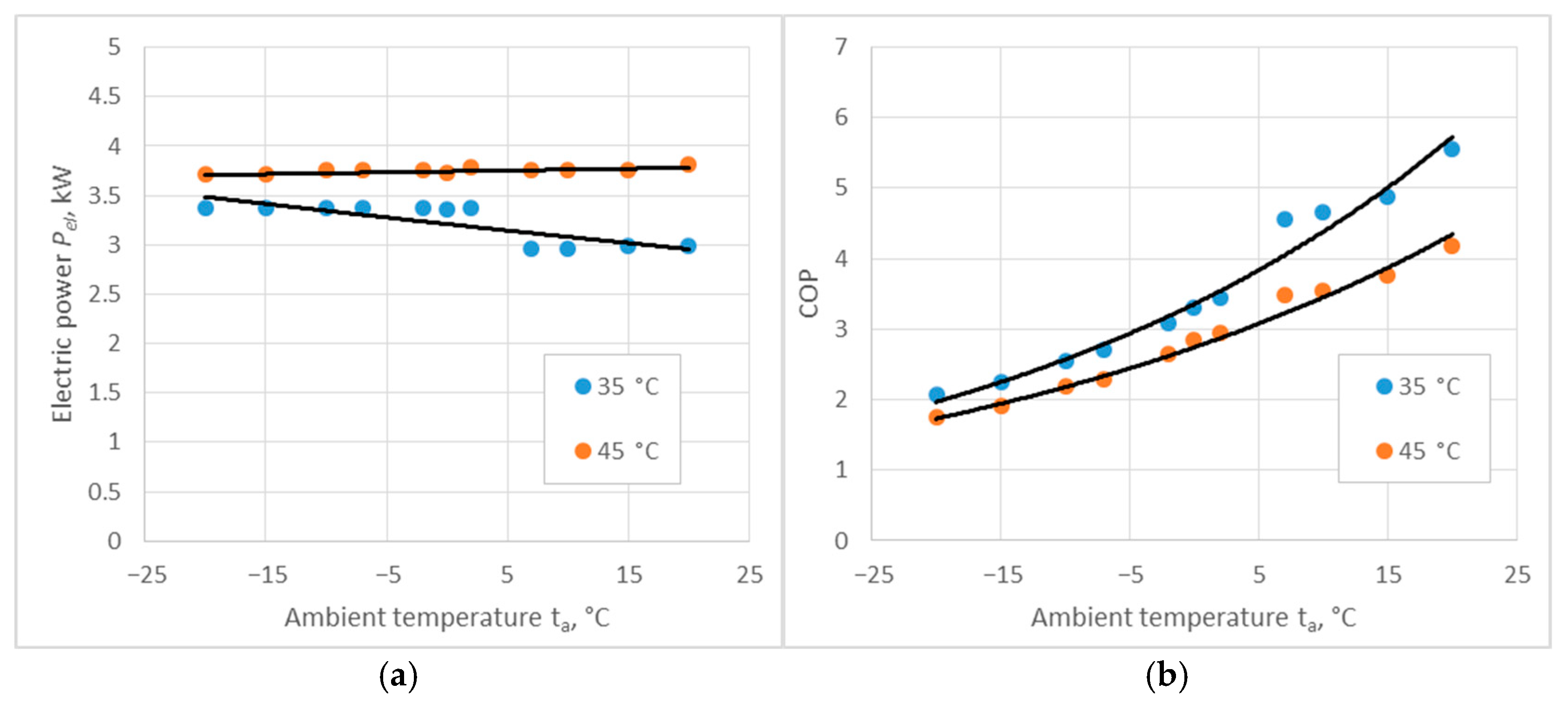
The model does not dynamically simulate defrost cycles, crankcase heating, or auxiliary-resistive heat; the maps implicitly capture these effects and are most relevant for tail behavior and REX,max. Calculations were performed for two supply water regimes, LWT = 35 °C and LWT = 45 °C, to assess the impact of supply temperature on energy consumption and SCOP. Using two LWT values (35 °C and 45 °C) made it possible to map both conditions typical for underfloor heating and domestic hot water production, significantly impacting ASHP efficiency and the frequency of auxiliary heater activation. The design parameters of the ASHP unit for selected radiator temperatures are shown in Figure 5.
The results of the approximation of the operating characteristics of both COP and electricity demand for Pel are presented in Table 1.
In this study, ambient humidity and frost/defrost cycles are not modeled as separate dynamic processes. Their aggregate influence is represented implicitly through the manufacturer performance characteristics used here—namely, COP(ta) and the electrical input/capacity versus ta—fitted in Table 1. These characteristics reflect catalog derating but do not resolve time-step defrost scheduling, crankcase-heater cycling, or humidity-driven icing intensity; therefore, transient penalties are not explicitly simulated. In practice, any residual bias from these processes is expected to concentrate in the cold tail of the outdoor-temperature distribution, primarily affecting peak electrical power and the minimum COP. Because Pel(ta) and COP(ta) are memoryless—hourly outputs depend only on the concurrent ta(τ) via manufacturer maps, with no state carried between hours—the integrated KPIs are governed primarily by the distribution of ta, including cold/hot tails, rather than short-run autocorrelation; therefore, MAEcold/MAEhot, REX,max, and WFfill are tracked to guard temporal–structure effects.
Seasonal SCOP values are calculated as the quotient of energy supplied to the building and electricity (the definition complies with the current standards for determining seasonal HP efficiency) [26,27,28].
The building parameters used to scale the thermal model are listed in Table 2: design power Q ˙ h , m a x (under ta,min conditions), internal temperature ti, heated area Af, and load model boundary parameters. These values determine the slope of the Q ˙ h , s h τ characteristic used in Equation (5) and seasonal calculations (SCOP and Eel).
The parameter Q ˙ h , h t w represents the constant demand for hot water at LWT in accordance with the adopted scenario; if the heat loss coefficient of the building is unknown, it can be omitted ( Q ˙ h , s h is modeled according to Equation (5)).
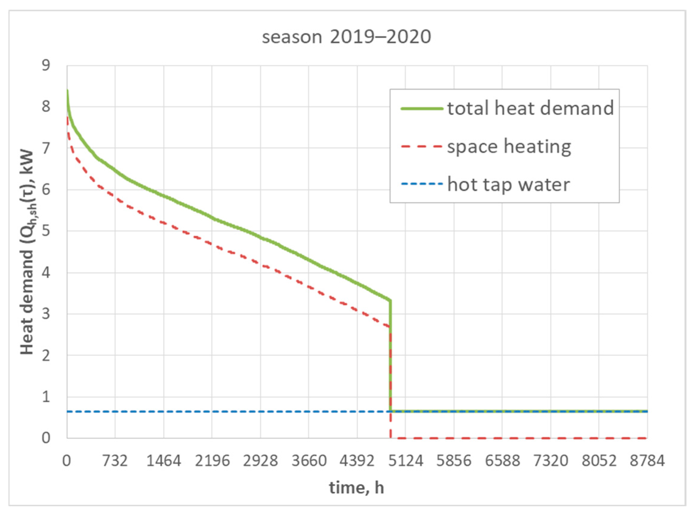
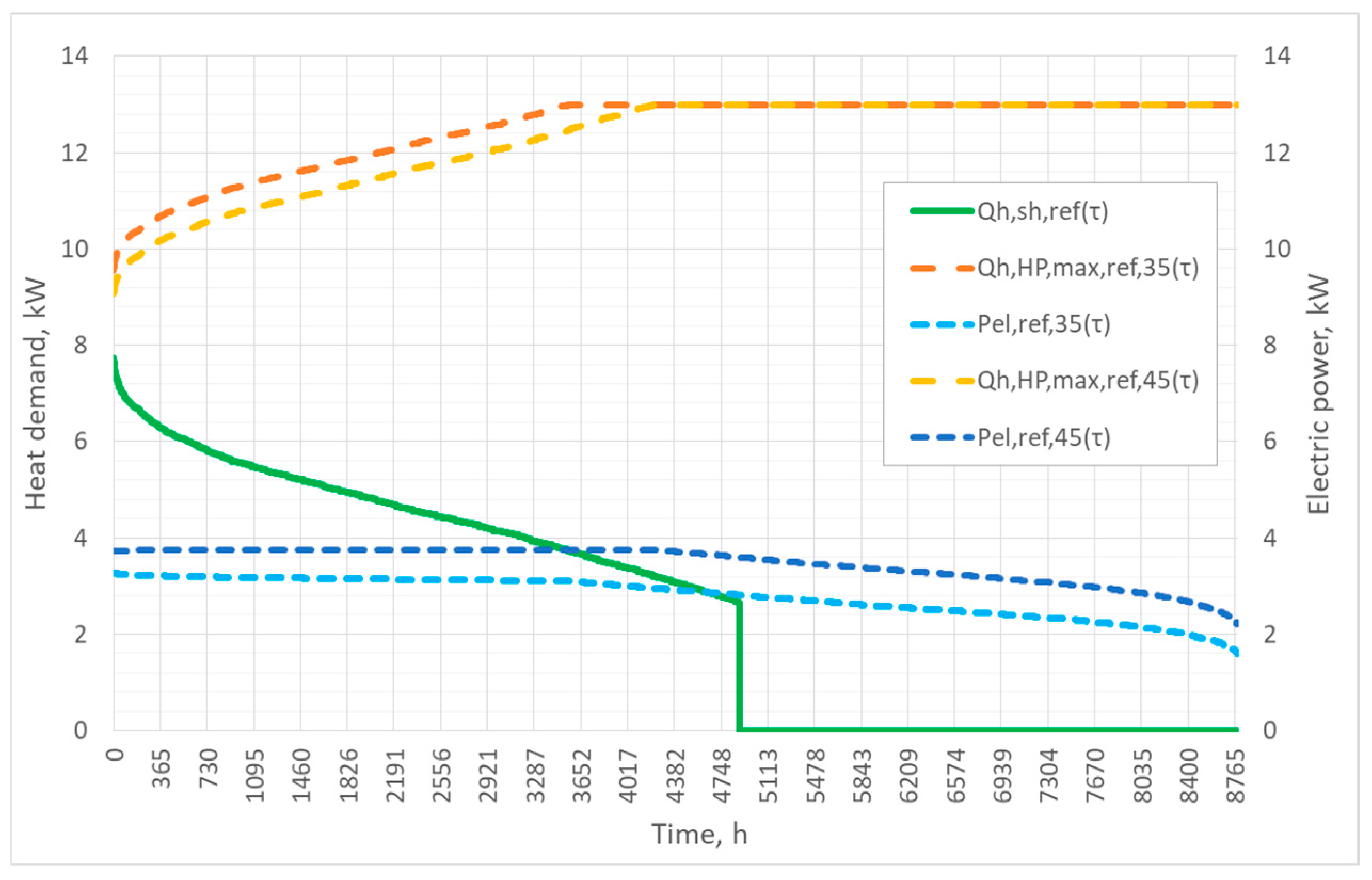
The annual load duration curve Q ˙ h , shown in Figure 6, takes into account both space heating Q ˙ h , s h and domestic hot water demand with a constant value Q ˙ h , h t w .
This curve determines the target thermal requirements of the building as a function of time. In the next step, we superimpose the ASHP characteristics onto it (Figure 7)— Q ˙ h , H P , r e f τ and P e l , r e f τ —to compare demand with heat source capabilities and calculate seasonal metrics (ΔQseason, ΔEel, and ΔSCOP) and REX,max. Here, X denotes a scalar KPI (e.g., Qseason, Eel, Pel,max, and COPmin), and Xmax, its maximum, is defined in Equation (14). Relative changes in maxima are reported as REX,max (in percent), with the general definition REX given in Equation (16).
KPI propagation from temperature to energy depends primarily on (i) the building load slope in Equation (5), and (ii) the device maps COP(ta) and Pel(ta). Steeper building slopes or maps with stronger cold-tail derating increase the sensitivity of ΔQseason, ΔEel, and REX,max to reconstruction errors; conversely, flatter slopes reduce it. A full parametric sweep is planned; here, we report the calibrated maps (Table 1) and interpret KPI changes with this dependency in mind.
Figure 7 combines information about building demand ( Q ˙ h , s h ) with source characteristics ( Q ˙ h , H P ) and supply cost (Pel) for two LWT regimes. This arrangement allows us to (i) check load coverage throughout the season (whether Q ˙ h , H P < Q ˙ h , s h for each hour); (ii) compare the impact of LWT = 35 °C vs. 45 °C on the electrical requirements Pel; and (iii) link any discrepancies to the metrics in Section 3.5 (e.g., REX,max, ΔEel, and ΔQseason). Since we do not present COP on the graph itself, its impact is indirectly taken into account by Pel(τ) and Q ˙ h , H P τ = C O P τ · P e l τ , and we report seasonal values in tables and energy metrics. We aggregate metrics hourly and seasonally, reporting ΔX (absolute value) and REX (relative value) in parallel to distinguish the temperature effect from its energy consequences. These definitions serve as the error-propagation lens from temperature reconstruction errors to energy outcomes: ΔX and REX (Equations (14)–(16)) translate ta-level deviations into ΔQseason, ΔEel, SCOP, and REX,max.

2.6. Data Reconstruction Effect Assessment Metrics

The assessment of the quality of the reconstruction includes the following:
  • Statistical accuracy: RMSE, MAE, R2—calculated separately for subsets obs, fill, and the totals all;
  • Contribution of error originating from gaps WFEfill (Equation (13));
  • Relative peak power error R E X , m a x (Equation (14));
  • Seasonal errors: ΔQseason, ΔEel, and ΔSCOP obtained by integration at hourly intervals;
  • Edge sensitivity: MAEcold and MAEhot—calculated for the 500 coldest and warmest hours.
Acceptance threshold R E Q s e a s o n 2 % was adopted as the criterion for selecting the lowest sufficient order of the polynomial. This ±2% band is an operational planning tolerance, paired with tail metrics (MAEcold/MAEhot, WFEfill, and REX,max) to guard extremes. The thresholds reflect practical KPI stability rather than formal significance tests and are read as stability bands, as shown in Section 3.2, Section 3.3 and Section 3.4; the joint behavior of Δ/RE and tail metrics conveys uncertainty. This criterion balances the compromise between energy accuracy and computational complexity, essential when planning scalable analyses for multiple meteorological locations or long multi-year series.
In the following section, we report a set of metrics for each order n: RMSE, MAE, R2 in subsets S o b s , f i l l ,   a l l , c o l d , h o t and energy indicators ΔQseason, ΔEel, ΔSCOP, REX,max. We treat Metrics MAE and RMSEs complementarily: MAE reports the average absolute deviation and is robust to outliers; RMSE penalizes large deviations and is therefore informative for tail fit and peaks [3,5]. R2 summarizes variance agreement but does not separate bias from variance; hence, we always pair it with MAE/RMSE [29]. Together with Δ/RE and REX,max (Equations (14)–(16)), these metrics translate ta-level deviations into energy outcomes.
Root mean square error (RMSE) is defined in accordance with (8):
R M S E S y n = τ S y r e f τ y n τ 2 N S
The absolute error per hour was determined as Equation (9):
M A E S y n = 1 N S τ S y r e f τ y n τ
where NS = 8784 is the number of hours in the analyzed season (1 September 2019–31 August 2020). Additionally, using the flag vector τ 0,1 (0 = measured, 1 = gap), the same pattern was applied separately to subsets “obs” and “fill”, receiving M A E Q ˙ , n , o b s and M A E Q ˙ , n , f i l l . The “all” indicator is used to assess the impact of the degree of the polynomial on the seasonal balance. At the same time, the “obs/fill” breakdown allows the source of any deviations to be located.
The Coefficient of determination R2, is defined according to Equation (10):
R S 2 y ^ i = 1 S S E S S T
where the sum of squares of residuals (SSE) is represented by Equation (11):
S S E = τ S y r e f τ y n τ 2
and the total sum of squares (SST) is represented by Equation (12):
S S T = τ S y r e f τ y ¯ r e f , S 2
where
y ^ i —modelled value (prediction) at the given time index;
y r e f —actual value of the i-th data point;
y n —value predicted by the model;
y ¯ r e f , S —average actual value, y ¯ r e f , S = 1 N S τ S y r e f τ ;
N S —number of observations.
In each version of R2, we take y r e f as reference values (e.g., ta,reft or Q ˙ h , s h , r e f ), and y n as the corresponding values from reconstruction n; we report R2 separately for Sobs, Sfill, and Sall.
The W F E f i l l indicator shows what part of the total MAE error comes exclusively from filled hours (percentage share of error in gaps in total MAE)—an original metric, reported alongside MAE/RMSE so as not to overestimate the accuracy obtained on well-observed parts. In this paper, we report W F E f i l l for the Q ˙ load error (Equation (13)), i.e., a measure of the share of error from filled hours in the total MAE; the temperature variant is not used here.
W F E f i l l = N f i l l N a l l · M A E Q ˙ , n , f i l l M A E Q ˙ , n , a l l · 100 %
where Nfill is the number of hours with a gap (after filling); and Nall = N is the number of hours in the season.
This indicator made it possible to determine the extent to which errors in temperature reconstruction result directly from missing data segments and the extent to which they result from the overall polynomial fit to the complete series. A WFEfill value close to the proportion of hours with gaps (here, approx. 5%) means that the error “generated” by the fill is comparable in scale to the proportion of gaps themselves; significantly higher values indicate a dominant error cost in the Sfill area.
The relative peak error (REX,max) is defined as Equation (14):
R E X , m a x , n = X m a x , n X m a x , r e f X m a x , r e f · 100 %
where Xmax,ref is the maximum in the reference series; and Xmax,n—maximum in the reconstructed series (evaluated at the same time step).
In the following section, we use abbreviated notation R E X , m a x , where X Q ˙ h , s h , m a x ,   N e l , m a x ,   C O P m i n . A positive sign indicates an overestimation relative to the reference (see Equation (14)). This convention expresses the deviation in the modeled variable X concerning the reference series; alternatives normalized by Xmax,n were rejected to avoid ambiguity.
For LWT = {35, 45} °C we report (i) E e l = P e l , n P e l , r e f , REX, (ii) ΔPel,max and REX,max, (iii) ΔSCOP and RESCOP—separately for each LWT, because the COP map and power limitations depend on the supply level. We refer SCOP and its interpretation to the standard definition (test framework and seasonal aggregation method) [19].
Seasonal differences (absolute values Δ) are defined in accordance with Equation (15):
X n = X n X r e f
where X means one of the full-season quantities: electricity Eel, usable energy/heat Qseason, or derivative indicators (i.e., SCOP).
ΔXn is reported in parallel with REX,n, which provides an absolute and relative scale of seasonal differences and facilitates the assessment of the significance of differences from an operational perspective.
The relative seasonal error (REX) is represented by Equation (16):
R E X , n = X n X r e f X r e f · 100 %
For REX,n, we use the same convention (Equation (14)): positive values indicate overestimation relative to the reference, negative values indicate underestimation. In practice, we use Equation (16) for X = Qseason, where Qseason is the sum of hourly power i = 1 N Q ˙ h , s h τ in the season (see Equation (5)).
The MAE in the tails of the distribution (cold/hot) is defined sequentially according to Equations (17) and (18):
M A E n , c o l d = 1 N c o l d τ S c o l d y τ y ^ n τ
M A E n , h o t = 1 N h o t τ S h o t y τ y ^ n τ
where Scold and Shot are sets of hours comprising the 500 coldest and 500 warmest hours of the season, respectively. E = 500 ≈ 6% of the season, corresponding to approximately three weeks in the cold/warm tail.
Their complementarity justifies the selection of metrics: MAE and RMSE measure absolute error in different standards, R2 assesses the conformity of the curve shape and energy indicators (ΔQseason, ΔEel, and ΔSCOP), and REX,max allows temperature accuracy to be translated into practical effects for the ASHP model. We treat evaluation thresholds (e.g., ±2% for ΔQseason) as the selection criterion of the “lowest sufficient” order of the n-th degree of the polynomial. We control sensitivity to the extremes of the distribution by MAEcold and MAEhot calculated for the 500 coldest and 500 warmest hours, respectively (Scold and Shot).
The metrics and scenarios defined above (LWT = {35, 45} °C) are used in the Section 3, comparing orders n = 3…11 statistically (obs/fill/all, “cold/hot”), and energetically (ΔQseason, ΔEel, ΔSCOP, and REX,max), which allow for identification of the lowest polynomial order that meets the criterion R E Q s e a s o n 2 % .

3. Results

This chapter presents the impact of the degree of the polynomial n used to reconstruct the hourly outdoor temperature profile on the energy indicators of the air-source heat pump (ASHP) model in two operating regimes LWT. The analysis is performed in the subsets Sobs, Sfill, and Sall, and the boundary zones Scold and Shot, according to the definitions and workflow described in Section 2. The device characteristics COP(ta) and Pel(ta) were approximated by exponential functions calibrated on catalog data. The following sections present, in order: (I) the quality of temperature reconstruction (MAE, RMSE, and R2) as a function of n; (II) the consequences for the thermal loads and peak power of the building/device; and (III) the seasonal effects (Eel, SCOP, and Pel,max) in both LWT regimes. The selection of the “lowest sufficient” order was based on the acceptance threshold for R E Q s e a s o n from Section 2. Graphical summaries accompany the tables: Figure 8, Figure 9, Figure 10, Figure 11, Figure 12 and Figure 13 cover RMSE/MAE/R2 and Δ summaries; Figure 14 and Figure 15 present seasonal Δ/RE (Qseason, Eel, and SCOP) for both LWT regimes; Figure 16 and Figure 17 show peak-power REX,max, and WFEfill.

3.1. Accuracy of Temperature Profile Reconstruction ta
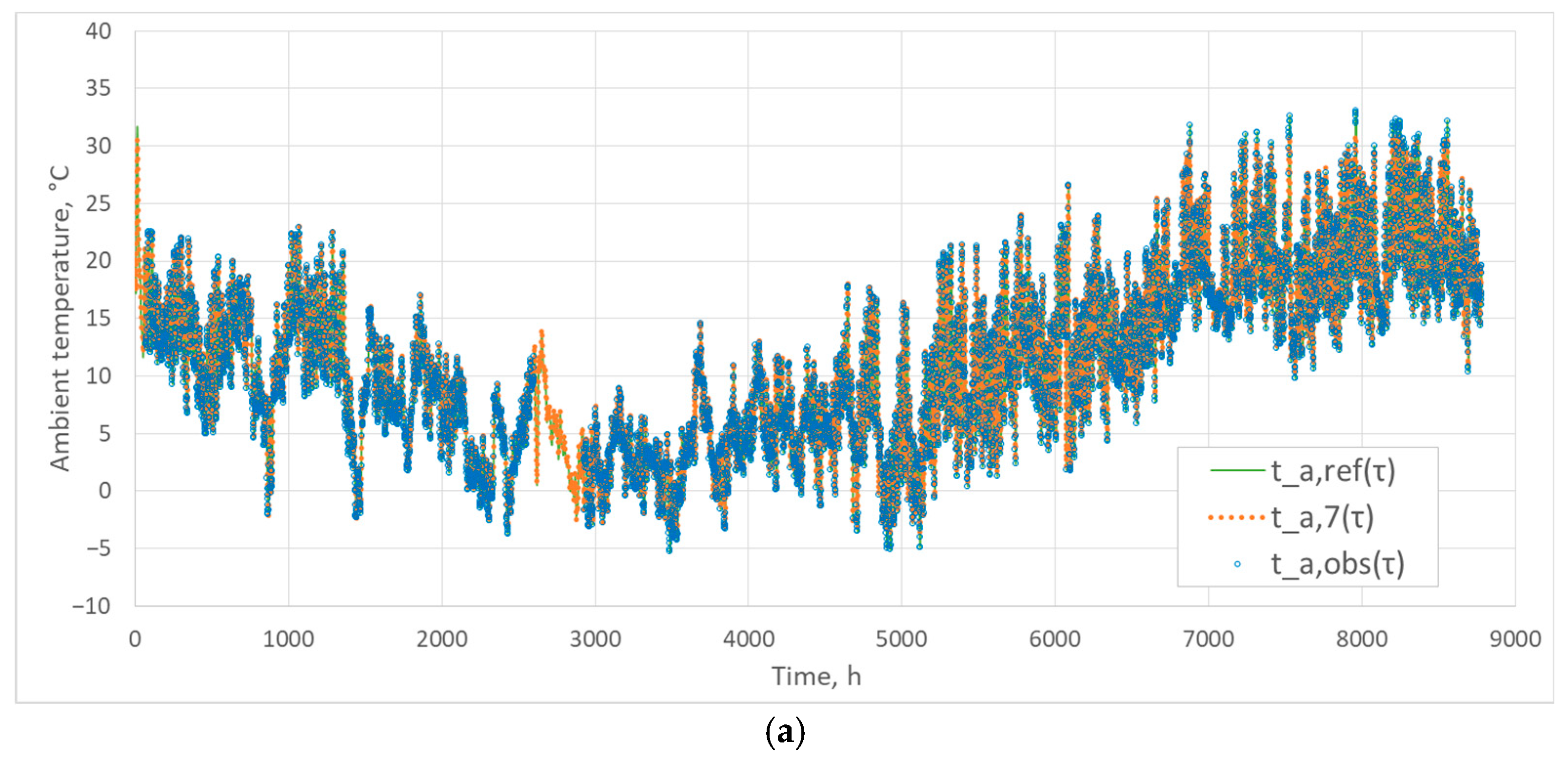
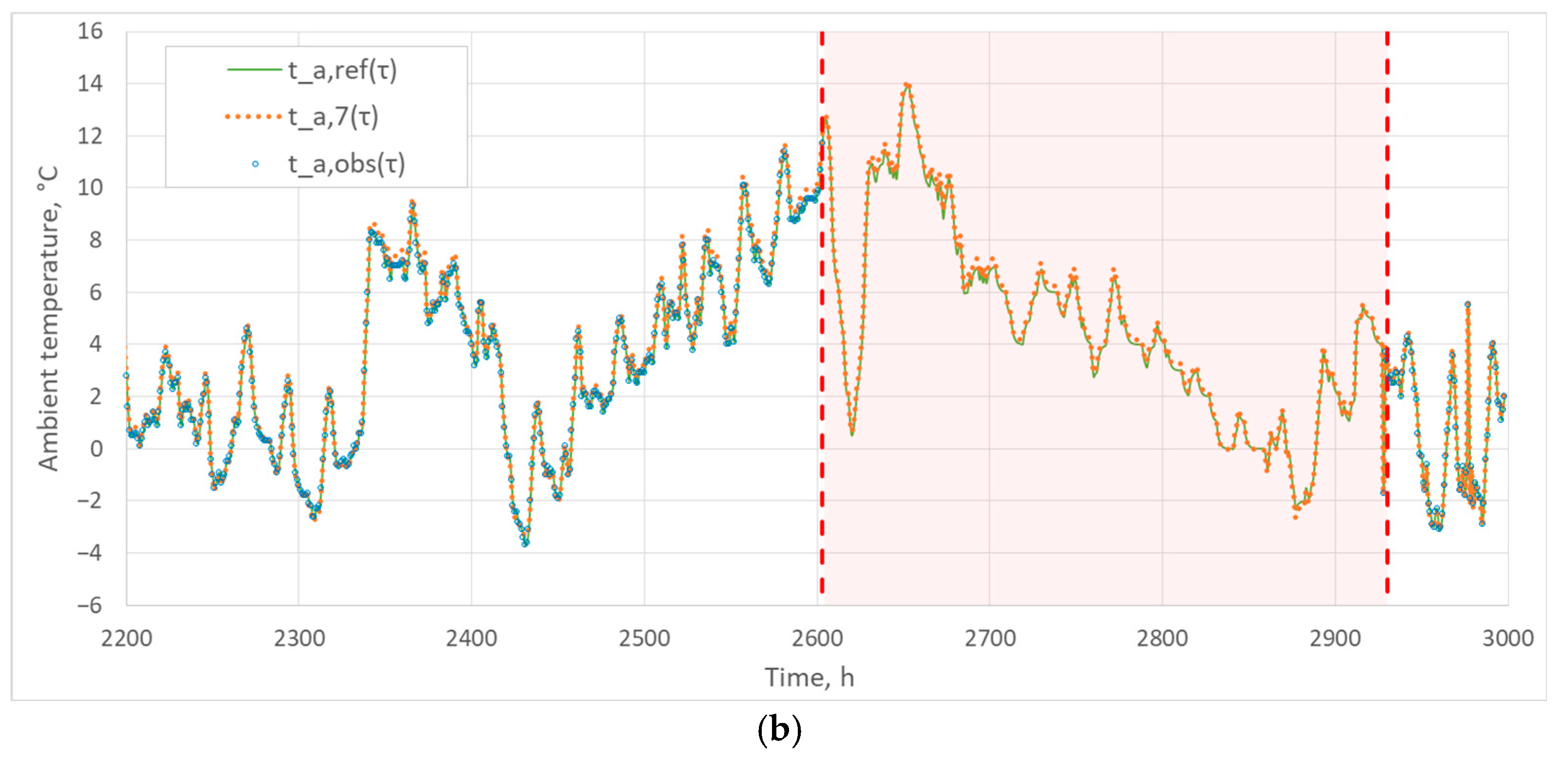
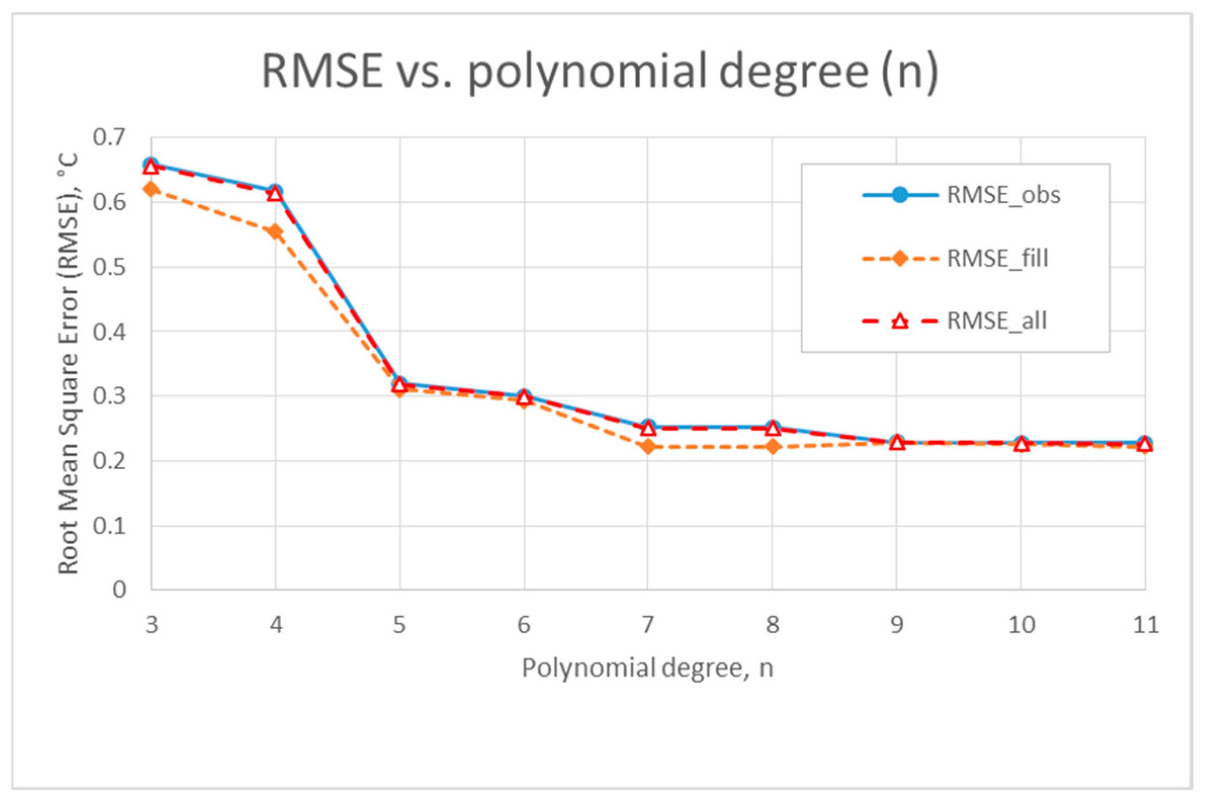
This section summarizes the accuracy of the hourly outdoor temperature profile reconstruction ta as a function of the polynomial degree n = 3…11. The presentation includes metrics. The presentation contains metrics RMSE and MAE calculated in parallel in subsets Sobs, Sfill, and Sall, and an analysis of the distribution “tails” Scold and Shot. The additional graph shows the R2. A summary of extreme deviations is provided at the end of the section Δ = [Δavg, Δmin, Δmax]. To illustrate chronology after mapping, Figure 8a shows the full-year time-domain overlay of ta,ref(τ), ta,7(τ), and ta,obs(τ); Figure 8b zooms into a representative real gap (324 h), shading the missing interval and showing overlaps at both ends.
Figure 9 shows the RMSE curve as a function of n; errors for measurement points were reported separately (RMSEobs), for refilled points (RMSEfill), and for the entire series (RMSEall). RMSE plateaus by n ≈ 7 in all subsets; the most significant gains occur from n = 4→5, then diminish.
Figure 8. Time-domain views of the reconstruction: (a) Full-year overlay: thin line = ta,ref(τ), dashed line = ta,7(τ), markers = ta,obs(τ). (b) Zoom across a representative real gap (shaded) with overlaps at both ends; alignment at gap boundaries illustrates mapping back to time.
Energies 18 05547 g008aEnergies 18 05547 g008b
Figure 9. Dependence of RMSE on the degree of the polynomial n.
Energies 18 05547 g009
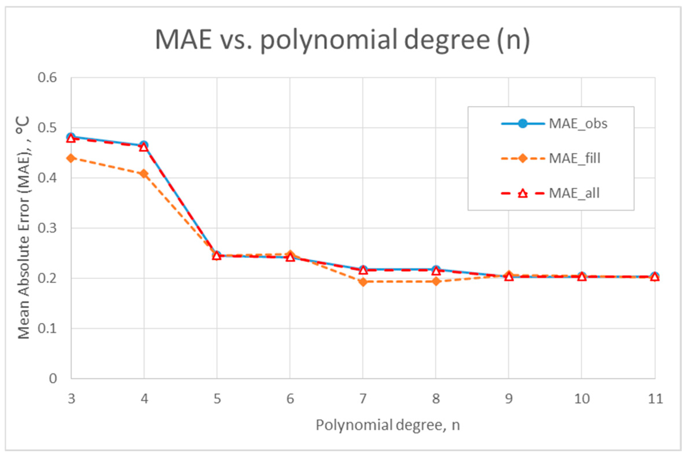
Figure 10 compares MAE as a function of n for the same subsets, using the same notation convention. MAE follows the same trend as RMSE; Sfill converges slightly later than Sobs.
Figure 10. MAE is in the function n for Sobs, Sfill, and Sall.
Energies 18 05547 g010
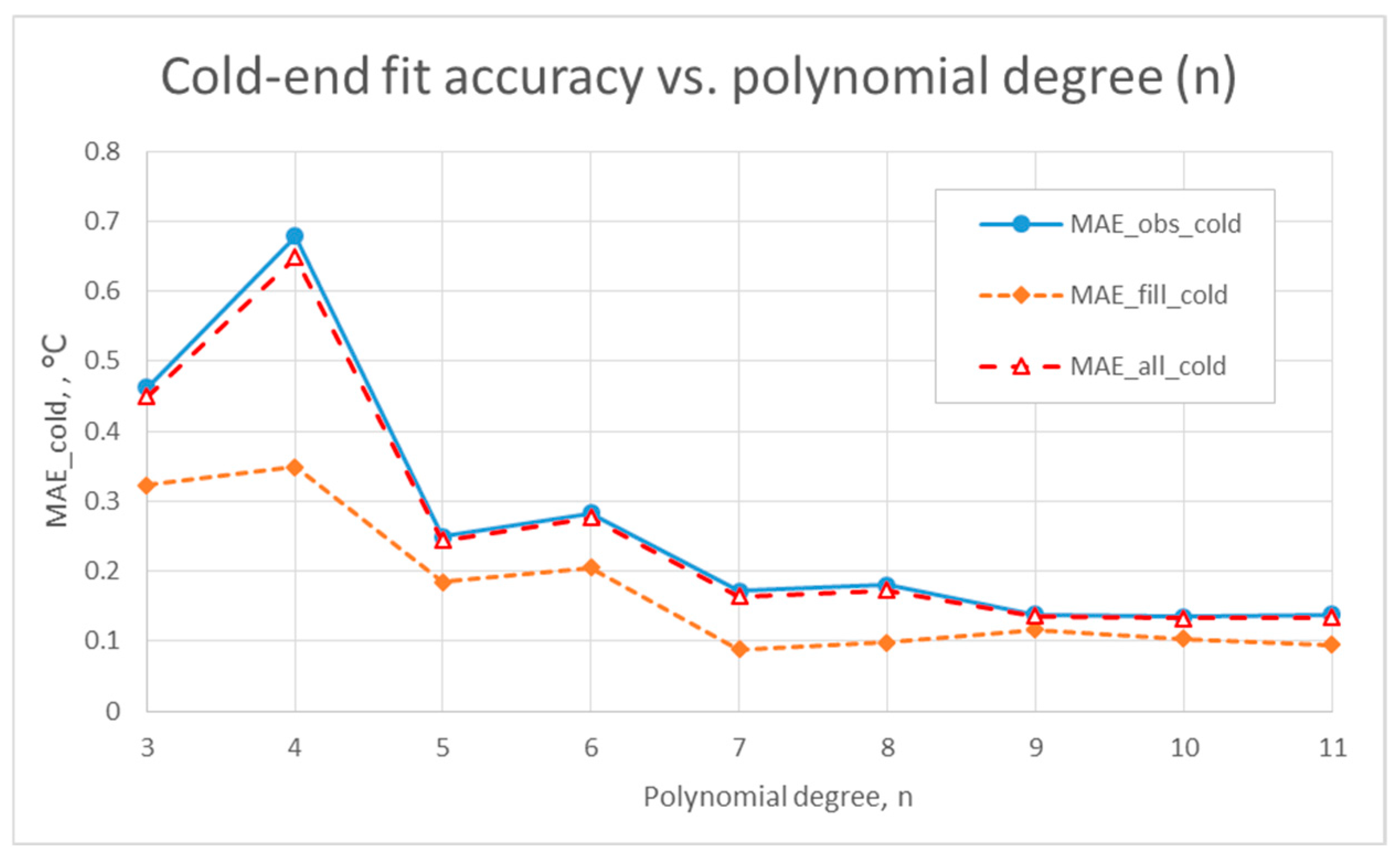
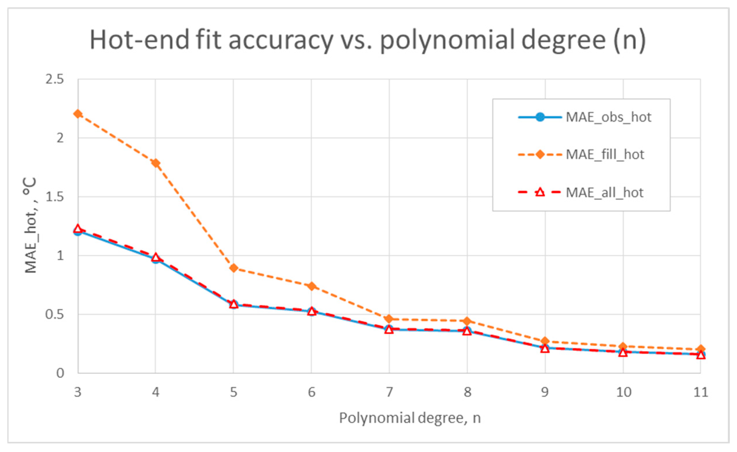
Figure 11 and Figure 12 show the MAE values for the season’s 500 coldest and 500 warmest hours, respectively. Cold-tail MAE stabilizes for n ≥ 7; improvements beyond n = 7 do not materially affect energy KPIs. Hot-tail MAE is low across n and stabilizes early; changes above n = 7 are negligible.
Figure 11. MAE for “cold tail” (first 500 h of the season): Sobs,cold, Sfill,cold, Sall,cold in the function n.
Energies 18 05547 g011
Figure 12. MAE for “warm tail” (last 500 h of the season): Sobs,hot, Sfill,hot, Sall,hot in the function n.
Energies 18 05547 g012
Figure 13 presents R2 calculated separately for Sobs, Sfill, and Sall as a function of n. R2 remains > 0.99 for all degrees; hence, Δ/RE metrics drive the degree selection rather than R2.
Figure 13. R2 in the function n.
Energies 18 05547 g013
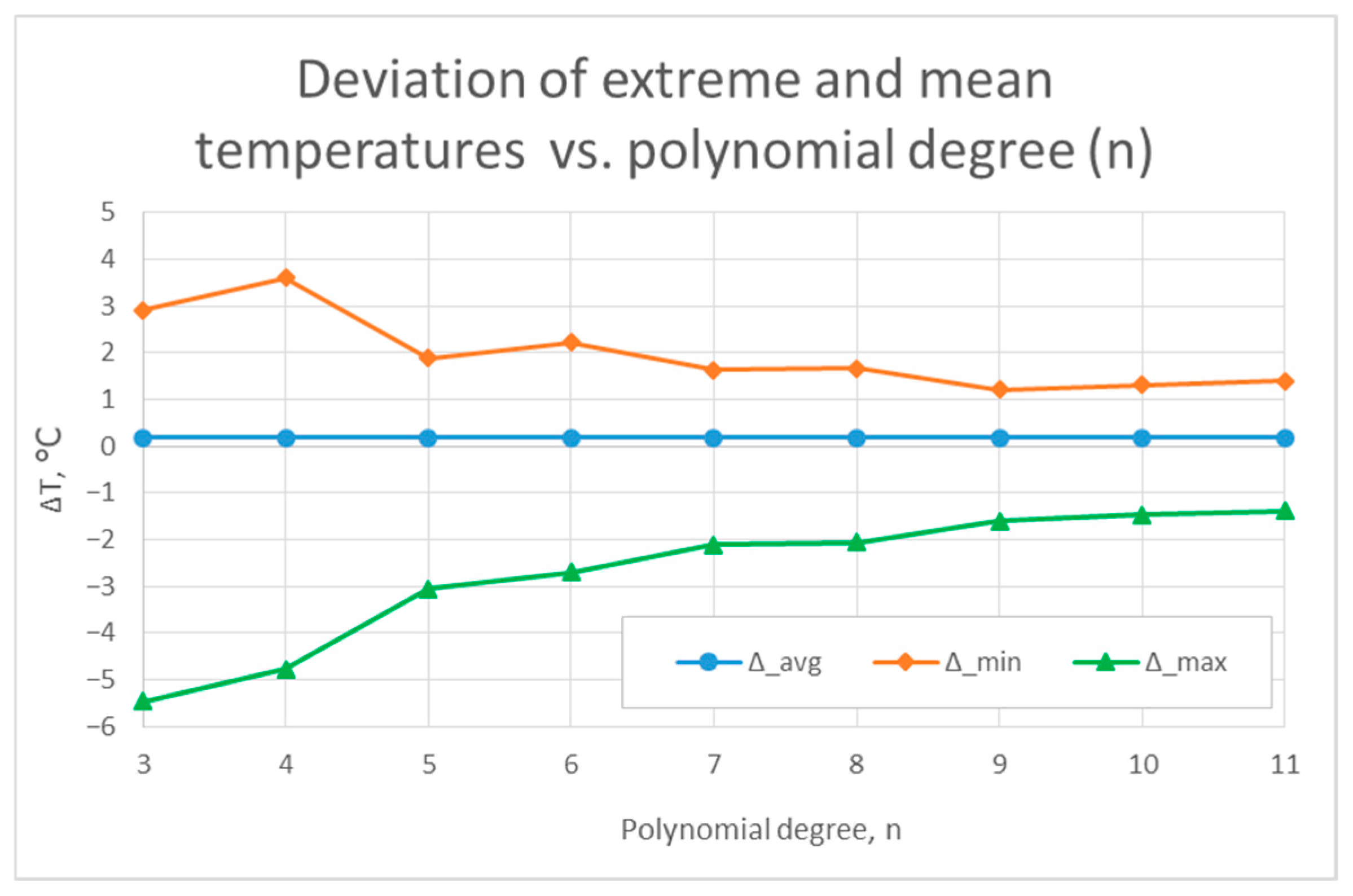
A summary description of the values Δ = [Δavg, Δmin, Δmax] is provided in Figure 14. In this study, τ = t a , n τ t a , r e f τ ; Δavg was assumed; Δavg denotes the average for the entire season (N = 8784 h), while Δmin and Δmax denote the extreme values of the difference within the season, respectively. Seasonal mean bias is slight; extremes narrow with n and stabilize by n ≈ 7.
Figure 14. Absolute differences (Δ) ta between reconstruction and reference in the n-th degree function for the entire seasonal series (Sall, N = 8784 h). Different positive values indicate a warmer reconstruction than the reference. (The graph supplements the “cold/hot” summaries, average shift, and range of extremes for the entire season.).
Energies 18 05547 g014

3.2. The Impact of n on the Thermal Load of a Building
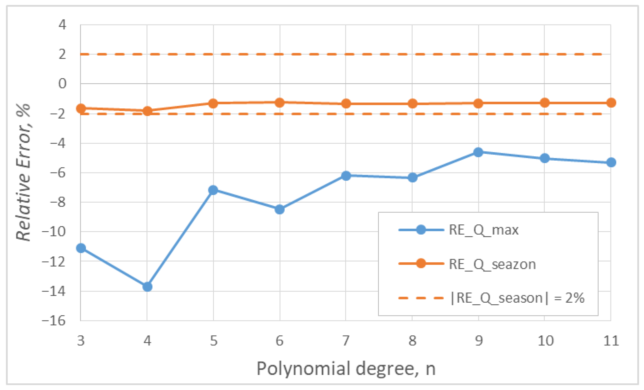
This section presents the effects of the degree of the polynomial n on the thermal load of a building. The peak heat demand value Q ˙ h , s h , m a x was compared with the seasonal effective energy ΔQseason determined from profiles t a , n τ for n = 3…11. For comparability, the maximums arise at the same time of the season Sobs (3488 h), which allows for a direct comparison of peak values, and the results are presented in pairs Δ/RE (Table 3).
Figure 15 shows the relative errors R E Q ˙ h , s h , m a x and R E Q s e a s o n in the function of degree n, with lines ±2% indicating the acceptance band for R E Q s e a s o n . Seasonal Δ and RE for Qseason lie within planning-level tolerances for all n; changes beyond n = 7 are immaterial.
Figure 15. RE in the function n: R E Q ˙ h , s h , m a x and R E Q s e a s o n on a shared Y-axis. The dashed lines ±2% indicate the acceptance band R E Q s e a s o n ; where RE_Q_max ≡ R E Q ˙ h , s h , m a x .
Energies 18 05547 g015
All R E Q s e a s o n values fall within the range of ±2%; the smallest absolute value was recorded for n = 6 (−1.24%).

3.3. Impact of n on ASHP Energy Indicators
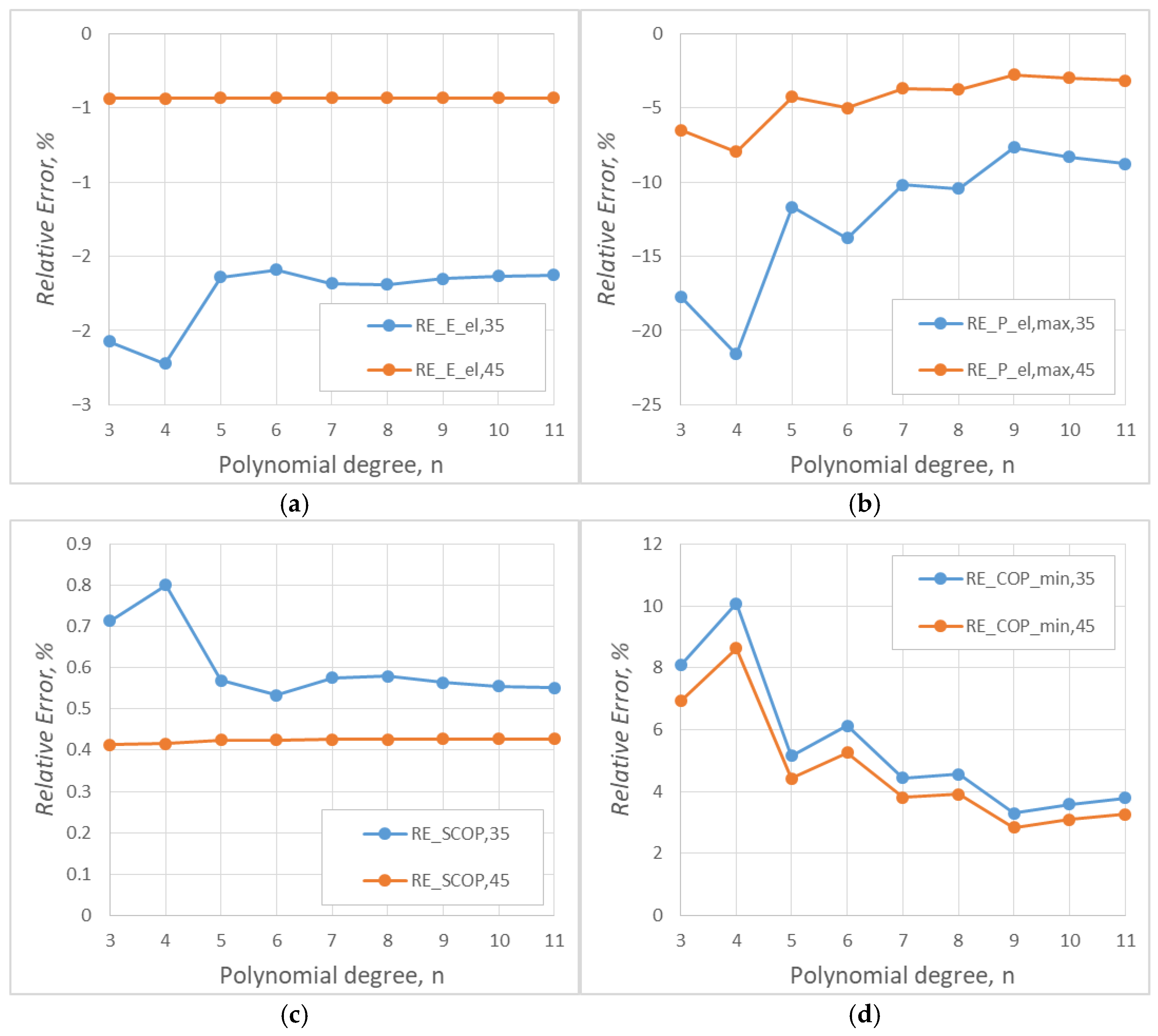
Variations in Eel, SCOP, Pel,max, and COPmin, are presented in Table 4 and Figure 16. Seasonal Δ and RE for Eel and SCOP stabilize from n ≈ 5; for Pel,max and COPmin from n ≈ 7; changes above 7 for all trends are insignificant.
Figure 16. RE vs. polynomial degree n for two LWT regimes (35 °C, 45 °C): (a) R E E e l , (b) R E P e l , m a x , (c) RESCOP, (d) R E C O P m i n .
Energies 18 05547 g016
The differences visible in the charts above and their implications are discussed in Section 4.

3.4. Sensitivity of the Method to Cold/Hot “Tails”
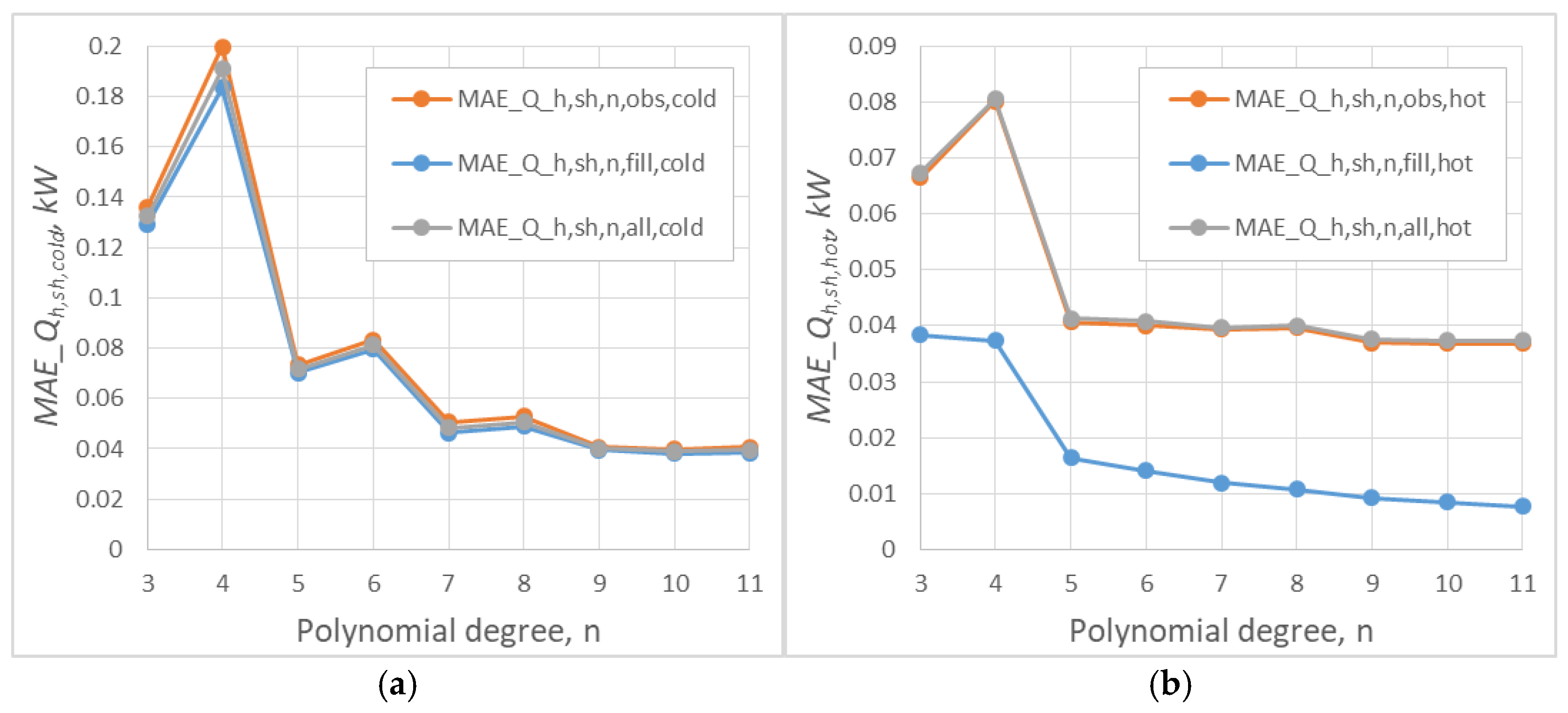
Since the technique is most sensitive at the extremes of the temperature distribution, the sensitivity of the method was assessed in the boundary zones of the temperature distribution: Scold and Shot. The MAE was calculated separately in Sobs, Sfill, and Sall.
For Scold, the values of M A E Q ˙ h , s h in low n, the most significant value decreases significantly at n ≥ 7. Shot is also stabilizing starting from n ≥ 7. Detailed MAE waveforms in the “tails” are shown in Figure 17. The local maximum separation of the curve Sfill in relation to Sobs and Sall for n = 4 is shown in Figure 17b.
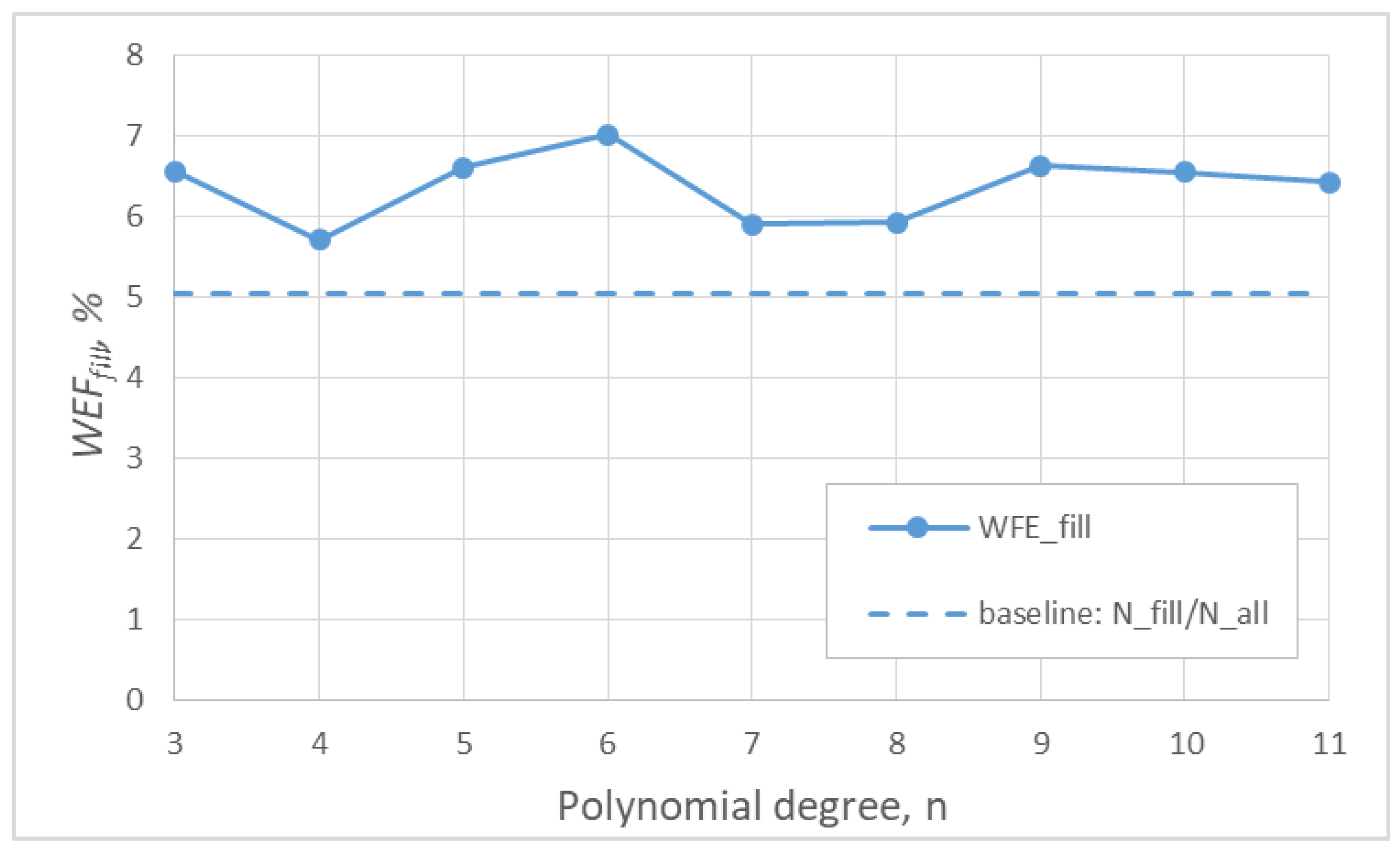
The WFEfill indicator synthesizes the global share of error from hours supplemented in MAEall for Q ˙ h , s h . The WFEfill values close to the proportion of gaps (Nfill/Nall) mean that the error from gaps does not dominate the total error. Significantly higher values indicate that errors in the Sfill subset increase the total error (MAEall). In this sample, the smallest WFEfill (i.e., closest to the Nfill/Nall line) was obtained for n = 4, 7, and 8 (Figure 18), which is consistent with the fact that the Shot tail covers only 5.1% of the season and does not determine the share of error on an annual basis.
Figure 17. MAE for Q ˙ h , s h in the edge zones of the distribution—(a) Scold, (b) Shot—as a function of the degree of the polynomial n. Three curves are shown: Sobs, Sfill, and Sall.
Energies 18 05547 g017
Figure 18. WFEfill indicator as a function of degree n for Q ˙ h , s h . Baseline N f i l l / N a l l · 100 % as a reference point (proportion of completed hours).
Energies 18 05547 g018

3.5. Choosing the Lowest Sufficient Degree n

The selection of the lowest sufficient degree was based on four criteria:
  • I—error acceptance threshold R E Q s e a s o n 2 % . Those that meet this criterion are identified.
  • II—threshold for stabilizing energy indicators. For each X R E E e l , R E P e l , m a x , E R S C O P , R E C O P m i n and both regimes, LWT = 35 °C, 45 °C, the incremental change is compared R E X n = R E X n R E X n 1 R E E e l 0.15   p p , R E P e l , m a x 2.0   p p , E R S C O P 0.10   p p , R E C O P m i n 1.0   p p for both LWT and is marked as follows (pp—percentage points):
    • (✓)—if the criteria are met simultaneously;
    • (△)—if only one of the thresholds is exceeded by 50%;
    • (—)—all other cases.
  • III—stabilization of M A E Q ˙ for tails in Sall and is marked as follows:
    • (✓)—if M A E a l l n M A E a l l n 1 0.05   k W AND relatively ≤ 5%;
    • (△)—if M A E a l l n M A E a l l n 1 0.10   k W OR relatively ≤ 10%;
    • (—)—all other cases.
  • IV—contribution of missing data WFEfill. For b = (Nfill/Nall)⋅100% it is marked as follows:
    • (✓)—if W F E f i l l n b 1.0   p p ;
    • (△)—if W F E f i l l n b 2.0   p p ;
    • (—)—all other cases.
The thresholds discussed are operational and were adopted a priori based on two premises: (I) stabilization of the curves in Figure 15 and Figure 16, and (II) energy metric levels. The thresholds do not result from statistical significance tests, but reflect the practical level of the model’s insensitivity to further increases in n. The fulfillment of the four decision premises from Figure 14, Figure 15, Figure 16 and Figure 17 is summarized in Table 5.
Within this study’s scope, all considered n meet R E Q s e a s o n 2 % yet n = 7 is the first degree at which conditions I–IV are met simultaneously (Table 5). For n = 7, all reported KPIs fall within the tolerances, and increments to n > 7 produce no material changes, indicating diminishing returns and a higher overfitting risk, as low degrees underfit the cold-tail slope. In contrast, higher degrees mainly reshape tails with little effect on seasonal integrals.

4. Discussion

The consequences of selecting the reconstruction degree n for ASHP energy indicators in two LWT regimes are discussed below, considering the analysis of temperature distribution and the impact of data reconstruction. The discussion is based on criteria I–IV (Figure 14, Figure 15, Figure 16 and Figure 17; Table 5) and the metrics definitions from Section 2.6.

4.1. Quality of Temperature Reconstruction and Energy Effect

The obtained profiles t a , n τ ensure high compliance with the reference series, with the quality increment decreasing significantly for n ≥ 7. The translation into building load is confirmed by R E Q s e a s o n 2 % for all analyzed degrees and slight changes in R E E e l and E R S C O P . This means that further increasing the n above the average values does not bring any material energy benefits in the case under consideration.
Increasing the degree of the polynomial improves the representation of daily and weekly variability in the profile t a τ , which directly translates into stabilization of MAE/RMSE in the Sobs, Sfill, and Sall sets. The most significant increase in quality occurs when moving from n = 4 to n = 5, while for n ≥ 7, the benefits diminish.
Very high consistency (R2 > 0.99) was maintained throughout the studied range. From the building energy efficiency point of view, the smoothness of the entire t a τ distribution is crucial, rather than the local adjustment of individual episodes. Hence, all the reconstructions considered meet the acceptance band R E Q s e a s o n 2 % ; R E E e l and E R S C O P remain low. Further increases in n do not translate into measurable energy gains in the analyzed case.
This study does not benchmark alternative gap-filling families (linear/spline, ARIMA, ML). In this case, the contribution is orthogonal: the degree of the polynomial n was isolated as a single design variable in an ordered domain, and its selection was made repeatable through KPI propagation. Comparative baselines are left for follow-on replication using the same decision rule.

4.2. LWT Regimes and KPI Sensitivity

Differentiation of LWT modifies the sensitivity of indicators to reconstruction t a : for LWT = 45 °C, values of R E E e l are similar to −0.43%, while for LWT = 35 °C, deviations in R E E e l and R E P e l , m a x are clearly larger. At the same time E R S C O P and R E C O P m i n remain within narrow ranges for both regimes, which confirms the stability of overall efficiency with respect to the choice of n. Interpretatively, this means that at lower supply temperatures, changes in the load profile resulting from reconstruction t a are more easily “visible” in seasonal energy and peak power, while at 45 °C, remain secondary in nature. At the same time, E R S C O P and R E C O P m i n remain within narrow ranges for both regimes, confirming the stability of the device’s overall efficiency concerning the choice of n. Energy sensitivity varies significantly between regimes. For 35 °C, ranges were recorded: R E E e l 2.22 % ,     1.63 % , R E P e l , m a x 21.59 % , 7.65 % , in narrow ranges of R E S C O P and R E C O P m i n . For 45 °C, the range is R E P e l , m a x 7.59 % , 2.75 % . These quantitative differences confirm that the selection of n has a stronger “transfer” effect on the energy and peak power in the system LWT = 35 °C than in the system LWT = 45 °C.
The rooms are heated exclusively by underfloor heating, so most of the ASHP’s operating hours fall within the regime LWT = 35 °C, while LWT = 45 °C mainly concerns episodic DHW preparation cycles. In this sense, greater sensitivity of indicators at 35 °C has greater operational significance than the differences observed at 45 °C.

4.3. Edge Sensitivity and the Contribution of Complementary Hours Error

Analysis of the “tails” of the temperature distribution confirms that M A E Q ˙ h , s h stabilizes for n ≥ 7 for Scold and Shot. Visible local deviation of the Sfill in Shot for selected degrees n, it does not escalate the whole-season error, which is reflected in the indicator WFEfill (values closest to Nfill/Nall baseline are for n = 4, 7, 8). With a “warm tail” of ~6% of the season, the contribution of the error from the hours filled in remains secondary to M A E a l l . Therefore, raising the degree of the polynomial above 7 does not significantly reduce the edge sensitivity. This pattern supports the ordered-curve reconstruction: for n ≥ 7 the edge-sensitivity metrics stabilize despite the lack of explicit time-series dependence.
As humidity- and defrost-related transients are not explicitly simulated, cold-tail indicators (e.g., peak electrical power and minimum COP) should be interpreted with this modeling scope in mind. In the present case, these effects may modestly accentuate cold-tail deviations without altering the qualitative patterns discussed above. A simple sensitivity (cold-tail COP penalty and auxiliary cut-in) leaves the n ≈ 7 degree selection unchanged in directionality, while increasing R E P e l , m a x as expected.

4.4. Justification for Selecting the Minimum Sufficient Degree n

The lowest degree of the polynomial n was accepted when the thresholds were met in both LWT regimes. The first degree at which criteria I–IV were simultaneously met is n = 7. Further increasing the degree does not bring about any significant improvement.
Against time-series baselines (e.g., ARIMA/splines/ML), the ordered-curve fit is preferable here because gaps are short and ASHP relations are memoryless; under dense/extended gaps, time-series or reanalysis debiasing would become preferable. The degree-selection criterion applies to the polynomial reconstruction implemented in the previously published ASHP planning tool [1,2]. The observed saturation at n ≈ 7 reflects that short, scattered gaps and memoryless Pel(ta)/COP(ta) relations make KPI integrals depend mainly on the temperature distribution; beyond this point, extra degrees primarily reshape tails with negligible KPI impact. Replication across additional climates (including warm/cold subperiods) and ASHP types is planned; using a single climate year here keeps the analysis compact and makes the criterion auditable before replication.
Mechanistically, the saturation at n ≈ 7 follows how degree n reshapes the ordered temperature curve. For n ≤ 5, the cold tail is overly smoothed, which reduces the frequency of very low ta and leads to underestimation of Q ˙ h , s h , m a x and Pel,max; for n ≥ 10, local Runge-type oscillations may appear, artificially shifting hours near control thresholds. The stabilization of MAEcold/MAEhot and the plateaus of R E E e l , E R S C O P , and R E P e l , m a x observed from n ≥ 7 (see Figure 15, Figure 16 and Figure 17) indicate that this is the lowest degree at which tail bias and oscillation risk are simultaneously controlled within the ±2% planning band.
The “lowest sufficient degree via KPI propagation” principle is generic and can inform other analytics pipelines (e.g., battery SOC estimation), provided the domain-specific KPIs and tails are defined.

4.5. Limitations and External Baselines (Method Positioning)

Time-series-aware baselines (splines on time, ARIMA/state-space, ML, and reanalysis debiasing) are valuable when chronology carries predictive information or missingness is dense. Here, gaps are short and scattered (5.1%), and Pel(ta)/COP(ta) are memoryless maps; therefore, KPI integrals are governed mainly by the ordered distribution of ta. Under this regime, the degree-selection criterion is based on ΔQseason, ΔEel, SCOP, R E P e l , m a x , MAEcold/MAEhot, and WFEfill, which identify n = 7 as the lowest sufficient degree. Broader comparisons are planned in the upcoming multi-climate replication that reuses the same criterion.

5. Conclusions

Based on the analysis of the results, the minimum sufficient degree of reconstruction of temperature data n was identified, and the sensitivity of ASHP energy indicators to n in two LWT regimes was determined. The most important practical conclusions and implications for the selection of n in similar applications are summarized below:
  • Degree n = 7 is the lowest sufficient according to the criteria I–IV;
  • Since in a building with underfloor heating, most of the ASHP’s work is carried out in a regime of 35 °C, the selection of n = 7 is conservative and practical: it stabilizes KPIs in a time-dominant regime, limiting the risk of seasonal deviations in energy and peak power;
  • KPIs for 35 °C were more sensitive to n than for 45 °C; for 45 °C, values of R E E e l remained at around −0.43%;
  • Edge sensitivity stabilized from n ≥ 7; the share of error from complementary hours WFEfill approached the share of gaps at n = 4, 7, 8;
  • Further increases in n above seven did not yield significant energy gains;
  • The proposed criteria (I–IV) create a practical procedure for selecting the minimum degree of reconstruction, repeatable in both regimes. LWT.
The established criterion is ready for replication across climates (including warm/cold subperiods) and ASHP types, and can be combined with the economic indicators introduced in [1,2]. The degree-selection rule is data-driven and transferable: choose the lowest n at which seasonal KPIs (ΔQseason, ΔEel, and SCOP) and tail metrics (MAEcold/MAEhot, WFEfill, and REX,max) stabilize within planning-level tolerances. Maritime climates (narrower temperature spread) are expected to stabilize at lower n, while continental/arid or highly variable climates (wider spread, heavier tails) may require slightly higher n to control tail bias. Multi-site replication will follow using the same criterion.
Potential applications are as follows: (i) transparent preprocessing for multi-site ASHP planning; (ii) utility-grade QA of meteorological feeds; (iii) replicable degree selection for long multi-year series. The limitations are as follows: catalog-map device modeling without explicit defrost/humidity physics may understate tail penalties; multi-climate replication and time-series baselines are planned.

Author Contributions

Conceptualization and methodology, M.M.; validation, G.S.; formal analysis, investigation, and resources, M.M.; data curation, A.G.; writing—original draft preparation, M.M.; writing—review and editing, G.S. and A.G.; visualization, supervision, and project administration, M.M. All authors have read and agreed to the published version of the manuscript.

Funding

This research received no external funding. The APC was funded by MDPI discount vouchers granted to one of the co-authors.

Data Availability Statement

The original contributions presented in this study are included in the article. Further inquiries can be directed to the corresponding author.

Conflicts of Interest

Author Arkadiusz Gużda is employed by ENTAL Instalacje Sp. z o.o. The company had no role in the design, analysis, or interpretation of the study. The remaining authors declare no commercial or financial relationships that could be construed as a potential conflict of interest.

Nomenclature

Acronyms:
ASHPAir-source heat pump
COPminMinimum seasonal coefficient of performance
COP(ta) Coefficient of performance vs. outdoor-air temperature (−)
DHWDomestic hot water
KPIKey performance indicator
L W T Leaving water temperature (°C)
MAEMean absolute error
QCQuality control flags
RMSERoot-mean-square error
SCOPSeasonal COP
WFEfillWeighted fill error—share of hours reconstructed/adjusted during gap-filling (%)
Symbols and units:
ΔXAbsolute difference, defined in Equation (15) (units of X)
E e l Seasonal electricity use (kWh)
N a l l Number of hours in the full set (observed ∪ filled) (−)
N f i l l Number of filled (reconstructed) hours (−)
N o b s Number of observed hours (−)
N S Cardinality of set S (number of hours) (−)
P e l t a Electrical input power as a function of outdoor-air temperature (W)
P e l , m a x Seasonal peak electrical input power (W)
Q Thermal energy (kWh)
Q ˙ Thermal power (W)
Q s e a s o n Seasonal space-heating demand (kWh)
R2Coefficient of determination, defined in Equation (10) (−)
REXRelative change reported in percent, defined in Equation (16) (%); for maxima, REX,max
S o b s Set of observed hours (−)
S f i l l Set of filled (reconstructed) hours (−)
S a l l Complete set of hours (observed ∪ filled) (−)
S c o l d Cold-tail subset (lowest percentiles of ta) (−)
S h o t Hot-tail subset (highest percentiles of ta) (−)
t a Outdoor-air temperature (°C)
t a τ Outdoor-air temperature at time τ (°C)
t a , m i n Design outdoor temperature for winter per national standard (°C)
t a , n Reconstructed outdoor-air temperature (degree n) (°C)
t a , n τ Reconstructed outdoor-air temperature at time τ (degree n) (°C)
t a , o b s τ Observed outdoor-air temperature at time index τ (after QC; gaps masked, original timestamps) (°C)
t a , r e f Reference-completed series (°C)
t a , r e f τ Reference-completed outdoor-air temperature at time index τ (validation baseline; same timestamps as ta,obs; not used for fitting) (°C)
t i Indoor set temperature (per standard) (°C)
XGeneric scalar KPI (e.g., Qseason, Eel, Pel,max, COPmin) (units of X)

References

  1. Masiukiewicz, M.; Tańczuk, M.; Anweiler, S.; Streckienė, G.; Boldyryev, S. Long-Term Climate-Based Sizing and Economic Assessment of Air-Water Heat Pumps for Residential Heating. Appl. Therm. Eng. 2025, 258, 124627. [Google Scholar] [CrossRef]
  2. Masiukiewicz, M.; Tańczuk, M.; Anweiler, S.; Streckienė, G.; Boldyryev, S.; Chacartegui, R.; Olszewski, E. Performance Variability of Air-Water Heat Pumps in Cold and Warm Years Across European Climate Zones. Energy 2025, 324, 136001. [Google Scholar] [CrossRef]
  3. Willmott, C.J.; Matsuura, K. Advantages of the Mean Absolute Error (MAE) over the Root Mean Square Error (RMSE) in Assessing Average Model Performance. Clim. Res. 2005, 30, 79–82. [Google Scholar] [CrossRef]
  4. Anweiler, S.; Masiukiewicz, M. Experimental Based Determination of SCOP Coefficient for Ground-Water Heat Pump. E3S Web Conf. 2018, 44, 3. [Google Scholar] [CrossRef]
  5. Chai, T.; Draxler, R.R. Root Mean Square Error (RMSE) or Mean Absolute Error (MAE)? -Arguments against Avoiding RMSE in the Literature. Geosci. Model. Dev. 2014, 7, 1247–1250. [Google Scholar] [CrossRef]
  6. Cerlini, P.B.; Silvestri, L.; Saraceni, M. Quality Control and Gap-Filling Methods Applied to Hourly Temperature Observations over Central Italy. Meteorol. Appl. 2020, 27, e1913. [Google Scholar] [CrossRef]
  7. Tanczuk, M.; Masiukiewicz, M.; Anweiler, S.; Junga, R. Technical Aspects and Energy Effects of Waste Heat Recovery from District Heating Boiler Slag. Energies 2018, 11, 796. [Google Scholar] [CrossRef]
  8. Lompar, M.; Lalić, B.; Dekić, L.; Petrić, M. Filling Gaps in Hourly Air Temperature Data Using Debiased ERA5 Data. Atmosphere 2019, 10, 13. [Google Scholar] [CrossRef]
  9. ClimateFiller 0.0.1 Documentation. Available online: https://climatefiller.readthedocs.io/en/latest/?utm_source=chatgpt.com (accessed on 20 August 2025).
  10. Masiukiewicz, M. Small Photovoltaic Setup for the Air Conditioning System. E3S Web Conf. 2017, 19, 01020. [Google Scholar] [CrossRef]
  11. Hodson, T.O. Root-Mean-Square Error (RMSE) or Mean Absolute Error (MAE): When to Use Them or Not. Geosci. Model. Dev. 2022, 15, 5481–5487. [Google Scholar] [CrossRef]
  12. Jacobs, A.; Top, S.; Vergauwen, T.; Suomi, J.; Käyhkö, J.; Caluwaerts, S. Filling Gaps in Urban Temperature Observations by Debiasing ERA5 Reanalysis Data. Urban Clim. 2024, 58, 102226. [Google Scholar] [CrossRef]
  13. Lalic, B.; Stapleton, A.; Vergauwen, T.; Caluwaerts, S.; Eichelmann, E.; Roantree, M. A Comparative Analysis of Machine Learning Approaches to Gap Filling Meteorological Datasets. Environ. Earth Sci. 2024, 83, 679. [Google Scholar] [CrossRef]
  14. Bessenbacher, V.; Seneviratne, S.I.; Gudmundsson, L. CLIMFILL v0.9: A Framework for Intelligently Gap Filling Earth Observations. Geosci. Model. Dev. 2022, 15, 4569–4596. [Google Scholar] [CrossRef]
  15. Baltazar, J.C.; Claridge, D.E. Study of Cubic Splines and Fourier Series as Interpolation Techniques for Filling in Short Periods of Missing Building Energy Use and Weather Data. J. Sol. Energy Eng. 2006, 128, 226–230. [Google Scholar] [CrossRef]
  16. Henn, B.; Raleigh, M.S.; Fisher, A.; Lundquist, J.D. A Comparison of Methods for Filling Gaps in Hourly Near-Surface Air Temperature Data. J. Hydrometeorol. 2013, 14, 929–945. [Google Scholar] [CrossRef]
  17. Dyukarev, E. Comparison of Artificial Neural Network and Regression Models for Filling Temporal Gaps of Meteorological Variables Time Series. Appl. Sci. 2023, 13, 2646. [Google Scholar] [CrossRef]
  18. Beguería, S.; Tomas-Burguera, M.; Serrano-Notivoli, R.; Peña-Angulo, D.; Vicente-Serrano, S.M.; González-Hidalgo, J.C. Gap Filling of Monthly Temperature Data and Its Effect on Climatic Variability and Trends. J. Clim. 2019, 32, 7797–7821. [Google Scholar] [CrossRef]
  19. EN 14825:2022; Air Conditioners, Liquid Chilling Packages and Heat Pumps, with Electrically Driven. Slovenian Institute for Standardization: Ljubljana, Slovenia, 2022. Available online: https://standards.iteh.ai/catalog/standards/cen/9fcc3835-2b65-478e-920e-3f3bacb6d2c5/en-14825-2022?utm_source=chatgpt.com (accessed on 20 August 2025).
  20. Institute of Meteorology and Water Management National Research Institute. Available online: https://danepubliczne.imgw.pl/en (accessed on 20 August 2025).
  21. Index of/Data/Dane_Pomiarowo_Obserwacyjne/Dane_Meteorologiczne/Terminowe/Klimat. Available online: https://danepubliczne.imgw.pl/data/dane_pomiarowo_obserwacyjne/dane_meteorologiczne/terminowe/klimat/ (accessed on 20 August 2025).
  22. Ghous, H.; Malik, A.; Ahmad, Z.; Jabeen, U.; Khawar, M. Climate Change Forecasting Using Time Series Techniques: A Comprehensive Review. South. J. Comput. Sci. 2025, 1, 37–61. [Google Scholar]
  23. Hudon, A.; Phraxayavong, K.; Potvin, S.; Dumais, A. Comparing the Performance of Machine Learning Algorithms in the Automatic Classification of Psychotherapeutic Interactions in Avatar Therapy. Mach. Learn. Knowl. Extr. 2023, 5, 1119–1131. [Google Scholar] [CrossRef]
  24. Gautschi, W. Optimally Conditioned Vandermonde Matrices. Numer. Math. 1975, 24, 1–12. [Google Scholar] [CrossRef]
  25. De Marchi, S. Mapped Polynomials and Discontinuous Kernels for Runge and Gibbs Phenomena. SEMA SIMAI Springer Ser. 2022, 29, 3–43. [Google Scholar] [CrossRef]
  26. Sieres, J.; Ortega, I.; Cerdeira, F.; Álvarez, E.; Santos, J.M. Seasonal Efficiency of a Brine-to-Water Heat Pump with Different Control Options According to Ecodesign Standards. Clean Technol. 2022, 4, 542–554. [Google Scholar] [CrossRef]
  27. Palkowski, C.; Zottl, A.; Malenkovic, I.; Simo, A. Fixing Efficiency Values by Unfixing Compressor Speed: Dynamic Test Method for Heat Pumps. Energies 2019, 12, 1045. [Google Scholar] [CrossRef]
  28. Szczotka, K.; Zimny, J.; Struś, M.; Michalak, P.; Szymiczek, J. Badania Parametrów Termodynamicznych Sprężarkowej Powietrznej Pompy Ciepła w Celu Poprawy Efektywności Energetycznej. Rynek Energii 2021, 153, 54–64. [Google Scholar]
  29. Hastie, T.; Tibshirani, R.; Friedman, J. The Elements of Statistical Learning: Data Mining, Inference, and Prediction, 2nd ed.; Springer Science & Business Media: Berlin/Heidelberg, Germany, 2009. [Google Scholar]
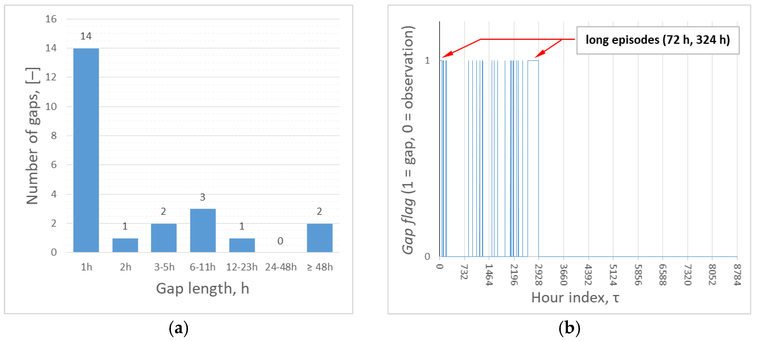
Figure 1. Statistical analysis of gaps in the hourly temperature series (ECO Opole, September 2019−August 2020): (a) Distribution of the length of consecutive gaps in the hourly temperature series (the numbers above the bars indicate the number of gaps in a given class). (b) Temporal distribution of gaps (vertical bars = hours without measurement; y-axis: gap flag, 1 = gap, 0 = observation). Two multi-day episodes (72 h, 324 h) are annotated; the remaining outages are short (≤6 h) and scattered throughout the season.
Energies 18 05547 g001
Figure 2. Actual outdoor temperature graph ta,obs(τ) for Opole from 1 September 2019 to 31 August 2020.
Energies 18 05547 g002
Figure 3. Block diagram with inputs/outputs and decision criteria (I–IV): normalization → ordered-domain fit ta,n → mapping back to time → KPI computation → lowest sufficient n.
Energies 18 05547 g003
Figure 4. Curves showing the duration of organized outdoor temperatures: a series of observations ta,obs, a reference series ta,ref (supplemented by AccuWeather), and a polynomial reconstruction ta,7 (n = 7). The table illustrates the consistency of the reconstruction with the reference throughout the season, including in areas with the highest heating loads.
Energies 18 05547 g004
Figure 5. ASHP design parameters for the heat-sink temperatures analyzed: (a) electrical power requirement; (b) COP.
Energies 18 05547 g005
Figure 6. The annual heat demand load duration curve for the 2019–2020 season for the analyzed building.
Energies 18 05547 g006
Figure 7. Comparison of demand and source capacity: curve of the duration of the building’s heat demand Q ˙ h , s h τ z compared with the maximum heating capacity of ASHP Q ˙ h , H P τ and the corresponding electrical power Pel(τ) dla LWT = {35, 45} °C (season 2019–2020, ta,ref). Areas where Q ˙ h , H P τ < Q ˙ h , s h τ indicate a bivalent point. In the analyzed year, no bivalence occurred; peak-power errors reflect only reconstruction and map effects.
Energies 18 05547 g007
Table 1. Constant a, b (in Equation (7)) of exponential approximations for Pel and COP, selected ASHP model, in two LWT regimes.
Return Water Temperature LWT PelCOP
Constants of Function
°Cabab
353.2097324−0.00412143.35598480.0266827
453.74262510.00049452.74139440.0230053
Table 2. Features of the tested building.
Building ParameterSymbolValueUnit
Peak heat demand of the building Q ˙ h , m a x 12.72kW
Temperature-controlled usable areaAf250m2
Normal operating (service) temperatureti21°C
Number of people residing in the facilityLi6j.o.
Individual daily hot water consumptionVcw50dm3/person/day
Hot water mode (average hourly power) Q ˙ h , h t w 0.65kW
Design outdoor temperature, climate zone IIIta,min−20°C
Seasonal outdoor temperature limitta,bs12°C
Table 3. Peak heat demand Q ˙ h , s h _ m a x , r e f and seasonal deviation of usable energy ΔQseason in the function of degree n. Reference and reconstructed values and the absolute (Δ) and relative difference (RE) are presented.
n Q ˙ h , s h _ m a x , r e f Q ˙ h , s h _ m a x , n Q ˙ h , s h , m a x R E Q ˙ h , s h , m a x Q s e a s o n R E Q s e a s o n
kWkWkW%kWh%
37.7426.885−0.858−11.08−367.3−1.64
47.7426.683−1.059−13.68−403.8−1.81
57.7427.189−0.553−7.15−291.2−1.30
67.7427.086−0.656−8.47−276.5−1.24
77.7427.264−0.479−6.18−296.4−1.33
87.7427.251−0.491−6.35−297.9−1.33
97.7427.386−0.357−4.61−290.4−1.30
107.7427.354−0.388−5.02−286.8−1.28
117.7427.332−0.410−5.30−284.9−1.27
Note: positive RE = overestimation relative to the reference; negative RE = underestimation.
Table 4. ASHP energy indicators are a degree n function for two LWT regimes; Δ values are absolute; RE values are relative (Equations (14)–(16)).
LWTnΔEel R E E e l ΔPel,max R E P e l , m a x ΔSCOP R E S C O P ΔCOPmin R E C O P m i n
°C kWh%kW%[-]%[-]%
353−123.0−2.07−0.471−17.730.02790.710.23558.08
4−131.7−2.22−0.574−21.590.03130.800.293610.08
5−97.3−1.64−0.311−11.690.02220.570.14995.14
6−94.4−1.59−0.366−13.760.02080.530.17856.13
7−99.8−1.68−0.270−10.170.02250.580.12924.44
8−100.2−1.69−0.277−10.420.02260.580.13274.55
9−97.8−1.65−0.203−7.650.02200.560.09583.29
10−96.9−1.63−0.221−8.300.02170.560.10443.58
11−96.5−1.63−0.233−8.760.02150.550.11043.79
453−7.2−0.44−0.017−6.480.01480.410.16826.93
4−7.2−0.44−0.021−7.950.01500.420.20958.63
5−7.1−0.43−0.011−4.230.01530.420.10734.42
6−7.1−0.43−0.013−5.000.01530.430.12765.26
7−7.1−0.43−0.010−3.670.01530.430.09253.81
8−7.1−0.43−0.010−3.770.01530.430.09503.91
9−7.1−0.43−0.007−2.750.01540.430.06862.83
10−7.1−0.43−0.008−2.990.01540.430.07483.08
11−7.1−0.43−0.008−3.160.01540.430.07913.26
Table 5. Fulfilment of the conditions for selecting the “lowest sufficient” degree n according to Criteria I-IV: “✓“ fulfilled, “△“ on the borderline, “—“ not fulfilled.
nCriteria
IIIIIIIV
3
4
5
6
7
8
9
10
11
Disclaimer/Publisher’s Note: The statements, opinions and data contained in all publications are solely those of the individual author(s) and contributor(s) and not of MDPI and/or the editor(s). MDPI and/or the editor(s) disclaim responsibility for any injury to people or property resulting from any ideas, methods, instructions or products referred to in the content.