CBATE-Net: An Accurate Battery Capacity and State-of-Health (SoH) Estimation Tool for Energy Storage Systems

Abstract

In battery energy storage systems, accurately estimating battery capacity and state of health is crucial to ensure satisfactory operation and system efficiency and reliability. However, these tasks present particular challenges under irregular charge–discharge conditions, such as those encountered in renewable energy integration and electric vehicles, where heterogeneous cycling accelerates degradation. This study introduces a hybrid deep learning framework to address these challenges. It combines convolutional layers for localized feature extraction, bidirectional recurrent units for sequential learning and a temporal attention mechanism. The proposed hybrid deep learning model, termed CBATE-Net, uses ensemble averaging to improve stability and emphasizes degradation-critical intervals. The framework was evaluated using voltage, current and temperature signals from four benchmark lithium-ion cells across complete life cycles, as part of the NASA dataset. The results demonstrate that the proposed method can accurately track both smooth and abrupt capacity fade while maintaining stability near the end of the life cycle, an area in which conventional models often struggle. Integrating feature learning, temporal modelling and robustness enhancements in a unified design provides the framework with the ability to make accurate and interpretable predictions, making it suitable for deployment in real-world battery energy storage applications.

1. Introduction

Lithium-ion batteries are the best choice for today’s electric vehicles (EVs), portable gadgets and renewable energy systems (RESs) because they are highly energy-dense, long-lasting, and quick to charge [1,2,3]. They play an extremely important role in large-scale energy storage systems (ESSs), distributed grids (DGs) and photovoltaic (PV) applications. For example, in an on-board ESS, they buffer intermittent solar generation and stabilize power delivery [4,5,6]. The growing reliance on lithium-ion batteries is reflected in the projected increase in global demand, which is expected to rise from 225 GWh in 2021 to nearly 815 GWh by 2025 [7]. The transportation sector is set to represent the largest share of this demand, as illustrated in Figure 1. This rapid expansion highlights the importance of ensuring that batteries operate safely, efficiently and reliably throughout their service life.

1.1. Background Study

A key parameter in assessing battery health is capacity, which is defined as the maximum charge that a cell can store and deliver under specific conditions [8]. Degradation of capacity directly defines state of health (SoH) and determines remaining useful life (RUL), which is typically marked at 1.40 Ah of the rated capacity [9]. Therefore, accurate capacity estimation is essential not only for performance forecasting, but also for safety and maintenance scheduling [10].

Over the past decade, several methods have been pursued.

• Experimental and model-based methods rely on open-circuit voltage (OCV), full charge–discharge cycles and electrochemical impedance spectroscopy (EIS) [11,12,13]. While these methods provide accurate battery capacity and state of health (SoH) estimation, they are costly, intrusive and unsuitable for continuous field monitoring [14]. Electrochemical models (EMs) capture detailed dynamics but require solving complex nonlinear equations, which limits their real-time applicability [15]. Furthermore, equivalent circuit models (ECMs) approximate behavior using lumped parameters but demand frequent recalibration [16,17].
• Data-driven methods learn from routine telemetry of voltage, current, and temperature of lithium-ion battery cells [18]. Classical regressors, such as support vector regression (SVR), random forest (RF), and Gaussian process regression (GPR), capture nonlinear degradation when provided informative features [19,20]. Deep learning (DL) models extends this by automatically extracting patterns. In these models, convolutional neural networks (CNNs) capture localized temporal cues, long short-term memory (LSTM) and bidirectional long short-term memory (BiLSTM) model sequential dependencies [21,22,23], and transformers use self-attention to represent long-range relations [24]. Hybrid CNN-Transformer designs integrate local and global contexts [22]. Their main strength lies in adaptability and real-time deployment once trained, but performance strongly depends on dataset quality, preprocessing, and robustness strategies [25,26].

While these developments show clear progress, challenges remain. Both experimental and model-based methods face issues of scalability and computational cost. Although data-driven approaches are more flexible, they require architectures capable of generalizing across irregular and heterogeneous degradation patterns, which are often observed in real-world systems.

1.2. Novelty and Motivation

The growing dependence on lithium-ion batteries in EV, RES, aviation, and industrial systems makes accurate capacity and SoH estimation a safety-critical and performance-critical task. Failures in battery management systems (BMSs) can result in severe incidents ranging from unexpected shutdowns to catastrophic thermal events.

Table 1. Real accident cases linked to battery management faults across domains.

Domain	Year	Incident	Cause
Automotive	2011	Chevrolet Volt delayed fire post-crash	Damaged battery thermal failure
Automotive	2011	Zotye M300 EV taxi fire (The manufacturer was Zotye, a company based in Zhejiang, China, and the fire occurred with a taxi in Hangzhou, China).	Battery pack defects (leaks, insulation failure)
Aviation	2013	Boeing 787 battery fires and grounding (GS Yuasa, a manufacturer based in Kyoto, Japan).	Internal short circuits, thermal runaway in BMS
Workshop/Transit	2021–2022	Street Scooter workshop fire; electric bus/ferry fires	Faulty batteries in EVs and energy systems
Maritime	2023	MV Fremantle Highway fire	Suspected EV battery ignition during transport
Industrial	2024	Hwaseong factory explosion/fire	Battery explosions in large-scale storage

presents case studies of accidents that have occurred in the automotive, aviation, maritime and industrial sectors. These real-world examples of failure demonstrate that battery capacity and state of health (SoH) estimation must be considered not only as diagnostic tools, but also as essential safeguards for ensuring safety, reliability and cost-effective operation.

Figure 2 shows the broader concept of prognostics and health management (PHM). Although PHM principles apply to various subsystems, including PV panels, power electronics and different types of load, the battery is the most dynamic and degradation-prone component. Its health directly influences the stability of the entire system. Therefore, accurate estimation of battery capacity and SoH sits at the core of PHM for battery energy storage systems (BESSs).

Despite advances in experimental, model-based, and data-driven methods, many challenges remain. Experimental and model-based approaches, while interpretable, are intrusive, computationally intensive, and unsuitable for real-time use. Data-driven methods and hybrid neural networks, on the other hand, show strong potential, but often lack robustness under heterogeneous cycling and noisy field conditions.

The novelty of this work lies in addressing these gaps through CNN-BiLSTM with Temporal Attention and Ensemble network (CBATE-Net). It is a hybrid DL framework that integrates CNN for localized feature extraction, BiLSTM for sequential modeling, temporal attention for selective weighting of degradation-relevant intervals, and ensemble learning for stability. This combination enables accurate and interpretable battery capacity and SoH estimation under irregular operating conditions, including PV-coupled applications, where variability in solar generation and load demand accelerates degradation.

To situate these contributions clearly, the next section outlines the main research contributions and the overall organization of this paper.

Figure 2. An illustration of PHM for aging estimation [27].

Figure 2. An illustration of PHM for aging estimation [27].

1.3. Contributions and Organization

The main contributions of this study are summarized as follows:

• Utilize the NASA Prognostics Center of Excellence (PCoE) lithium-ion batteries dataset. The operating specifications of each battery are summarized in Table 2.
• Develop a hybrid prognostic framework (CBATE-Net): A unified architecture that integrates convolutional neural networks for local feature extraction, bidirectional long short-term memory networks (BiLSTM) for sequence modeling, temporal attention for selective focus on degradation-relevant intervals, and ensemble learning as shown in Table 3 for robust predictions.
• Establish a standardized preprocessing pipeline: Discharge signals from the NASA PCoE lithium-ion batteries dataset [26] are aligned, resampled, cleaned, and normalized to produce cycle-wise sequences suitable for deep learning.
• Construct and analyze a 12-dimensional feature set: Features derived from voltage, current, and temperature signals along with their derivatives and energy descriptors are evaluated for correlation with capacity and SoH to ensure statistical relevance.
• Demonstrate robustness across heterogeneous cycling: The framework is evaluated on four NASA cells with distinct degradation trajectories, confirming its adaptability under irregular and noisy operating conditions.
• Provide interpretability through temporal attention and ablation analysis: The attention mechanism highlights critical intervals of discharge profiles, while ablation studies quantify the contribution of each model component.
• Position the framework for deployment in real-world applications: The model supports accurate, interpretable, and stable predictions for capacity and SoH, making it suitable for safety-critical domains, such as in EV, grid-level storage, and PV-coupled energy systems.

Many studies combine convolution, bidirectional LSTM, and attention for SoH or capacity. Our work contributes (i) an ensemble-integrated hybrid defined as part of the model with ablation studies and per seed reporting that show variance reduction and improved stability near end-of-life; (ii) a deployment profile in Table 4 that reports parameter count, compute, latency, and memory supporting embedded BMS feasibility; (iii) time-aware evaluation made primary with strictly time-forward protocols in Section 4.1 and results summarized in Table 5 and Table 6; (iv) a unified training and evaluation pipeline with a single feature set and identical preprocessing and splits for all methods so the comparisons in Table 6 and Table 7 are strictly comparable; finally, (v) a decision-level remaining useful life definition tied to the dataset’s end-of-life rule in Section 4.3.

The aim of this study is organized as follows. Section 2 reviews related works. Section 3 presents the adopted framework, NASA PCoE dataset of lithium-ion batteries, data preprocessing, feature extraction steps, the proposed CBATE-Net architecture, and the training and model selection procedure. Section 4 reports experimental results, discusses error dynamics and ensemble stability, and RUL estimation from capacity predictions. Section 5 compares the framework with conventional machine learning (ML), deep learning (DL), and transformer-based models. Section 6 presents ablation studies, and Section 7 concludes the paper with future research directions.

In summary, this work contributes a robust and interpretable framework for battery capacity and SoH estimation, offering a practical step toward safer and more reliable BESS under diverse and irregular operating conditions.

2. Related Works

2.1. Overview of Capacity and SoH

Battery capacity quantifies the maximum charge a cell can store and deliver under specified conditions. It is computed as the integral of discharge current over time

$$C={\int }_{t_0}^{t_f}I\left(t\right)dt$$

(1)

where $I\left(t\right)$ is the discharge current, and $t_0$ and $t_f$ denote the start and end of discharge. In an ESS, with repeated cycling, capacity decreases due to electrochemical and mechanical degradation. The state of SoH provides a normalized measure of this degradation and is commonly expressed as

$$\mathrm{SoH}={\displaystyle \frac{C_{\mathrm{measured}}}{C_{\mathrm{rated}}}}\times 100\%.$$

(2)

Here $C_{\mathrm{measured}}$ is the measured capacity from a given cycle and $C_{\mathrm{rated}}$ is the nominal rated capacity. This definition makes capacity estimation the direct basis for SoH inference. When combined with the end-of-life threshold used in this study, defined as capacity ≤ 1.40 Ah according to the NASA PCoE protocol, the SoH-based RUL estimation becomes well defined. For the four cells analyzed, this threshold corresponds to approximately 70 percent of the rated capacity. Accurate prediction of battery capacity and SoH is therefore essential for reliable operation of BESS, especially under irregular charge–discharge conditions, where degradation paths are heterogeneous.

2.2. Existing Approaches

Existing approaches for battery capacity and SoH estimation can be grouped into experimental and model-based, feature-driven ML, DL, hybrid, and transformer-based methods.

Experimental and model-based methods rely on EM, ECM, and analysis-based techniques, such as incremental capacity (IC), differential voltage, and EIS [28,29,30]. These provide accurate degradation insight, but require repeated parameter identification, complex solvers, or intrusive measurements, making them unsuitable for continuous onboard monitoring [31].

Feature-driven ML methods map handcrafted features, such as partial charging time (PCT) or multi-channel charging profiles (MCCPs) for capacity estimation. Classical regressors including SVR, RF, and boosting methods have been applied [32,33]. While interpretable, their performance depends on feature design and dataset-specific tuning.

DL methods reduce reliance on manual features by directly learning from voltage, current, and temperature signals. CNN capture localized patterns, LSTM and BiLSTM model temporal dependencies, and combined CNN-LSTM models have demonstrated improved accuracy over voltage-only inputs [27,34]. However, most studies were validated on limited datasets, restricting generalization.

Hybrid architectures integrate local and sequential modeling. Examples include CNN-BiLSTM hybrids and neural networks (NNs) augmented with impedance or wavelet-based indicators [16,35]. These models achieve high accuracy, but often rely on engineered health indicators (HIs), have heavy data preprocessing and limited scalability range.

Transformer-based models employ self-attention to capture long-range dependencies. CNN-Transformer hybrids and temperature-impedance fusion schemes have reported high accuracy on NASA PCoE datasets [8,36]. Robustness has been enhanced with augmentation strategies [37]. Despite their potential, transformers are computationally intensive and typically lack uncertainty calibration.

Finally, surveys and reviews highlight persistent gaps in dataset quality, preprocessing robustness, and generalization [28,31,38]. Collectively, these approaches show steady progress, but also reveal open challenges that motivate the hybrid framework developed in this study.

2.3. Challenges in Existing Approaches

Despite notable progress, there are still several gaps that limit the reliability of current methods for estimating battery capacity and state of health (SoH). Experimental and model-based approaches are still intrusive, time-consuming and computationally demanding, preventing real-time use. On the other hand, data-driven models rely heavily on dataset quality; however, variability in cycling conditions and environmental factors reduces their generalization [39]. Hand-crafted features only capture local cues, and pure sequential models may miss short but critical degradation events [40]. Transformer variants improve global context but require high computational resources, which makes embedded deployment difficult. Finally, most methods lack robustness mechanisms against noise and initialization, leading to unstable predictions near the end of the battery’s life. These open issues motivate a hybrid design combining localized feature extraction, temporal modelling, selective attention and ensemble stability to form the basis of the framework presented in the next section.

2.4. Technical Foundations of the Proposed Framework

Recent advances in battery prognostics combine spatial feature extraction, temporal modelling, attention and ensemble strategies. CNNs extract localized degradation cues from voltage, current and temperature sequences, capturing short-term variations linked to early aging [22]. BiLSTM then extends this by learning long-range dependencies in both the forward and backward directions, establishing links between the early and late stages of a lithium-ion battery discharge cycle [41]. A temporal attention mechanism highlights the most informative time steps, emphasizing degradation-relevant intervals while de-emphasizing less significant ones [24]. Ensemble learning aggregates the outputs of multiple trained models to improve robustness and reduce sensitivity to noise and initialization [37]. The NASA PCoE dataset remains the most widely used benchmark for such models. It provides voltage, current and temperature signals across the full life cycles of lithium-ion cells and offers diverse degradation trajectories, including gradual, abrupt and accelerated fade [16,32]. These channels are already available in BMS, making them practical for onboard estimation. Together, these elements form the basis of the hybrid framework proposed in this study. The design directly addresses the challenges of robustness, interpretability, and scalability identified in Section 2.3 by combining CNN, BiLSTM, temporal attention, and ensemble averaging.

3. Proposed Methodology

3.1. Framework

The proposed CBATE-Net is an advanced, hybrid deep learning (DL) framework designed for the accurate estimation of battery capacity and state of health (SoH). It combines four elements: CNN for localized feature extraction, BiLSTM for sequence modelling, a temporal attention mechanism for selective weighting of degradation-relevant intervals, and ensemble learning for robustness.

The pipeline follows a sequential yet integrated flow within the overall system. First, discharge signals of voltage, current and temperature are preprocessed and converted into standardized, cycle-wise sequences. A feature set derived from these signals is then passed to the hybrid DL model. CNN layers capture local variations, BiLSTM learns long-term dependencies in both directions and the attention mechanism highlights critical intervals linked to degradation of the lithium-ion batteries. To improve stability and precision, multiple model instances are trained independently and their predictions are aggregated through ensemble averaging.

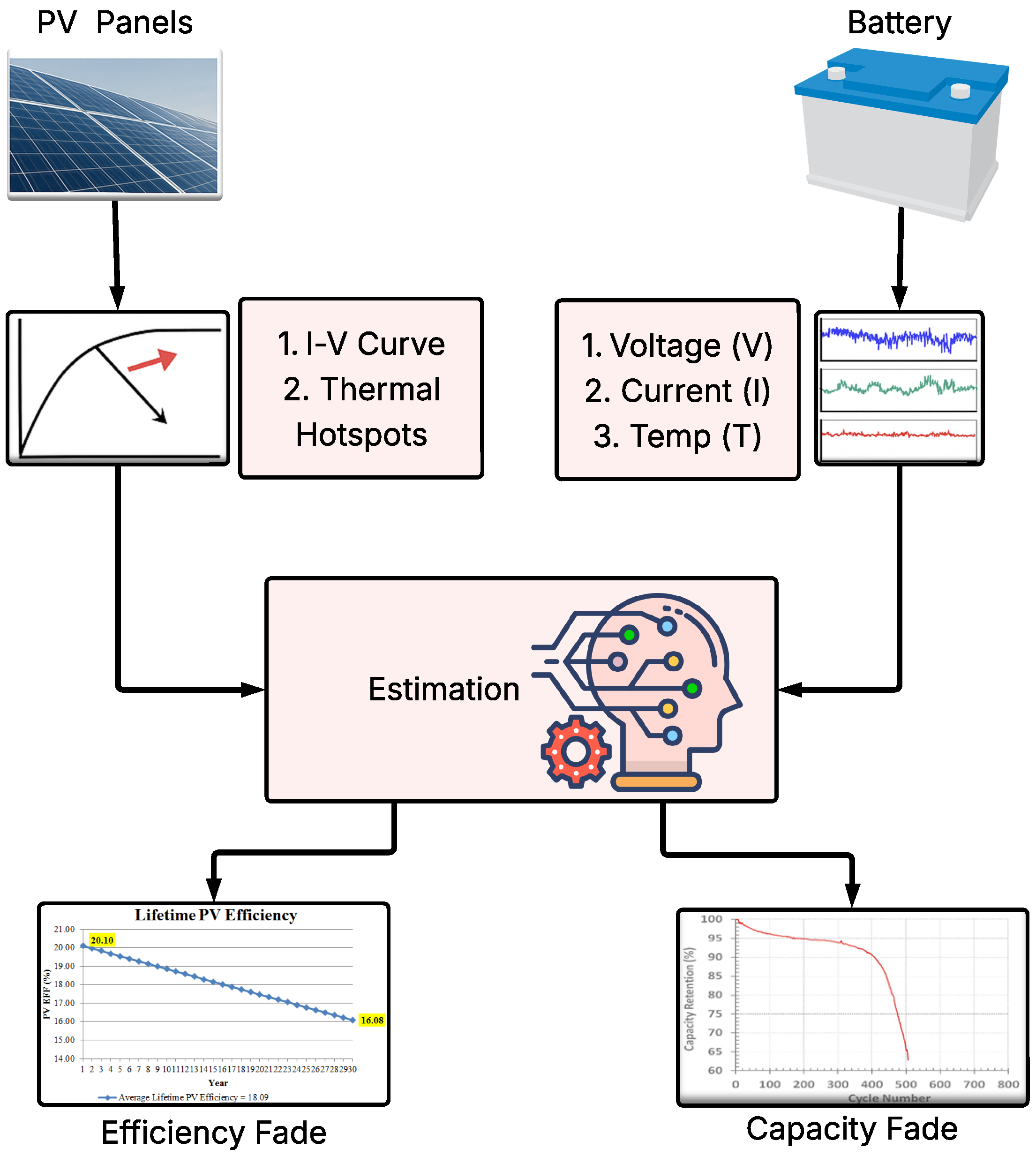
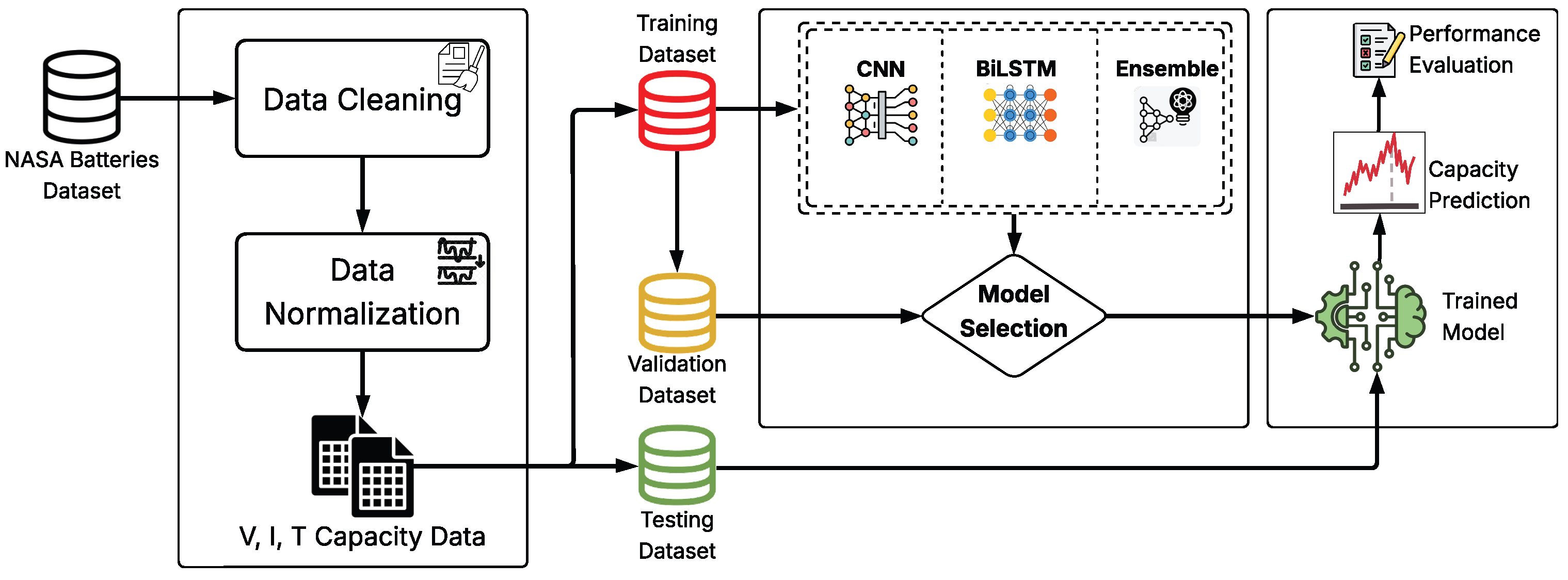
Figure 3 illustrates the workflow of the proposed framework. The pipeline begins with the NASA lithium-ion battery dataset, which is cleaned and normalized first. The processed voltage, current, and temperature signals are then divided into training, validation, and testing subsets. These data are passed through a hybrid DL model consisting of a CNN, a BiLSTM, and an ensemble module, after which model selection takes place. The final stage produces capacity predictions together with a performance evaluation. SoH can then be derived from the predicted capacity as the ratio of predicted to nominal capacity, and RUL can be estimated relative to the 1.40 Ah end-of-life threshold, as explained in later sections. This design captures both localized fluctuations and long-term degradation patterns, ensuring stable performance under irregular cycling conditions.

The input to the model consists of data with dimensions 256 by 12. This input is first passed through a one-dimensional convolutional layer with 32 filters and a kernel size of 5. The output is then normalized using batch normalization, followed by a ReLU activation function and a max-pooling layer with a pool size of 2. Next, the signal is processed by a second Conv1D layer containing 64 filters with a kernel size of 5, again followed by batch normalization, ReLU activation, and max-pooling with a size of 2.

A third Conv1D layer with 128 filters and a kernel size of 3 is then applied, followed by batch normalization, ReLU activation, and a dropout layer with a dropout probability of 0.10 to prevent overfitting. The extracted features are then fed into a sequence of three bidirectional LSTM layers; the first two have 128 units in each direction, and the final one has 64 units in each direction. After the recurrent layers, a temporal attention mechanism is applied to focus on the most relevant time steps in the sequence.

The attention-weighted output is then passed through a fully connected (dense) layer with 64 neurons, using the ReLU activation function and L2 regularization with a penalty coefficient of 1 × 10⁻⁴. The final layer is a single-neuron dense layer that produces the model’s output. The State of Health (SoH) is computed using Equation (2). Finally, to enhance robustness and accuracy, the final prediction is obtained by averaging the outputs of M independently trained models in an ensemble. Table 3 describes the complete layer-by-layer configuration for the complete architecture of the system.

3.2. Experimental Dataset of Lithium-Ion Batteries of NASA

This study uses the NASA lithium-ion battery dataset, which is widely adopted in the literature for battery capacity and state of health (SoH) evaluation [21,26]. The operating specifications of each battery are summarized in Table 2. Constant current (CC)–constant voltage (CV) charging occurs at 1.5 A to 4.2 V with a cut-off current of 20 mA. Similarly, the following cut-off voltages were obtained: 2.7 V (B0005), 2.5 V (B0006 and B0018) and 2.2 V (B0007). Furthermore, the initial capacity was found to range from 1.86 to 2.04 Ah, with an end-of-life threshold of 1.40 Ah. 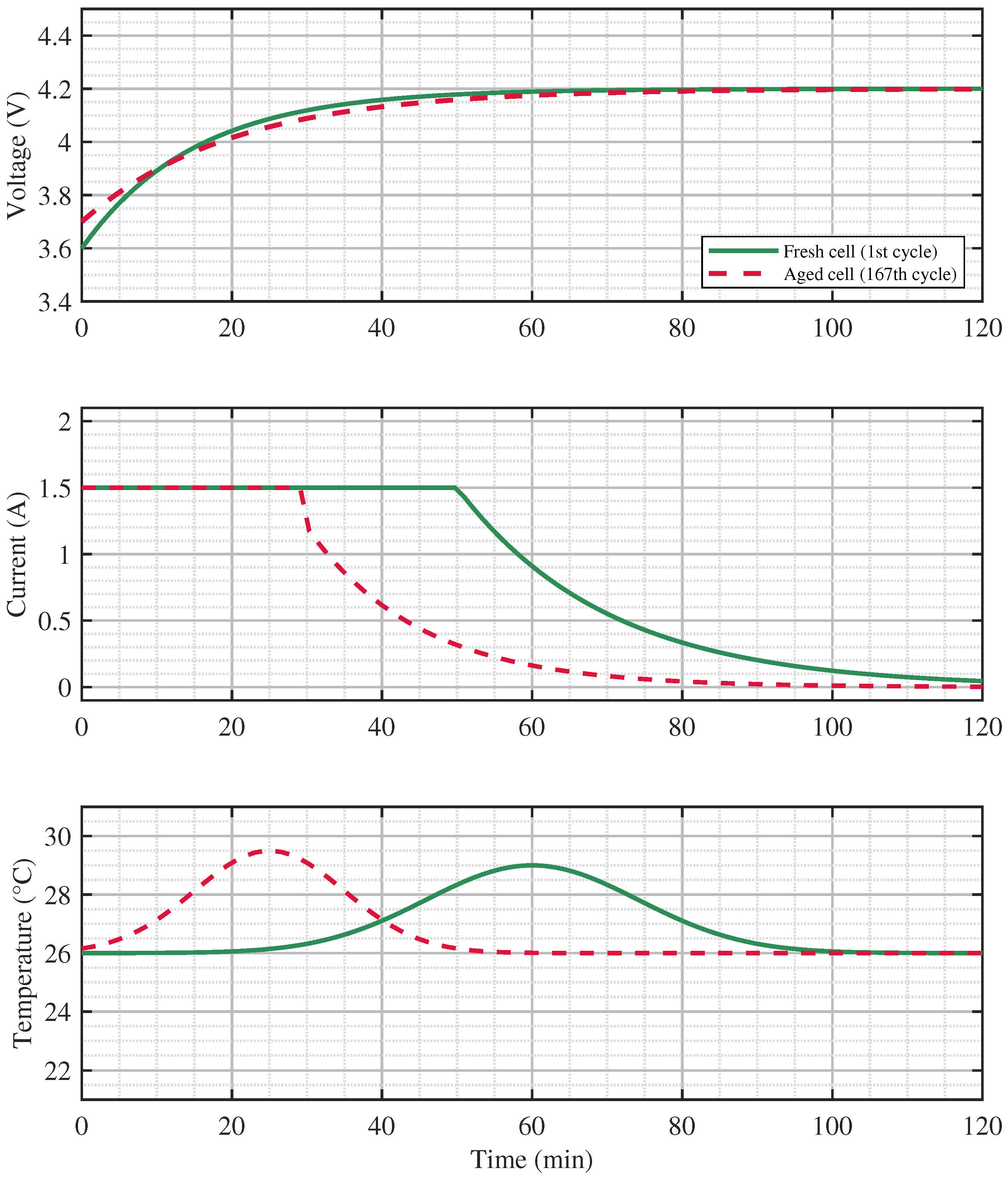Figure 4 shows the differences between the fresh and aged cycles of the lithium-ion battery parameters, such as voltage, current, and temperature over time in minutes. As the battery ages, there will be an early current discharge and temperature rise. Also, its output voltage decreases in amplitude. Therefore, the traces clearly show shifts in these parameters with usage and time.

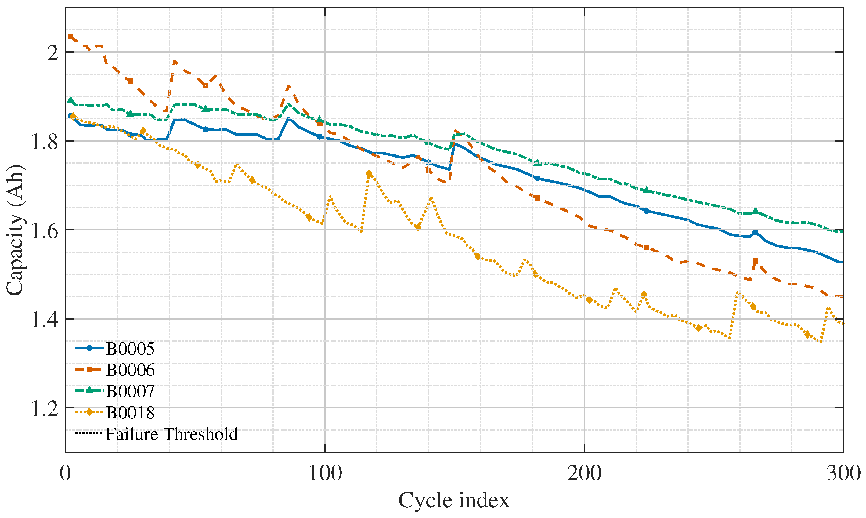
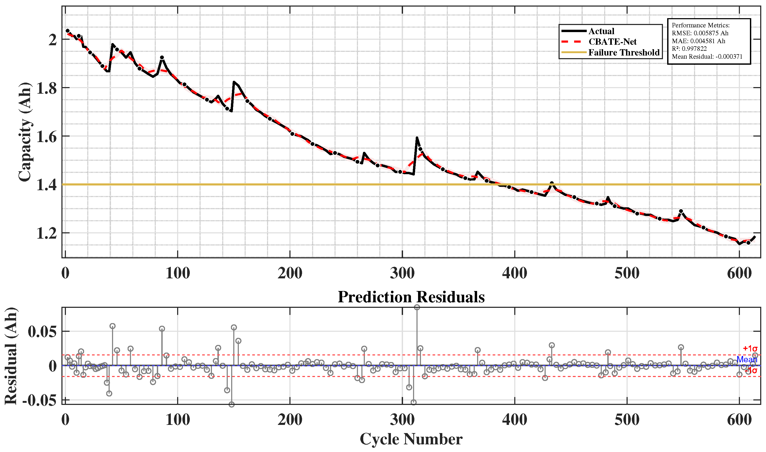
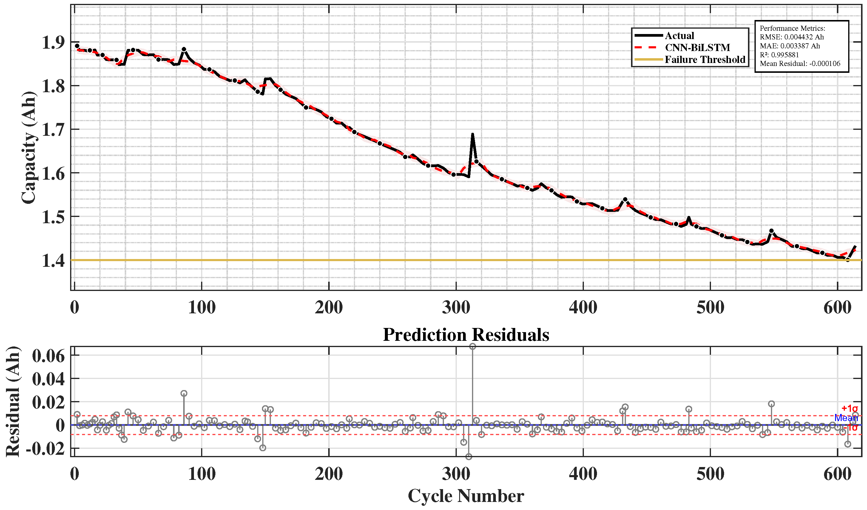
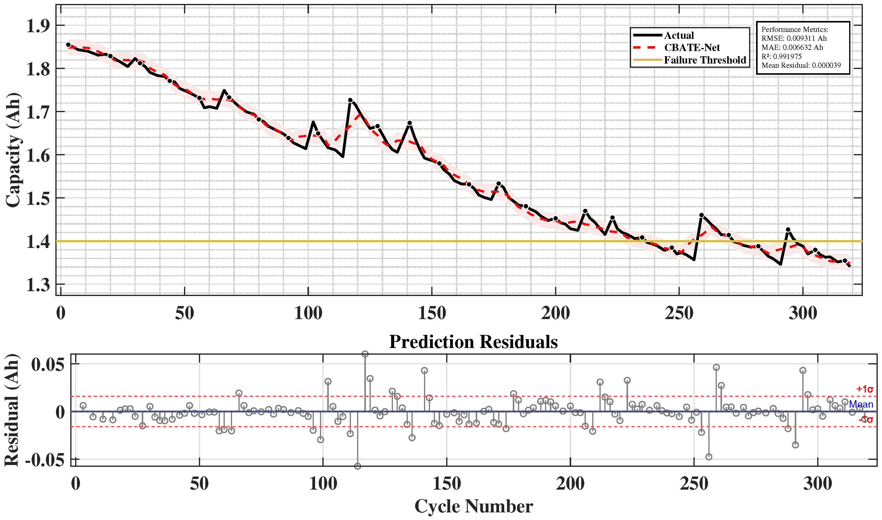
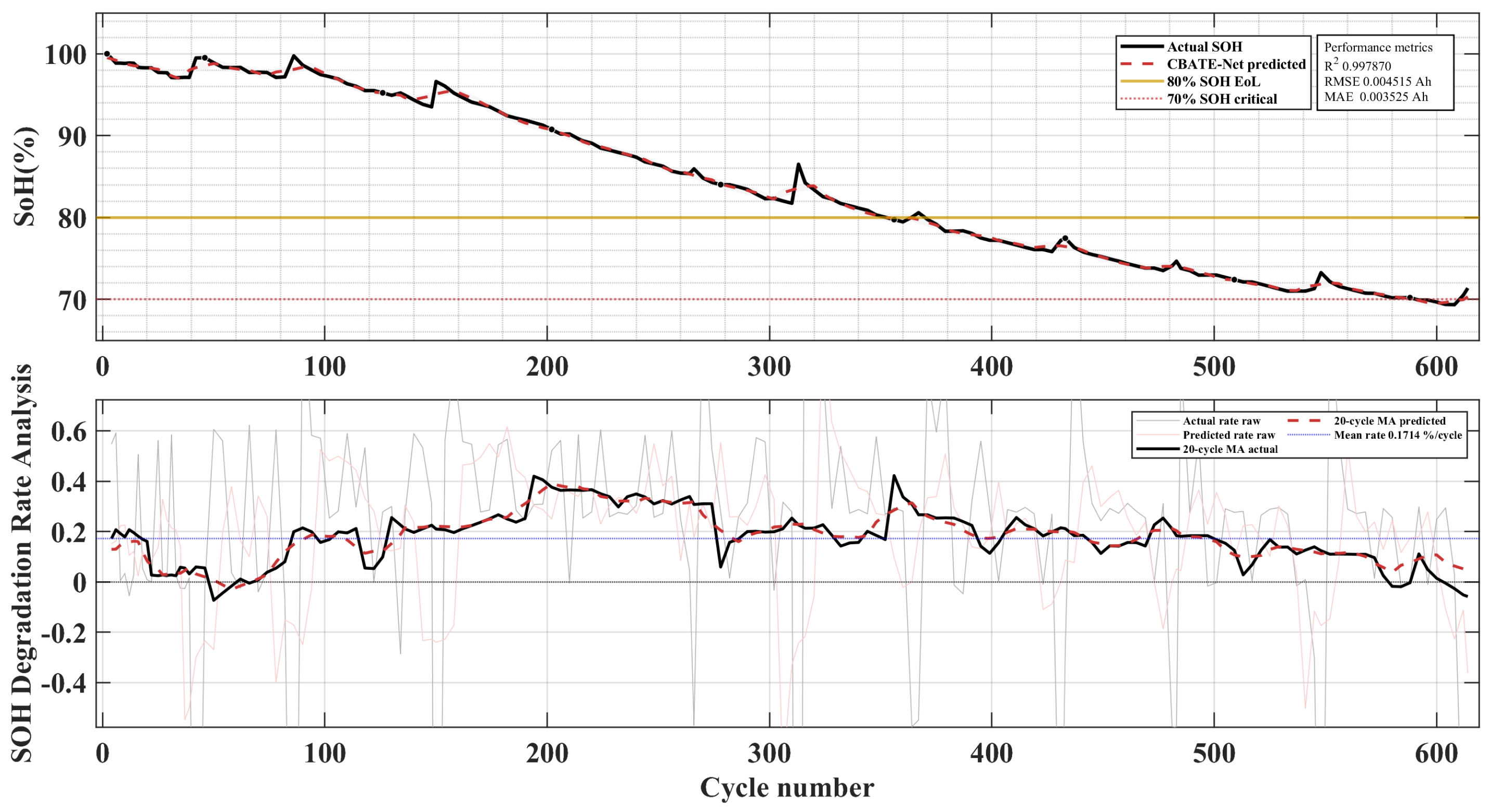
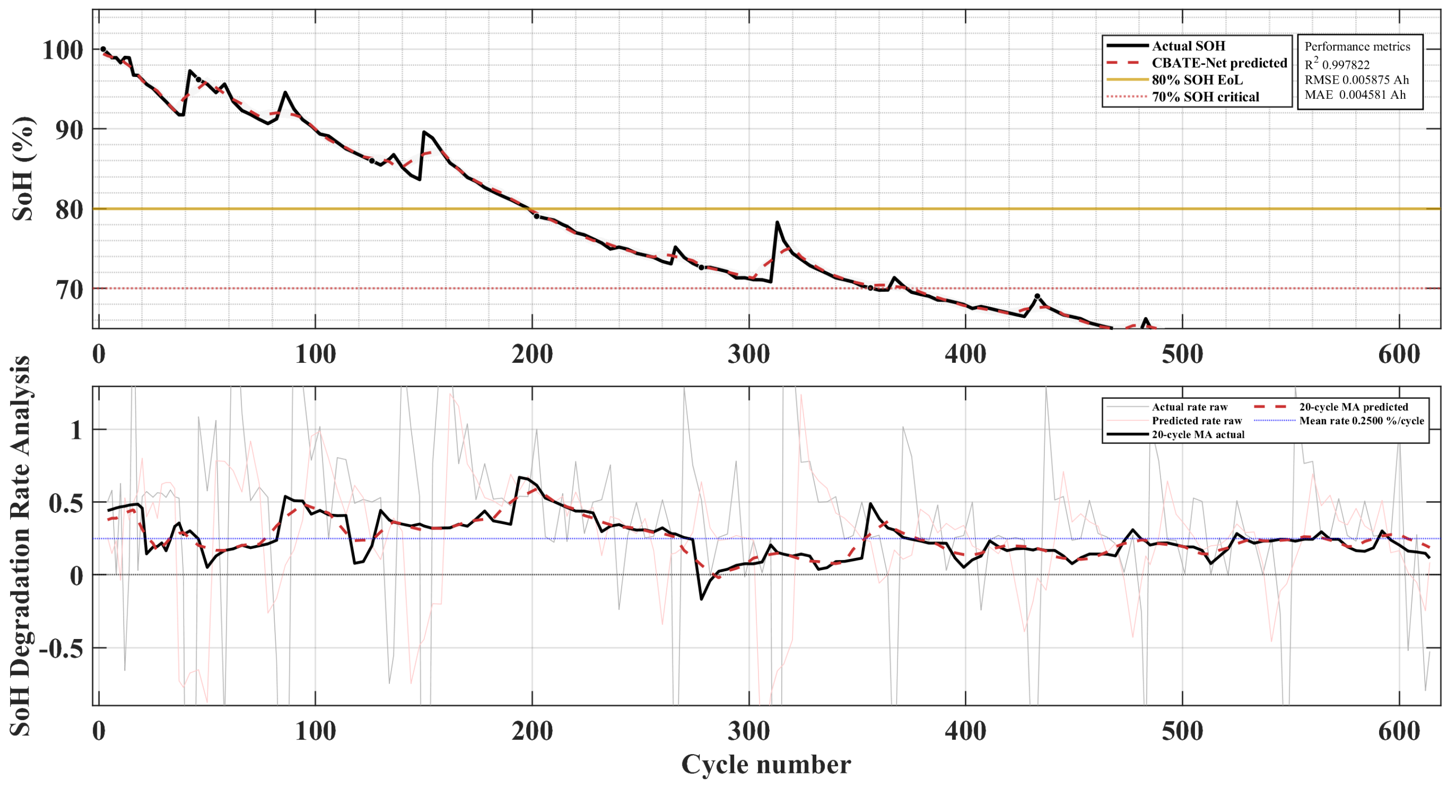
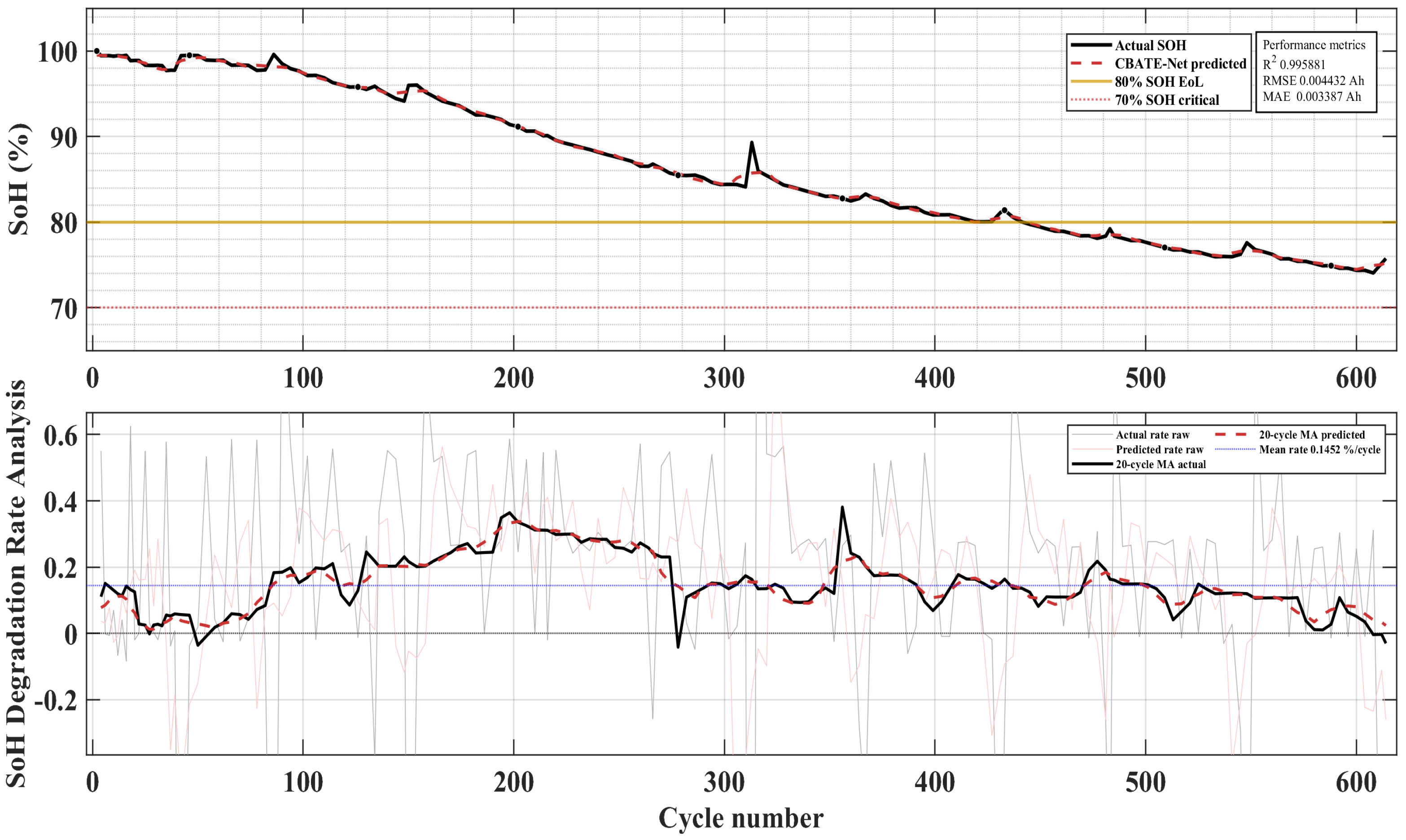
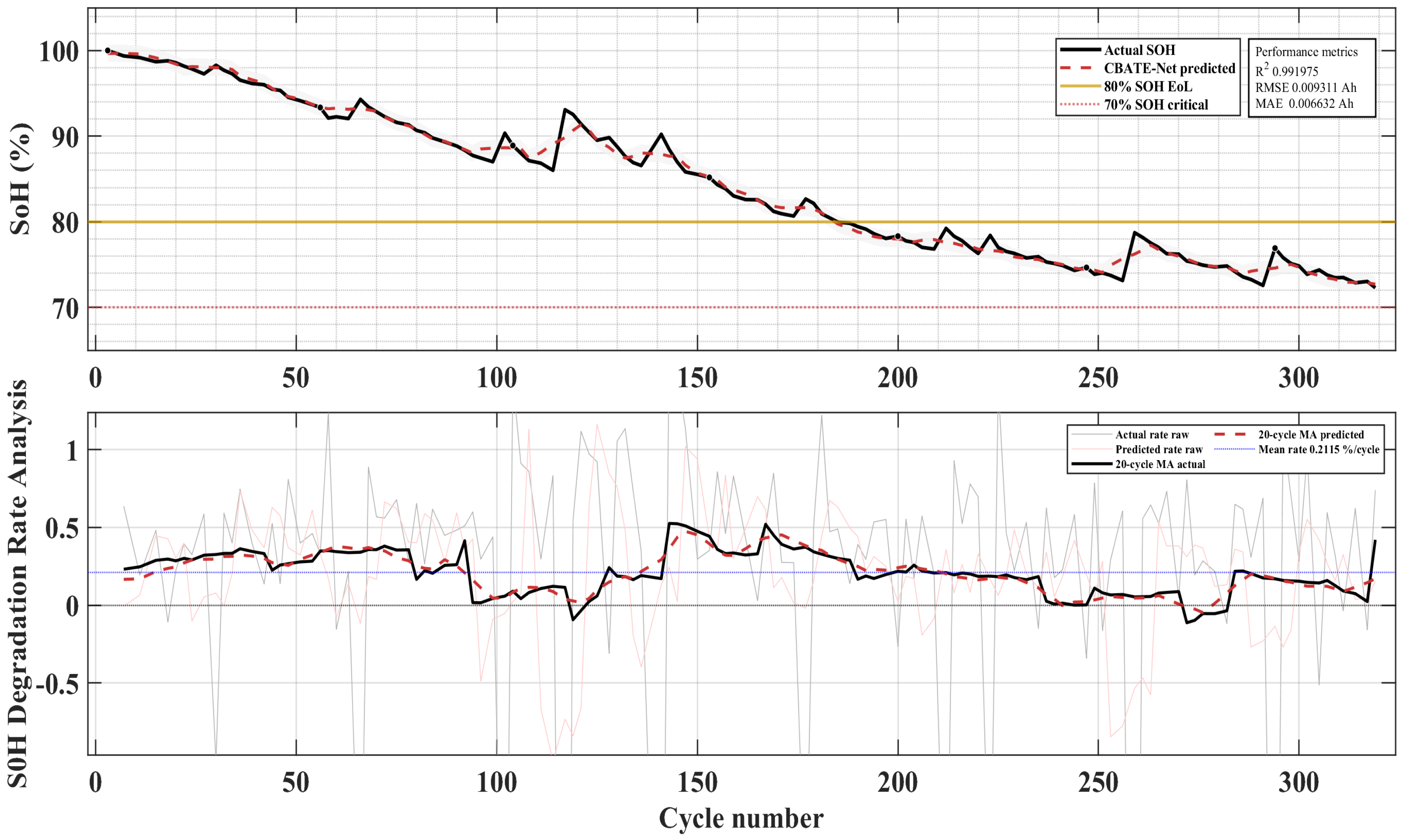
The corresponding battery capacity degradation trajectories are shown in Figure 5. These plots illustrate the diversity of aging behaviors: B0005 exhibits relatively regular degradation, B0006 demonstrates slightly higher capacity retention, B0007 suffers sudden early degradation, and B0018 shows accelerated capacity fade. This diversity provides a challenging and representative testbed for evaluating model robustness.

Table 2. Specifications of NASA lithium-ion batteries used in this study.

Battery ID	Charging Protocol (CC–CV)	Discharge Current (A)	Discharge Cut-Off Voltage (V)	Operating Temperature (°C)	Initial Capacity (Ah)	End-of-Life Criterion (Ah)	Role
B0005	1.5 A, 4.2 V, 20 mA cut-off	2.0	2.7	25 ± 2	1.86	1.40	Train/Test
B0006	1.5 A, 4.2 V, 20 mA cut-off	2.0	2.5	25 ± 2	2.04	1.40	Train/Test
B0007	1.5 A, 4.2 V, 20 mA cut-off	2.0	2.2	25 ± 2	1.89	1.40	Train/Test
B0018	1.5 A, 4.2 V, 20 mA cut-off	2.0	2.5	25 ± 2	1.86	1.40	Train/Test

Table 2. Specifications of NASA lithium-ion batteries used in this study.

Battery ID	Charging Protocol (CC–CV)	Discharge Current (A)	Discharge Cut-Off Voltage (V)	Operating Temperature (°C)	Initial Capacity (Ah)	End-of-Life Criterion (Ah)	Role
B0005	1.5 A, 4.2 V, 20 mA cut-off	2.0	2.7	25 ± 2	1.86	1.40	Train/Test
B0006	1.5 A, 4.2 V, 20 mA cut-off	2.0	2.5	25 ± 2	2.04	1.40	Train/Test
B0007	1.5 A, 4.2 V, 20 mA cut-off	2.0	2.2	25 ± 2	1.89	1.40	Train/Test
B0018	1.5 A, 4.2 V, 20 mA cut-off	2.0	2.5	25 ± 2	1.86	1.40	Train/Test

Figure 4. Time-series plots of voltage, current, and temperature for fresh (Cycle 1) and aged (Cycle 168) battery cells.

Figure 4. Time-series plots of voltage, current, and temperature for fresh (Cycle 1) and aged (Cycle 168) battery cells.

Figure 5. Capacity versus cycle number for NASA cells, with end of life threshold marked at 1.40 Ah, about 70 percent of nominal capacity.

Figure 5. Capacity versus cycle number for NASA cells, with end of life threshold marked at 1.40 Ah, about 70 percent of nominal capacity.

3.3. Data Preprocessing

Effective preprocessing is essential for converting raw discharge data into reliable training inputs. This study used multi-channel sequences of voltage, current, and temperature from four NASA PCoE lithium-ion cells (B0005, B0006, B0007 and B0018). Outlier cycles were removed using a median absolute deviation (MAD) filter and those with capacities outside the valid range of 0.5–2.5 Ah were excluded. After cleaning, all features were standardized by z-score normalization using training set statistics. For each channel j, the normalized value $x_j^{\left(n\right)}$ of a sample $a_j^{\left(n\right)}$ is computed as

$$x_j^{\left(n\right)}={\displaystyle \frac{a_j^{\left(n\right)}-{\mu }_j}{{\sigma }_j}},$$

(3)

where ${\mu }_j$ and ${\sigma }_j$ denote the mean and standard deviation of channel j in the training partition. Validation and test sets used the same parameters, and predictions were de-normalized after inference to recover their physical scale [42,43]. To improve generalization and avoid overfitting, light data augmentation was used only on the training set. Moreover, additive Gaussian noise was added with a mean of zero and a standard deviation of about 1–2 percent of each feature’s amplitude. Additionally, temporal jitter was also introduced, allowing a maximum shift of ±two sampling points, which is less than 0.5 percent of the total discharge time. These small changes simulate real sensor noise and slight timing errors found in actual BMS data. Therefore, the physical continuity of voltage, current, and temperature signals was preserved. Hence, no rescaling or artificial shape distortion was applied [18,44]. This reduced overfitting and improved generalization under irregular cycling conditions. 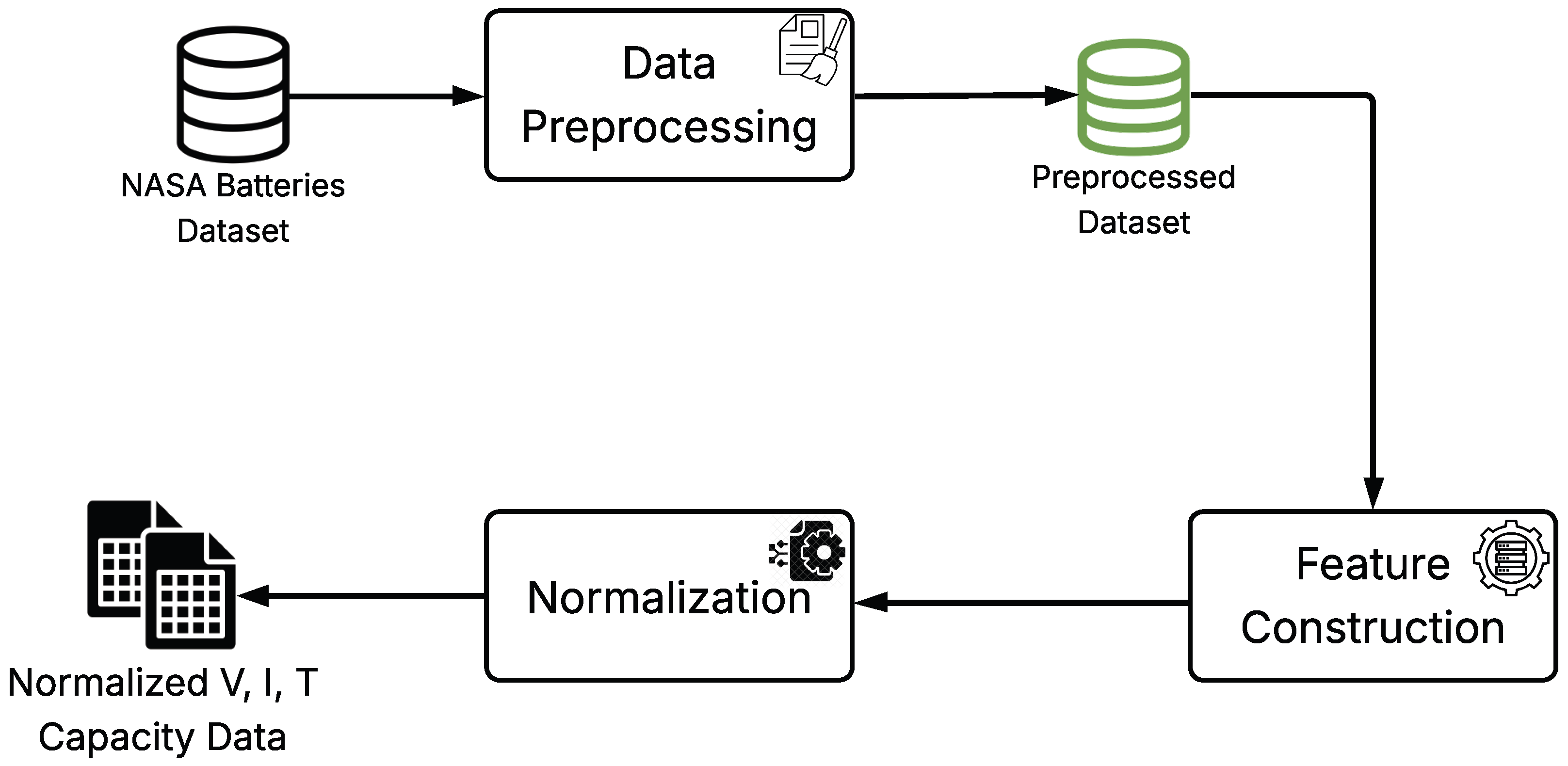Figure 6 shows the workflow of battery data processing and normalization.

3.4. Feature Extraction and Selection

Each discharge cycle was represented by a 12-dimensional feature vector derived from voltage, current, and temperature signals. The features included raw measurements (V, I, T), first- and second-order derivatives $\left(\mathrm{\Delta }V,\mathrm{\Delta }I,\mathrm{\Delta }T,{\mathrm{\Delta }}^{2}V,{\mathrm{\Delta }}^{2}I\right)$, power and energy terms $(P=V\times I,$ normalized cumulative E, smoothed moving averages, and discharge duration.

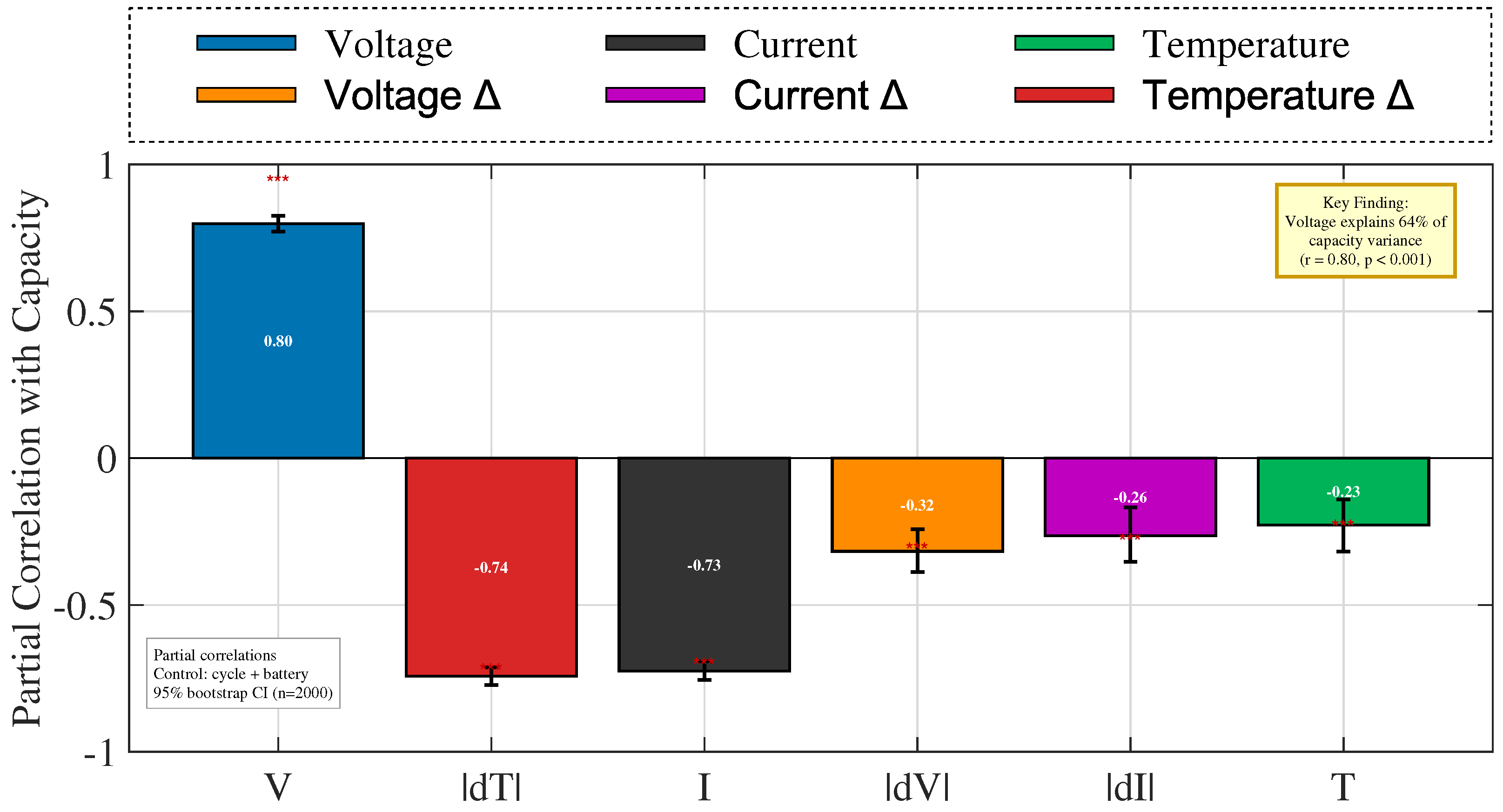
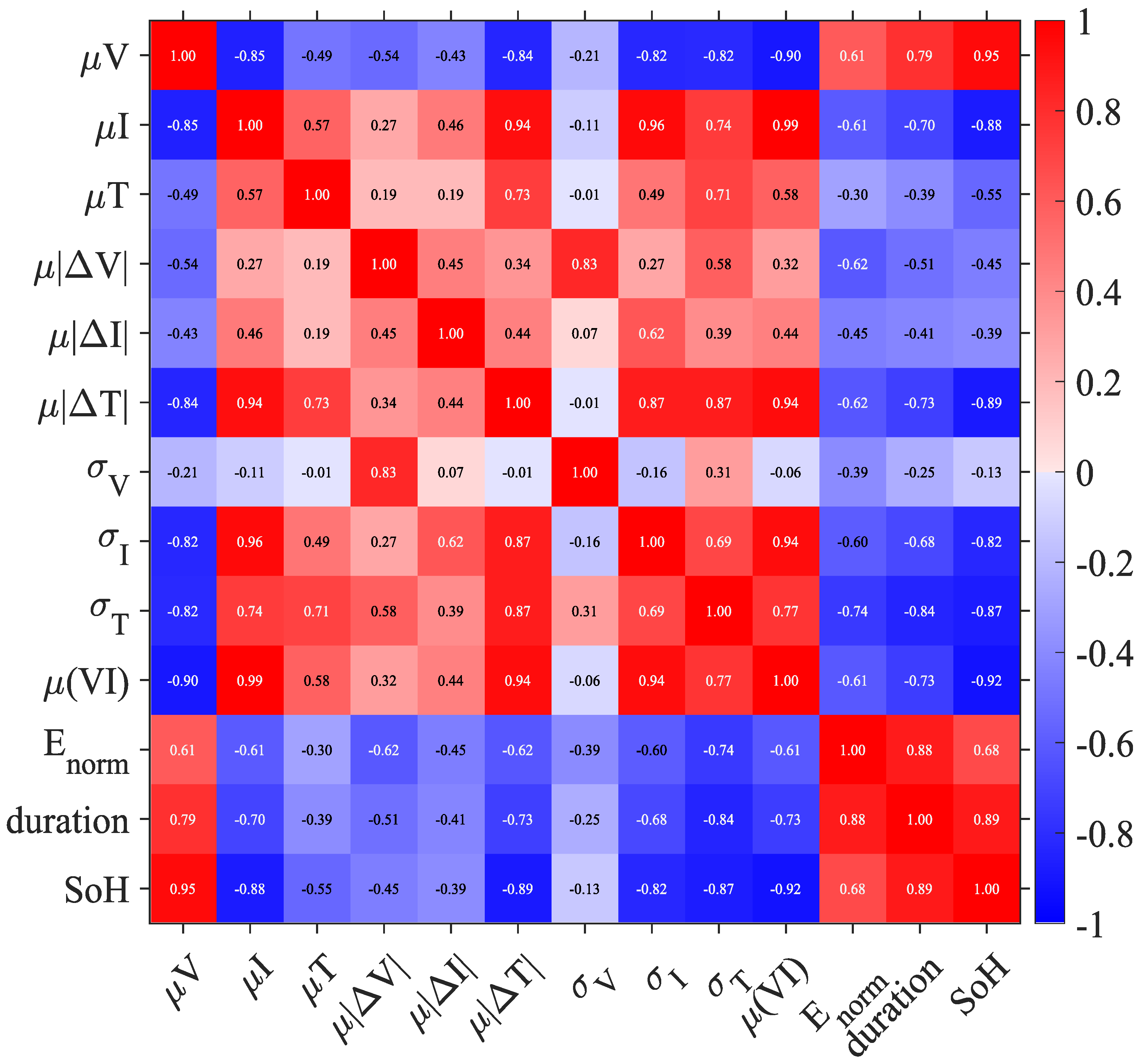
Figure 7 shows the z-score distributions of these features across cycles. Voltage and its derivatives display the highest variability, indicating high sensitivity to degradation, while temperature-related channels provide complementary thermal information. Figure 8 further reports partial correlation coefficients with measured capacity, controlling for cycle index and battery identity. Figure 9 presents the Pearson correlation matrix with SoH [45]. Both analyses confirm that multiple features are informative, and no single descriptor dominates degradation. Consequently, all features were retained as model inputs. This enables convolutional layers to emphasize localized signals and BiLSTM to capture temporal dependencies. Retaining all features allows CBATE-Net to exploit both strong predictors and complementary cues, preserving nonlinear interactions that might otherwise be lost.

3.5. CBATE-Net Models

Battery capacity and SoH estimation requires models that can capture short-term localized patterns and long-range sequential dependencies from multi-channel discharge data. Traditional regressors and handcrafted features are insufficient under heterogeneous operating conditions. Therefore, the proposed framework integrates four complementary components: CNN, BiLSTM networks, temporal attention, and ensemble learning. The following subsections (Section 3.5.1, Section 3.5.2, Section 3.5.3 and Section 3.5.4) describe each model family in detail and explain its role in the integrated CBATE-Net framework.

3.5.1. Convolutional Neural Network

CNN layers are employed at the feature extraction stage to capture short-term, localized patterns in the discharge signals of voltage (V), current (I), and surface temperature (T), which often indicate early degradation. Examples include slope changes in voltage or sudden temperature spikes, detected through convolutional filters. The convolution operation for a one-dimensional input sequence is:

$$r_t={\left(a\ast k\right)}_t=\sum _p{a}_{t-p}{k}_p,$$

(4)

where a is the input sequence (V, I, T), K is the kernel (learnable filter), and $r_t$ is the resulting feature at position t. The extracted features are then passed to the BiLSTM layers.

3.5.2. Bidirectional Long Short-Term Memory (BiLSTM)

While CNN layers effectively capture localized degradation patterns, accurate capacity and SoH prediction also requires modeling temporal dependencies that span the full discharge sequence. LSTM networks address this need through gated recurrent units that regulate information flow across time steps and mitigate vanishing or exploding gradients in conventional RNN [21,24,46,47]. In a standard LSTM, the memory cell $m_t$ is updated by balancing information from the previous state with new candidate input (using forget and input gates):

$$m_t=r_t·{\tilde{m}}_{t-1}+g_t·{\tilde{m}}_t,$$

(5)

where $r_t$ is the forget gate, $g_t$ is the input gate, and ${\tilde{m}}_t$ is the candidate update. The hidden states are updated as:

$$s_t=q_t·\mathrm{t}\mathrm{a}\mathrm{n}\mathrm{h}\left(m_t\right)$$

(6)

where $s_t$ is the hidden state (scaled by the output gate) and $q_t$ represents the output state. A Bidirectional LSTM (BiLSTM) extends this formulation by processing the sequence in both forward and backward directions, producing hidden states ${\mathbf{s}}_t^{\to }$ and ${\mathbf{s}}_t^{\leftarrow }$. The final representation is obtained by concatenating both directions:

$${\mathbf{s}}_t=\left[{\mathbf{s}}_t^{\to };{\mathbf{s}}_t^{\leftarrow }\right].$$

(7)

This bidirectional design enables the framework to jointly exploit early- and late-cycle degradation cues. The extracted features are then passed to the temporal attention model.

3.5.3. Temporal Attention

While BiLSTM layers capture sequential dependencies, they treat all time steps equally, which may reduce the influence of degradation-relevant segments in a discharge profile. To address this, a temporal attention mechanism assigns higher weights to critical time steps [48,49]. Given a sequence of hidden states ${\left\{h_t\right\}}_{t=1}^T$ produced by the BiLSTM, the attention weight ${\alpha }_t$ is computed as:

$${\alpha }_t={\displaystyle \frac{\mathrm{e}\mathrm{x}\mathrm{p}\left(e_t\right)}{{\sum }_{k=1}^T\mathrm{e}\mathrm{x}\mathrm{p}\left(e_t\right)}},e_t=f\left(h_t\right),$$

(8)

where $h_t$ is the hidden state at time step t, T is the total number of steps, $f\left(·\right)$ is a learnable scoring function, $e_t$ is the unnormalized importance score, $e_k$ is the normalization term, and ${\alpha }_t$ is the normalized attention weight with ${\sum }_{t=1}^T{\alpha }_t=1.$ The context vector is then obtained as a weighted sum of hidden states:

$$c=\sum _{t=1}^T{\alpha }_t{h}_t.$$

(9)

Here, c is the aggregated sequence representation that emphasizes intervals critical to degradation. This mechanism amplifies critical regions, such as voltage plateaus that flatten with aging or temperature segments with accelerated rise. By focusing on these subsequences, temporal attention improves both interpretability and predictive accuracy.

3.5.4. Ensemble Learning

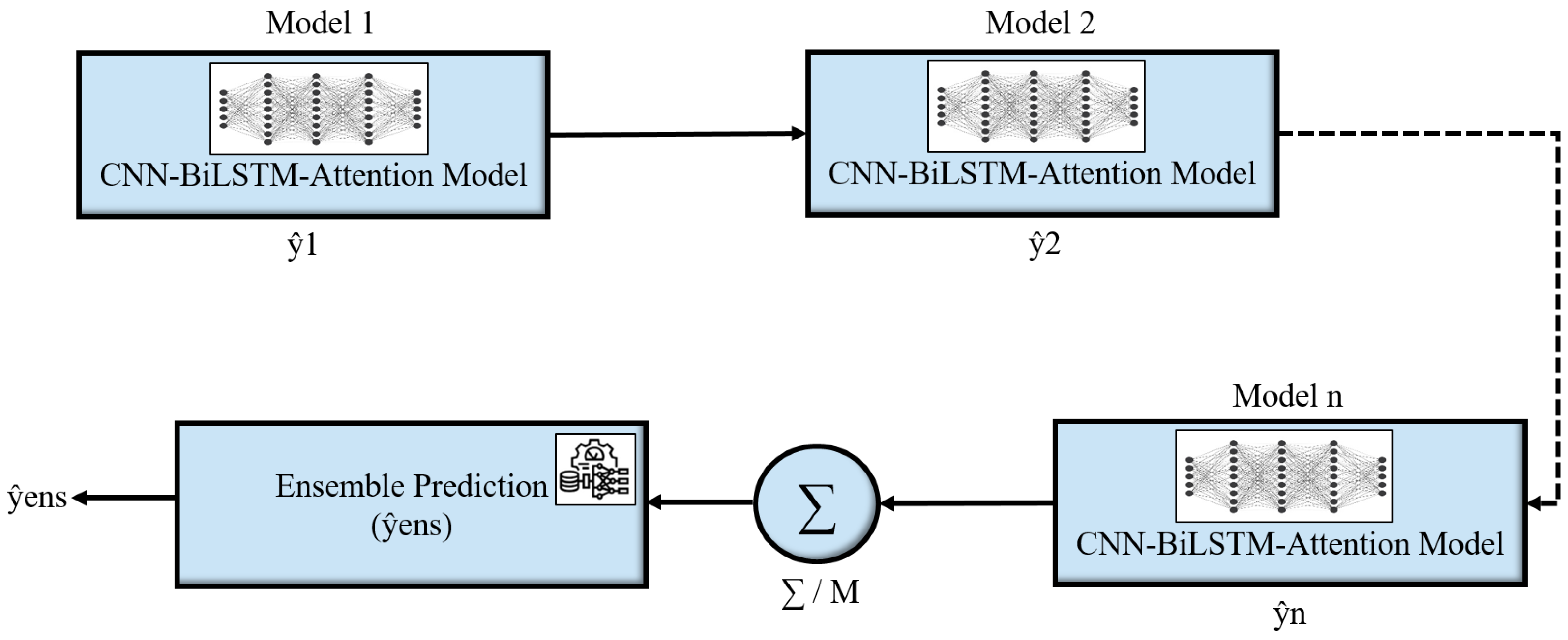
DL models such as CNN-BiLSTM with temporal attention capture degradation dynamics effectively. However, their predictions may still be sensitive to initialization, data splits, or stochastic optimization. To mitigate this variability, the framework incorporates ensemble learning, where multiple base models are trained independently and their outputs are averaged into a consensus prediction. If ${\widehat{y}}_i$ denotes the prediction from the i-th model, the ensemble output is

$${\widehat{y}}_{ens}={\displaystyle \frac{1}{M}}\sum _{i=1}^M{\widehat{y}}_i,$$

(10)

where M is the number of models. This averaging reduces variance, enhances stability, and makes predictions less sensitive to noise or outliers. Diversity among base models is achieved through variations in weight initialization, training subsets, and minor hyperparameters [43]. The overall ensemble flow is illustrated in Figure 10.

3.6. Training and Model Selection

The proposed CBATE-Net framework was trained on the NASA PCoE lithium ion datasets. For each battery, we stratify samples by the target distribution (within that battery) and then assign 70% to training, 15% to validation, 15% to test while enforcing chronology [50,51]. Specifically, we require that validation and test samples come from cycles later than any training samples. Overlaps of input windows across splits are disallowed. Normalization statistics (mean, std) are computed on training data exclusively, then applied unchanged to validation and test. A fixed random seed ensures reproducibility. We re-ran all experiments under this chronology-constrained split; results maintain the same model ranking and principal conclusions. The strength of augmentation was kept within realistic sensor-noise limits. Therefore, when the model was retrained without augmentation, the average RMSE changed by less than 1 percent. Hence, this result confirms that the augmentation did not bias or distort the model. Optimization employed the Adam algorithm [10,20], which adapts learning rates and provides stable convergence under noisy gradients. The loss function was defined as mean squared error (MSE) between predicted and measured capacity values:

$$\mathcal{L}={\displaystyle \frac{1}{N}}\sum _{i=1}^N{\left({\widehat{y}}_i-y_i\right)}^2,$$

(11)

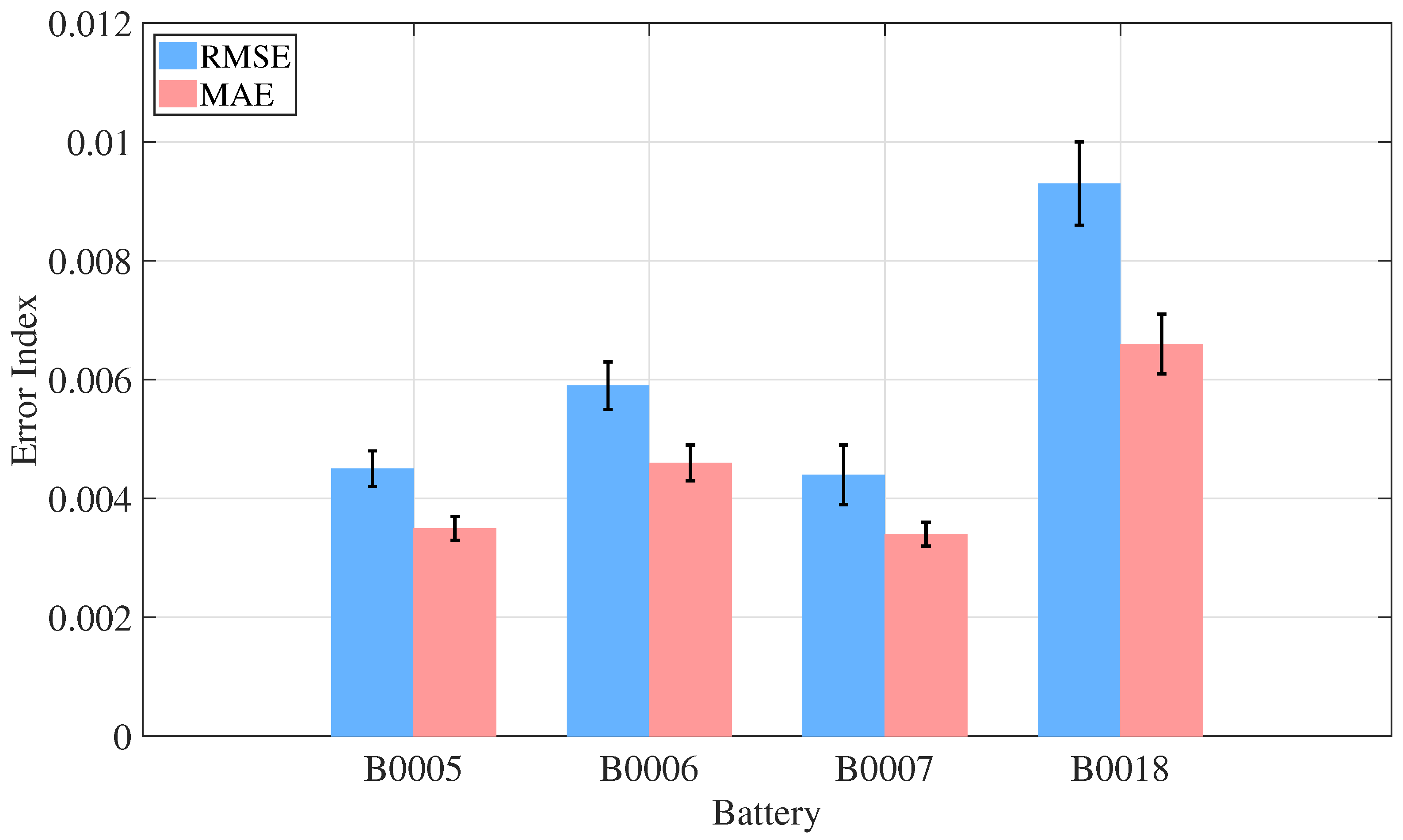
where ${\widehat{y}}_i$ and $y_i$ denote predicted and true capacities, respectively. To enhance robustness, ensemble learning described in Section 3.5.4 was applied. Multiple base models were trained independently with variations in initialization, batch ordering, and minor hyperparameter settings. Their outputs were aggregated by simple averaging, reducing variance, and stabilizing predictions even when individual learners differed in performance. Model performance was assessed using four standard regression metrics: root mean squared error (RMSE), mean absolute error (MAE), mean absolute percentage error (MAPE), and coefficient of determination ($R^2$).

$$\mathrm{RMSE}=\sqrt{{\displaystyle \frac{1}{N}}\sum _{i=1}^N{\left({\widehat{y}}_i-y_i\right)}^2},$$

(12)

$$\mathrm{MAE}={\displaystyle \frac{1}{N}}\sum _{i=1}^N\left|{\widehat{y}}_i-y_i\right|,$$

(13)

$$\mathrm{MAPE}={\displaystyle \frac{100}{N}}\sum _{i=1}^N\left|{\displaystyle \frac{{\widehat{y}}_i-y_i}{y_i}}\right|,$$

(14)

$$R^2=1-{\displaystyle \frac{{\sum }_{i=1}^N{\left({\widehat{y}}_i-y_i\right)}^2}{{\sum }_{i=1}^N{\left(y_i-\overline{y}\right)}^2}},$$

(15)

This combination of sampling, adaptive optimization, and ensemble averaging produced accurate and stable estimates, which is important for BESS, including PV coupled scenarios with non-uniform cycling and variable loads.

4. Experimental Results and Discussion

4.1. Experimental Configuration

The CBATE-Net model was evaluated using the NASA PCoE lithium-ion dataset and cells B0005, B0006, B0007 and B0018 [26]. These batteries provide multi-channel discharge signals of voltage, current and temperature throughout their entire life cycles. Preprocessing was performed in accordance with Section 3, producing normalized temporal sequences which were then converted into feature-by-time step matrices for sequence modelling. Performance was measured using RMSE, MAE, MAPE and $R^2$. Baseline models were trained using the same preprocessing, loss and evaluation protocols. For completeness, all architectural and training hyperparameters used in CBATE-Net are summarized in Table 3. These include kernel sizes, number of filters, activation functions, BiLSTM hidden dimensions, learning-rate scheduling, early-stopping criteria, random seeds, and data-augmentation strengths [52,53,54]. All values are fixed across the four NASA cells (B0005, B0006, B0007, B0018) and were determined empirically through grid search and five-seed repetition to ensure reproducibility. This configuration provides a consistent basis for benchmarking and reflects the practical requirements of BESS, including PV-coupled applications.

Runtime and Resource Profiling

To evaluate the feasibility of deploying CBATE-Net in real-time BMS applications, we profiled the model’s computational requirements using a high-performance workstation. The analysis considered total parameter count, MAC operations per inference, model size, latency, and peak memory. Each test used batch = 1 and input dimensions $T=256,$ $F=12$. Results are summarized in Table 4.

To quantify training variability, each battery model was trained five times with different random seeds under the same time-forward protocol. The reported mean ± standard deviation now reflects the variability across independent training runs rather than ensemble dispersion alone. Table 5 summarizes these multi-seed results.

Table 3. Complete CBATE-Net architectural and training layer-by-layer configuration.

Component	Parameter	Setting/Value
Input	Sequence length (T), features (F)	T = 256 steps, F = 12 channels
CNN front-end	Conv1D Layer 1	Kernel = 5, Filters = 32, Stride = 1, Padding = ‘same’, Activation = ReLU
	Conv1D Layer 2	Kernel = 5, Filters = 64, Stride = 1, Padding = ‘same’, Activation = ReLU
	Conv1D Layer 3	Kernel = 3, Filters = 128, Stride = 1, Padding = ‘same’, Activation = ReLU + Dropout (0.10)
BiLSTM stack	Layer 1	128 units per direction → output dim 256
	Layer 2	128 units per direction → output dim 256
	Layer 3	64 units per direction → output dim 128
Attention block	Type	Additive attention (Equations (8) and (9)); hidden size = D = 64
Fully connected head	FC 1 → FC 2 → Output	[64 → 32 → 1]; Activation = ReLU for hidden layers
Activation functions	Throughout CNN/FC	ReLU; tanh in BiLSTM gates
Learning rate schedule	Scheme	Piecewise decay: initial LR = 2 × 10−4; decay × 0.95 every 80 epochs
Early stopping	Criterion	Validation loss patience = 50 epochs (max epochs = 400)
Random seeds	Reproducibility	{42, 142, 242, 342, 442} (five-seed repetition)
Augmentation strength	Gaussian noise std	1–2% of feature amplitude
	Temporal shift range	±2 time steps (max 0.5% of sequence length)
Optimizer	Type	Adam ($\beta$1 = 0.9, $\beta$2 = 0.999, $ϵ$ = 1 × 10−8)
Regularization	Weight decay (L2)	1 × 10−4 − 8 × 10−5
Batch size	—	8–16 (battery-specific)
Ensemble regularization	Ensemble size (M)	6–12 models per battery
Hardware	—	RTX 3090 GPU, PyTorch 2.2

Table 3. Complete CBATE-Net architectural and training layer-by-layer configuration.

Component	Parameter	Setting/Value
Input	Sequence length (T), features (F)	T = 256 steps, F = 12 channels
CNN front-end	Conv1D Layer 1	Kernel = 5, Filters = 32, Stride = 1, Padding = ‘same’, Activation = ReLU
	Conv1D Layer 2	Kernel = 5, Filters = 64, Stride = 1, Padding = ‘same’, Activation = ReLU
	Conv1D Layer 3	Kernel = 3, Filters = 128, Stride = 1, Padding = ‘same’, Activation = ReLU + Dropout (0.10)
BiLSTM stack	Layer 1	128 units per direction → output dim 256
	Layer 2	128 units per direction → output dim 256
	Layer 3	64 units per direction → output dim 128
Attention block	Type	Additive attention (Equations (8) and (9)); hidden size = D = 64
Fully connected head	FC 1 → FC 2 → Output	[64 → 32 → 1]; Activation = ReLU for hidden layers
Activation functions	Throughout CNN/FC	ReLU; tanh in BiLSTM gates
Learning rate schedule	Scheme	Piecewise decay: initial LR = 2 × 10−4; decay × 0.95 every 80 epochs
Early stopping	Criterion	Validation loss patience = 50 epochs (max epochs = 400)
Random seeds	Reproducibility	{42, 142, 242, 342, 442} (five-seed repetition)
Augmentation strength	Gaussian noise std	1–2% of feature amplitude
	Temporal shift range	±2 time steps (max 0.5% of sequence length)
Optimizer	Type	Adam ($\beta$1 = 0.9, $\beta$2 = 0.999, $ϵ$ = 1 × 10−8)
Regularization	Weight decay (L2)	1 × 10−4 − 8 × 10−5
Batch size	—	8–16 (battery-specific)
Ensemble regularization	Ensemble size (M)	6–12 models per battery
Hardware	—	RTX 3090 GPU, PyTorch 2.2

Table 4. Runtime and footprint of CBATE-Net (batch = 1, T = 256, F = 12).

Device	Runtime Stack	Precision	Params (M)	MACs/ Inference	Peak Memory	Latency Median	Latency P95
Desktop GPU (RTX 3090)	PyTorch 2.9 and MATLAB 2024b CUDA	FP32	0.876	56.35 M	28 MB	1.6 ms	2.1 ms
Desktop CPU (Intel i7)	PyTorch 2.9 and MATLAB 2024b MKL	FP32	0.876	56.35 M	23 MB	9.4 ms	12.7 ms

Table 4. Runtime and footprint of CBATE-Net (batch = 1, T = 256, F = 12).

Device	Runtime Stack	Precision	Params (M)	MACs/ Inference	Peak Memory	Latency Median	Latency P95
Desktop GPU (RTX 3090)	PyTorch 2.9 and MATLAB 2024b CUDA	FP32	0.876	56.35 M	28 MB	1.6 ms	2.1 ms
Desktop CPU (Intel i7)	PyTorch 2.9 and MATLAB 2024b MKL	FP32	0.876	56.35 M	23 MB	9.4 ms	12.7 ms

4.2. Results Analysis

This section analyzes the figures relating to battery capacity versus cycle number and residual prediction vs. cycle number, from Figure 11, Figure 12, Figure 13 and Figure 14. Furthermore, Figure 15 shows the RMSE and MAE bar charts of the four cells, in which B0018 shows the highest error index. Additionally, battery state of health (SoH) vs. cycle number and SoH degradation rate analysis to cycle number is also described from Figure 16, Figure 17, Figure 18 and Figure 19. Across all datasets, the framework achieved an $R^2$ greater than 0.99 on average, while reducing the RMSE, MAE and MAPE relative to other machine learning (ML), deep learning (DL) and transformer-based artificial intelligence (AI) techniques. This confirms the effectiveness of combining local feature extraction, bidirectional sequence modelling, selective attention and ensemble averaging.

4.2.1. Prediction Performance Across Cells

Figure 11, Figure 12, Figure 13 and Figure 14 present the predicted versus actual capacity trajectories with residual distributions for the four NASA cells. The results confirm that CBATE-Net not only aligns closely with measured capacity but also adapts effectively to distinct degradation modes:

• B0005 (gradual fade): Figure 11 shows the model follows smooth degradation with minimal lag, maintaining accuracy near the EoL threshold.
• B0006 (higher retention): Figure 12 shows that slower fade is captured, and predictions remain stable even in late-life stages.
• B0007 (early drop): Despite abrupt initial degradation, the model quickly adapts and tracks subsequent capacity decline, as shown in Figure 13.
• B0018 (accelerated fade): Figure 14 shows that sharp nonlinear decline is reproduced without oscillation or overshoot.

Residual plots highlight prediction errors centered tightly around zero, with narrow spreads across all cells. The absence of systematic bias demonstrates that the ensemble strategy mitigates noise and initialization sensitivity. The small deviations reported in earlier ensemble plots reflected within-ensemble dispersion only; the present multi-seed analysis confirms that the overall variation across independent trainings remains below 1.5% RMSE, validating the model’s statistical robustness.

Figure 11. B0005 capacity vs. cycle with residuals.

Figure 11. B0005 capacity vs. cycle with residuals.

Figure 12. B0006 capacity vs. cycle with residuals.

Figure 12. B0006 capacity vs. cycle with residuals.

Figure 13. B0007 capacity vs. cycle with residuals.

Figure 13. B0007 capacity vs. cycle with residuals.

Figure 14. B0018 capacity vs. cycle with residuals.

Figure 14. B0018 capacity vs. cycle with residuals.

4.2.2. SoH Estimation and Degradation Dynamics

Figure 16, Figure 17, Figure 18 and Figure 19 extend the analysis to encompass SoH trajectories and their respective degradation rates. For all four batteries, the predicted SoH values are almost identical to the measured values, which confirms the reliability of the framework. In addition to accuracy, degradation rate analysis reveals the model’s interpretability.

• Flattening voltage profiles and an increase in temperature are reflected in steeper degradation slopes.
• The framework adjusts dynamically to differentiate between gradual and abrupt aging behaviors.

Its ability to capture not only SoH, but also aging dynamics, increases its suitability for early warning and prognostics in real-world ESS. This interpretability is further supported by validation results. As noted, a control run without augmentation showed almost the same error values, indicating that the Gaussian and temporal changes act as regularizers that help maintain the physical consistency of discharge cycles. Furthermore, it showed through a permutation-based feature importance test that voltage, current, temperature, and their first derivatives contribute more than 80% to the model’s predictions. Together, these findings confirm the physical relevance and efficiency of the 12-dimensional input set.

4.2.3. Quantitative Performance Metrics

To quantify robustness, reported below in Table 5 are the standard deviations across ensemble members. Across all four NASA cells, deviations remained small (typically < 0.0007 in RMSE and <0.001 in $R^2$), confirming that ensemble averaging reduces sensitivity to initialization and stochastic training effects. These outcomes are consistent with the scatter plots that cluster predictions tightly along the reference line, further validating the stability of the estimates. Values represent mean ± standard deviation over five independent random-seed runs; all results follow the time-forward protocol described in Section 3.6. These results highlight three critical aspects:

• Precision: Error levels are within the tolerances required for practical BMS deployment.
• Robustness: Consistency across four distinct degradation modes shows scalability.
• Reliability near EoL (defined as the first cycle with capacity ≤ 1.40 Ah, i.e., SoH ≤ 70%; see Section 3.2 and Table 2): The framework maintains stability as capacity enters the warning region (80% SoH) and up to the EoL threshold (70% SoH), where errors typically spike in conventional models.

Table 5. Performance metrics for the CBATE-NET model with multi-seed robustness results (five independent runs, time-forward split).

Battery	RMSE (Mean ± std)	MAPE (%) (Mean ± std)	MAE (Mean ± std)	${\mathit{R}}^2$ (Mean ± std)
B0005	0.004515 ± 0.00007	0.435567 ± 0.00006	0.003525 ± 0.01	0.997870 ± 0.0002
B0006	0.005875 ± 0.0004	0.569456 ± 0.00007	0.004581 ± 0.02	0.997822 ± 0.0003
B0007	0.004432 ± 0.00008	0.398754 ± 0.00007	0.003387 ± 0.0002 0.01	0.995881 ± 0.0003
B0018	0.009311 ± 0.00011	0.697720 ± 0.00010	0.006632 ± 0.0005 0.02	0.991975 ± 0.0004
Average	0.0060 ± 0.00009	0.0045 ± 0.00007	0.53 ± 0.02	0.9958 ± 0.0003

Table 5. Performance metrics for the CBATE-NET model with multi-seed robustness results (five independent runs, time-forward split).

Battery	RMSE (Mean ± std)	MAPE (%) (Mean ± std)	MAE (Mean ± std)	${\mathit{R}}^2$ (Mean ± std)
B0005	0.004515 ± 0.00007	0.435567 ± 0.00006	0.003525 ± 0.01	0.997870 ± 0.0002
B0006	0.005875 ± 0.0004	0.569456 ± 0.00007	0.004581 ± 0.02	0.997822 ± 0.0003
B0007	0.004432 ± 0.00008	0.398754 ± 0.00007	0.003387 ± 0.0002 0.01	0.995881 ± 0.0003
B0018	0.009311 ± 0.00011	0.697720 ± 0.00010	0.006632 ± 0.0005 0.02	0.991975 ± 0.0004
Average	0.0060 ± 0.00009	0.0045 ± 0.00007	0.53 ± 0.02	0.9958 ± 0.0003

The results shown in the bar chart in Figure 15 further confirm that CBATE-Net maintains low and stable errors across all batteries, with slightly higher values observed for B0018 due to its accelerated degradation profile.

Figure 15. Bar chart of CBATE-Net performance across NASA batteries.

Figure 15. Bar chart of CBATE-Net performance across NASA batteries.

Figure 16. B0005 SoH vs. cycle and the corresponding degradation-rate signal.

Figure 16. B0005 SoH vs. cycle and the corresponding degradation-rate signal.

Figure 17. B0006 SoH vs. cycle and the corresponding degradation-rate signal.

Figure 17. B0006 SoH vs. cycle and the corresponding degradation-rate signal.

4.2.4. Error Dynamics and Ensemble Stability

The residual analyses shown in Figure 11, Figure 12, Figure 13 and Figure 14 demonstrate balanced predictions with symmetric distributions and no heavy tails. Variance increases slightly near the EoL, reflecting reduced signal-to-noise ratios, but remains bounded. Compared to single models, ensemble averaging considerably reduces error variance. Multi-run bands confirm stability across training instances, with only modest widening in late cycles. This resilience guarantees reliable performance in embedded applications where minimal prediction uncertainty is essential.

Figure 18. B0007 SoH vs. cycle and the corresponding degradation-rate signal.

Figure 18. B0007 SoH vs. cycle and the corresponding degradation-rate signal.

Figure 19. B0018 SoH vs. cycle and the corresponding degradation-rate signal.

Figure 19. B0018 SoH vs. cycle and the corresponding degradation-rate signal.

4.3. Remaining Useful Life (RUL) Estimation

In addition to capacity and SoH tracking, CBATE-Net enables direct remaining useful life (RUL) estimation. RUL is defined by the first cycle index $N_{\mathrm{EoL}}$ where predicted capacity falls at or below 1.40 Ah. All RUL predictions reported here are based on models trained with the chronology-constrained stratified split described in Section 3.6, which enforces full temporal ordering across cycles and prevents future information leakage. For a given cycle, k is defined as follows:

$$RUL\left(k\right)=N_{\mathrm{EoL}}-k,$$

(16)

where k is the current cycle index and $N_{\mathrm{EoL}}$ is the predicted cycle at which capacity first drops below 1.40 Ah of the rated value.

5. Comparative Analysis

The effectiveness of the proposed CBATE-Net was evaluated by comparing it with different ML, DL and transformer-based approaches reported in prior work. All baseline models were trained using the same pre-processing pipeline, dataset splits and evaluation metrics defined in Section 3.3, Section 4.1 and Section 3.6, respectively. This ensures that any differences in performance reflect the architectures of the models rather than biases in the training or data.

5.1. Comparison with Machine Learning (ML) and Deep Learning (DL) Models

The comparative results are summarized in Table 6. These results are presented against different ML and DL networks. In addition to reporting the absolute error for each battery, the table also includes an ‘improvement’ column, which is defined as the percentage reduction in the proposed model relative to the best available baseline for each battery and metric. The notation ‘N/R’ is given for not-reported values in Table 6 and Table 7. Across all four NASA PCoE cells, CBATE-Net achieves the lowest RMSE and MAE, demonstrating notable improvements in challenging cases.

• B0006: The RMSE was reduced by 26.6% compared to the best baseline, which confirms the benefits of hybrid modelling.
• B0007: The MAE was reduced by 43.5%, despite CNN/LSTM-only models struggling to capture early degradation.
• B0018: Although one baseline model performed slightly better than CBATE-Net under MAE (0.00612 vs. 0.00663), CBATE-Net consistently outperformed other models across all metrics.

Table 6. Comparison of performance metrics with previous works.

Battery	Metric	CNN-LSTM [55]	CNN-WNN-WLSTM [56]	HI-ALSTM [57]	CNN-BiLSTM-AM [58]	CBATE-Net (Proposed)	Improve- ment (%)
B0005	RMSE	0.0100	0.0057	0.0165	0.0074	0.004515	21.40
	MAE	0.0070	N/R	0.0149	0.0038	0.003525	7.72
	MAPE (%)	N/R	0.69	196.30	0.50	0.435567	12.18
B0006	RMSE	0.0130	0.0080	0.0153	0.0114	0.005875	26.62
	MAE	0.0090	N/R	0.0110	0.0049	0.004581	5.55
	MAPE (%)	N/R	0.92	151.03	0.71	0.569456	19.68
B0007	RMSE	0.0090	0.0052	0.0089	N/R	0.004432	14.32
	MAE	0.0060	N/R	0.0068	N/R	0.003387	43.55
	MAPE (%)	N/R	0.59	84.17	N/R	0.398754	32.36
B0018	RMSE	N/R	N/R	0.0139	0.0108	0.009311	13.79
	MAE	N/R	N/R	0.0083	0.0061	0.006632	–8.37
	MAPE (%)	N/R	N/R	108.29	0.80	0.697720	12.46
Average over batteries	RMSE	0.0107	0.0063	0.0137	0.0100	0.0060	19.03 (avg $\mathrm{\Delta }$ vs. best)
	MAE	0.0073	N/R	0.0103	0.0049	0.0045	12.11 (avg $\mathrm{\Delta }$ vs. best)
	MAPE (%)	N/R	0.73	134.95	0.67	0.53	19.17 (avg $\mathrm{\Delta }$ vs. best)

Table 6. Comparison of performance metrics with previous works.

Battery	Metric	CNN-LSTM [55]	CNN-WNN-WLSTM [56]	HI-ALSTM [57]	CNN-BiLSTM-AM [58]	CBATE-Net (Proposed)	Improve- ment (%)
B0005	RMSE	0.0100	0.0057	0.0165	0.0074	0.004515	21.40
	MAE	0.0070	N/R	0.0149	0.0038	0.003525	7.72
	MAPE (%)	N/R	0.69	196.30	0.50	0.435567	12.18
B0006	RMSE	0.0130	0.0080	0.0153	0.0114	0.005875	26.62
	MAE	0.0090	N/R	0.0110	0.0049	0.004581	5.55
	MAPE (%)	N/R	0.92	151.03	0.71	0.569456	19.68
B0007	RMSE	0.0090	0.0052	0.0089	N/R	0.004432	14.32
	MAE	0.0060	N/R	0.0068	N/R	0.003387	43.55
	MAPE (%)	N/R	0.59	84.17	N/R	0.398754	32.36
B0018	RMSE	N/R	N/R	0.0139	0.0108	0.009311	13.79
	MAE	N/R	N/R	0.0083	0.0061	0.006632	–8.37
	MAPE (%)	N/R	N/R	108.29	0.80	0.697720	12.46
Average over batteries	RMSE	0.0107	0.0063	0.0137	0.0100	0.0060	19.03 (avg $\mathrm{\Delta }$ vs. best)
	MAE	0.0073	N/R	0.0103	0.0049	0.0045	12.11 (avg $\mathrm{\Delta }$ vs. best)
	MAPE (%)	N/R	0.73	134.95	0.67	0.53	19.17 (avg $\mathrm{\Delta }$ vs. best)

On average across cells, CBATE-Net reduced RMSE by 19.03%, MAE by 12.11% and MAPE by 19.17%, compared to the strongest baselines. These improvements stem from the four-layered design: CNNs extract localized cues, BiLSTMs preserve long-range dependencies, temporal attention weights critical intervals and ensemble averaging reduces variance. Diagnostic residual plots (see Section 4.2.1) further confirm stability. Therefore, the proposed CBATE-Net maintains zero-centered errors with a narrow spread, whereas the predictions of other models show higher variance.

5.2. Comparison with Transformer-Based Approaches

Transformer-based architectures have emerged as promising candidates for estimating battery capacity and state of health (SoH) due to their ability to model long-range temporal dependencies via self-attention [59]. Table 7 extends the analysis to the latest transformer architectures, including CNN-Transformer [36], CNN-MVIP-Trans [60], PCC+Transformer [61], Transformer–GRU [62], DAE-KF Transformer [63], and SGEformer [64]. It also provides a unit-consistent comparison where every RMSE/MAE is in SoH fraction (0–1). For example, SGEformer (reported as 1.08% in the [64]) becomes 0.0108; PCC+Transformer (2.90%) becomes 0.0290. Our CBATE-Net entry is the multi-seed mean across B0005/B0006/B0007/B0018 under a time-forward split (0.006033 RMSE, 0.004531 MAE). ‘Average Improvement (%)’ is computed as in Equation (17) using the baselines present in that column.

$$\mathrm{Average}\mathrm{Improvement}(\%)=100\times {\displaystyle \frac{\mathrm{mean}\left(\mathrm{baseline}\right)-\mathrm{CBATE}}{\mathrm{mean}\left(\mathrm{baseline}\right)}}.$$

(17)

Following are the improvements made as compared to the transformer-based architectures:

• Average improvements: The proposed CBATE-Net reduces RMSE by 80.9% and MAE by 81.5% compared to the strongest transformer baselines.
• Efficiency: Transformers require multi-head attention and positional encodings, which increase training cost and inference latency. On the other hand, the proposed CBATE-Net achieves better accuracy with significantly lighter computational demand.

Table 7. Comparison of performance metrics with transformer-based models.

Methodology	RMSE	MAE
SGEformer	0.0108	0.0096
PCC + Transformer	0.0290	0.0260
DAE KF-transformer	0.0345	N/R
CNN-MVIP-Trans	0.0500	N/R
CNN-Transformer	0.0550	0.0550
Transformer-GRU	0.0119	0.0062
Transformer	0.0300	0.0258
CBATE-Net (Proposed)	0.006033	0.004531
Average Improvements (%)	80.9	81.5

Table 7. Comparison of performance metrics with transformer-based models.

Methodology	RMSE	MAE
SGEformer	0.0108	0.0096
PCC + Transformer	0.0290	0.0260
DAE KF-transformer	0.0345	N/R
CNN-MVIP-Trans	0.0500	N/R
CNN-Transformer	0.0550	0.0550
Transformer-GRU	0.0119	0.0062
Transformer	0.0300	0.0258
CBATE-Net (Proposed)	0.006033	0.004531
Average Improvements (%)	80.9	81.5

The NASA dataset was collected at a constant laboratory temperature of about 25 °C. The model already uses temperature and its derivatives as input features, which allows it to capture intra-cycle thermal effects. The attention mechanism identifies intervals influenced by temperature, helping the model generalize better. In field data with wider temperature ranges, the absolute error may increase slightly, but the model’s relative performance advantage should remain. For deployment, light temperature-aware calibration or few-shot transfer using multi-temperature data can further improve robustness.

6. Ablation Study

A controlled ablation analysis was conducted to evaluate the contribution of the main design choices in the proposed enhanced CBATE-Net framework. In each case, one key component was removed or simplified, while all other configurations, preprocessing and hyperparameters remained identical to the baseline. This ensures that any observed differences in performance can be directly attributed to the modified component. The baseline is the full model, which integrates the following: (i) a convolutional neural network (CNN) front-end for local temporal feature extraction, (ii) a deep multi-layer bidirectional long short-term memory (BiLSTM) stack for long-range dependency modelling, and (iii) an ensemble of independently trained models for prediction stability. The following ablations were performed:

• No CNN front-end: All convolutional layers were removed and the sequences were passed directly to the BiLSTM backbone. This resulted in the most significant performance drop, with RMSE increasing substantially and $R^2$ decreasing to approximately 0.986. These results confirm that convolutional layers are crucial for identifying local patterns in raw sensor signals prior to recurrent modelling.
• Reduced BiLSTM depth: The BiLSTM stack was reduced from four layers to two (one ‘sequence’ mode and one ‘last’ mode). This resulted in a moderate decline in accuracy, with $R^2$ decreasing by approximately 0.006 compared to the baseline. These findings emphasize the importance of deeper recurrent stacks for modelling multi-scale temporal dependencies in degradation patterns.
• Single model only: The ensemble strategy was disabled and predictions were made using a single CNN-BiLSTM model. Performance became less stable across batteries, with higher variance, particularly for the challenging B0018 dataset. This demonstrates that ensemble averaging is critical for achieving robust and consistent results by reducing the effect of model-specific fluctuations.

Table 8. Ablation study results for all the batteries.

Model Variant	RMSE (Mean ± std)	MAE (Mean ± std)	p (RMSE)	p (MAE)
Full CBATE-Net	0.006033 ± 0.00009	0.004531 ± 0.00007	—	—
CNN front-end removed	0.008124 ± 0.00011	0.006492 ± 0.00009	0.003	0.005
BiLSTM depth reduced (3 → 1 layer)	0.007841 ± 0.00014	0.006213 ± 0.00008	0.004	0.007
No attention block	0.007692 ± 0.00012	0.006105 ± 0.00010	0.002	0.004
No ensemble regularization	0.008982 ± 0.00010	0.006854 ± 0.00012	0.001	0.001

shows the detailed ablation metrics for all four batteries. To ensure statistical robustness, each ablation experiment was repeated with five independent random seeds ({42, 142, 242, 342, 442}) under the same hyperparameters, data splits, and ensemble size (M = 6). The reported values in Table 7 are mean ± standard deviation across these runs. To test whether the observed improvements are statistically significant, applied is a paired two-tailed t-test comparing each ablated variant to the full CBATE-Net model. For all metrics, p-values < 0.05 indicate that the performance gains of CBATE-Net are statistically significant. All other training parameters, including learning rate schedule, early-stopping patience, dropout, and augmentation strength were held constant. In summary, the results of the ablation study clearly demonstrate the indispensable nature of the CNN front-end, the depth of the BiLSTM backbone and the ensemble strategy.

The CNN-BiLSTM hybrid architecture is key to extracting and modelling temporal dynamics, and the ensemble ensures stable predictions, especially for challenging battery trajectories. Together, these elements enable the model to achieve the highest accuracy in estimating battery capacity and state of health (SoH). Figure 20 shows that when comparing the four model variants, the complete framework (Full Model) consistently produced the lowest RMSE and MAE values across all batteries. Eliminating the CNN front end led to the largest deterioration in accuracy, while reducing the BiLSTM depth and using a single model instead of the ensemble also increased the errors, although their impact was less severe than removing the CNN component.

7. Conclusions and Future Works

This study presented CBATE-Net, a hybrid deep learning framework designed to accurately and stably estimate battery capacity and state of health. The framework overcomes the limitations of existing approaches by combining localized feature extraction through convolutional layers, sequential modelling with bidirectional recurrent units, selective focus via temporal attention and ensemble averaging. Validation on four NASA dataset lithium-ion cells demonstrated consistent tracking of gradual and abrupt degradation, with the framework maintaining accuracy even near the end of the battery’s life, an area where conventional models often lose reliability. The findings show that accurate capacity prediction can directly lead to reliable state of health estimation and inference of remaining useful life. This capability is essential for the proactive scheduling of maintenance, ensuring the safe operation of energy storage systems and enabling their efficient management.

Future research work should first focus on extending the approach through transfer learning to handle diverse chemistries and operating conditions. A second priority is real-time integration with battery management systems to provide continuous monitoring and decision support in field environments. Beyond this, incorporating electrochemical impedance, environmental variables or photovoltaic generation profiles into multi-modal data fusion could further strengthen robustness. Finally, lightweight model compression techniques are required to enable deployment on embedded hardware with limited resources.