Investigating the Asymmetric Impact of Renewable and Non-Renewable Energy Production on the Reshaping of Future Energy Policy and Economic Growth in Greece Using the Extended Cobb–Douglas Production Function

Abstract

This paper investigates the symmetric and asymmetric effects of renewable and non-renewable energy on Greece’s economic growth within an extended Cobb–Douglas production function for 1990–2022. The study is motivated by the rising role of renewable energy and the need to determine whether the energy–growth nexus is linear or nonlinear, an issue of central importance for policy. The Brock–Dechert–Scheinkman (BDS) test confirms the nonlinearity of the variables, while Zivot–Andrews unit root tests with structural breaks capture crisis-related disruptions. The Wald test indicates that renewable energy has an asymmetric long-run relationship with growth, whereas non-renewables exert symmetric effects. To model these dynamics, the Nonlinear Autoregressive Distributed Lag (NARDL) framework is applied. Results show that in the long run, positive shocks to renewable energy enhance growth, while both positive and negative shocks to non-renewables have symmetric impacts. In the short run, only non-renewable energy shocks significantly affect growth. Asymmetric causality analysis reveals a bidirectional relationship between positive renewable shocks and growth, suggesting a virtuous cycle of renewable expansion and economic performance. The study contributes by providing the first systematic evidence for Greece on the nonlinear energy–growth nexus, advancing empirical modeling with NARDL and break-adjusted tests, and highlighting the heterogeneous growth effects of renewable versus non-renewable energy.

1. Introduction

Energy is considered one of the fundamental tools for improving living conditions, economic production, and, therefore, development. Over the last few years, the demand for energy has increased significantly due to population growth, transport, services, and especially the spread of industrialization. The increased demand is largely met by non-renewable energy sources, resulting in increased negative externalities in the energy system, contributing to climate change as well as other environmental problems. Renewable energy sources, as supported by Persis [1], apart from being a growth lever and a solution to the depletion of natural resources, also help reduce pollution from CO₂ emissions. The success of renewable energy sources is due to their contribution to environmental sustainability and, therefore, to the fight against climate change, which has found general political and public acceptance. An additional benefit of renewable energy sources is their contribution to energy supply, i.e., energy security.

High-income economies, such as the EU countries, have been responding to the Paris Agreement since 2015 by promoting green technology and implementing legal agreements to mitigate climate change. Implementing this framework for the transition to alternative energy sources from renewable sources across all EU countries requires social and economic reforms. The production of renewable energy sources creates new jobs, contributes to increasing income either through increasing productivity or through the creation of new jobs, and stimulates economic development in regions and at the local level. The rise in energy prices observed in the Russia–Ukraine war has resulted mainly in low- and middle-income EU countries securing an energy supply. The provision of energy supply comes from both renewable and non-renewable sources.

Greece already has quite significant potential from renewable energy sources, which can offer a real alternative solution for meeting its energy needs. However, it can certainly make even more use of sun and wind by increasing the percentage of its energy needs covered by renewable energy sources, limiting its carbon footprint and exceeding European directives. The implementation of relevant initiatives will minimize the need for energy imports, while safeguarding its energy security. Greece occupies one of the highest positions in the penetration rate of renewable energy sources in its energy mix, according to the Ember report in 2022. With 20.7% of electricity coming from wind turbines and 12.6% from photovoltaics, the total contribution of renewable energy sources to Greece’s energy mix reached 33.3%. A percentage that brings Greece in seventh place worldwide in terms of the penetration of renewable energy sources in electricity production [2].

The introduction of natural gas into Greece’s energy balance is expected to affect important sectors of the country’s economic and social life, and ensure the diversification of energy sources in the country, with a high-quality fuel that can penetrate almost all sectors (industry, electricity generation, cogeneration, services and the residential sector, transport, etc.). With the introduction of natural gas, the following are expected:

• The increase in the competitiveness of Greek industry.
• A reduction in air pollution.
• Improvement in the quality of life.
• The creation of new jobs.

The inclusion of renewable and non-renewable energy sources as inputs in the production process is grounded in the extended endogenous growth theory and the augmented Cobb–Douglas production framework. In these models, energy is not merely an intermediate input but a critical driver of productivity and long-run growth [3,4]. Energy consumption enhances the efficiency of capital and labor, while constraints or volatility in energy supply can limit output.

Within the energy–growth nexus literature, two main hypotheses prevail:

• The growth hypothesis (energy use drives output growth);
• The conservation hypothesis (growth drives energy demand), with empirical evidence often showing bidirectional causality depending on the type of energy considered [5,6].

The case of Greece provides a compelling context: abundant but underutilized renewable resources (solar, wind, and biomass), heavy dependence on imported fossil fuels, and the inability to safely exploit nuclear power due to high seismicity. EU subsidies and energy transition policies further increase the relevance of assessing how different forms of energy contribute to growth.

The role of asymmetry is theoretically justified by adjustment-cost models and behavioral responses: positive shocks to renewables (e.g., investment or policy support) may stimulate output differently than negative shocks (e.g., policy withdrawal), while fossil fuels often exert symmetric effects due to their entrenched role in production systems [7,8].

Based on this background, the study raises the following hypotheses:

H1. 

Inflows of renewable and non-renewable energy sources affect economic growth in Greece through both long-term equilibrium and short-term dynamics.

H2. 

Positive and negative shocks to renewable and non-renewable energy exert asymmetric effects on economic growth in the long and short run.

H3. 

There exists an asymmetric causal relationship between renewable and non-renewable energy sources and economic growth, the direction of which may differ by energy type.

This paper makes several contributions to the literature:

• Extension of the production function: By incorporating renewable and non-renewable energy into the Cobb–Douglas framework, the paper expands traditional growth models to explicitly account for energy as a production factor in Greece.
• Asymmetric modeling approach: The use of the Nonlinear Autoregressive Distributed Lag (NARDL) model allows us to disentangle the effects of positive versus negative shocks in energy consumption on growth, a methodological novelty for the Greek context.
• Context-specific insights: The study provides the first evidence for Greece that compares the asymmetric contributions of renewable versus non-renewable energy to growth over a long period marked by structural shocks (financial crises and EU energy transition policies).
• Causality dynamics: By examining asymmetric causality, the paper reveals whether growth and energy dynamics reinforce one another differently depending on energy type and shock direction.
• Policy relevance: The findings contribute to policy debates on energy security and sustainable development, showing whether renewable expansion can mitigate Greece’s reliance on volatile fossil fuel imports.

The paper is organized as follows. The next section presents a literature review. Section 3 presents the methodology. Empirical results and discussion are presented in Section 4. Section 5 presents conclusions and recommendations.

2. Literature Review

The empirical literature on the energy–growth nexus yields mixed findings, reflecting heterogeneity in econometric methods, sample periods, and national contexts. Three primary transmission channels have been emphasized: (i) productivity effects, whereby energy enhances output directly as a factor of production; (ii) factor substitution effects, where renewable and non-renewable energy interact with capital and labor inputs; (iii) induced innovation, in which renewable adoption stimulates complementary investment in technology and research. A further unresolved dimension is the presence of asymmetric effects, including the differential impacts of positive and negative shocks, as well as the varying influence of renewable compared to fossil sources across short-run and long-run horizons.

Early evidence supports the productivity channel. Sari [9], examining six developing economies, showed that energy can, in some cases, outweigh labor and capital in explaining output dynamics. Ruhul [10] demonstrated long-run co-integration and bidirectional causality between energy consumption and industrial production in OECD economies, reinforcing the centrality of energy to productivity. In Greece, Dergiades [11] similarly identified strong causal links between useful energy consumption and growth, even under nonlinear specifications, underscoring the energy dependence of a crisis-prone economy.

Studies focusing on induced innovation highlight the complementary role of research and technology. Inglesi [12] reported that renewable energy consumption, when paired with R&D spending, positively and significantly affects economic growth across OECD countries. This resonates with findings for Greece: Dritsaki [2,13] provides evidence that renewable energy fosters long-run growth and interacts with human capital development, suggesting that innovation capacity is critical for sustained benefits from renewable deployment.

Substitution and heterogeneity have been highlighted in comparative studies. Halicioglu [14], analyzing 15 EU countries, found co-integration in fewer than half, with varying relative effects of renewables and non-renewables. Okumuş [15] confirmed that both energy types support growth in the G7, though non-renewables still dominate. For Greece, Triantafyllidou [16] identified strong source-specific causalities, including a long-run effect of wind energy on GDP per capita, yet fossil fuels remain the primary energy driver, reflecting incomplete substitution during the transition.

In low-and middle-income contexts, the evidence is more complex. Afzal [17] introduced the notion of a “renewable energy curse” or “paradox of plenty”, finding that renewable abundance may crowd out human capital development when institutions and complementary investments are weak. Similar path dependencies are observed in Asia, where fossil fuel consumption continues to constrain renewable integration [18]. These results caution against directly extrapolating OECD evidence to crisis-affected or institutionally constrained economies.

Asymmetries remain a critical unresolved issue. While Okumuş [15] suggests stronger non-renewable impacts, and Greek studies document nonlinear and source-specific dynamics [11,16], systematic evidence distinguishing short-run versus long-run asymmetries is scarce. Addressing these dynamics is essential for policy design, particularly in countries vulnerable to shocks and structural breaks.

Finally, the literature increasingly situates the energy–growth nexus within a geopolitical context. Hashemizadeh [19] emphasizes how China’s technological leadership in solar, wind, and batteries, combined with Belt and Road Initiative (BRI) financing, is reshaping global renewable energy diffusion. For smaller, crisis-exposed economies such as Greece, these dynamics imply both opportunities, via lower technology costs and expanded innovation spillovers, and risks, including new forms of dependence and external policy conditionalities. Such geopolitical drivers may alter the balance between productivity, substitution, and innovation channels, while also amplifying or mitigating asymmetric effects.

Overall, the literature suggests that energy contributes robustly to growth; however, the dominant channel (productivity, substitution, or innovation) depends on structural and institutional conditions. Evidence from OECD and G7 countries generally confirms the long-run growth benefits of renewables, whereas studies on Greece and other crisis-affected economies point to nonlinearities, source-specific asymmetries, and potential crowding-out effects in the absence of robust human-capital and innovation policies. What remains unresolved is how asymmetric shocks propagate across contexts and how geopolitically mediated technology and finance flows will shape the next stage of the transition.

3. Methodology

3.1. Model Specification

Cobb’s [20]’s function describes the relationship between the inputs of capital and labor and output in a production process. It assumes constant returns to scale, with parameters interpreted as elasticities of production inputs. To capture the role of energy as a key production factor, the function is extended to include energy, preserving its structural integrity. The function below can also be called the Cobb–Douglas production function of augmented energy.

$$Q=A{K}^{{\beta }_1}{L}^{{\beta }_2}{E}^{{\beta }_3}.$$

(1)

According to the work of [21,22], the production process of Function (1) is based on two types of energy: energy from renewable sources and energy from non-renewable sources. Therefore, Function (1) can be modified to take into account the use of both sources of energy. Therefore, Function (1) is adjusted as follows:

$$Q=A{K}^{{\beta }_1}{L}^{{\beta }_2}R{E}^{{\beta }_3}NR{E}^{{\beta }_4}..$$

(2)

The variables $RE$ and $NRE$ are used to denote renewable and non-renewable energy sources. The parameters ${\beta }_3$ and ${\beta }_4$ describe the response of production to changes in renewable and non-renewable energy, respectively.

Renewable energy sources refer to wind and solar energy, hydroelectric power, geothermal energy, and biomass. Non-renewable energy sources refer to oil, coal, and natural gas.

In the model described above, real gross domestic product $(GDP)$ serves as the dependent variable, while the independent variables include capital $(K)$, labor $(L)$, renewable energy $(RE)$, and non-renewable energy $(NRE)$. The exponents ${\beta }_1$, ${\beta }_2$, ${\beta }_3$, and ${\beta }_4$ are the elasticities of production in relation to capital, labor, renewable, and non-renewable sources, respectively.

By applying natural logarithms to all variables of Function (2), we transform it into a log-linear form to smooth out sharp fluctuations and to make the coefficients interpretable as elasticities. The resulting function takes the following form:

$$\ln GD{P}_t={\beta }_0+{\beta }_1\ln K_t+{\beta }_2\ln L_t+{\beta }_3\ln R{E}_t+{\beta }_4\ln NR{E}_t+e_t.$$

(3)

${\beta }_0$ denotes a constant factor, and ${\beta }_1$, ${\beta }_2$, ${\beta }_3$, and ${\beta }_4$ represent measures of how production changes in terms of capital, labor, renewable and non-renewable energy sources, respectively. $e_t$ is an error term.

The relationship between renewable energy sources and economic growth is expected to be positive according to the work of [23,24], which highlights the significant impact of renewable energy sources on economic growth, showing that the increase in the use of renewable energy sources is accompanied by economic expansion.

Thus, we will have ${\beta }_3={\displaystyle \frac{\ln GD{P}_t}{\ln R{E}_t}}>0$. Also, the relationship between non-renewable energy sources and economic growth is expected to be positive according to the work of [25,26,27]. So, we will have ${\beta }_4={\displaystyle \frac{\ln GD{P}_t}{\ln NR{E}_t}}>0$. The link between capital, labor, and economic growth was studied by [21,22], and they demonstrated that capital and labor are positively associated with economic growth. On the other hand, the studies of [28,29] determine that employment is negatively correlated with economic growth. So, we will have ${\beta }_1={\displaystyle \frac{\ln GD{P}_t}{\ln K_t}}>0$ and ${\beta }_2={\displaystyle \frac{\ln GD{P}_t}{\ln L_t}}>0$ or ${\beta }_2={\displaystyle \frac{\ln GD{P}_t}{\ln L_t}}<0$.

However, in our study, a positive relationship between capital and economic growth, a positive relationship between renewable and non-renewable energy sources, as well as a positive or negative relationship between labor and economic growth, is expected.

3.2. Data

The data sample consists of annual time series for the period 1990 to 2022 and comes from the World Development Indicators. GDP is in millions of USD in constant 2015 prices. GFC is the gross fixed capital formation as a % of GDP. LFP is the total labor force. RE is electricity production from renewable sources such as wind and solar, hydroelectricity, geothermal, and biomass as a % of the total in kWh. NRE is electricity production from non-renewable energy sources such as oil, coal, and natural gas as a % of the total in kWh.

Table 1. Variable descriptions and sources.

Variable	Code	Defnition	Source
Gross domestic product	GDP	GDP at purchaser’s prices is the sum of gross value added by all resident producers in the economy, plus any product taxes and minus any subsidies not included in the value of the products	World Bank Development Indicators Constant 2015 USD
Gross fixed capital formation	GFC	Gross fixed capital formation consists of outlays on additions to the fixed assets of the economy, plus net changes in the level of inventories	World Bank Development Indicators Constant 2015 USD
Total labor force	LFP	The total labor force comprises people ages 15 and older who supply labor for the production of goods and services during a specified period	World Bank Development Indicators Millions
Renewable energy	RE	Renewable energy includes wind, solar, hydroelectricity, geothermal, and biomass	World Energy Statistical Review kWh
Non-renewable energy	NRE	Non-renewable energy includes oil, coal. and natural gas	World Energy Statistical Review kWh

Sources: [30,31].

describes the variables and data sources.

Table 2. Descriptive statistics.

	Mean	Std. Dev.	Skew.	Kurt.	J.Β	Prob.	Obs.
LGDP	26.031	0.149	0.220	2.211	1.122	0.570	33
LGFC	2.880	0.335	−0.460	1.483	4.327	0.114	33
LLFP	15.370	0.057	−0.936	3.067	4.830	0.089	33
LRE	11.275	0.343	0.234	1.734	2.504	0.285	33
LNRE	13.752	0.169	0.199	2.007	1.573	0.455	33

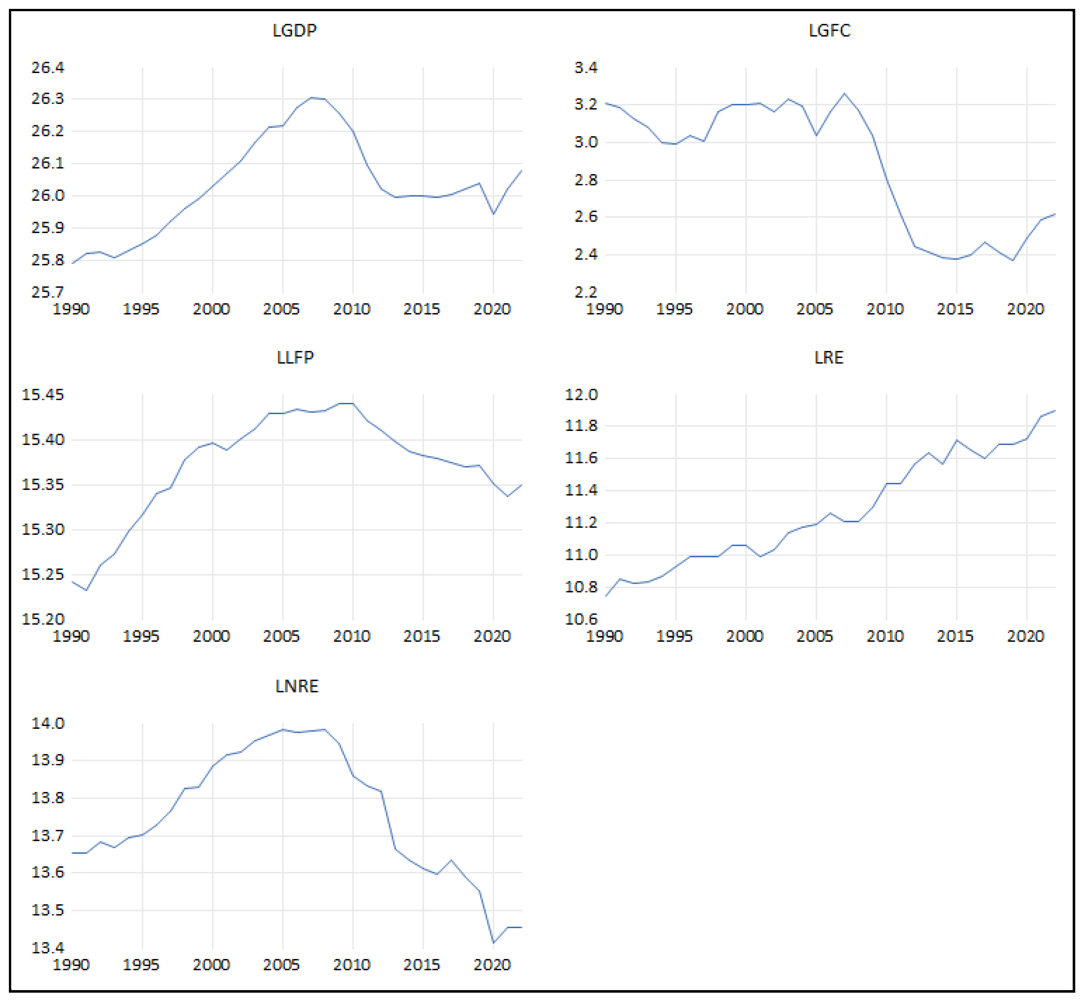
Source: Author’s calculations.

presents the descriptive statistics for the respective variables. The data set consists of 33 observations. Figure 1 shows the graphs of the production variables for the period 1990 to 2022.

From Table 2, we observe that the variable from non-renewable energy sources has a higher average value than the variable from renewable energy sources. This means that the economy and productivity of Greece are dependent on fossil fuels. Furthermore, renewable energy sources, although constantly increasing (see Figure 1), have a secondary role in the economy.

The standard deviation, as is known, measures the extent to which values differ from the average value. The highest deviation value occurs in the production of energy from renewable sources compared to non-renewable sources. This means renewable sources are less stable in the short term, which may make it difficult to completely replace non-renewables without storage technologies (batteries). However, high volatility can also be interpreted as growth momentum. Renewables are growing rapidly, so volatility is naturally higher.

The asymmetry is negative in the production factors of gross fixed capital as a percentage of GDP and the total labor force, with a large negative skewness in the total labor force, and positive in energy sources and production. The greater skewness is in renewable energy sources than in non-renewable sources, indicating that renewable energy sources have a less stable distribution with “bursts” of production. In contrast, non-renewable sources are more symmetrical around their average price, making them more predictable.

A kurtosis value > 3 indicates a more “peaked” distribution with extreme values in the tails, while a kurtosis value < 3 indicates a more “flat” distribution with less extreme values. Of the variables, only the total labor force has a value close to 3, which indicates a mesoconvex distribution. The kurtosis value in renewable energy sources is smaller than that in non-renewable ones. This means that non-renewable sources exhibit higher kurtosis, i.e., more extreme observations (strong fluctuations in fuel prices), while renewable energy sources are stable and balanced compared to non-renewable sources.

Jarque-Bera [32]’s test shows that the series follows a normal distribution.

Figure 1 depicts the variables of model (3) for the period 1990–2022.

From Figure 1, we observe that there is an increasing trend in production until 2007 and then a decline until 2020, before increasing again until the end of the period under consideration. Furthermore, 2007 was the year when the first signs of the global financial crisis appeared. Furthermore, the decline in productivity in 2007 in Greece was due to the fact that the growth model of the previous decade (consumption, lending, and construction) had reached its limits. The economy had not shifted to outward-looking, innovative, and productive sectors, while competitiveness weaknesses were increasing. Thus, as soon as the external “growth levers” slowed down, productivity began to decline.

Gross fixed capital formation as a percentage of GDP shows a stable trend until 2007 and a significant decline until 2019, before increasing until the end of the period. The decline in gross fixed capital formation in 2007 reflects the end of a cycle of over-investment (the Olympic Games and construction) and the inability of the economy to transition to a new production model based on innovation and extroversion.

The total labor force shows an increase until the year 2010 and a decrease in the following years until 2021. The decline in the labor force in Greece after 2010 was the result of a combination of demographic aging, the great economic crisis, which led to youth emigration, unemployment discouragement and early retirement. This created a structural problem in the labor market, reducing the country’s growth potential.

Renewable energy sources show an increasing trend throughout the examined years. Non-renewable energy sources show an increasing trend until 2007 and then a decline until 2020, only to increase slightly thereafter. The steady growth of renewable sources in Greece is mainly due to institutional and political support (EU subsidies) and the reduction in the cost of technologies. On the contrary, the decline of non-renewable sources in 2007 is explained by the combination of high international prices, reduced domestic demand after the Olympic Games and the beginning of the international crisis.

3.3. Preliminary Analysis

Test the Linearity or Nonlinearity of Time Series

To test the linearity or nonlinearity of the series, we use the BDS statistic [33]. The BDS statistic is used as a diagnostic tool to detect nonlinearity and serial dependence of the series. The null hypothesis assumes that the series is independent and identically distributed (i.i.d.), implying linearity and zero serial dependence. The alternative hypothesis indicates nonlinearity or serial dependence.

The BDS statistic essentially consists of using the time lag method to construct an m- dimensional space from the initial time series of length, T. Then, a correlation function is calculated $C_{m,T}(\in )$.

Given a time series, $X_t$, $t=1,2,\dots ,n$, we define a historical point $m$ as $X_t^m=(x_t,x_{t-1},\dots ,x_{t-m+1})$ where the correlation integral at the embedding dimension $m$ is as follows [34]:

$$C_{m,T}(\in )={\displaystyle \sum _{t<s}{I}_{\in }(X_t^m,X_s^m)\left(\frac{2}{T_m(T_m-1)}\right),}$$

(4)

where $T_m=T-(m-1)$, and $I{x}_t^m,x_s^m$ is an indicative function that equals 1 if $‖X_t^m-X_s^m‖<\in$ and 0 otherwise.

Basically, $C_{m,T}(\in )$ measures the increase in the number of $m$ histories that lie within a hypercube of size $\in$ between them. In other words, we would say that the correlation integral estimates the probability of any two $m$ dimension points being at a distance from $\in$ each other [34]:

$$P(\left|X_t-X_s\right|<\in ,\left|X_{t-1}-X_{s-1}<\in ,\dots ,\left|X_{t-m+1}-X_{s-m+1}\right|<\in )\right|.$$

If $X_t$ is iid, this probability should be equal to the following in the limiting case:

$$C_{1,T}{(\in )}^m=P{(\left|X_t-X_s\right|<\in )}^m$$

(5)

Brock [33] defines BDS statistics as follows:

$$V_{m,\in }=\sqrt{T}{\displaystyle \frac{C_{m,T}(\in )-C_{1,T}{(\in )}^m}{s_{m,T}}}$$

(6)

where $s_{m,T}$ is the standard deviation, and it can be estimated consistently [33]. Under fairly moderate normality conditions, the BDS statistic converges to the distribution with N(0, 1).

3.4. Unit Root Testing

3.4.1. Zivot–Andrews Test

Zivot [35], following the form of [36] models, proposes a variation on Perron’s original test in which they assume that the exact time of the break-point is unknown. Taking into account that the break-point is an endogenous phenomenon, Zivot and Andrews propose three models to test for the unit root.

The null hypothesis in all three models is as follows:

$H_0:\widehat{\alpha }=0$, which implies that the series $y_t$ contains a unit root with a shift that excludes any structural break.

The alternative hypothesis is as follows:

$H_1:\widehat{\alpha }<0$, which implies that the series $y_t$ is a trend-stationary process with a one-time break occurring at an unknown point in time.

A. Model with Intercept:

$$y_t={\widehat{\mu }}^A+{\widehat{\vartheta }}^{A}D{U}_t(\widehat{\lambda })+{\widehat{\beta }}^{A}t+{\widehat{\alpha }}^A{y}_{t-1}+{\displaystyle \sum _{j=1}^k{\widehat{\gamma }}_j^A\Delta y_{t-j}+{\widehat{e}}_t}.$$

(7)

B. Model with Trend:

$$y_t={\widehat{\mu }}^B+{\widehat{\beta }}^{B}t+{\widehat{\rho }}^{B}D{T}_t^{\ast }(\widehat{\lambda })+{\widehat{\alpha }}^B{y}_{t-1}+{\displaystyle \sum _{j=1}^k{\widehat{\gamma }}_j^B\Delta y_{t-j}+{\widehat{e}}_t}.$$

(8)

C. Model with Both Intercept and Trend:

$$y_t={\widehat{\mu }}^C+{\widehat{\vartheta }}^{C}D{U}_t(\widehat{\lambda })+{\widehat{\beta }}^{C}t+{\widehat{\rho }}^{C}D{T}_t^{\ast }(\widehat{\lambda })+{\widehat{\alpha }}^C{y}_{t-1}+{\displaystyle \sum _{j=1}^k{\widehat{\gamma }}_j^C\Delta y_{t-j}+{\widehat{e}}_t},$$

(9)

where $D{U}_t$ is a dummy variable for the mean shift and appears in every possible change, whereas $D{T}_t^{\ast }$ is the corresponding variable for the mean shift and trend.

$$D{U}_t\left(\lambda \right)=\left\{\begin{array}{l}1,\hspace{1em}\hspace{1em}\alpha \nu \hspace{1em}\hspace{1em}t>{\rm T}\lambda \\ 0\hspace{1em}\hspace{1em}\hspace{1em}\hspace{1em}otherwise\end{array}\right.,$$

$$D{{\rm T}}_{\tau }^{\ast }\left(\lambda \right)=\left\{\begin{array}{l}t-T\lambda ,\hspace{1em}\hspace{1em}\hspace{1em}\alpha \nu \hspace{1em}t>{\rm T}\lambda \\ 0\hspace{1em}\hspace{1em}\hspace{1em}\hspace{1em}otherwise\end{array}\right..$$

The above models are based on [36]’s models, as a data-dependent algorithm is used as a proxy for Perron to determine the structural points.

3.4.2. Nonlinear Unit Root Test

A nonlinear form that all nonlinear unit root tests use is the nonlinear Exponential Smooth Transition Autoregressive Process (ESTAR) model. The univariate model of the first-order nonlinear Exponential Smoothing Transitional Autoregressive Process (ESTAR) has the following form:

$$y_t=\beta y_{t-1}+\gamma y_{t-1}\left[1-\exp \left\{-\vartheta {\left(s_t-c\right)}^2\right\}\right]+e_t,$$

(10)

where $y_t$ is the series under analysis, $\beta$ and $\gamma$ are unknown parameters, $\vartheta \ge 0$ is the slope parameter and provides the transition speed to the mean inversion, and $e_t\to iid(0,{\sigma }^2)$.

Kapetanios–Shin–Snell (KSS) Unit Root Test

Kapetanios [37] developed a procedure for detecting the presence of non-stationarity against nonlinear but globally stationary exponential smooth transition autoregressive ESTAR processes. For this purpose, they use the following ESTAR model:

$$\Delta y_t=\gamma y_{t-1}\left[1-\exp \left\{-\vartheta y_{t-1}^2\right\}\right]+e_t.$$

(11)

Furthermore, Kapetanios [37] used the first-order Taylor series in Model (11) to obtain the following auxiliary regression:

$$\Delta y_t=\rho y_{t-1}^3+{\displaystyle \sum _{i=1}^k\lambda \Delta y_{t-i}+}{e}_t.$$

(12)

The two assumptions of Equation (12) are written as follows:

$H_0:\rho =0$ (unit root or non-stationary).

$H_1:\rho <0$ (nonlinear stationary ESTAR).

The above hypotheses are tested by the statistic $t_{NL}={\displaystyle \frac{\widehat{\rho }}{s.e.(\widehat{\rho })}}$, where $\widehat{\rho }$ is the estimate of $\rho$ from the auxiliary regression (12).

Kruse Unit Root Test

Kruse [38] extends the unit root test of [37] by allowing the parameter $c\ne 0$ to be non-zero in model (10). Refs. [37,38] used the first-order Taylor series to obtain the following auxiliary regression:

$$\Delta y_t={\delta }_1{y}_{t-1}^3+{\delta }_2{y}_{t-1}^2+{\displaystyle \sum _{j=1}^p{\varphi }_j\Delta y_{t-j}}+e_t.$$

(13)

The two assumptions of Equation (13) are written as follows:

$H_0:{\delta }_1={\delta }_2=0$ (unit root or non-stationary).

$H_1:{\delta }_1<0,{\delta }_2\ne 0$ (nonlinear stationary ESTAR).

The above hypotheses are tested by the statistics $\tau =t_{{\delta }_2^{\perp }=0}^2+1\left({\widehat{\delta }}_1<0\right)t_{{\delta }_1=0}^2$ proposed by [39].

Sollis Unit Root Test

Sollis [40] in Model (10) proposes a control based on an Asymmetric Exponential Smooth Transition Autoregressive (AESTAR) model, where the adaptation speed $\vartheta$ could be different below or above the threshold band. Refs. [37,38,40] used the first-order Taylor series to obtain the following auxiliary regression:

$$\Delta y_t={\varphi }_1{y}_{t-1}^4+{\varphi }_2{y}_{t-1}^3+{\displaystyle \sum _{i=1}^k{k}_i\Delta y_{t-i}+}{\epsilon }_t.$$

(14)

The null hypothesis of Equation (14) is written as follows:

$H_0:{\varphi }_1={\varphi }_2=0$ (unit root or non-stationary).

The above hypothesis is tested with the F statistic, and the critical values are listed in [40]. When the null hypothesis is rejected, the hypothesis $H_0:{\varphi }_2=0$ of the symmetric ESTAR can be tested against the asymmetric AESTAR for $H_0:{\varphi }_2\ne 0$.

3.5. Nonlinear ARDL Approach

The Nonlinear Autoregressive Distributed Lag (NARDL) method is most suitable when the data series exhibit nonlinear relationships and asymmetric behavior. Given the tendency for asymmetry, ref. [7] proposed NARDL as an extension of the conventional ARDL model to capture the long-run impact of the positive and negative effects of the independent variables on the dependent variable. Later, ref. [7] developed a flexible dynamic parametric framework to model relationships that exhibit combined long-run and short-run asymmetries.

In the nonlinear form of the NARDL model, we use the partial sum technique by incorporating the additional variables LRE and LNRE as nonlinear, assuming that they have an asymmetric relationship. We split the variables LRE and LNRE into two other variables, one positive and one negative. This functional dependence captures both the direct and asymmetric effects of positive and negative changes in these variables on the LGDP variable. To operationalize this dependence, the series data were transformed into natural logarithms for two reasons: first, to smooth abrupt fluctuations [41], and second, to make the coefficients interpretable as elasticities.

The mathematical equation of the partial sum procedure is as follows:

$$LR{E}_t^{+}={\displaystyle \sum _{i=1}^t\Delta LR{E}_i^{+}={\displaystyle \sum _{i=1}^t\max (\Delta LR{E}_i,0)}},$$

(15)

$$LR{E}_t^{-}={\displaystyle \sum _{i=1}^t\Delta LR{E}_i^{-}={\displaystyle \sum _{i=1}^t\min (\Delta LR{E}_i,0)}},$$

(16)

$$LNR{E}_t^{+}={\displaystyle \sum _{i=1}^t\Delta LNR{E}_i^{+}={\displaystyle \sum _{i=1}^t\max (\Delta LNR{E}_i,0)}},$$

(17)

$$LNR{E}_t^{-}={\displaystyle \sum _{i=1}^t\Delta LNR{E}_i^{-}={\displaystyle \sum _{i=1}^t\min (\Delta LNR{E}_i,0)}}.$$

(18)

The signs (+) and (−) denote positive and negative changes in the variables LRE and LNRE.

The short-run and long-run relationships between the variables suggested by the Nonlinear Autoregressive Distributed Lag (NARDL) model are provided by the equation:

$$\begin{array}{l}\Delta LGD{P}_t={\delta }_{01}+{\delta }_{11}LGD{P}_{t-1}+{\delta }_{12}LGF{C}_{t-1}+{\delta }_{13}LLF{P}_{t-1}+{\delta }_{14}^{+}LR{E}_{t-1}^{+}+{\delta }_{14}^{-}LR{E}_{t-1}^{-}++{\delta }_{15}^{+}LNR{E}_{t-1}^{+}+\\ {\delta }_{15}^{-}LNR{E}_{t-1}^{-}+{\displaystyle \sum _{i=1}^p{\alpha }_{11i}\Delta LGD{P}_{t-i}+{\displaystyle \sum _{i=0}^{q_1}{\alpha }_{12i}\Delta LGF{C}_{t-i}+{\displaystyle \sum _{i=0}^{q_2}{\alpha }_{13i}\Delta LLF{P}_{t-i}}+}}\\ +{\displaystyle \sum _{i=0}^{q_3}{\alpha }_{14i}^{+}\Delta LR{E}_{t-i}^{+}+{\displaystyle \sum _{i=0}^{q_4}{\alpha }_{14i}^{-}\Delta LR{E}_{t-i}^{-}+}{\displaystyle \sum _{i=0}^{q_5}{\alpha }_{15i}^{+}\Delta LNR{E}_{t-i}^{+}}}+{\displaystyle \sum _{i=0}^{q_6}{\alpha }_{15i}^{-}\Delta LNR{E}_{t-i}^{-}}+{\epsilon }_{1t}\end{array},$$

(19)

where $\Delta$ are the first differences, ${\delta }_{01}$ is the constant term (drift), ${\delta }_{11}$, ${\delta }_{12}$, ${\delta }_{13}$, ${\delta }_{14}^{+}$, ${\delta }_{14}^{-}$, ${\delta }_{15}^{+}$, and ${\delta }_{15}^{-}$ are the long-term coefficients, and ${\alpha }_{11}$, ${\alpha }_{12}$, ${\alpha }_{13}$, ${\alpha }_{14}^{+}$, ${\alpha }_{14}^{-}$, ${\alpha }_{15}^{+}$, ${\alpha }_{15}^{-}$, and ${\epsilon }_{it}$ are the white noise errors (disturbance term). Also, p and q₁, q₂, q₃, q₄, q₅, and q₆ are the maximum time lags of the dependent variables and the independent variables, respectively.

First, we examine the existence of co-integration. The NARDL approach uses the F-Bounds Test [42] to assess co-integration (long-run relationship) between variables. The null hypothesis assumes that there is no long-run relationship. Long-run and short-run asymmetries are examined with the Wald test. The null hypotheses claim that there is no asymmetric relationship between the variables for both the short-run and long-run horizons. Specifically, with the Wald test, we assess long-run co-integration in the asymmetric ARDL approach.

A long-run asymmetric cointegrating relationship exists if the common null hypothesis is $H_0$.

$H_0:{\delta }_{11}={\delta }_{12}={\delta }_{13}={\delta }_{14}^{+}={\delta }_{14}^{-}={\delta }_{15}^{+}={\delta }_{15}^{-}=0$ in Equation (19) is rejected.

Furthermore, if the long-run coefficients

${\displaystyle \frac{-{\delta }_{14}^{+}}{{\delta }_{11}}}\ne 0$, ${\displaystyle \frac{-{\delta }_{14}^{-}}{{\delta }_{11}}}\ne 0$, ${\displaystyle \frac{-{\delta }_{15}^{+}}{{\delta }_{11}}}\ne 0$, and ${\displaystyle \frac{-{\delta }_{15}^{-}}{{\delta }_{11}}}\ne 0$, then there is potential asymmetry in the long run.

Thus, the null hypothesis of a symmetric long-run relationship is as follows:

$${\displaystyle \frac{-{\delta }_{14}^{+}}{{\delta }_{11}}}=0, {\displaystyle \frac{-{\delta }_{14}^{-}}{{\delta }_{11}}}=0, {\displaystyle \frac{-{\delta }_{15}^{+}}{{\delta }_{11}}}=0, {\displaystyle \frac{-{\delta }_{15}^{-}}{{\delta }_{11}}}=0,$$

and it is tested using the Wald statistic following an asymptotic X² distribution.

If $H_0$ is rejected, then there is evidence of long-run asymmetric effects among the variables in the model. Otherwise, these effects are considered symmetric (or linear), so the symmetric ARDL model will be estimated and analyzed based on the estimation results.

3.6. The Asymmetric Causality Test

To test for asymmetric causality, we use [8]’s test. Hatemi-j [8] for asymmetric causality testing considers asymmetries by measuring the combined sums of positive and negative changes in the independent variables. Furthermore, Ref. [8]’s test provides a comprehensive analysis considering not only structural changes but also positive and negative shocks. The results of the test depend on the correct identification of structural changes and shocks. This is an important advantage for understanding short-term and long-term changes in time series data.

Hatemi-J [8] began the investigation of causality between two variables using a random walk proposition. The causal relationship between the two variables is investigated as follows:

$$y_{1t}=y_{1t-1}+{\epsilon }_{1t}=y_{1,0}+{\displaystyle \sum _{Y=1}^t{\epsilon }_{1i}},$$

(20)

$$y_{2t}=y_{2t-1}+{\epsilon }_{2t}=y_{2,0}+{\displaystyle \sum _{Y=1}^t{\epsilon }_{2i}},$$

(21)

where $y_{1t}$ and $y_{2t}$ are two integrated variables. $y_{1,0}$ and $y_{2,0}$ represent the initial values of the variables, and ${\epsilon }_{1i}$ and ${\epsilon }_{2i}$ are the error terms. The above equations show the total shocks defined as follows:

$${\epsilon }_{1i}^{+}=\max ({\epsilon }_{1i},0), {\epsilon }_{1i}^{-}=\min ({\epsilon }_{1i},0),$$

$${\epsilon }_{2i}^{+}=\max ({\epsilon }_{2i},0) {\epsilon }_{2i}^{-}=\min ({\epsilon }_{2i},0).$$

Moreover, ${\epsilon }_{1i}={\epsilon }_{1i}^{+}+{\epsilon }_{1i}^{-}$ and ${\epsilon }_{2i}={\epsilon }_{2i}^{+}+{\epsilon }_{2i}^{-}$.

According to the above vibrations, in Equations (20) and (21), $y_{1t}$ and $y_{2t}$, can be formulated as follows:

$$y_{1t}=y_{1t-1}+{\epsilon }_{1t}=y_{1,0}+{\displaystyle \sum _{Y=1}^t{\epsilon }_{1i}^{+}+{\displaystyle \sum _{Y=1}^t{\epsilon }_{1i}^{-}}},$$

(22)

$$y_{2t}=y_{2t-1}+{\epsilon }_{2t}=y_{120}+{\displaystyle \sum _{Y=1}^t{\epsilon }_{2i}^{+}+{\displaystyle \sum _{Y=1}^t{\epsilon }_{2i}^{-}}}.$$

(23)

In order to capture the asymmetric effects of the variables, the positive and negative shocks of the variables can be calculated as follows:

$$y_{1t}^{+}={\displaystyle \sum _{Y=1}^t{\epsilon }_{1t}^{+}}, y_{1t}^{-}={\displaystyle \sum _{Y=1}^t{\epsilon }_{1t}^{-}}, y_{2t}^{+}={\displaystyle \sum _{Y=1}^t{\epsilon }_{2t}^{+}}, y_{2t}^{-}={\displaystyle \sum _{Y=1}^t{\epsilon }_{2t}^{-}}.$$

Assuming that the equation $y_t^{+}=y_{1t}^{+}+y_{2t}^{+}$ is valid, the causal relationship between the variables $y_{1t}^{+}$ and $y_{2t}^{+}$ is determined using a VAR model with lags “p”, as shown in the equation below:

$$y_t^{+}=v+A_1{y}_{t-1}^{+}+\dots +A_p{y}_{t-p}^{+}+u_t^{+}.$$

(24)

In the above equation, $y_t^{+}$ is a vector of variables of dimensions 2 × 1, $v$ is a vector of intercepts of dimensions 2 × 1, and $u_t^{+}$ is a vector of error terms of dimensions 2 × 1. The table $A_r$ is the 2 × 2 parameter table for lag order $r(r=1,\dots ,p)$. The optimal lag order $p$ is selected by the HJC information for $j=0,\dots ,p$ [43].

$$HJC=\ln (\left|{\widehat{\Omega }}_j\right|)+j\left({\displaystyle \frac{n^2\ln T+2n^2\ln (\ln T}{2T}}\right) j=0,\dots ,p.$$

(25)

The coefficient $\left|{\widehat{\Omega }}_j\right|$ shown in Equation (25) denotes the determinant of the estimation of the variance–covariance index of the error terms in the VAR model, with lag length $j$, n denotes the number of equations in the VAR model, and T denotes the number of observations.

Once the optimal number of lags has been determined, we can define the causality test by forming the null hypothesis as follows:

H0. 

The$kth$ element of $y_t^{+}$ does not Granger-cause the $\mu th$ element of  $y_t^{+}$.

To test for causality, we use the Wald statistic distributed by X². In case the data are not normally distributed, the bootstrap method is used [43].

4. Empirical Results and Discussion

4.1. Linear and Nonlinear Tests (Bds Independence Test)

Table 3. BDS independence test.

BDS Statistic	Dim 2	Dim 3	Dim 4	Dim 5	Dim 6
LGDP	0.161 (0.000)	0.268 (0.000)	0.329 (0.000)	0.362 (0.000)	0.371 (0.000)
LGFC	0.161 (0.000)	0.268 (0.000)	0.322 (0.000)	0.339 (0.000)	0.341 (0.000)
LLFP	0.190 (0.000)	0.318 (0.000)	0.413 (0.000)	0.480 (0.000)	0.519 (0.000)
LRE	0.164 (0.000)	0.268 (0.000)	0.345 (0.000)	0.399 (0.000)	0.434 (0.000)
LNRE	0.153 (0.000)	0.237 (0.000)	0.264 (0.000)	0.276 (0.000)	0.276 (0.000)

Source: Author’s calculations.

presents the results of the BDS test [33] for the independence of the variables LGDP, LGFC, LLFP, LRE, and LNRE. The BDS test detects the nonlinearity of the variables, as well as the serial dependence in time series data. The null hypothesis assumes that the series is linear and independent and identically distributed (i.i.d.). The alternative hypothesis assumes that the series is nonlinear or that the series has serial dependence.

The results of the Table 3 show the rejection of the null hypothesis (significance level less than 1%). Therefore, we can say that there is nonlinearity in the variables, or serial dependence. The test is conducted in increasing dimensions (from Dim 2 to Dim 6), with higher dimensions capturing more complex dependencies. As the BDS statistic increases in higher dimensions, this indicates stronger evidence of nonlinearity or serial dependence, which is observed in all five variables. Rejection of the null hypothesis in all dimensions for each variable confirms the presence of nonlinearity and serial dependence in the data.

The nonlinearity of all variables in the model means that their behavior and their relationship with economic growth are not stable and predictable with simple linear models. Instead, it depends on thresholds, stages of the business cycle, political conditions, and exotic shocks.

Since there is nonlinearity in the variables, we can examine their stationarity with structural change tests, as well as with nonlinear unit root tests. Furthermore, these results suggest the application of the NARDL model as the most appropriate for testing co-integration as it can take into account asymmetries and nonlinearities in the relationships between variables.

4.2. Nonlinear Unit Root Tests

4.2.1. Unit Root Test with Structural Changes

The

Table 4. Unit root test with structural breaks results.

	Zivot–Andrews
	Level
Variables	Intercept	Break	Trend	Break	Intercept and Trend	Break
LGDP	−3.730 *	2010	−3.038	2005	−2.759	2003
LGFC	−4.479 *	2010	−2.492	1999	−3.289	2010
LLFP	−2.400	2011	−3.320	1999	−3.118	1998
LRE	−4.329 *	2010	−3.94 ***	2007	−5.054 *	2010
LNRE	−2.286	1997	−4.318 *	2006	−3.681	2005
	1st difference
Variables	Intercept	Break	Trend	Break	Intercept and Trend	Break
LGDP	−4.896 *	2008	−3.662 **	2013	−5.386 *	2009
LGFC	−4.605 **	2008	−3.988 **	2012	−5.193 *	2008
LLFP	−8.854 *	2016	−6.968 *	2014	−7.530 *	2011
LRE	−4.545 *	2015	−3.320	2013	−3.903 ***	2016
LNRE	−6.046 *	2009	−5.497 *	2014	−6.187 *	2009

*, **, and *** for significance levels 1, 5, and 10, respectively.

provides the results of [35].

The results reported in Table 4 suggest that the time series properties of the examined variables are not uniform and are sensitive to both the type of structural break allowed in the [35] test and the timing of such breaks.

LLFP (Labor Force Participation): The finding that LLFP maintains a unit root across all three [35] specifications (level shift, trend shift, and both) implies that this series follows a non-stationary process even after accounting for a potential endogenous break. In practice, this means shocks to labor force participation are persistent and the variable does not revert to a stable mean or trend. This may reflect the impact of demographic shifts, long-run structural changes in the labor market, or institutional reforms that cannot be captured by a single break adjustment.

LGDP (Gross Domestic Product) and LGFC (Gross Fixed Capital formation): These variables display stationarity only under the level-shift model with a break in 2010, but not under trend-shift or combined models. This is significant: it suggests that the 2008 global financial crisis and its aftermath in 2010 introduced a permanent level adjustment in GDP and investment, but did not fundamentally alter the long-run trend dynamics. The persistence of unit roots in the other model specifications points to fragility in the stationarity claim, meaning that GDP and investment might be better viewed as structurally evolving series that are only weakly mean-reverting once crisis effects are considered.

LRE (Renewable Energy consumption): The fact that this series is stationary in all three forms of [35], with the break located mainly in 2010, is quite telling. It indicates that while renewable energy use has been affected by the structural break (likely due to policy initiatives, EU climate directives, or post-crisis shifts in energy policy), where its dynamics are otherwise mean-reverting. In other words, deviations from the long-run path of renewable energy are temporary and self-correcting, which is consistent with policy-driven stabilization and the gradual integration of renewables into the energy mix.

LNRE (Non-Renewable Energy consumption): The mixed result, stationary only in the trend-shift model but non-stationary in the others, suggests that non-renewables follow a process where the long-run growth trajectory itself has been altered (trend break), rather than a simple level shift. This may capture the structural decline in fossil fuel use after 2010, consistent with rising renewable penetration, changing consumption patterns, and regulatory discouragement of carbon-intensive energy sources. Still, the lack of stationarity in the other forms indicates that shocks to non-renewable energy may have long-lasting effects, reflecting the inertia and slow adjustment of energy systems.

Ref. [35]’s results highlight that 2010 is a critical structural break year across most variables, coinciding with the Greek sovereign debt crisis and broader global financial disruptions, but also aligning with EU energy policy intensification. The mixed stationarity findings imply that while some sectors (like renewable energy) exhibit stability and mean reversion even after structural shocks, others (like labor force participation and non-renewables) are dominated by persistent trends and shocks. For GDP and investment, stationarity is conditional and sensitive to the treatment of breaks, suggesting fragile dynamics that warrant cautious modeling.

4.2.2. Nonlinear Unit Root Tests

In

Table 5. Nonlinear unit root test results.

	$\mathbf{KSS}$ (${\mathit{t}}_{\mathit{N}\mathit{L}}$)		Kruse ($\mathit{\tau }$)		Sollis
Variables	k	Stat	k	Stat	k	${\mathit{H}}_0:{\mathit{\varphi }}_1={\mathit{\varphi }}_2=0$	${\mathit{H}}_0:{\mathit{\varphi }}_2=0$
LGDP	1	0.644	1	5.985	1	1.721	3.044
LGFC	1	−0.995	1	2.765	1	1.209	1.236
LLFP	1	1.030	1	12.24 **	1	6.859 **	12.272 *
LRE	1	1.284	1	1.072	1	5.130 **	4.113 **
LNRE	1	−0.562	1	1.112	1	0.202	0.307

Notes: The symbols * and ** mean the rejection of the null hypothesis of the unit root at 1% and 5%, respectively. KSS: −3.48, −2.93, −2.66; Kruse: 13.75, 10.17, 8.6; Sollis: 6.883, 4.954, 4.157.

, we present the unit root tests on the nonlinear variables.

The results of Table 5 present the results of the statistic $t_{NL}$ obtained from auxiliary regression (12) of [37], the statistic $\tau$ obtained from auxiliary regression (13) of [38], as well as the F statistic obtained from auxiliary regression (14) of [40]. From Table 5, we observe that [37]’s test fails to support the stationarity of all nonlinear ESTAR-type variables. Kruse [38] shows that there is stationarity in the percentage of the labor force in the total population. Sollis [40] reveals that the share of the labor force in the total population and renewable energy sources is nonlinear, stationary, and asymmetric.

The stationary variables of the results in Table 5 mean that, despite the nonlinearities (asymmetries and thresholds), the series tend to return to a long-term equilibrium. Also, the substantive shocks (economic, energy, and institutional) are temporary in nature. Non-stationary variables mean that even with the most flexible, nonlinear approach, the series follows a random walk. Furthermore, shocks have permanent effects, and there is no return to equilibrium.

The results of the unit root tests with structural changes and the nonlinear unit root tests show that the variables are zero-order integral I(0) and first-order integral I(1). The results of the unit root tests and the presence of nonlinearity and serial dependence in the data lead to the NARDL approach, which allows the examination of nonlinear asymmetric and symmetric relationships between variables.

4.3. Co-Integration Analysis Using the NARDL Model

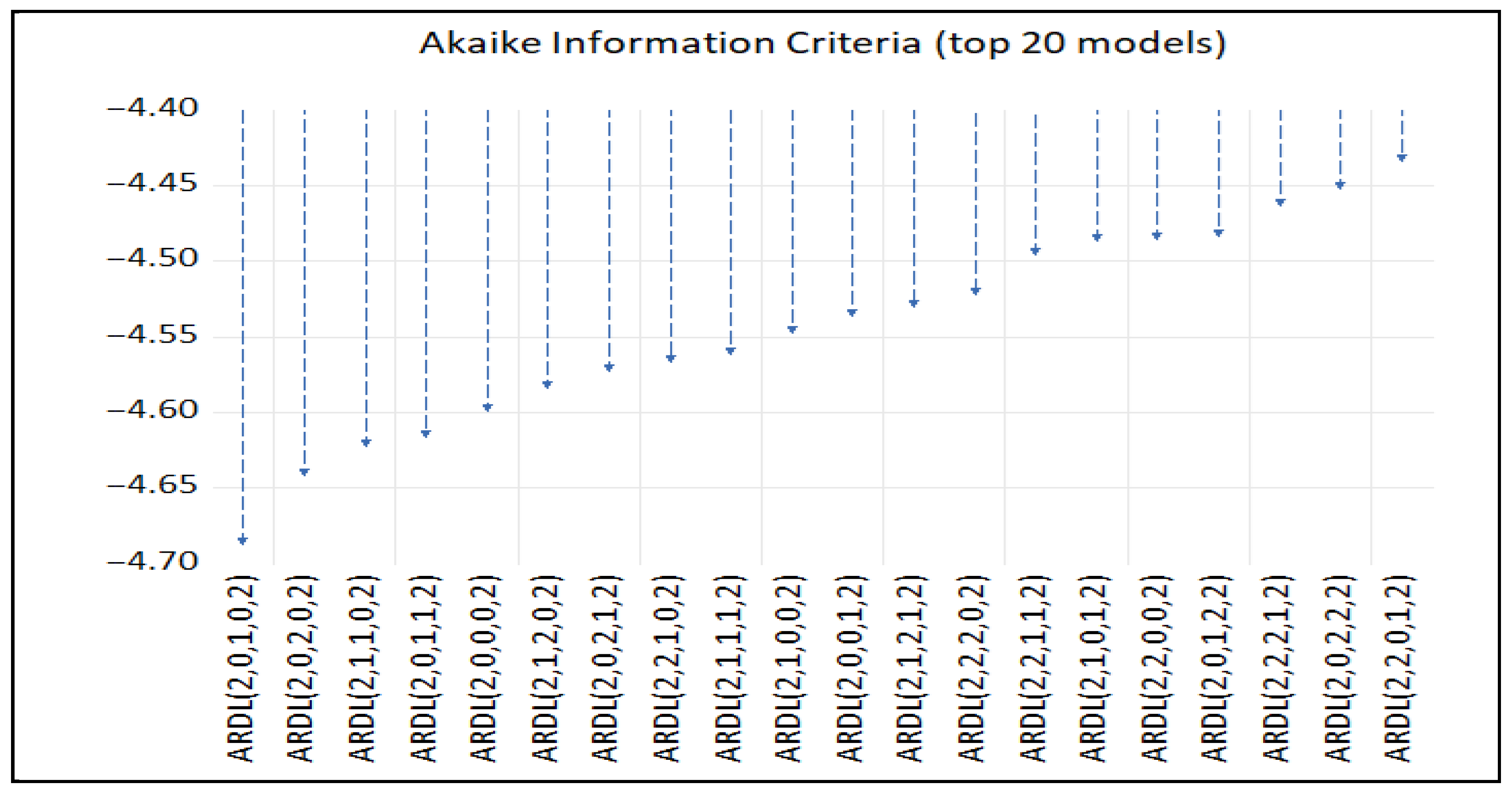
Given these results, the application of the NARDL model is justified, as it can take into account asymmetries and nonlinearities in the relationships between variables. To select the length of the lags for the NARDL model, we use the Akaike Selection Criterion (AIC). The diagram below presents the results from the lags of 20 nonlinear NARDL models. The smallest value of the Akaike criterion gives the optimal lag length of the variables in the nonlinear NARDL model. Similar findings have been provided by SIC and HQIC lag selection criteria.

From Figure 2, the nonlinear model NARDL(2,0,1,0,2) is the most appropriate (it presents the fewest errors). After finding the optimal lag length, we can estimate the nonlinear model NARDL(2,0,1,0,2).

Table 6. Estimation results of the NARDL(2,0,1,0,2) model.

Variable	Coefficient	Std. Error	t-Statistics	Probability
LGDP(−1)	−0.750	0.128	−5.850	0.000
LGFC	0.222	0.047	4.702	0.000
LLFP (−1)	−1.243	0.557	−2.229	0.040
LRE(POS)	0.571	0.157	3.633	0.002
LRE(NEG)	−0.032	0.170	−0.191	0.850
LNRE(−1)(POS)	0.714	0.247	2.883	0.011
LNRE(−1)(NEG)	1.169	0.297	3.926	0.001
C	37.657	9.122	4.127	0.000
DLGDP(−1)	0.590	0.211	2.795	0.013
DLLFP	−0.349	0.710	−0.492	0.629
DLNRE(POS)	0.616	0.399	1.544	0.142
DLNRE(NEG)	0.638	0.144	4.418	0.000
DLNRE(−1)(POS)	−0.158	0.319	−0.496	0.626
DLNRE(−1)(NEG)	−0.678	0.218	−3.106	0.006
Statistics tests
R-squared	0.895	Akaike info criterion	−4.685
Adjusted R-squared	0.809	Durbin–Watson stat	2.361
F-statistic	10.49 (0.00)
Diagnostics tests
			F	Probability
Breusch–Godfrey Serial Correlation LM Test			0.301	0.983
Heteroskedasticity Test: Breusch–Pagan–Godfrey			1.051	0.460
Normality Test: Jarque–Bera			0.289	0.865
Ramsey (RESET)			0.781	0.465

presents the short-run and long-run coefficient estimates of the nonlinear NARDL(2,0,1,0,2) model, with positive and negative shocks occurring in the asymmetric determinants of the renewable and non-renewable energy sources variables (Dependent Variable D(LGDP).

The results in Table 6 show that gross fixed capital as a percentage of GDP contributes positively to the country’s economic growth at the level of 1% in the long run. In contrast, the total labor force contributes negatively to the country’s economic growth at the level of 5%. The results of Table 6 show that increases (positive changes) in renewable energy sources in the long term contribute positively to the country’s economic growth, while conversely decreases (negative changes) have no effect on economic growth. Also, increases (positive changes) in non-renewable energy sources have a positive effect on growth, while decreases (negative changes) in non-renewable energy sources have a negative effect on growth. Here, we should mention that because the coefficient on negative non-renewable sources is greater than that on positive non-renewable sources, we conclude that decreases in the production of non-renewable energy sources have a greater impact on growth than increases in these sources.

From the short-term estimates of the NARDL model in Table 6, we observe that economic growth is not affected by the total labor force, while it is positively affected by the negative change in non-renewable energy sources in the current period and negatively by the negative change in non-renewable energy sources in the previous period at a level of 1%.

Furthermore, the results of both the statistical and diagnostic tests show that there is no problem in the model we are studying. Specifically, the results of the diagnostic tests for the ARDL(2,0,1,0,2) model reveal that there is no problem with autocorrelation, heteroscedasticity, and normality. Meanwhile, the results of the Ramsey (RESET) tests show that there is no error in the specification of the model. Because the results of both the statistical and diagnostic tests do not present any problems, we can proceed to examine the long-term relationship between the variables.

We examine the existence of the long-run cointegrated relationship between the variables of the NARDL(2,0,1,0,2) model by testing the bounds (bound test).

Table 7. The results of the NARDL bound test.

F-Bounds Test		Null Hypothesis: No Linear Relationship
Test Statistic	Value	Sig.	I(0)	I(1)
F-stat.	6.639	10%	2.334	3.515
k	6	5%	2.794	4.148
Sample	30	1%	3.976	5.691

Source: Authors’ estimations.

presents the results of the nonlinear ARDL bound test model for the co-integration of the variables.

The results of Table 7 show that there is a long-term relationship between the variables of the NARDL(2,0,1,0,2) model that we are examining because the calculated F-statistic exceeds all upper critical limits (F = 6.639 > 5.691).

Since there is co-integration between the variables, we can estimate the long-run and short-run relationships of the model NARDL(2,0,1,0,2).

Table 8. Estimation of long-run and short-run coefficients.

Variable	Coefficient	Std. Error	t-Statistics	Probability
Parameters for Long-Run Coefficients (Levels Equation)
LGFC	0.296	0.051	5.828	0.000
LLFP(−1)	−1.656	0.795	−2.082	0.048
LRE(POS)	0.760	0.201	3.775	0.001
LRE(NEG)	−0.043	0.224	−0.193	0.848
LNRE(−1)(POS)	0.951	0.330	2.878	0.008
LNRE(−1)(NEG)	1.558	0.363	4.291	0.000
C	50.170	12.157	4.126	0.000
ECM = LGDP(−1) − (0.296 × LGFC − 1.656 × LLFP(−1) + 0.760 × LRE − 0.043 × LRE + 0.951 × LNRE(−1) + 1.558 × LNRE(−1) + 50.170
Parameters for Short-Run Coefficients (Conditional Error Correction Regression)
ECM(−1) *	−0.750	0.085	−8.738	0.000
DLGDP(−1)	0.590	0.103	5.674	0.000
DLLFP	−0.349	0.336	−1.040	0.308
DLNRE(POS)	0.616	0.173	3.561	0.001
DLNRE(NEG)	0.638	0.082	7.765	0.000
DLNRE(−1)(POS)	−0.158	0.189	−0.836	0.411
DLNRE(−1)(NEG)	−0.678	0.107	−6.288	0.000

Source: Authors’ estimations. Note: * Coefficients derived from ECΜ regression.

presents the long-run and short-run estimates of the coefficients of the NARDL(2,0,1,0,2) model.

The results in Table 8 show that the long-run elasticity coefficients of gross fixed capital as a percentage of GDP are positively related to the production process, while the total labor force is negatively related to the production process at significance levels of 1% and 5%, respectively. Also, from the results of Table 8, it appears that the long-run elasticity coefficients (LNRE⁺ LNRE⁻) associated with the positive and negative shocks occurring in non-renewable energy sources are statistically significant at the 1% level. Additionally, the results show that the long-run elasticity coefficients (LRE⁺) related to the positive shocks occurring in renewable energy sources are statistically significant at the 1% level. Therefore, irregular changes in non-renewable energy sources (both positive and negative shocks) and irregular changes in renewable energy sources (only negative shocks) create potentially asymmetric impacts on the production process in the long run.

This means that regardless of whether non-renewable energy sources increase or decrease, the production process (GDP) is significantly affected in both directions. In other words, we would say that non-renewable energy sources have a two-way causal relationship with the production process. Their increase fuels growth, while their decrease strikes growth. For renewable energy sources, the long-run coefficients are only significant in positive shocks, meaning that when the production of renewable energy sources increases, there is a positive contribution to the production process. However, when there is a reduction (negative shock), there is no significant effect on production. Therefore, we can say that for Greece, the production process is not yet so dependent on renewable energy sources that their reduction would negatively affect it in the long term.

Also, the results in Table 8 show that the short-run elasticity coefficients (LNRE⁻ LNRE⁺) in the current period related to the positive and negative shocks occurring in non-renewable energy sources are statistically significant at the 1% level. In contrast, the short-run elasticity coefficients (LNRE⁻) with a time lag related to negative shocks occurring in non-renewable energy sources are statistically significant at the 1% level. Therefore, we can say that irregular changes in non-renewable energy sources (positive and negative shocks) in the current time period and in (negative shocks) in the period with a time lag create potentially asymmetric impacts on the production process in the short term.

The significant short-term contributions of non-renewable energy sources in the current period mean that changes in non-renewable sources have a direct and strong impact on the production process. Therefore, whether non-renewable sources increase or decrease, the country’s economy responds immediately. In other words, we can say that the country has a high energy dependence on fossil fuels. In addition, the short-term significant coefficients of non-renewable energy sources with a time lag only in negative shocks can be interpreted as indicating that the negative changes (reduction in consumption or production of non-renewable sources) have a delayed negative effect. In other words, we would say that the reduction in the use of non-renewable energy sources does not immediately affect the production process, but the “cost” appears with a delay.

The fact that the coefficients on renewable energy sources are not statistically significant in the short run means that fluctuations in renewable energy sources do not have a measurable or direct impact on the production process. This is because renewable energy sources have a smaller share in the energy mix, so their short-term changes do not affect the production process.

We should also mention here that the short-run elasticity coefficients of gross fixed capital as a percentage of GDP and the short-run elasticity coefficients of the total labor force do not contribute to the production process. Furthermore, we should note that the error correction coefficient is negative and less than unity and statistically significant at the 1% level. Furthermore, the error correction coefficient shows the speed with which the production process adjusts to deviations from the long-run equilibrium. This deviation correction is 75% for each year (fast return).

The presence or absence of asymmetric effects of renewable and non-renewable energy sources on economic growth was investigated using the Wald test on the coefficients of positive and negative shocks of the variables for both the long-term and short-term horizons. The results of the Wald tests are provided in

Table 9. Coefficient symmetry tests.

Null Hypothesis: Coefficient is Symmetric
Variable	Statistic	Value	Probability
Long-run
LRE	F-statistic	7.650	0.013
LΝΡΕ	F-statistic	1.733	0.206
Short-run
LRE	F-statistic	N.A.	N.A.
LΝΡΕ	F-statistic	0.512	0.484

Note: N.A. = Not applicable; short-run coefficients for renewable energy were not statistically significant in the NARDL model.

.

The results in Table 9 show that the model we are examining includes an asymmetric long-run relationship between renewable energy sources and economic growth, but not in the short run. Furthermore, for non-renewable energy sources, the results show that there is a symmetrical relationship with growth in both the long and short terms.

The asymmetric long-term relationship between renewable energy sources means that positive and negative changes in renewable energy sources have different effects on the production process over time. The symmetric long-run relationship between non-renewable energy sources means that positive and negative changes in non-renewable energy sources have a similar effect on the production process in the long run.

In the short-term relationship, there is no effect on renewable energy sources, meaning that in the short term, changes in renewable energy sources do not affect the production process in a statistically significant way. Furthermore, in the short term, the symmetrical relationship between non-renewable energy sources affects the production process in a similar way, either increasing or decreasing.

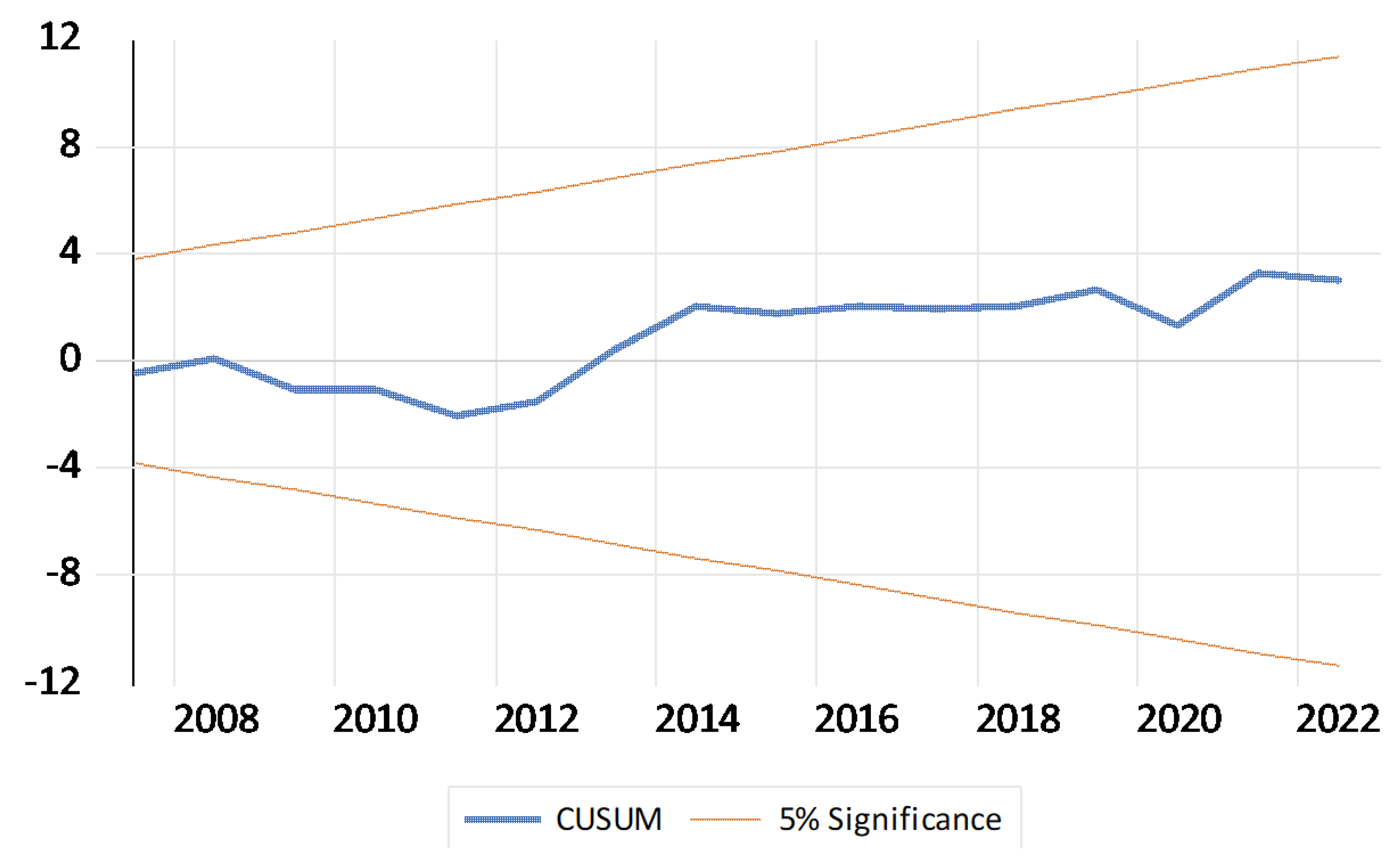
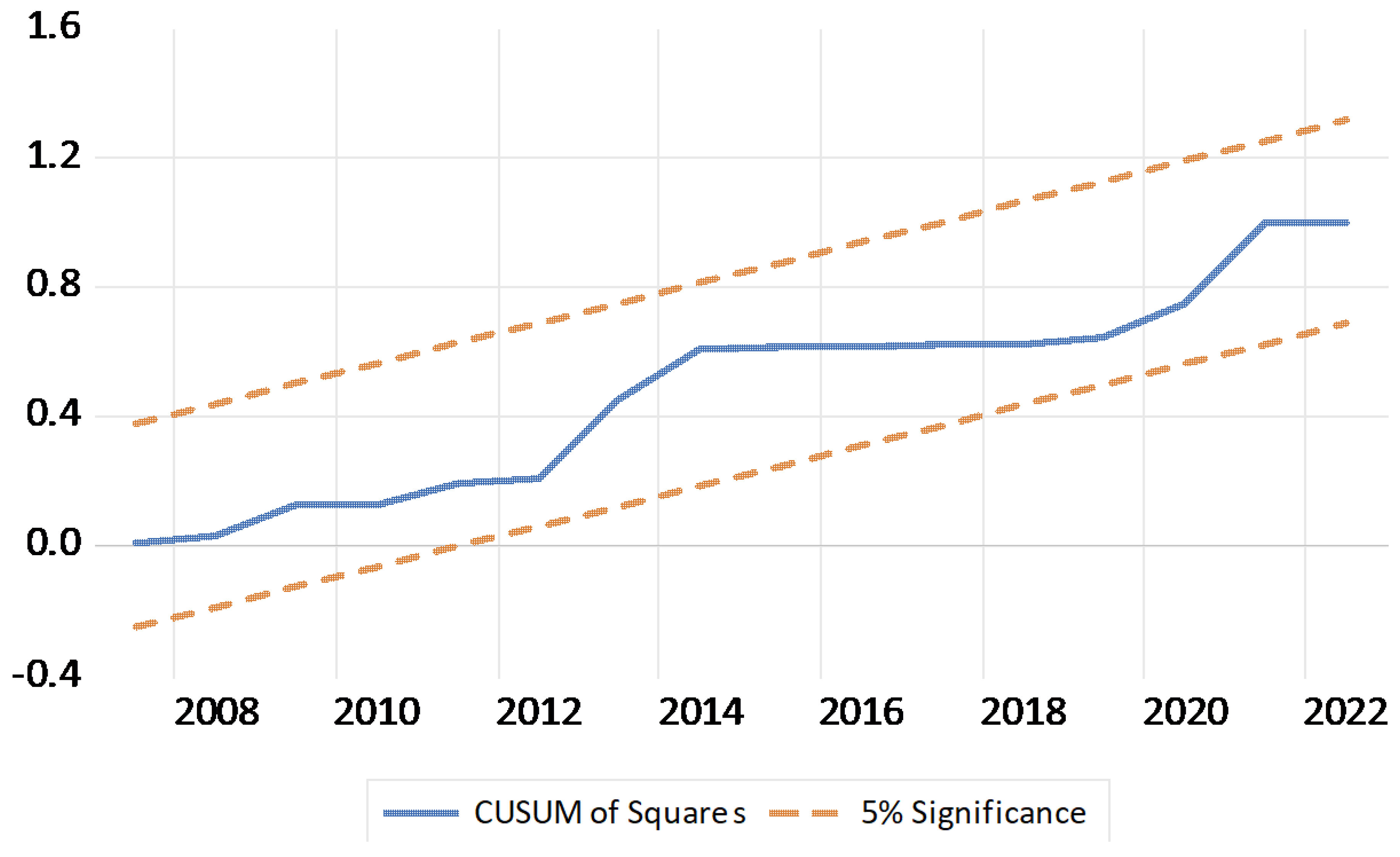
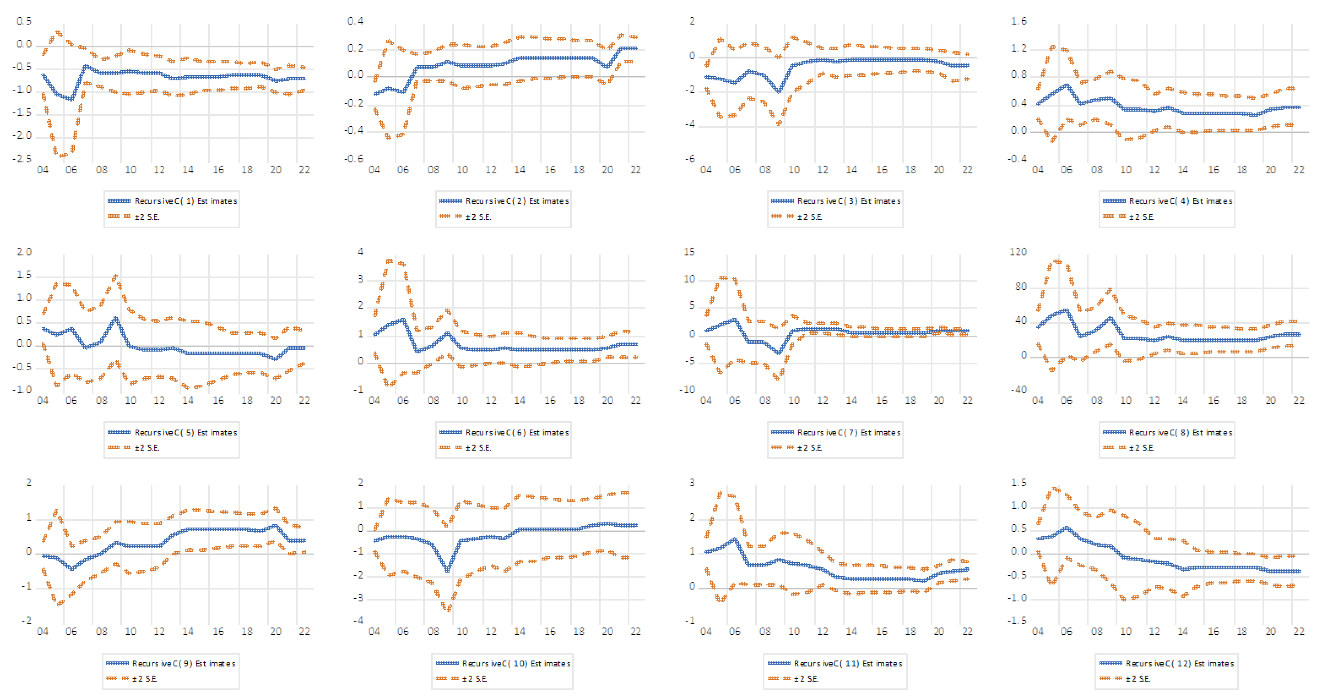
To examine the reliability of the results of the NARDL(2,0,1,0,2) model, we present the CUSUM and CUSUMSQ tests of [44], as well as the recursive coefficients test for the stability of each coefficient of the model. Figure 3 and Figure 4 illustrate the temporal behavior of the sum of the repeated residuals and the sum of the squares of the repeated residuals, respectively and confirm whether the long-term and short-term relationship estimated is stable throughout the period under consideration. Figure 5 illustrates the test of the recursive coefficients of the NARDL(2,0,1,0,2) model.

From the above diagram, we observe that the CUSUM curve remains within the confidence limits. Therefore, we can say that the estimated coefficients in the NARDL model (2,0,1,0,2) are stable throughout the period under consideration, at a significance level of 95%.

From the above diagram, we observe that the CUSUMSQ curve remains within the confidence limits. Therefore, we can say that there are no serious changes in the error variance. Therefore, the NARDL(2,0,1,0,2) model is reliable. This robustness check further highlights that the observed asymmetry is not a byproduct of the chosen lag specification and that the estimated parameters are stable over time, thereby strengthening the validity of the empirical results.

To examine the evolution of the estimates of the regression coefficients on the NARDL(2,0,1,0,2) model data, we use the following diagram. Figure 5 shows the two standard error bands around the estimated coefficients.

From the above diagram, we observe that the estimated values of all coefficients converge to stable levels as the sample size increases. This fact suggests that the NARDL(2,0,1,0,2) model is stable and its estimates are reliable. The small fluctuations observed in some periods do not affect the broader stability. Therefore, we can say that the long-term and short-term relationships estimated by the NARDL(2,0,1,0,2) model consistently reflect the dynamics of the variables.

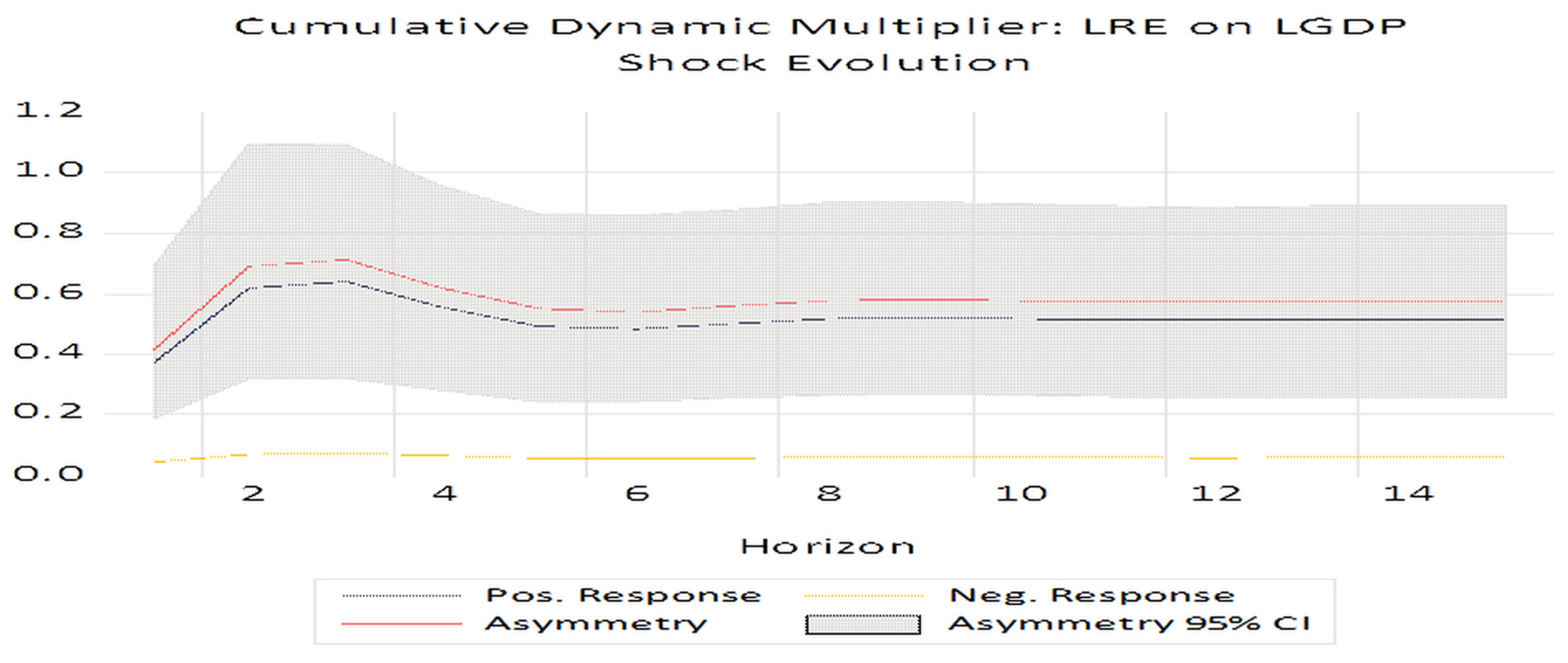
The NARDL model uses Cumulative Dynamic Multipliers (CDMs) to assess the impact of asymmetric changes in the explanatory variables on the dependent variable over time. These multipliers can be positive or negative, reflecting asymmetric effects. The results of the NARDL model confirm the existence of an asymmetric co-integration relationship of renewable energy sources to economic growth. Therefore, cumulative potential multipliers can be used to illustrate the asymmetric responses of renewable energy sources to a change in economic growth. Figure 6 shows the responses of economic growth to changes in renewable energy sources (long-term asymmetry and short-term symmetry).

From Figure 6, we observe that positive shocks from renewable energy sources seem to have a greater impact on economic growth than negative shocks. The difference in impacts seems to be at its maximum in the third year after its occurrence, according to the data in the figure. As shown in Figure 6, the asymmetric impact of renewable energy sources on economic growth is significant in the long run, because the red line marked with “asymmetry” (which shows the impact regardless of whether the change is positive or negative) differs significantly from 0 over the entire period considered. Therefore, we can say that positive changes in renewable energy sources act as a lever for growth (investments, technology, jobs, and environmental benefits). Therefore, their impact is disproportionately greater. Negative changes in renewable energy sources do not have a correspondingly large negative impact because of the following:

• They do not yet have the largest share in the energy mix.
• There are institutional supports (subsidies, long-term contracts).

Table 10. Hatemi-J [43] Asymmetric Causality Test Results.

Null Hypothesis	Wald Test Statistic	p-Value
$LR{E}^{+}$ $\ne$> LGDP	3.467	0.046
$LR{E}^{-}$ $\ne$> LGDP	0.108	0.899
LGDP $\ne$> $LR{E}^{+}$	3.682	0.039
LGDP $\ne$> $LR{E}^{-}$	0.019	0.980

Note: $\ne$> indicates the null hypothesis of no causality.

presents the results of the asymmetric causality test between the variables of renewable energy sources and productive growth.

As can be seen from Table 10, there is a causal relationship between positive shocks to renewable energy sources and economic growth, as well as from economic growth to positive shocks to renewable energy sources. This means that when the production of renewable energy sources increases (a positive shock), this has a causal effect on economic growth. In other words, more “clean” energy leads to higher growth either through

• reducing energy costs;
• increasing investments in new technologies;
• strengthening energy security;
• creating new jobs.

When there is a causal relationship between economic growth and positive shocks in renewable energy sources, it means that increased economic growth causes more positive changes in renewable energy sources. In other words, when the economy grows, demand/investment in renewable energy sources also increases. This can be carried out via the following:

• Higher public and private investments in renewable sources;
• Better technological infrastructure;
• Stricter environmental policies implemented when there is economic comfort.

5. Discussion

The analysis of the asymmetric and nonlinear impacts of renewable and non-renewable energy sources on economic growth in Greece reveals a set of nuanced results with important theoretical and policy implications. First, the persistent higher cost of non-renewable energy relative to renewables during 1990–2022 underscores Greece’s continued structural dependence on fossil fuels. This reliance imposes both economic risks, due to exposure to volatile international markets, and environmental risks, by delaying the transition to sustainability. Despite policy support for renewables, the evidence suggests that the energy mix remains locked into traditional sources-a pattern consistent with “path dependence” in energy systems. From a policy standpoint, this indicates the need for more aggressive diversification measures, including accelerated carbon taxation and strategic reserves, to mitigate exposure to fossil fuel price shocks.

Second, the volatility observed in renewable energy output, reflected in a larger standard deviation and positive skewness, should not be interpreted merely as weakness but as a signal of rapid structural change. The intermittency associated with weather-dependent renewables illustrates both their vulnerability and their growth potential. Critically, this volatility demands complementary investment in storage, smart grids, and balancing technologies. Without these, the short-term inability of renewables to affect growth, as found in the model, is unlikely to change. Thus, technological infrastructure becomes the critical constraint in converting renewable abundance into measurable short-term economic gains.

Third, the higher kurtosis of non-renewable energy sources suggests that fossil fuel dependence exposes Greece to a greater risk of extreme disruptions, often geopolitical in nature. This finding is highly relevant in the current European context, where energy security concerns follow global supply shocks. By contrast, renewables display more stable distributions over time, indicating that, once scaled and integrated, they could provide greater resilience. Policymakers should therefore reframe renewables not just as “green growth” drivers but as stabilizers of macroeconomic and energy security risks in the medium run.

Fourth, the structural breaks observed in 2007 and 2010 highlight the interplay between macroeconomic fragility and the energy–growth nexus. The collapse of the growth model based on consumption, credit, and construction eroded productivity, while the sovereign debt crisis compounded structural labor market weaknesses. These findings caution that energy policy cannot be separated from broader institutional and industrial policy reforms. Energy shocks alone cannot explain productivity decline; rather, they interact with an under-diversified production structure and weak innovation capacity. A coordinated policy mix that links energy transition with labor market renewal, human capital formation, and innovation systems is essential for sustained growth.

The econometric results further highlight important asymmetries in the energy-growth nexus. Positive shocks in renewable energy exert long-term growth-enhancing effects, and, critically, display bidirectional causality with economic growth; meanwhile, negative shocks are absorbed without a measurable impact. This finding signals the presence of endogeneity in the relationship: growth and renewable adoption are mutually reinforcing, rather than operating in a simple one-directional manner. On the one hand, expanding renewable capacity contributes to output through productivity and diversification effects. On the other hand, higher levels of economic growth create the fiscal and financial space for greater investment in renewable technologies, either directly through public spending and subsidies or indirectly through increased private investment and demand for clean energy. This cyclical dynamic implies that the two variables cannot be treated as strictly exogenous to one another, and standard linear models that assume unidirectional causality risk misattributing effects or underestimating feedback loops.

From a policy perspective, this endogenous feedback loop has both opportunities and risks. During periods of sustained growth, the cycle can generate momentum by attracting new investment into renewables, fostering technological innovation, and further reinforcing growth. However, in downturns or crises, the same mechanism can operate in reverse: weaker growth may constrain investment flows into renewables, slowing the energy transition and increasing reliance on fossil fuels. The asymmetry observed in our results, where negative renewable shocks have no significant growth impact, may currently reflect the small share of renewables in the energy mix and the cushioning effect of subsidies. Yet, as the renewable share expands, the potential for downturn-induced slowdowns in clean energy investment could become more pronounced. The implication is that policies must not only support upward trajectories of renewable adoption but also de-risk renewable investment during downturns, for example, through countercyclical public investment, green bonds, or EU-level stability mechanisms.

By contrast, non-renewable energy demonstrates symmetric effects in both the short and long run, with positive shocks fostering growth and negative shocks impeding it. Here, the absence of asymmetry suggests that fossil fuel dependence exposes the Greek economy to proportionate impacts in both directions, amplifying its vulnerability to international market volatility. This symmetry illustrates the fundamental fragility of the current growth model, where reliance on non-renewables ensures that any fluctuation, positive or negative, directly affects output. Reducing this symmetric dependence through accelerated substitution toward renewables thus becomes not merely a climate imperative but a macroeconomic stability strategy.

Finally, the broader lesson is that Greece’s energy-growth nexus is characterized by asymmetric transition dynamics: fossil fuels remain the binding constraint in the short run, while renewables exert asymmetric growth benefits only in the long run. Policy should therefore operate on two complementary fronts: (i) short-term resilience policies to buffer fossil fuel price volatility (e.g., hedging strategies, emergency reserves, and diversification of import sources), and (ii) long-term innovation-oriented policies that scale renewables, invest in storage and grid integration, and align subsidies with productivity-enhancing sectors. Linking these energy policies to human capital and industrial upgrading is essential if renewables are to evolve from a politically supported sector into a genuine driver of sustainable growth.

6. Conclusions

This study explored the asymmetric and nonlinear effects of renewable and non-renewable energy sources on Greece’s economic growth from 1990 to 2022, utilizing an extended Cobb–Douglas production function and the NARDL model. The findings reveal that non-renewable energy sources have significant short- and long-term impacts on growth, with both positive and negative shocks exerting strong effects, underscoring Greece’s continued dependence on fossil fuels. In contrast, renewable energy contributes positively to growth only in the long term, with increases in renewables stimulating growth but decreases having no equivalent negative effect, reflecting their still-limited role in the energy mix. Asymmetric causality results show a bidirectional link between renewable energy expansion and economic growth, suggesting a virtuous cycle where growth encourages green investments, while negative renewable shocks remain neutral due to stabilizing policies and their supplementary role in the energy system. The results highlight the need for accelerated diversification away from fossil fuels through investment in renewable infrastructure, storage, and smart grids. Policymakers should promote countercyclical financing instruments, such as green bonds, to maintain renewable investment during downturns. Integrating energy policy with industrial innovation and human capital development can amplify the long-term growth benefits of renewables. Fiscal incentives and regulatory frameworks should be adaptable to evolving market maturity and technology diffusion. Ultimately, Greece’s sustainable growth strategy must treat the energy transition not only as an environmental priority but as a cornerstone of economic resilience and competitiveness

References

1. Persis, J.; Ben Amar, A. Predictive modeling and analysis of air quality-Visualizing before and during COVID-19 scenarios. J. Environ. Manag. 2023, 327, 116911. [Google Scholar] [CrossRef]
2. Dritsaki, M.; Dritsaki, C.; Argyriou, V.; Sarigiannidis, P. Impact of renewable and non-renewable generation on economic growth in Greece. Electr. J. 2024, 37, 107421. [Google Scholar] [CrossRef]
3. Stern, D.I. Energy use and economic growth in the USA: A multivariate approach. Energy Econ. 1993, 15, 137–150. [Google Scholar] [CrossRef]
4. Apergis, N.; Payne, J.E. Renewable energy consumption and economic growth: Evidence from a panel of OECD countries. Energy Policy 2010, 38, 656–660. [Google Scholar] [CrossRef]
5. Ozturk, I. A literature survey on energy–growth nexus. Energy Policy 2010, 38, 340–349. [Google Scholar] [CrossRef]
6. Payne, J.E. Survey of the international evidence on the causal relationship between energy consumption and growth. J. Econ. Stud. 2010, 37, 53–95. [Google Scholar] [CrossRef]
7. Shin, Y.; Yu, B.; Greenwood-Nimmo, M. Modelling asymmetric co-integration and dynamic multipliers in a nonlinear ARDL framework. In Festchrift in Honor of Peter Schmidt: Econometric Methods and Applications; Horrace, W., Sickles, R., Eds.; Springer: New York, NY, USA, 2014; pp. 281–314. [Google Scholar] [CrossRef]
8. Hatemi-J, A. Asymmetric causality tests with an application. Empir. Econ. 2012, 43, 447–456. [Google Scholar] [CrossRef]
9. Sari, R.; Soytas, U. The growth of income and energy consumption in six developing countries. Energy Policy 2007, 35, 889–898. [Google Scholar] [CrossRef]
10. Ruhul, S.; Kamrul, H.; Sahar, S. Renewable and non-renewable energy consumption and economic activities: Further evidence from OECD countries. Energy Econ. 2014, 44, 350–360. [Google Scholar] [CrossRef]
11. Dergiades, T.; Martinopoulos, G.; Tsoulfidis, L. Energy consumption and economic growth: Parametric and non-parametric causality testing for the case of Greece. Energy Econ. 2013, 36, 686–697. [Google Scholar] [CrossRef]
12. Inglesi-Lotz, R. The impact of renewable energy consumption to economic growth: A panel data application. Energy Econ. 2016, 53, 58–63. [Google Scholar] [CrossRef]
13. Pegkas, P. Energy consumption and human capital: Does human capital stimulate renewable energy? The Case of Greece. J. Knowl. Econ. 2024, 15, 17256–17283. [Google Scholar] [CrossRef]
14. Halicioglu, F.; Ketenci, N. Output, Renewable and Non-Renewable Energy Production, and International Trade: Evidence from EU-15 Countries. MPRA 2018, 87621. Available online: https://mpra.ub.uni-muenchen.de/87621 (accessed on 20 July 2025).
15. Okumus, İ.; Guzel, A.E.; Destek, M.A. Renewable, Non-Renewable Energy Consumption and Economic Growth Nexus in G7: Fresh Evidence from CS-ARDL. MPRA 2022, 114136. Available online: https://mpra.ub.uni-muenchen.de/114136 (accessed on 15 March 2025).
16. Triantafyllidou, A.; Polychronidou, P.; Mantzaris, I. Primary energy consumption and economic growth: The case of Greece. East. J. Eur. Stud. 2023, 14, 108–132. [Google Scholar] [CrossRef]
17. Afzal, A.; Hasnaoui, J.; Noor, R.; Banerjee, A. Is saving the non-renewable resources worthwhile? Evidence of paradox of plenty on human capital development. Resour. Policy 2023, 83, 103728. [Google Scholar] [CrossRef]
18. Hoa, P.X.; Xuan, V.N.; Thu, N.T.P. Determinants of the renewable energy consumption: The case of Asian countries. Heliyon 2023, 9, e22696. [Google Scholar] [CrossRef]
19. Hashemizadeh, A.; Abadi, F.Z.B.; Fan, C. Geopolitical perspective on global renewable energy development considering China’s technological and Belt & Road scenarios. Renew. Energy 2025, in press. [Google Scholar]
20. Cobb, C.W.; Douglas, P.H. A theory of production. Am. Econ. Rev. 1928, 18, 139–165. Available online: https://www.aeaweb.org/aer/top20/18.1.139-165.pdf (accessed on 12 May 2025).
21. Behera, J.; Mishra, A.K. Renewable and non-renewable energy consumption and economic growth in G7 countries: Evidence from panel autoregressive distributed lag (P- ARDL) model. Int. Econ. Econ. Policy 2020, 17, 241–258. [Google Scholar] [CrossRef]
22. Shastri, S.; Mohapatra, G.; Giri, A.K. Economic growth, renewable and nonrenewable energy consumption nexus in India. Int. J. Energy Sect. Manag. 2020, 14, 777–792. [Google Scholar] [CrossRef]
23. Zafar, M.W.; Shahbaz, M.; Hou, F.; Sinha, A. From nonrenewable to renewable energy and its impact on economic growth: The role of research & development expenditures in Asia-Pacific Economic Cooperation countries. J. Clean. Prod. 2019, 212, 1166–1178. [Google Scholar] [CrossRef]
24. Polat, B. The impact of renewable and nonrenewable energy consumption on economic growth: A dynamic panel data approach. Asia-Pac. J. Account. Econ. 2021, 28, 592–603. [Google Scholar] [CrossRef]
25. Asif, M.; Bashir, S.; Khan, S. Impact of non-renewable and renewable energy consumption on economic growth: Evidence from income and regional groups of countries. Environ. Sci. Pollut. Res. 2021, 28, 38764–38773. [Google Scholar] [CrossRef] [PubMed]
26. Zhang, X.; Zhang, X. Nexus among economic growth, carbon emissions, and renewable and non-renewable energy in China. Environ. Sci. Pollut. Res. 2021, 28, 39708–39722. [Google Scholar] [CrossRef]
27. Khan, I.; Zakari, A.; Ahmad, M.; Irfan, M.; Hou, F. Linking energy transitions, energy consumption, and environmental sustainability in OECD countries. Gondwana Res. 2022, 103, 445–457. [Google Scholar] [CrossRef]
28. Dogan, E. Analyzing the linkage between renewable and non-renewable energy consumption and economic growth by considering structural break in time-series data. Renew. Energy 2016, 99, 1126–1136. [Google Scholar] [CrossRef]
29. Sikic, T.F. The impact of energy consumption on economic growth in developed and post-transition countries of European Union. Zb. Rad. Ekon. Fak. Rijeci 2020, 38, 475–497. [Google Scholar] [CrossRef]
30. The World Bank. World Development Indicators [Data Set]. 2024. Available online: https://databank.worldbank.org/source/world-development-indicators (accessed on 15 March 2025).
31. BP. Statistical Review of World Energy 2023, 72nd ed.; BP/Energy Institute: London, UK, 2023. [Google Scholar]
32. Jarque, C.M.; Bera, A.K. Efficient tests for normality, homoscedasticity and serial independence of regression residuals. Econ. Lett. 1980, 6, 255–259. [Google Scholar] [CrossRef]
33. Brock, W.A.; Dechert, W.; Scheinkman, J. A Test for Independence Based on the Correlation Dimension; Working Paper; University of Winconsin at Madison: Madison, WI, USA; University of Houston: Houston, TX, USA; University of Chicago: Chicago, IL, USA, 1987. [Google Scholar]
34. Bisaglia, L.; Gerolimetto, M. Testing for (Non)Linearity in Economic Time Series: A Monte Carlo Comparison; Working Paper Series 3; University of Padua: Padua, Italy, 2014. [Google Scholar]
35. Zivot, E.; Andrews, K. Further evidence on the great crash, the oil price shock, and the unit root hypothesis. J. Bus. Econ. Stat. 1992, 10, 251–270. [Google Scholar] [CrossRef]
36. Perron, P. The great crash, the oil price shock, and the unit root hypothesis. Econometrica 1989, 57, 1361–1401. [Google Scholar] [CrossRef]
37. Kapetanios, G.; Shin, Y.; Snell, A. Testing for a unit root in the nonlinear STAR framework. J. Econom. 2003, 112, 359–379. [Google Scholar] [CrossRef]
38. Kruse, R. A new unit root test against ESTAR-based on a class of modified statistics. Stat. Pap. 2011, 52, 71–85. [Google Scholar] [CrossRef]
39. Abadir, K.M.; Distaso, W. Testing joint hypotheses when one of the alternatives is one-sided. J. Econom. 2007, 140, 695–718. [Google Scholar] [CrossRef]
40. Sollis, R. A simple unit root test against asymmetrical STAR nonlinearity with an application to real exchange rates in Nordic Countries. Econ. Model. 2009, 26, 118–125. [Google Scholar] [CrossRef]
41. Lütkepohl, H.; Xu, F. The role of the log transformation in forecasting economic variables. Empir. Econ. 2012, 42, 619–638. [Google Scholar] [CrossRef]
42. Pesaran, M.H.; Shin, Y.; Smith, R.J. Bounds testing approaches to the analysis of level relationships. J. Appl. Econom. 2001, 16, 289–326. [Google Scholar] [CrossRef]
43. Hatemi-J, A. A new method to choose optimal lag order in stable and unstable VAR models. Appl. Econ. Lett. 2003, 10, 135–137. [Google Scholar] [CrossRef]
44. Brown, R.L.; Durbin, J.; Evans, J. Techniques for testing the constancy of regression relationships over time. J. R. Stat. Soc. Ser. B 1975, 37, 149–192. [Google Scholar] [CrossRef]
Figure 1. Time series graphs of variables graphs.
Energies 18 05394 g001
Figure 2. Lag selection criteria for the NARDL model using AIC.
Energies 18 05394 g002
Figure 3. CUSUM test for the estimated NARDL model.
Energies 18 05394 g003
Figure 4. CUSUMSQ test for the estimated NARDL model.
Energies 18 05394 g004
Figure 5. Recursive coefficients test for the estimated NARDL model.
Energies 18 05394 g005
Figure 6. Cumulative dynamic multiplier.
Energies 18 05394 g006