The Influence of the Cu-Al₂O₃ Ratio of the Receiving Tube in a 50 MW Hybrid Solar Plant

Abstract

Direct steam generation (DSG) is a promising technology for introducing solar energy into industrial applications, yet it still faces significant challenges. This work analyzes two critical issues associated with DSG: temperature gradients on the receiver tube wall caused by direct and concentrated radiation and flow instability resulting from the phase transition of the working fluid from liquid–vapor to vapor. These phenomena can reduce the mechanical strength of the receiver tube and lead to sudden pressure increases, deformation, or rupture, which hinder the implementation of DSG in solar thermal plants. To address these challenges, the behavior of a receiver tube composed of copper on the inside and an Al₂O₃ envelope is studied. A 50 MWe hybrid solar thermal plant is proposed for Mulegé, Baja California Sur, Mexico, including a solar field designed to analyze the production of superheated steam during peak solar irradiance hours. The effect of the Cu-Al₂O₃ ratio on the receiver tube is evaluated, with Al₂O₃ serving as a thermal regulator to reduce temperature gradients and mitigate flow instability. This combination of materials improves the receiver tube’s performance, ensuring mechanical stability and enhancing the viability of DSG systems. By reducing temperature gradients and flow instability, DSG-based plants can double thermal efficiency and significantly lower environmental impact by eliminating the need for thermal oils, which require frequent replacement. These findings demonstrate the potential for hybrid solar thermal plants to provide sustainable and efficient solutions for industrial energy needs.

1. Introduction

Hybrid solar plants are designed to address various environmental and social problems, thus contributing to the transition toward more sustainable energy systems [1]. Solar technologies are integrated with other renewable-energy sources or storage systems to reduce dependence on fossil fuels, thus reducing greenhouse gas emissions as well as mitigating climate change and its environmental impact. This not only offers direct environmental benefits but also fosters broader awareness concerning the importance of sustainable-energy solutions [2,3].

Advances in the design of these plants [4] have resulted in the development of programmable electronic systems to monitor environmental parameters and manage electrical functions in solar thermal plants. In a previous study, a control unit was designed to acquire data from temperature and light sensors, process information, and control external devices (pumps, electric valves, and power supplies) to improve plant performance, maximize efficiency, and achieve energy savings.

Direct steam generation (DSG), which is a parabolic trough solar technology, uses a parabolic trough concentrator that focuses solar energy on each receiving tube to generate steam and drive a power-generation system. DSG offers the advantages of low operating cost and high thermal efficiency as it does not require additional heat exchangers and does not lose a significant amount of heat when heat is transferred from thermal oil to steam [5,6,7,8]. However, owing to the possibility of uneven flow distributions and other instabilities related to liquid–vapor flow in parallel pipelines, DSG technology has not been adopted for commercial applications. Various studies pertaining to the instability of two-phase flows in vertical pipes have been conducted [9,10,11,12,13,14]. In the nuclear industry, two-phase flows in parallel pipes are of great interest because of the instability that occurs in boiling-water reactors and loss-of-cooling accidents. Instability problems such as pressure drop oscillations, density wave oscillations, and flow paths have been discussed comprehensively; consequently, useful conclusions have been obtained, which have been practically applied in engineering [15]. The instability of two-phase flows in horizontal pipes is governed primarily by the relationship between fractional pressure drop and flow rate.

Ref. [16] performed a detailed thermoeconomic analysis on a solar thermal plant applied to greenhouses. The main objective was to technically and economically evaluate a well composed of gravel and water that was strategically located in a greenhouse to utilize the available space therein. The analysis was distinguished by its original focus on the loading and unloading phases over one year of operation based on the effective hourly heating demand and actual meteorological data. In the study, sensitivity analysis was performed to determine the levelized cost of heat by considering key variables such as the solar-collector area and storage-well volume. The results revealed the possibility of a design solution with minimum costs that can fulfill 100% of the heat demand, with an estimated levelized heat cost of 153.3 EUR/MWh. These findings highlight the economic viability of thermal energy storage systems as an effective option for mitigating the environmental impact of greenhouses. In this study, a hybrid solar thermal plant is investigated numerically to evaluate the effect of the Cu-Al₂O₃ ratio in the receiving tube on the working fluid.

Simulations and numerical analyses of solar thermal systems are essential for understanding complex processes as well as for energy, economic, and environmental evaluations. In this study, a hybrid solar thermal plant is investigated numerically to evaluate the Cu-Al₂O₃ ratio effects in receiving tubes on system performance. This work presents five fundamental contributions:

• The development of system architecture and plant design introduces a 50 MWe hybrid solar thermal facility for Mulegé, Mexico. The design establishes operational parameters (380 °C, 100–117 bar), methods for solar field sizing, and optimal configuration with 87 loops of six concentrators each. This base design provides the foundation for subsequent analyses.
• A Cu-Al₂O₃ composite wall receiver tube combines thermal conductivity from copper with stability from alumina in a 50–50 ratio. Numerical analysis demonstrates that this configuration reduces pressure drop by 3.3% compared to pure alumina tubes while maintaining structural integrity. The composite design balances thermal efficiency with mechanical stability.
• The characterization of flow dynamics identifies and models three distinct regions within receiver tubes: preheating, evaporation, and superheating. The analysis develops two-phase flow pressure drop models and methods for analyzing stratified flow patterns, establishing critical relationships between solar irradiance and flow instability magnitude.
• Heat transfer modeling presents mathematical frameworks describing interactions between composite materials and working fluid. The models incorporate angle-dependent boundary conditions and thermal interface behavior, characterizing thermal contact resistance and expansion effects at material interfaces.
• The integrated mathematical framework encompasses all aspects of system design and operation. This includes equations for solar field sizing, mass and energy conservation models, and correlations for geometric and thermal properties. The numerical results validate the proposed models and demonstrate that mechanical instabilities primarily affect the copper portion, while thermal instabilities impact the alumina portion of the composite wall.

The remainder of this article is structured as follows: Section 2 introduces the hybrid solar plant design and describes key system components, with an emphasis on the Cu-Al₂O₃ composite receiver tubes. Section 3 presents the solar field sizing methodology and theoretical framework, including radiation distribution analysis. Section 4 develops the mathematical models for flow regions and instabilities in the receiving tube, while Section 5 establishes the heat transfer analysis in the composite wall. Section 6 presents numerical results focusing on thermal and mechanical instability effects in different regions of the composite receiver tube. Finally, Section 7 provides conclusions and implications for future solar thermal plant designs.

2. System Description of Hybrid Solar Plant

This study proposes the installation of a hybrid solar thermal plant with direct steam generation of 50 MW_e, as shown in Figure 1, in Mulegé, Baja California Sur, Mexico. This site features high solar potential and is in a remote area, which cannot access electricity supplied by the national power grid [17].

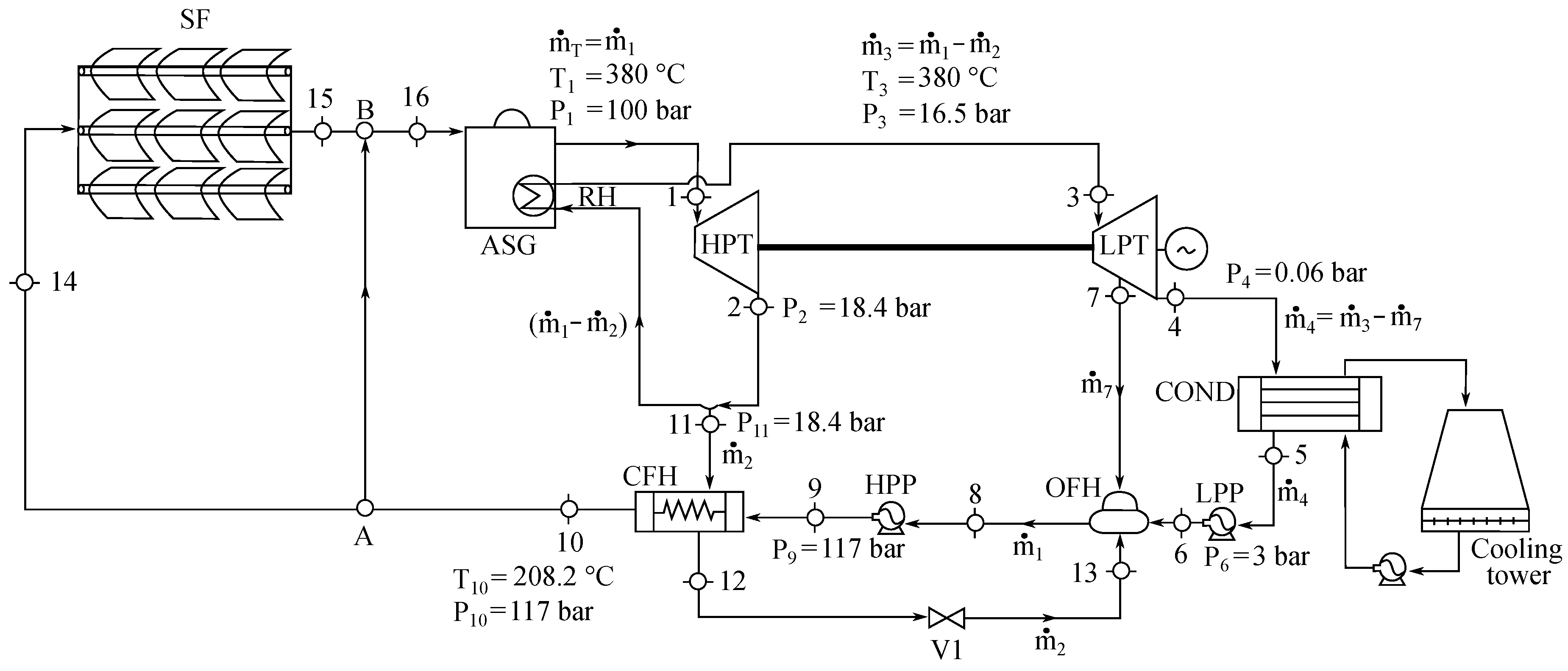
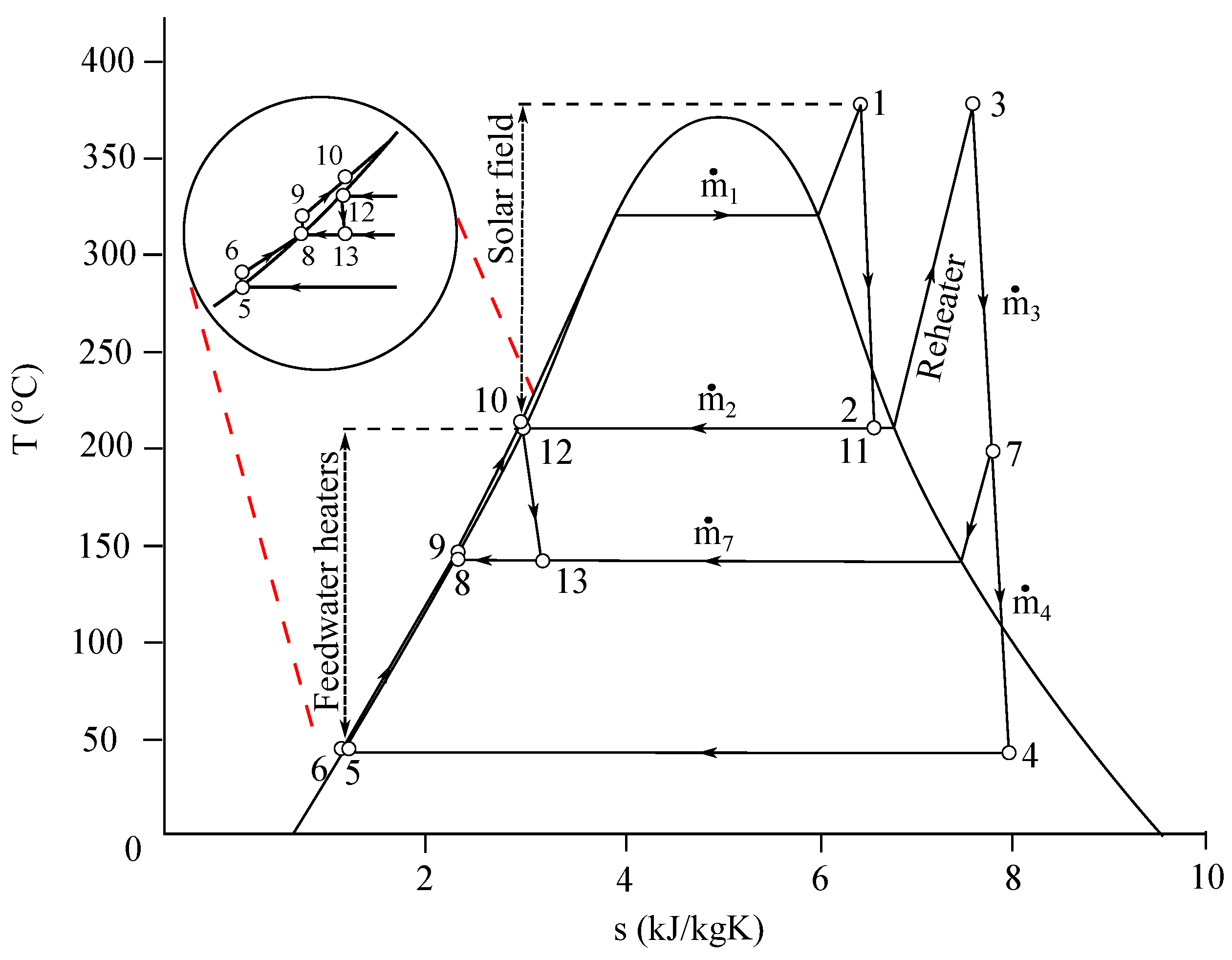
The hybrid solar thermal power plant (see Figure 1) features an SF that operates during the solar irradiance interval to produce superheated steam, which is used as input to the high-pressure turbine (HPT) of the power cycle. The solar field concentrator loops operate in the single-pass mode [18]. During periods of solar intermittency or absence, the flow from the SF is extracted from wet steam to superheated steam (SHS) via an auxiliary boiler (ASG) to achieve the conditions required in the HPT (#1). The auxiliary boiler in the proposed hybrid solar plant operates during periods of insufficient solar irradiance, specifically activating after 16:00 and deactivating at 10:00 the following day. Its role is critical to maintaining continuous electricity production, ensuring the financial viability of the plant even without thermal storage systems. While the auxiliary boiler does not directly impact the overall thermal efficiency of the plant, its integration allows for a stable output by compensating for variations in solar energy availability. This design choice highlights the importance of hybrid configurations in balancing renewable energy integration with consistent power generation. The wet steam exiting the HPT is reheated in the reheater (RH) to reach the SHS at a temperature of 380 °C via the combustion of natural gas (#2 to #3) and then input to the low-pressure turbine (LPT) (#3). The wet vapor exiting the LPT is condensed in a condenser (COND) (#4) to obtain water in a saturated liquid state (#5). The pressure of this liquid-water flow is increased through its passage through the low-pressure pump (LPP) to obtain compressed liquid water (#6), thus preventing counterflow between the currents originating from the extraction of the LPT (#7) and closed heater (CFH) (#12). To reduce the dimensions of the SF, steam extractions are performed in the HPT (#11) and LPT (#7) to preheat the liquid-water flows supplied to the SF in the CFH and open heaters (OFHs), respectively. The pressure of the water flowing out of the OFH increases to that required by the SF (in this case, 117 bar) in the high-pressure pump (HPP) (#9). To satisfy the temperature requirements of the water upon entry into the SF, the flow of water exiting the HPP (#9) is heated in the CFH (#10).

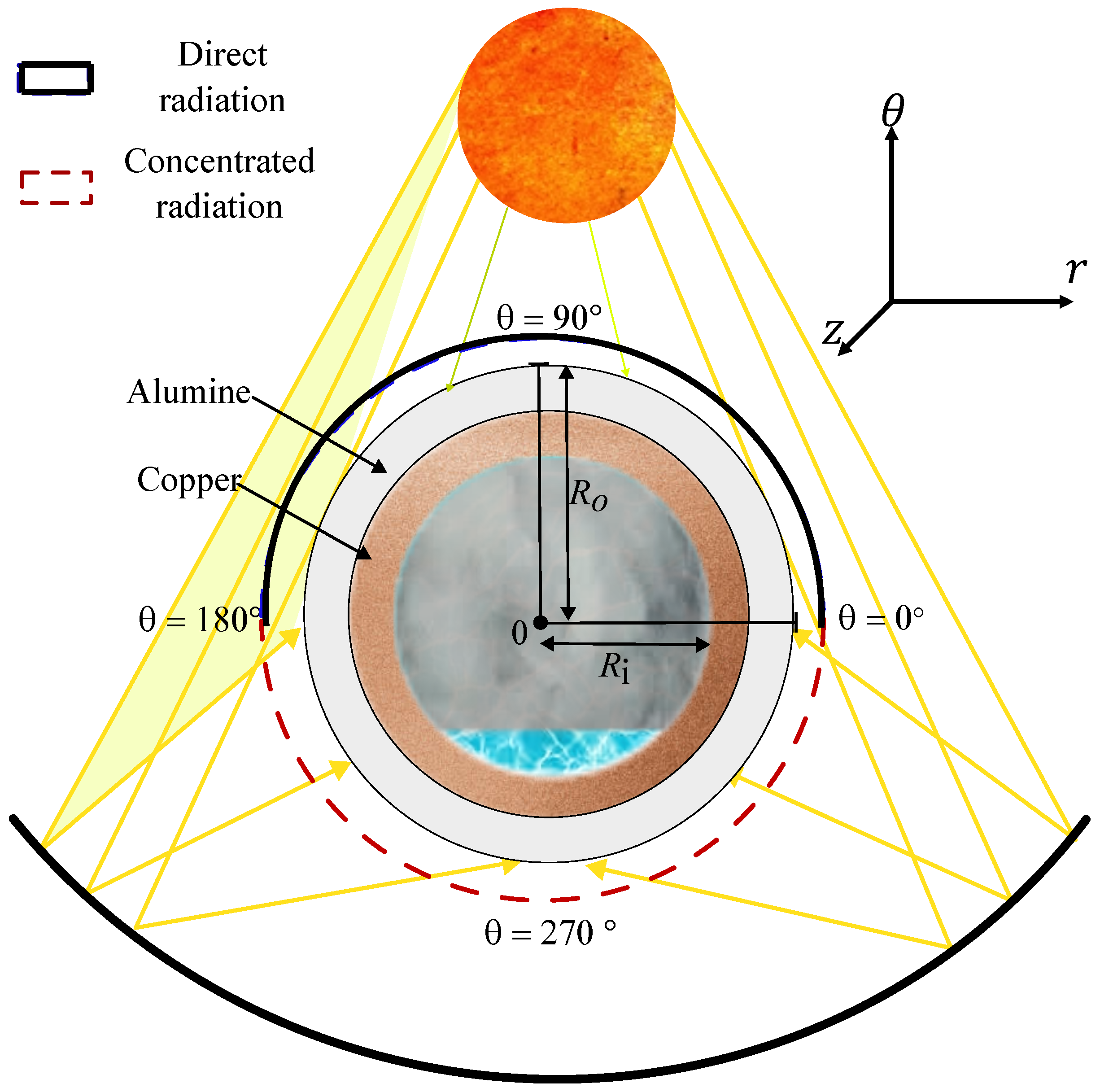
Meanwhile, the function of a parabolic trough solar concentrator is to capture and concentrate solar irradiance on its surface and subsequently reflect it on the lower external wall of the receiving tubes. The irradiance received by the receiver is calculated using the geometric concentration ratio, $R_{\mathrm{c}}$, which is the ratio of the collection areas of the receiving tube $A_{\mathrm{CTR}}$ to the area of the concentrator parabola $A_{\mathrm{P}}$.

$$\begin{array}{c}\hfill R_{\mathrm{c}}={\displaystyle \frac{A_{\mathrm{CTR}}}{A_{\mathrm{P}}}}\end{array}$$

(1)

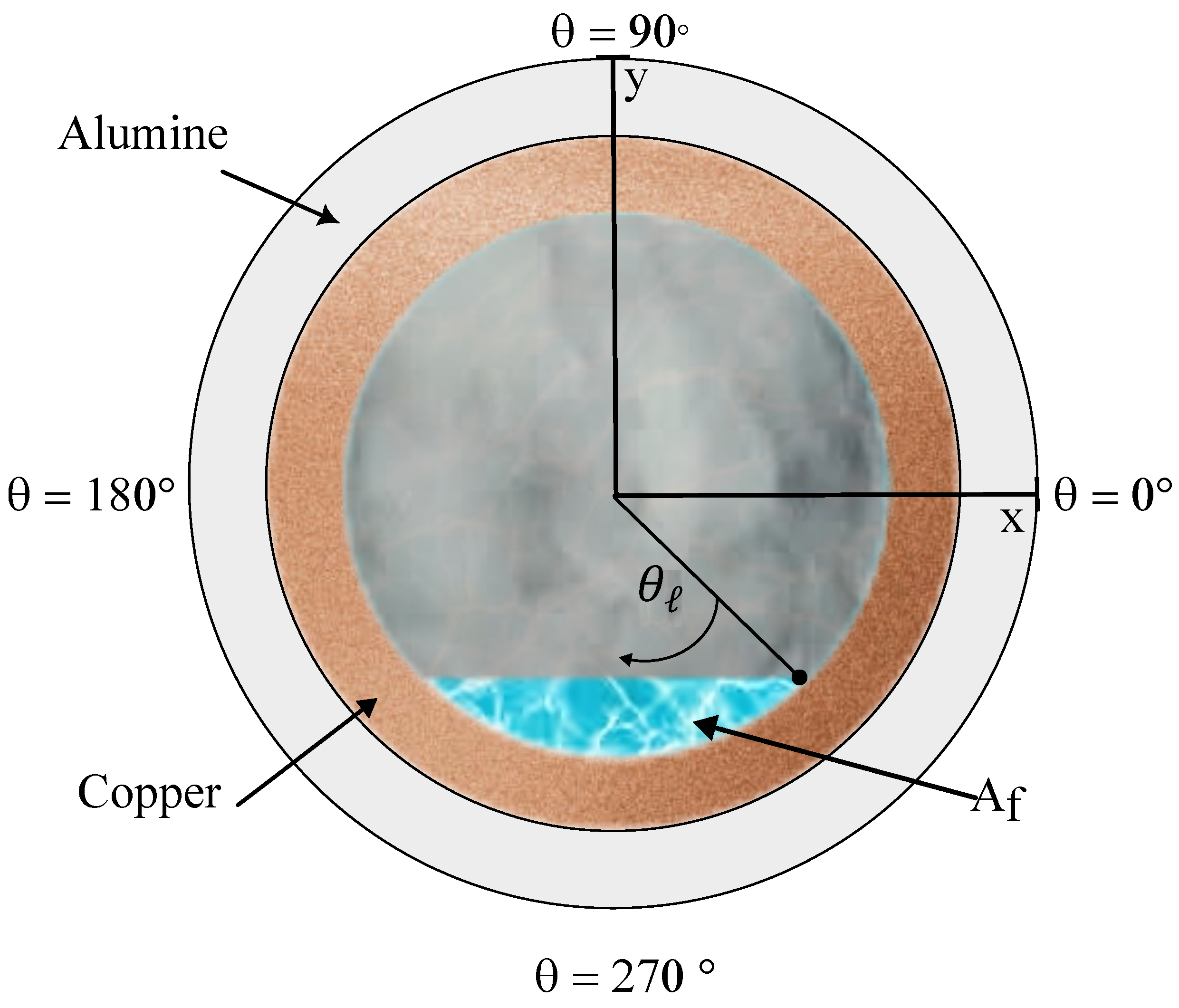
Figure 2 shows the cross-section of the composite wall receiving tube, where $R_{\mathrm{o}}$ is the outer radius of the alumina, $R_{\mathrm{i}}$ the inner radius of the copper, and $\theta$ the opening angle. In this case, direct and concentrated contributions are considered in the upper ($0^{\circ }<\theta <{180}^{\circ }$) and other regions (${180}^{\circ }<\theta <{360}^{\circ }$) of the wall of the alumina receiving tube, respectively. In other words, for $\theta \in 0^{\circ },{180}^{\circ }$, the solar radiation is normal and uniform, and for $\theta \in {180}^{\circ },{360}^{\circ }$, the radiation originates from the surface of the concentrator. In this case, the radiation in the concentrator is 24.8 times greater than that received at the top.

3. Sizing of SF for Hybrid Solar Plant

An SF is an extensive area where devices designed to capture solar energy are installed for conversion to heat. Therefore, an SF can vary in size and configuration depending on its specific purpose. Based on [18,19,20,21], the following assumptions in this study are introduced:

• The optical and thermal efficiencies of the collection equipment are 80% and 70%, respectively;
• The collector fouling factor is F_S = 95% and the interception factor F_I = 98%;
• The length of the collector is 150 m, the opening measures 5.77 m, and the geometric concentration ratio is 82.1;
• The length of the receiving tube is 150 m, the external diameter is 70 mm, and the internal diameter is 65 mm;
• The operation mode is single-step;
• In the evaporation region, the working fluid exhibits a stratified flow pattern;
• The design parameters are the temperatures and pressures of the liquid water at the entrance to the SF, i.e., $T_{10}=208.2$ °C and $P_{10}=117$ bar, and at the exit, i.e., $T_1=380$ °C and $P_1=100$ bar.

3.1. Power Plant

For the power plant, its operation was established in a steady state. Meanwhile, the thermodynamic properties of water were determined using the Xsteam water software (https://xsteam.sourceforge.net/). The isentropic efficiency of the turbines and pumps was 85%, the equipment was operated adiabatically, and changes in the kinetic and potential energy were disregarded [22,23,24]. Thus, the design parameters were as follows:

• Temperature and pressure of the superheated steam at the inlet of the HPT: $T_1=380$ °C and $P_1=100\mathrm{bar}$;
• Temperature and pressure of the superheated steam at the inlet of the LPT: $T_3=380$ °C and $P_3=16.5$ bar;
• Pressure and temperature at the outlet of the COND: $P_5=0.06$ bar and $T_5=T_{\mathrm{sat}@P_5}$;
• Temperature and pressure at the outlet of the CFH: $T_{10}$ = 208.2 °C and $P_{10}$ = 117 bar;
• Pressure at the outlet of the LPP: $P_6=3$ bar;
• Pressure at the outlet of the HPP: $P_8=117$ bar;
• Steam-extraction pressure in the HPT: $P_2=18.4$ bar;
• Steam-extraction pressure in the LPT: $P_7=3$ bar.

3.2. Non-Uniform Radiation Distribution to Size SF

To determine the solar field distribution of the hybrid solar thermal plant in Mulegé, Mexico, the operating conditions of the Andasol 1 solar thermal plant, which is located in Granada, Spain, were considered for reference and corrected based on the environmental conditions of the proposed site [18,25,26]. The field solar concentrator loop comprised six concentration systems, each measuring 150 m long and connected in series, with a total extension of 925 m. The receiving tubes featured an external diameter of 7 m and a Cu-Al₂O₃ composite wall, as shown in Figure 2.

The distribution of daily direct solar irradiance, $G_{\mathrm{bn}}$, for the geographical coordinates of Mulegé (27°4′00.2″ N 112°1′00.2″ O), was obtained from the database of the Photovoltaic Geographic Information System of the European Union [27], where the solar irradiance on the collection surface was obtained using an east–west tracking system. To operate an SF, the direct irradiance of solar tracking must exceed 400 W/m². This requirement, although satisfied in the summer, is not satisfied in the winter because of reduced solar hours. Hence, if the steam conditions required by the HPT are not satisfied in the SF, then the ASG must be operated as shown in the diagram in Figure 1.

The horizontal direct solar irradiance, $G_{\mathrm{bh}}$, which affects the collection surface of the solar concentrator, was obtained by correcting the normal direct irradiance $G_{\mathrm{bn}}$ of the study site with the zenith angle ${\theta }_{\mathrm{z}}$:

$$G_{\mathrm{bh}}=G_{\mathrm{bn}}cos{\theta }_{\mathrm{z}}$$

(2)

The zenith angle of the sun, ${\theta }_z$, correlates the position of the sun in the sky with the latitude of the observation site and the solar time of the day, according to [28]:

$$\begin{array}{ccc}\hfill cos\left({\theta }_{\mathrm{z}}\right)=sin\left(\varphi \right)·sin\left(\delta \right)+cos\left(\varphi \right)·cos\left(\delta \right)·cos\left(\omega \right)& \hfill & \hfill {\theta }_{\mathrm{z}}\in 0°,90°,\end{array}$$

(3)

where $\varphi$ is the latitude of the observation location; $\delta$ is the solar declination, which is the position of the sun on the eclipse; and $\omega$ is the solar hour angle, which represents the position of the sun on its daily path. In this case, the highest position of the sun with respect to the plane of the equator is the maximum value that the decline can reach, i.e., ${\delta }_{\max }={23.45}^{\circ }$. The decline is estimated as a function of ${\delta }_{\max }$ and the natural number of days in a year, $n_{\mathrm{N}}$, using the Cooper approximation [21]:

$$\delta ={\delta }_{\max }sin\left[{\displaystyle \frac{(284+n_{\mathrm{N}})360}{365}}\right]$$

(4)

Meanwhile, the hour angle is the angular displacement of the sun throughout the day with respect to the zenith angle normal to the surface and changes in $15°$ every hour. Negative and positive values of the hour angle were recorded before and after noon, respectively, and the maximum value was obtained at noon, based on the following equation:

$$\omega ={15}^{\circ }(\mathrm{hour}-12)$$

(5)

The incidence of direct solar irradiance on the collection surface, as recorded using the solar tracking system, was obtained using the following expression [21]:

$$G_{\mathrm{bT}}=G_{\mathrm{bh}}\sqrt{1-{cos}^2\delta {sin}^2\omega }$$

(6)

where $G_{\mathrm{bT}}$ is the solar irradiance captured by the tracking system, which affects the collection surface of the concentrator loop in the axial direction. Ref. [29] modeled irradiance as a function of the z position of the concentrator loop while considering a non-uniform normal distribution.

$$G_{\mathrm{bT}}\left(z\right)=G_{\mathrm{bT},\max }{exp}^{-0.27{(z-0.5)}^2},$$

(7)

where $G_{\mathrm{bT},\max }$ is the maximum irradiance incident on the collection system at a specific time of the day.

3.3. Power Cycle Thermal Energy Requirement

The flow of water and heat required by the SF to generate 50 MW_e of power was determined by the mass and energy balances in each of the plant components. Next, expressions were obtained for the mass flows of water and their properties in thermodynamic states, which were determined based on the design parameters of the power cycle, as listed in

Table A1. Properties of water in thermodynamic states of hybrid solar plant.

State	P	T	h	s	Region	$\dot{\mathit{m}}$
1	$P_1$	$T_1$	$h_{1@P_1,T_1}$	$s_{1@P_1,T_1}$	SHS$@P_1,T_1$	${\dot{m}}_1$
2s	$P_2$	$T_{2s@P_2,s_{2s}}$	$h_{2s@P_2,s_{2s}}$	$s_{2s}=s_1$	${\displaystyle \frac{s_{2s}-s_{f@P_2}}{{\left(s_{fg}\right)}_{@P_2}}}$	${\dot{m}}_{2s}={\displaystyle \frac{{\dot{m}}_1(h_{10}-h_9)}{h_{11}-h_{12}}}$
2	$P_2$	$T_{2@P_2,h_2}$	$h_2=h_1-{\eta }_{\mathrm{SIT}}\left(h_1-h_{2s}\right)$	$s_{2@P_2,h_2}$	$x_{2@P_2,h_2}$	${\dot{m}}_2={\dot{m}}_{2s}$
3	$P_3$	$T_3$	$h_{3@P_3,T_3}$	$s_{3@P_3,T_3}$	SHS$@P_3,T_3$	${\dot{m}}_3={\dot{m}}_1-{\dot{m}}_2$
7s	$P_7$	$T_{7s@P_7,s_{7s}}$	$h_{7s@P_7,s_{7s}}$	$s_{7s}=s_3$	SHS$@P_7,s_{7s}$	${\dot{m}}_{7s}={\displaystyle \frac{{\dot{m}}_1{h}_8+{\dot{m}}_4{h}_6-{\dot{m}}_2{h}_{13}}{h_7}}$
7	$P_7$	$T_{7@P_7,h_7}$	$h_7=h_3-{\eta }_{\mathrm{sic}}\left(h_3-h_{7s}\right)$	$s_{7@P_7,h_7}$	SHS$@P_7,h_7$	${\dot{m}}_7={\dot{m}}_{7s}$
4s	$P_4$	$T_{4s@P_4,s_{4s}}$	$h_{4s@P_4,s_{4s}}$	$s_{4s}=s_7$	$x_{4s@P_4,h_{4s}}$	${\dot{m}}_4={\dot{m}}_3-{\dot{m}}_7$
4	$P_4$	$T_{4@P_4,h_4}$	$h_4=h_7-{\eta }_{\mathrm{sic}}\left(h_7-h_{4s}\right)$	$s_{4@P_4,h_4}$	$x_{4@P_4,h_4}$	${\dot{m}}_4$
5	$P_5=P_4$	$T_{5@P_5,x_5}$	$h_{5@P_5,x_5}$	$s_{5@P_5,x_5}$	$x_5=0$	${\dot{m}}_5={\dot{m}}_4$
6s	$P_6=P_7$	$T_{6s@P_6,s_{6s}}$	$h_{6s@P_6,s_{6s}}$	$s_{6s}=s_5$	CL$@P_6,s_{6s}$	${\dot{m}}_{6s}={\dot{m}}_5$
6	$P_6$	$T_{6@P_6,h_6}$	$h_6=h_5+{\displaystyle \frac{h_{6s}-h_5}{{\eta }_{\mathrm{SIB}}}}$	$s_{@P_6,h_6}$	CL$@P_6,s_6$	${\dot{m}}_6={\dot{m}}_5$
8	$P_8=P_6$	$T_{8@P_8,x_8}$	$h_{8@P_8,x_8}$	$s_{8@P_8,x_8}$	$x_8=0$	${\dot{m}}_8={\dot{m}}_1$
9s	$P_9$	$T_{9s@P_9,s_{9s}}$	$h_{9s@P_9,s_{9s}}$	$s_{9s}=s_8$	CL$@P_9,s_{9s}$	${\dot{m}}_9={\dot{m}}_8$
9	$P_9$	$T_{9s@P_9,h_9}$	$h_9=h_8+{\displaystyle \frac{h_{9s}-h_8}{{\eta }_{\mathrm{SIB}}}}$	$s_{@P_9,h_9}$	CL$@P_9,s_9$	${\dot{m}}_9={\dot{m}}_8$
10	$P_{10}=P_9$	$T_{10}=T_{sat@P_{10}}+TTD$	$h_{@P_{10},T_{10}}$	$s_{10@P_{10},T_{10}}$	CL$@P_{10},s_{10}$	${\dot{m}}_1$
11	$P_{11}=P_2$	$T_{11}=T_2$	$h_{11}=h_2$	$s_{11}=s_2$	$x_{11}=x_2$	${\dot{m}}_2$
12	$P_{12}=P_{11}$	$T_{12@P_{12},x_{12}}$	$h_{12@P_{12},x_{12}}$	$s_{12@P_{12},x_{12}}$	$x_{12}=0$	${\dot{m}}_2$
13	$P_{13}=P_7$	$T_{13@P_{13},h_{13}}$	$h_{13}=h_{12}$	$s_{13@P_{13},h_{13}}$	$x_{13@P_{13},h_{13}}$	${\dot{m}}_2$

.

The water–vapor extractions in the HPT and LPT, which are used to preheat the water flow entering the SF in the OFH and CFH, correspond to the extraction curves shown in the T–s power cycle diagram in Figure 3. The heat flow ${\dot{Q}}_{\mathrm{sum}}$ supplied to the power cycle is the sum of the flows in the RH, ${\dot{Q}}_{\mathrm{sum},\mathrm{RH}}$, and through the SF, ${\dot{Q}}_{\mathrm{sum},\mathrm{SF}}$ (see Figure 1), or

$$\begin{array}{c}\hfill {\dot{Q}}_{\mathrm{sum}}=\underset{{\dot{m}}_1\left(h_1-h_2\right)}{\underbrace{{\dot{Q}}_{\mathrm{sum},\mathrm{SF}}}}+\underset{{\dot{m}}_3(h_3-h_7)+{\dot{m}}_4(h_7-h_4)}{\underbrace{{\dot{Q}}_{\mathrm{sum},\mathrm{RH}}}}\end{array}$$

(8)

The global energy balance of the power cycle is expressed as

$$\begin{array}{c}\hfill \dot{W}=\underset{{\dot{m}}_1(h_1-h_2)+{\dot{m}}_3(h_3-h_7)+{\dot{m}}_4(h_7-h_4)}{\underbrace{{\dot{Q}}_{\mathrm{sum}}}}-\underset{{\dot{m}}_1\left(h_9-h_8\right)+{\dot{m}}_4\left(h_8-h_6\right)}{\underbrace{{\dot{Q}}_{\mathrm{rech}}}}\end{array}$$

(9a)

$$\begin{array}{c}\hfill \dot{W}={\dot{m}}_1(h_1-h_2)+{\dot{m}}_3(h_3-h_7)+{\dot{m}}_4(h_7-h_4)\end{array}$$

(9b)

$$\begin{array}{c}\hfill -\left[{\dot{m}}_1\left(h_9-h_8\right)+{\dot{m}}_4\left(h_8-h_6\right)\right]\end{array}$$

(9c)

Based on the balance of Equations (8) and (9a), the motor work generated is obtained as follows:

$$w_m={\displaystyle \frac{\dot{W}}{{\dot{m}}_1}}=(h_1-h_2-h_9+h_8)+{\displaystyle \frac{{\dot{m}}_3}{{\dot{m}}_1}}(h_3-h_7)+{\displaystyle \frac{{\dot{m}}_4}{{\dot{m}}_1}}(h_7-h_4-h_8+h_6)$$

(10)

Subsequently, the generated steam flow ${\dot{m}}_1$ is expressed as

$$\begin{array}{c}\hfill {\dot{m}}_1={\displaystyle \frac{\dot{W}}{w_m}}={\displaystyle \frac{\dot{W}}{(h_1-h_2-h_9+h_8)+\frac{{\dot{m}}_3}{{\dot{m}}_1}(h_3-h_7)+\frac{{\dot{m}}_4}{{\dot{m}}_1}(h_7-h_4-h_8+h_6)}}\end{array}$$

(11)

The useful thermal power of the concentrator, ${\dot{Q}}_{\mathrm{u},\mathrm{conc}}$, is the difference between the effective irradiance that affects the collector and the thermal power losses of the concentration system.

$${\dot{Q}}_{\mathrm{u},\mathrm{conc}}=A_{\mathrm{c}}{\eta }_{\mathrm{op}}{\eta }_{\mathrm{th}}{\mathrm{F}}_{\mathrm{S}}{\mathrm{F}}_{\mathrm{I}}{G}_{\mathrm{bT}}-U_{\mathrm{loss},\mathrm{abs}}{A}_{\mathrm{abs}}\left(T_{\mathrm{abs}}-T_{\mathrm{amb}},\right)$$

(12)

where $A_{\mathrm{c}}$ is the collection area; ${\eta }_{\mathrm{op}}$ is the optical efficiency of the collector; ${\eta }_{\mathrm{th}}$ is the thermal efficiency of the receiving tube; $A_{\mathrm{abs}}$ is the area of the receiving tube; $T_{\mathrm{abs}}$ is the average surface temperature of the receiving tube; $T_{\mathrm{amb}}$ is the ambient temperature; and $U_{\mathrm{loss},\mathrm{abs}}$ is the global loss coefficient, which corresponds to the thermal power losses of the concentration system [30],

$$U_{\mathrm{loss},\mathrm{abs}}={\displaystyle \frac{1}{\frac{R_{\mathrm{o}}}{R_{\mathrm{i}}{h}_{\alpha }}+\frac{R_{\mathrm{o}}}{k_{\alpha }}ln\frac{R_{\mathrm{o}}}{R_{\mathrm{i}}}}},$$

(13)

where $k_{\alpha }$ is the thermal conductivity of the receiving tube and $h_{\alpha }$ is the heat transfer coefficient from the tube to the environment based on the values of Re and Pr [31]. The mass flow of water through the receiving tube is determined from the relationship between its useful thermal power as well as the change in specific enthalpy of the water at the inlet temperature to the tube and the average temperature between the inlet and outlet of the receiving tube.

$${\dot{m}}_{\mathrm{loop}}^{*}={\displaystyle \frac{{\dot{Q}}_{\mathrm{u},\mathrm{conc}}}{c_{{\mathrm{p},\mathrm{H}}_2\mathrm{O}}\left(T_{\mathrm{prom}}-T_{10}\right)}}$$

(14)

The number of concentrators in a loop is specified such that the useful thermal power enables the water flow that circulates through the loop $\left({\dot{m}}_{\mathrm{conc}}\right)$ to satisfy the conditions required in the HPT, i.e., $N_{\mathrm{loop}}{\dot{Q}}_{\mathrm{u},\mathrm{conc}}={\dot{m}}_{\mathrm{conc}}\left(h_1-h_{10}\right)$. The enthalpy change because of the phase change of water between thermodynamic states #10 and #1 is considered. Thus, the number of concentrators per loop is

$$N_{\mathrm{loop}}^{*}={\displaystyle \frac{{\dot{m}}_{\mathrm{loop}}^{*}\left(h_1-h_{10}\right)}{{\dot{Q}}_{\mathrm{u},\mathrm{conc}}}}$$

(15)

Because the field layout is assumed to be optimal, the number of concentrators per loop must be an even integer $N_{\mathrm{loop}}$. Therefore, it is the maximum even integer of the value obtained using Equation (15), where the oversizing of the number of loops results in a correction of the mass flow of water, as expressed below.

$${\dot{m}}_{\mathrm{loop}}={\displaystyle \frac{N_{\mathrm{loop}}}{N_{\mathrm{loop}}^{*}}}{\dot{m}}_{\mathrm{loop}}^{*}$$

(16)

The thermal power per loop is obtained by multiplying the number of concentrators per loop by the useful thermal power for a single concentrator, ${\dot{Q}}_{\mathrm{u},\mathrm{loop}}={\dot{Q}}_{\mathrm{u},\mathrm{conc}}{N}_{\mathrm{loop}}$, where the length of each concentrator is $L_{\mathrm{conc}}=$ 150 m and the spacing between concentrators is $\Delta L_{\mathrm{conc}}$ = 5 m.

$$L_{\mathrm{loop}}=N_{\mathrm{loop}}{L}_{\mathrm{conc}}+\left(N_{\mathrm{loop}}-1\right)\Delta L_{\mathrm{conc}}$$

(17)

Finally, the number of rows of loops arranged in parallel in the SF is the quotient of the thermal energy flow supplied by the SF and the useful thermal power of each loop obtained using a correction factor.

$$N_{\mathrm{filas}}=\mathrm{SM}{\displaystyle \frac{{\dot{Q}}_{\mathrm{sum},\mathrm{SF}}}{{\dot{Q}}_{\mathrm{u},\mathrm{loop}}}},$$

(18)

where the SM correction factor (or solar multiple) is the relationship between the maximum power that the boiler can produce and the power produced by the SF under the best solar irradiance conditions.

$$\mathrm{SM}={\displaystyle \frac{{\dot{Q}}_{\mathrm{sum},\mathrm{RH}}+{\dot{Q}}_{\mathrm{sum},\mathrm{SF}}}{{\dot{Q}}_{\mathrm{sum},\mathrm{SF}}}}$$

(19)

4. Flow Regions in Receiving Tube During DSG

In the DSG, three different flow regions are exhibited along its path in the concentrator loop: preheating, evaporation, and superheating. The phase of the water flow that circulates through the concentrator loop depends on the availability of solar resources and the mass flow. If the direct solar irradiance incident on the receiver is high or the mass flow is low, then, at the exit of the loop, the water flow may appear as a liquid, liquid–vapor mixture, or superheated vapor.

• In the preheating region, the water undergoes heating and remains in a compressed liquid state until it reaches the saturation state. At the exit of the loop, the specific enthalpy of the water satisfies $h_{\mathrm{out}}\le h_{\mathrm{f}}$.
• In the evaporation region, water changes from a saturated liquid to a saturated vapor and passes through a liquid–vapor mixture. In this region, stratified flow can occur during the day owing to differences in water density caused by changes in the temperature of the thermal fluid, which consequently results in variations in solar radiation. As the fluid warms up, it becomes less dense and tends to ascend and accumulate at the top of the receiving tube, where solar radiation is the most intense, whereas the colder, denser fluid tends to sink. The specific enthalpy of water at the exit of the loop is bounded based on $h_{\mathrm{f}}\le h_{\mathrm{out}}\le h_{\mathrm{g}}$. Meanwhile, the quality of water along the loop is between 0 and 1.
• In the superheating region, the water transforms from saturated vapor to superheated vapor, and at the exit of the loop, its enthalpy satisfies $h_{\mathrm{out}}>h_{\mathrm{g}}$.

The functionality of the enthalpy of water with the axial component (z) of the concentrator loop is determined from the energy conservation balance at the cross-section of the tube, which is centered on z and measures $L_i$ [32] long. The energies in transit that generate a change in the energy state of the water in this section is the mass flow of water at the inlet and outlet and the heat flow produced by the irradiance incident on the receiver. Thus, the enthalpy as a function of the axial position of the loop is expressed as

$$h_i\left(z\right)=h_{\mathrm{in}}+{\displaystyle \frac{4G_{bT}\left(z\right)L_i}{G{D}_h}},$$

(20)

where $h_{\mathrm{in}}$ is the enthalpy at the entrance of the loop, G the ratio between the mass flow of water and the cross-sectional area of the loop $(G=\dot{m}/A_t)$, $D_h$ the hydraulic diameter of the receiving tube, and $L_i$ the length of the loop cross-section centered on z. The length of the cross-section in terms of the captured solar irradiance and enthalpies is expressed as follows:

$$L_i={\displaystyle \frac{G{A}_t\left[h_i\left(z\right)-h_{\mathrm{in}}\right]}{G_{\mathrm{bT}}\left(z\right),P_t}}$$

(21)

where $P_t$ and $A_t$ are the perimeter and cross-sectional areas, respectively. Next, the characteristic lengths of the different flow regions are determined using Equation (21).

$$\begin{array}{cc}\hfill \mathrm{preheating}\mathrm{region}:& L_{\mathrm{f}}={\displaystyle \frac{G{A}_t\left(h_{\mathrm{f}}-h_{\mathrm{in}}\right)}{G_{\mathrm{bT}}\left(z\right)P_t}}\hfill \end{array}$$

(22a)

$$\begin{array}{cc}\hfill \mathrm{evaporation}\mathrm{region}:& L_{\mathrm{fg}}={\displaystyle \frac{G{A}_t{h}_{\mathrm{fg}}}{G_{\mathrm{bT}}\left(z\right)P_t}}\hfill \end{array}$$

(22b)

$$\begin{array}{cc}\hfill \mathrm{superheat}\mathrm{region}:& L_{\mathrm{g}}=L_{\mathrm{loop}}-L_{\mathrm{f}}-L_{\mathrm{fg}}\hfill \end{array}$$

(22c)

The heat transfer coefficient between the internal wall of the receiving tube $h_{\mathrm{c}j}$, the stratified phases of liquid (f) and vapor (g), and the associated Reynolds number is expressed as follows [33]:

$$\begin{array}{c}\hfill h_{\mathrm{c}j}=0.023{\mathrm{Re}}_j^{0.8}\mathrm{Pr}{\displaystyle \frac{k_{\kappa -\alpha }}{2R_{\mathrm{i}}}},\end{array}$$

(23)

where $k_{\kappa -\alpha }$ is the thermal conductivity of the tube in $\kappa -\alpha$ or Cu-${\mathrm{Al}}_2{\mathrm{O}}_3$, ${\rho }_j$ the density of the phase, ${\mu }_j$ the viscosity of the phase obtained using the Xsteam water software, and $u_j$ the velocity of each phase in the stratified flow.

4.1. Water Pressure Along Loop of Receiving Tube

The pressure of water flowing through the receiving tube loop is determined as follows:

$$P\left(z\right)=P_{10}-\Delta P\left(z\right),$$

(24)

where $\Delta P\left(z\right)$ is the pressure drop in each flow region of the receiving tube and is determined from the force balance without considering the gravity term owing to its horizontal characteristics. The pressure drop of water between the inlet and outlet of the loop is expressed as

$$\Delta P=\Delta P_{\mathrm{f}}+\Delta P_{\mathrm{fg}}+\Delta P_{\mathrm{g}},$$

(25)

where $\Delta P_{\mathrm{f}},\Delta P_{\mathrm{fg}}$, and $\Delta P_{\mathrm{g}}$ denote the pressure drops in the preheating, evaporation, and superheating regions, respectively. For the unmixed preheating and superheat regions, the pressure drops were primarily because of friction between the water flow and the inner wall of the receiving tube.

$$\begin{array}{ccc}\hfill \Delta P_i={\displaystyle \frac{f{G}^2}{2{\rho }_i{D}_{\mathrm{h}}}}{L}_i,& \hfill & \hfill \mathrm{where}i=\mathrm{f},\mathrm{g}\end{array}$$

(26)

where f denotes the Darcy friction coefficient for laminar or turbulent flow [34]. In the evaporation region, water in liquid–vapor equilibrium is assumed to exhibit a layered or stratified flow pattern. For a two-phase flow in the evaporation region, the pressure drop is contributed to by two factors: one is the acceleration $\Delta P_{\mathrm{fg},\mathrm{a}}$ resulting from the phase change, and the other is the friction $\Delta P_{\mathrm{fg},\mathrm{f}}$ between the flow of liquid water and the wall of the receiver.

$$\Delta P_{\mathrm{fg}}=\Delta P_{\mathrm{fg},\mathrm{a}}+\Delta P_{\mathrm{fg},\mathrm{f}}$$

(27)

To perform force balance in the evaporation region, the pressure drop due to the acceleration of the liquid–vapor mixture is estimated as follows:

$$\Delta P_{\mathrm{fg},\mathrm{a}}=-G^2{\left[{\displaystyle \frac{x^2}{\epsilon {\rho }_{\mathrm{g}}}}+{\displaystyle \frac{{(1-x)}^2}{(1-\epsilon ){\rho }_{\mathrm{f}}}}\right]}_{\mathrm{in}}^{\mathrm{out}},$$

(28)

where x is the vapor quality, $x=\left(h-h_{\mathrm{f}}\right)/h_{\mathrm{f}}$, and $\epsilon$ is the volume fraction of vapor in the liquid–vapor mixture [35]:

$$\begin{array}{cc}\epsilon ={\displaystyle \frac{x}{{\rho }_{\mathrm{g}}}}\left\{\left[(1+0.12(1-x))\left({\displaystyle \frac{x}{{\rho }_{\mathrm{g}}}}+{\displaystyle \frac{1-x}{{\rho }_{\mathrm{f}}}}\right)\right]\right.\hfill & \\ & \hfill {\left.+{\displaystyle \frac{1.18(1-x){\left[g\sigma \left({\rho }_{\mathrm{f}}-{\rho }_{\mathrm{g}}\right)\right]}^{0.25}}{G{\rho }_g^{0.5}}}\right\}}^{-1},\end{array}$$

(29)

where g is the acceleration due to gravity and $\sigma$ is the surface tension of water. Finally, the friction in the pressure drop in the liquid–vapor mixture is estimated as follows [36]:

$$\Delta P_{\mathrm{fg},\mathrm{f}}=\left[{\displaystyle \frac{\Delta P_{\mathrm{f}}}{L_{\mathrm{f}}}}+2\left({\displaystyle \frac{\Delta P_{\mathrm{g}}}{L_{\mathrm{g}}}}-{\displaystyle \frac{\Delta P_{\mathrm{f}}}{L_{\mathrm{f}}}}\right)x\right]{(1-x)}^{{\displaystyle \frac{1}{3}}}+{\displaystyle \frac{\Delta P_{\mathrm{g}}}{L_{\mathrm{g}}}}{x}^3$$

(30)

4.2. Flow Instability in Evaporation Region

Flow instability occurs when a fluid in the vapor phase expands abruptly in a liquid–vapor mixture during phase transition. This phenomenon causes fluctuations in the pressure, temperature, and flow rate of the fluid. In DSG, these fluctuations can affect the receiving tube, such as via vibrations and local overheating on the receiving tube because of a decrease in the heat transfer coefficient between the fluid and tube wall.

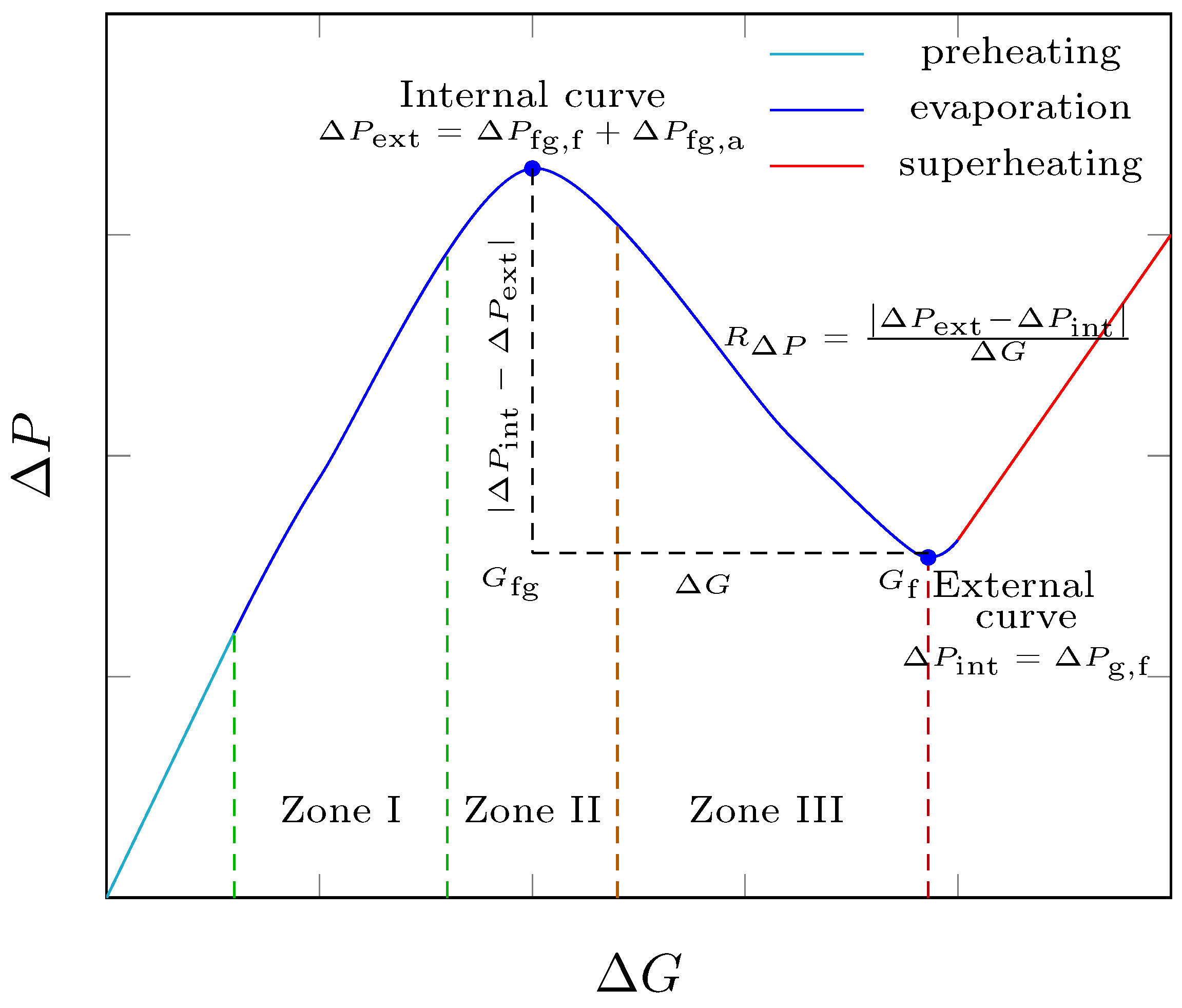
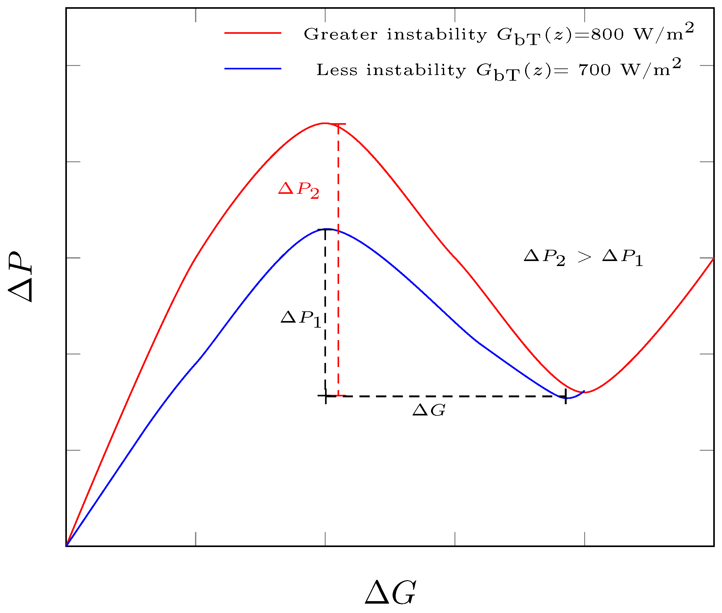
Figure 4 shows the behavior of the pressure drop with respect to the mass flow of water in the evaporation region of the concentrator loop. In this region, the pressure drop of the liquid–vapor mixture along the loop, $\Delta P_{\mathrm{fg}}$, as expressed by Equation (27), has a component associated with the acceleration of the vapor phase, $\Delta P_{\mathrm{fg},\mathrm{a}}$, as expressed by Equation (28), and another related to the friction of the liquid with the wall, $\Delta P_{\mathrm{fg},\mathrm{f}}$, as expressed by Equation (30). This behavior indicates the presence of flow instability, also known as evaporation velocity, which is visualized in Figure 4 as an oscillation of pressure drops, whose characteristic curve is “N”-shaped and is the union of the internal curves (blue curve—concave downward) and external curves (red curve—concave upward).

Throughout the oscillation, the components of the pressure drop in the evaporation region were competing with each other, thus causing a change in the concavity of the oscillation. This allowed us to identify the following areas of instability evolution:

• Zone I: The fall of $R_{\Delta P}$ because the acceleration of the vapor phase dominates, i.e., $\Delta P_{\mathrm{fg},\mathrm{a}}\gg \Delta P_{\mathrm{fg},\mathrm{f}}$. This area corresponds to the expanding portion of the internal curve.
• Zone II: The pressure drops because the acceleration of the vapor phase and the friction of the liquid with the wall have the same order of magnitude, i.e., $\Delta P_{\mathrm{fg},\mathrm{a}}\approx \Delta P_{\mathrm{fg},\mathrm{f}}$. This zone corresponds to the set of points of the oscillation traversing from the crest (maximum internal curve) to the trough of the oscillation and contains the inflection point of the oscillation.
• Zone III: Pressure drops due to the friction of the liquid with the wall are dominant, i.e., $\Delta P_{\mathrm{fg},\mathrm{a}}\ll \Delta P_{\mathrm{fg},\mathrm{f}}$. This area coincides with the expanding region of the external curve.

The magnitude of flow instability is estimated using the slope, $R_{\Delta P}$ in m/s, of the straight line that passes through the crest (maximum of the internal curve) and valley (minimum of the external curve) of the oscillation [36]:

$$R_{\Delta p}={\displaystyle \frac{\left|\Delta P_{\mathrm{ext}}-\Delta P_{\mathrm{int}}\right|}{\Delta G}}$$

(31)

Figure 5 shows the influence of the incidence of effective solar irradiance that affects the receiver and that is transferred to the mass flow of water that circulates along the loop on the magnitude of the instability. The greater the solar irradiance absorbed by the receiver and supplied to the working fluid, the greater the instability magnitude. Consequently, the pressure drops because the acceleration of the steam and the friction between the wall and water have the same order of magnitude.

4.3. Liquid Elevation Angle in Stratified Flow Pattern

In the $xy$ plane, the liquid elevation angle, $\theta$, is the angle formed by the y axis and the radius of the internal wall of the receiving tube that intersects the liquid surface of the stratified liquid–vapor flow, as shown in Figure 6. This angle varies as the liquid water evaporates along the receiving tube and is thus a function of the liquid–vapor mixture quality. The angle of elevation of the liquid is useful for determining the surfaces of the inner wall of the tube that are in contact with the liquid and vapor phases. Therefore, it facilitates the establishment of boundary conditions at the fluid–internal wall interface of the tube.

In this study, the liquid elevation angle for a liquid–vapor mixture that reflects a stratified flow pattern, based on [37], is expressed as the liquid surface area in terms of the product of the cross-sectional area of the receiving tube and the mass fraction of liquid in the liquid–vapor mixture. Additionally, it can be expressed as a function of the radius and internal angle of the wall of the receiving tube, $R_{\mathrm{i}}$ and ${\theta }_{\mathsf{\ell }}$.

$$\begin{array}{c}\hfill {\theta }_{\mathsf{\ell }}=sin{\theta }_{\mathsf{\ell }}cos{\theta }_{\mathsf{\ell }}+{\displaystyle \frac{(1-x){\dot{m}}_{\mathrm{loop}}}{{\rho }_{\mathrm{f}}{u}_{\mathrm{f}}{R}_{\mathrm{i}}^2}}\end{array}$$

(32)

The numerical solution to the previous equation is obtained using the Newton–Raphson method. Using linear regression, the following correlation was obtained for ${\theta }_{\mathsf{\ell }}$ as a function of quality for different compositions in the composite wall of the receiving tube, based on a correlation coefficient of 0.9994 and values $A_{\mathrm{t}}$ = 0.00332 m², $R_{\mathrm{i}}$ = 0.035 m, and ${\dot{m}}_{\mathrm{loop}}$ = 0.72 kg/s.

$${\theta }_{\mathsf{\ell }}=-180x+90$$

(33)

Once the internal angle of the receiving tube wall is defined, the velocities of each phase are expressed as follows:

$$\begin{array}{ccc}\hfill u_{\mathrm{f}}={\displaystyle \frac{(1-x){\dot{m}}_{\mathrm{loop}}}{{\rho }_{\mathrm{f}}\left(\pi R_{\mathrm{i}}^2-\frac{x{\dot{m}}_{\mathrm{loop}}}{u_{\mathrm{g}}{\rho }_{\mathrm{g}}}\right)}}& \hfill & \hfill u_{\mathrm{g}}={\displaystyle \frac{x{\dot{m}}_{\mathrm{loop}}}{{\rho }_{\mathrm{g}}{A}_t\epsilon }}\end{array}$$

(34)

5. Heat Transfer in Copper–Alumina Composite Wall of Receiving Tube

To determine the heat transport in the composite wall of the receiving tube, the study is separated into cases for alumina ($\alpha$) and copper ($\kappa$) based on the schemes shown in Figure 2 and Figure 6. The equations that model the transport and angle $\theta$-dependent outer boundary conditions for the $\alpha$-region over the total length of the loop or $z\in (0,L_{\mathrm{loop}})$ are as follows:

$$\begin{array}{c}{\displaystyle \frac{1}{{\alpha }_{\alpha }}}{\displaystyle \frac{\partial T_{\alpha }}{\partial t}}={\displaystyle \frac{1}{r}}{\displaystyle \frac{\partial }{\partial r}}\left({\displaystyle \frac{\partial T_{\alpha }}{\partial r}}\right)+{\displaystyle \frac{1}{r^2}}{\displaystyle \frac{\partial }{\partial \theta }}\left({\displaystyle \frac{\partial T_{\alpha }}{\partial \theta }}\right)+{\displaystyle \frac{\partial }{\partial z}}\left({\displaystyle \frac{\partial T_{\alpha }}{\partial z}}\right)\end{array}$$

(35a)

$$\begin{array}{c}\mathrm{en}t=0T_{\alpha }={\displaystyle \frac{T_1+T_{10}}{2}}\end{array}$$

(35b)

$$\begin{array}{c}-k_{\alpha }{\displaystyle \frac{\partial T_{\alpha }}{\partial r}}=G_{bT}\left(z\right),r=R_{\mathrm{o}},\theta \in (0,\pi )\end{array}$$

(35c)

$$\begin{array}{c}-k_{\alpha }{\displaystyle \frac{\partial T_{\alpha }}{\partial r}}=R_c{G}_{bT}\left(z\right),r=R_{\mathrm{o}},\theta \in (\pi ,2\pi )\end{array}$$

(35d)

$$\begin{array}{c}-k_{\alpha }{\displaystyle \frac{\partial T_{\alpha }}{\partial z}}=0,z=0,L_{\mathrm{loop}},\end{array}$$

(35e)

where $G_{\mathrm{bT}}\left(z\right)$ denotes the solar irradiance expressed in Equation (7) and $R_c$ is the ratio of the collection area of the receiving tube to that of the concentrator parabola, as expressed in Equation (1). The boundary conditions at the entrance and exit of the system are specified as thermal insulation. For the boundary condition between alumina and copper, heat continuity is considered because heat dissipation occurs through direct contact. Although both the materials are good conductors, some resistance to heat transfer through the interface occurs because of imperfections, surface roughness, and microscopic air spaces [38].

This resistance is typically quantified as the thermal contact resistance. Additionally, copper and alumina have different coefficients of thermal expansion, which can cause dimensional changes when heated or cooled. This difference in thermal expansion can cause stress at the interface, which can result in mechanical problems if not considered in the design [39]. In this case, the contributions of stress at the interface, as well as those of radiation and convection owing to their thickness, are disregarded. This is based on Fourier’s law of heat conduction, in which the rate of heat transfer per unit area is proportional to the temperature gradient across two different materials [40,41]. In the case of copper and alumina, the heat flow across the interface is continuous, which ensures a constant heat transfer. Therefore, the average characteristics of copper and alumina were considered in the design systems for effective heat transfer. Meanwhile, the thermal properties at the Cu–Al₂O₃ interface (or $\kappa$–$\alpha$ interface) were estimated from the arithmetic average of the property of each corrected material.

$${\psi }_{\kappa \text{–}\alpha }={\displaystyle \frac{{\psi }_{\kappa }+{\psi }_{\alpha }}{2}}+{\displaystyle \frac{w_{\kappa }{\psi }_{\kappa }{w}_{\alpha }{\psi }_{\alpha }}{w_{\kappa }{\psi }_{\kappa }+w_{\alpha }{\psi }_{\alpha }}},$$

(36)

where $\psi$ assumes the values of the thermal properties k, $C_P$, and $\rho$ in each case and $w_{\kappa }$ and $w_{\alpha }$ are the material fractions of copper and alumina, respectively. For copper ($\kappa$region), three flow regions that occur during steam generation were established: preheating $\left(0\le z\le L_{\mathrm{f}}\right)$, evaporation $\left(L_{\mathrm{f}}<z\le L_{\mathrm{fg}}\right)$, and superheating $\left(L_{\mathrm{fg}}<z\le L_{\mathrm{loop}}\right)$. Subsequently, a differential equation and boundary conditions were established by considering thermal insulation at the entrance and exit of the system.

$$\begin{array}{c}{\displaystyle \frac{1}{{\alpha }_{\kappa }}}{\displaystyle \frac{\partial T_{\kappa }}{\partial t}}={\displaystyle \frac{1}{r}}{\displaystyle \frac{\partial }{\partial r}}\left({\displaystyle \frac{\partial T_{\kappa }}{\partial r}}\right)+{\displaystyle \frac{1}{r^2}}{\displaystyle \frac{\partial }{\partial \theta }}\left({\displaystyle \frac{\partial T_{\kappa }}{\partial \theta }}\right)+{\displaystyle \frac{\partial }{\partial z}}\left({\displaystyle \frac{\partial T_{\kappa }}{\partial z}}\right)\end{array}$$

(37a)

$$\begin{array}{c}\mathrm{en}t=0T_{\kappa }={\displaystyle \frac{T_1+T_{10}}{2}}\end{array}$$

(37b)

$$\begin{array}{c}\mathrm{preheating}:-k_{\kappa }{\displaystyle \frac{\partial T_{\kappa }}{\partial r}}=h_{\mathrm{cf}}\left(T_{\mathrm{f}}-T_{\kappa }\right),\theta \in (0,2\pi )\end{array}$$

(37c)

$$\begin{array}{c}\mathrm{evaporation}:-k_{\kappa }{\displaystyle \frac{\partial T_{\kappa }}{\partial r}}=h_{\mathrm{cf}}\left(T_{\mathrm{sat}}-T_{\kappa }\right),\theta \in (0,{\theta }_{\mathsf{\ell }})\end{array}$$

(37d)

$$\begin{array}{c}\mathrm{evaporation}:-k_{\kappa }{\displaystyle \frac{\partial T_{\kappa }}{\partial r}}=h_{\mathrm{cg}}\left(T_{\mathrm{sat}}-T_{\kappa }\right),\theta \in ({\theta }_{\mathsf{\ell }},2\pi )\end{array}$$

(37e)

$$\begin{array}{c}\mathrm{superheating}:-k_{\kappa }{\displaystyle \frac{\partial T_{\kappa }}{\partial r}}=h_{\mathrm{cg}}\left(T_{\mathrm{g}}-T_{\kappa }\right),\theta \in (0,2\pi )\end{array}$$

(37f)

$$\begin{array}{c}-k_{\kappa }{\displaystyle \frac{\partial T_{\kappa }}{\partial z}}=0,z=0,L_{\mathrm{loop}},\end{array}$$

(37g)

where $h_{\mathrm{cf}}$ and $h_{\mathrm{cg}}$ are the convective heat transfer coefficients for the liquid water and vapor phases, respectively, as expressed in Equation (23), and $T_{\mathrm{f}}$, $T_{\mathrm{sat}}$, and $T_{\mathrm{g}}$ are the water temperatures in the preheating, evaporation, and superheating regions, respectively, which are obtained from Equations (20) and (24). In Equations (37d) and (37e), ${\theta }_{\mathsf{\ell }}$ is the elevation angle of the liquid in the evaporation region and is determined from Equations (32) and (33).

For a detailed description of the numerical methodology used for the heat transfer analysis in the composite wall of the receiver, please refer to Appendix B, where the procedure is outlined using COMSOL Multiphysics software.

6. Results

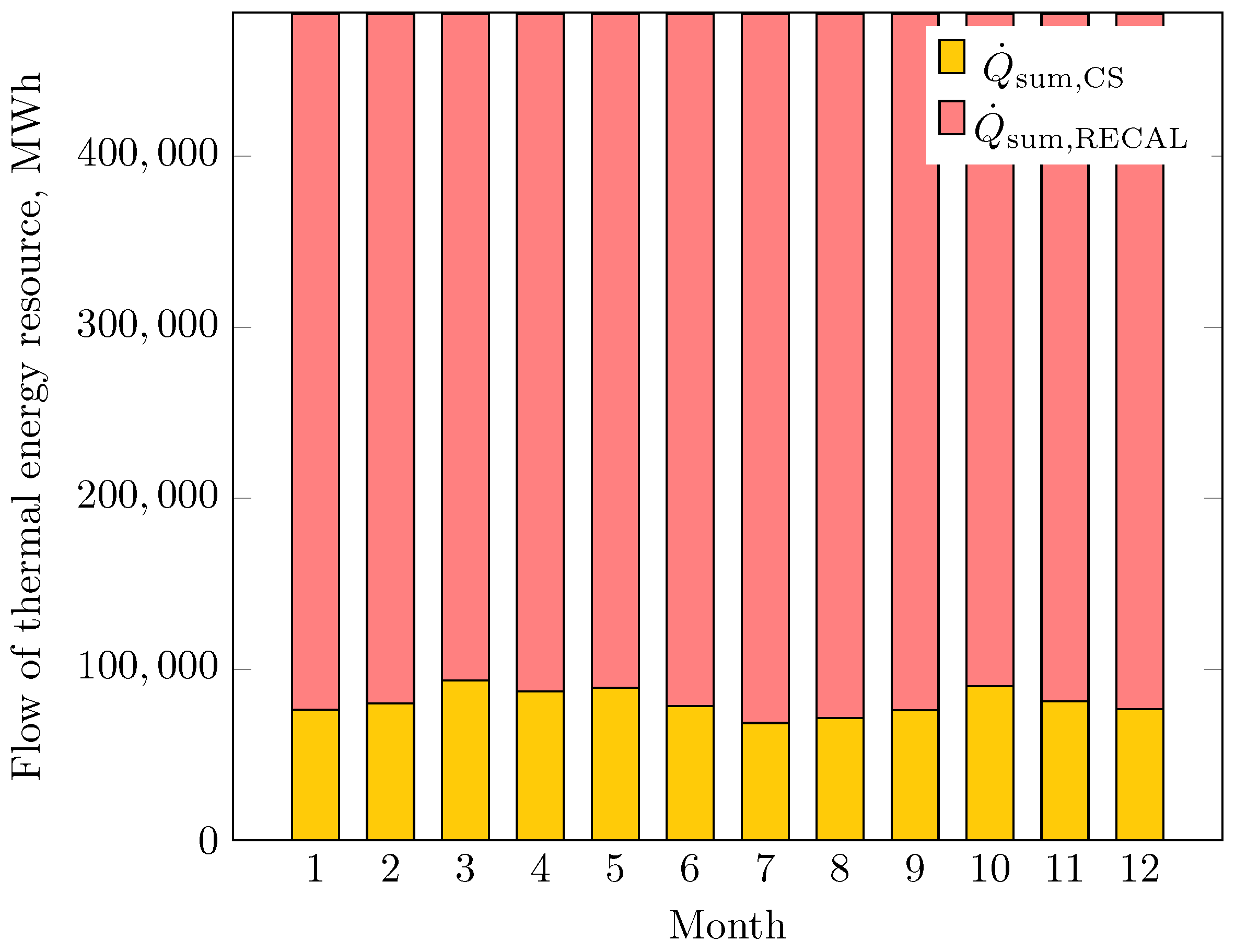
The heat flow requirements that the SF and RH must provide to supply 483,228.00 MWh/month to the power cycle for the plant to generate 50 MW_e and operate at 100% throughout the year are shown in Figure 7. The heat flow contributed by the SF was between 14% and 19% of the total thermal energy requirement. This contribution reaches its minimum during winter and its maximum at the beginning of spring. Because of this solar intermittency, the ASG supplies between 81% and 86% of the thermal energy to the power cycle. Based on these results, the sizing of the SF of the hybrid solar plant was performed.

During the spring solstice, the solar thermal plant generates 50 MW_e and is supplied with ${\dot{Q}}_{\mathrm{sum},\mathrm{SF}}$ = 113.21 MW_th and ${\dot{Q}}_{\mathrm{sum},\mathrm{RH}}$ = 113.21 MW_th to achieve a water flow of ${\dot{m}}_T$ = 53.01 kg/s with a thermal efficiency of ${\eta }_{th}$ = 0.41. Under the design conditions established in Section 3 and the equations presented in Section 3.3, the powers generated by the HPT and LPT as well as the power requirements of the HPP and LPP are presented in

Table 1. Energy requirements of components of hybrid solar–thermal plant.

Components	$\dot{\mathit{W}}$, MW	Energy Balance
HPT	16.13	${\dot{m}}_1\left(h_1-h_2\right)$
LPT	39.35	${\dot{m}}_3\left(h_3-h_7\right)+{\dot{m}}_4\left(h_7-h_4\right)$
HPP	0.76	${\dot{m}}_T\left(h_9-h_8\right)$
LPP	0.013	${\dot{m}}_4\left(h_6-h_5\right)$
Component	$\dot{\mathbf{Q}}\mathbf{,}{\mathbf{MW}}_{\mathbf{th}}$	Energy Balance
SF	113.21	${\dot{m}}_T\left(h_1-h_{10}\right)$
RH	21.08	${\dot{m}}_3\left(h_3-h_2\right)$
COND	84.29	${\dot{m}}_4\left(h_4-h_5\right)$

.

For the sizing of the SF, it is assumed that the receiving tube comprises a borosilicate glass cover and a wall composed of 50% copper UNS 12200 Cu and 50% alumina Al₂O₃, whose thickness is $R_{\mathrm{o}}-R_{\mathrm{i}}>0$ with $R_{\mathrm{o}}$ = 0.035 m and $R_{\mathrm{i}}$ = 0.030 m. The thickness of the Cu and Al₂O₃ walls is 0.0025 m.

Table 2. Solar field design features for 925 m-long loops.

Quantity	Concentrator	Loop	Field
${\dot{Q}}_{\mathrm{u}},\mathrm{kW}$	257.42	$1544.52$	134,230
$\dot{m},\mathrm{kg}/\mathrm{s}$	0.67	0.72	53.01
$N_{\mathrm{conc}}$	1	6	522

lists the design characteristics of the SF obtained from the assumptions established in Section 3 and the application of the sizing equations. The U-shaped SF comprises 87 loops composed of six concentrators with length $L_{\mathrm{loop}}=925$ m connected in series.

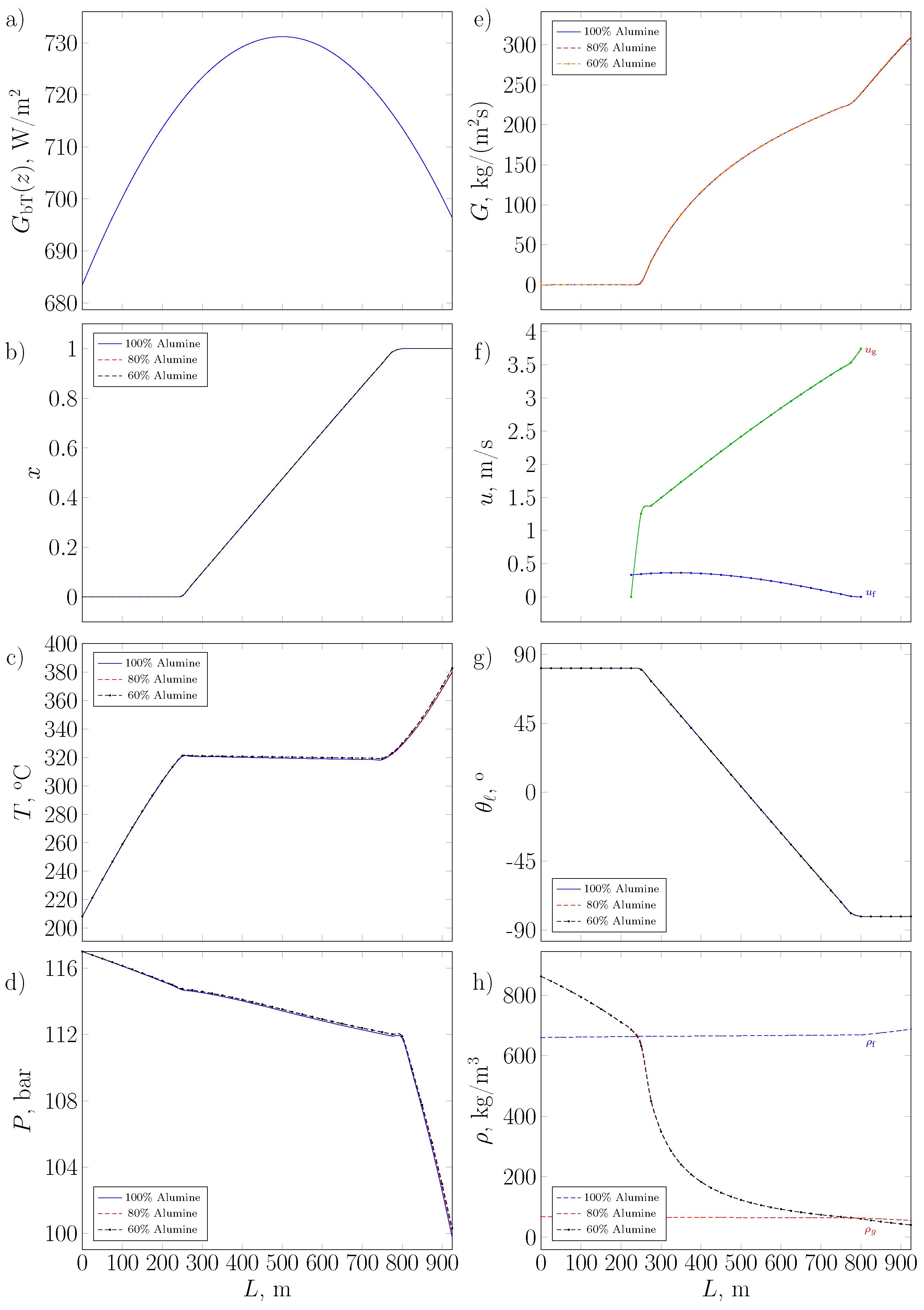
Figure 8a shows the profile of the direct irradiance incident on the receiving tube in the axial direction during the spring solstice. This profile was used to estimate the thermodynamic and transport properties of water along the concentrator loop and the elevation angle of the liquid in the evaporation region for different Cu-Al₂O₃ ratios in the composite walls of the receiver tubes.

Figure 8b shows the vapor quality profile along the evaporation region of a concentrator loop for Al₂O₃ ratios of 60%, 80%, and 100%, This figure indicates that preheating occurred in the first 250 m, the evaporation region with $x\in 0,0.88$ began at 250 m and ended between 789.73 and 797.28 m of the loop, and overheating occurred between the final 141.25 and 127.72 m. The length of the evaporation region increased with the percentage of alumina in the receiver wall because the thermal conductivity of alumina is ten times lower than that of copper.

Figure 8c shows that, in the preheating region, the water temperature increased from 208.2 °C to approximately 321.05 °C for the different compositions on the wall of the receiving tube. In the evaporation region, the water temperature remained at approximately 320.02 °C. Finally, in the superheating region, the water temperature increased from approximately 320.08 °C to approximately 383.04 °C.

Figure 8d shows the pressure profiles along the concentrator loop. In the preheating region, the water pressure at the receiving tube wall decreased from 117 bar to approximately 114.77 bar for different compositions. In the evaporation region, the water pressure decreased from approximately 114.77 bar to 111.92 bar. Finally, in the superheating region, the pressure decreased from 111.92 bar to approximately 100.44 bar. At first glance, this figure presents a continuous pressure drop along the loop; however, in the transition between the evaporation and superheating regions, an increase in water pressure of 0.12 bar occurred between 760 and 795 m.

Figure 8e shows the increase in mass flow of the vapor phase along the concentrator loop in the evaporation and superheating regions. The mass flow growth rate in the evaporation region was lower than that in the superheating region because of the increase in the vapor fraction in this zone. The decrease in the slope of the mass flow between 760 and 795 m, as shown in Figure 8d, increased the pressure drop, which increased the magnitude of the flow instability in the transition region between evaporation and overheating.

Figure 8f shows the behavior of the fluid and vapor velocities. The fluid velocity remained constant at 0.25 m/s along the loop until the phase changed to vapor, at which it decayed to 0. Meanwhile, the vapor velocity increased from 0 to 1.5 m/s in the loop up to 250 m. Subsequently, it increased linearly up to 760 m and then increased in the final section of the loop, which was in accordance with the changes in the pressure drop.

Figure 8g shows that the elevation angle of the liquid in the preheating region was 0.88, whereas the elevation angle with respect to the axial direction decreased linearly in the evaporation region.

Figure 8h shows the density of the working fluid as it traversed through the concentrator loop. In the preheating region, the density of liquid water decreased from 862.63 kg/m³ to approximately 686.23 kg/m³ for the different receiver tube compositions. In the evaporation region, the density of the mixture decreased gradually until it reached approximately 686.25 kg/m³. In the superheating region, the density of the mixture decreased to 40.997 kg/m³ for the different compositions. Changes in the density increased the magnitude of flow instability, which was primarily owing to the increase in pressure drop since the changes in the mass flow were less significant [42].

To determine the effect of the Cu-Al₂O₃ ratio of the composite wall of the receiving tubes on the DSG in the evaporation region, the effect of the composition of the composite wall of the receiving tubes on the length is presented in Figure 9. Additionally, the effects of the composition of the composite wall of the receiving tubes on the length, pressure drop, and magnitude of flow instability in the evaporation region is presented. This figure shows that an increase in the proportion of alumina in the composite wall of the receiving tube increased the magnitude of the evaporation region, pressure drop, and maximum temperature difference on the wall of the receiver, whereas it decreased the magnitude of flow instability owing to the increase in thermal conductivity. In addition, it decreased the steam temperature at the outlet of the concentrator loop.

In this study, a 50% Cu–50% Al₂O₃ proportion was considered for the sizing of the SF to manage the magnitudes of flow instability and maximum intermediate tube wall temperature differences that favor the mechanical integrity and thermal properties of the concentrator loop. Notably, the proportion is available commercially. Under this proportion, the saturation condition was attained 3.14 m earlier than in the case of the 100% alumina wall. When comparing the effect of 50% and 100% Al₂O₃ on the walls of the receiving tube, the pressure drop reduced by 3.3%, the magnitude of flow instability increased by 5.03%, and the difference in the maximum temperatures was 48.37 °C. Considering the result based on 40% Cu–60% Al₂O₃ and comparing it with that of the 100% Al₂O₃ wall, the instability magnitude increased by 3.06%, the saturation condition was attained 3.02 m before the wall with 100% Al₂O₃, and the pressure drop reduced by 3.1%, and the reduction in the maximum temperature difference was 44.23 °C.

The composite wall was evaluated ($\Delta T_{\max }$) at times $t=3,6,9,12$, and 15 min, as shown in Figure 10.

Figure 11 shows the behavior of the temperatures in the cross-section of the wall composed of 40% Cu and 60% Al₂O₃ of the receiving tube for z = 629 m at times t = 3, 6, 9, 12, and 15 min during the spring solstice.

The highest temperature of the wall of the receiving tube with a proportion of 40% Cu–60% Al₂O₃ was analyzed in the hot spot formation zone for t = 15 min.

Figure 12 shows that the highest temperature of the tube was 618.11 K, which was located on the external wall ($r=R_{\mathrm{o}}$) at $\theta \in$ 198°, 217°, i.e., the location where the concentrated direct solar irradiance exerted its effects.

7. Conclusions

The dynamics of the numerical solution of the model was analyzed in the cross-sections of the composite wall. In this regard, a value for z was set, and the effects of r and $\theta$ on the maximum temperature difference in the composite wall were evaluated ($\Delta T_{\max }$).

In the preheating region, $\Delta T_{\max }$ increased with the length of the concentrator loop by approximately 0.656 °C/m and 0.354 °C/m for 10% and 50% alumina, respectively. In this region, the numerical solutions for different proportions of alumina reached the steady state rapidly because, when comparing a solution at time $t_{i+1}$ with that at time $t_i$, the difference increased from 0.03 to 1.47 $\times {10}^{-2}$ °C. This indicates that, at any instant, the wall temperature was almost uniform.

In addition, in the evaporation region, $\Delta T_{\max }$ presented between five and six changes in the concavity with respect to the length of the concentrator loop. These concavities were different from those of $\Delta P$ as a function of z. These behaviors suggested coupled mechanical and thermal instabilities.

Thermal behavior at the tube wall showed abrupt changes in the $\Delta T_{\max }$, e.g., for the 50% alumina, $\Delta T_{\max }$ increased from 9.1 °C at the beginning of the evaporation region (z = 250 m and $x=0$) to 4.6 °C for $z=517.1$ m ($x=0.522$) and subsequently reached a global maximum at 25.2 °C for $z=729.3$ m ($x=0.9$).

The evaporation region zone that included the maximum value of $\Delta T_{\max }$ was between 744.6 and 760.1 m for 50% and 10% alumina proportions. In this area, hot spots appeared on the tube wall, accompanied by pressure increases from 0.128 to 1.94 bar.

These numerical results are consistent with the experimental evidence of the receptor softening and deformation [43,44]. In addition, in the superheating region, $\Delta T_{\max }$ did not exceed 0.5 °C, thus indicating that the temperature on the tube wall was uniform.

In the receiving tube for z = 629 m at times t = 3, 6, 9, 12, and 15 min, hot spots appeared between 517.1 m ($x=0.522$) and 729.3 m ($x=0.9$) in the evaporation region at $t>0$; meanwhile, in the preheating and superheating regions, the wall temperature was almost uniform.

The highest temperature of the tube was 618.11 K, which was located on the external wall ($r=R_{\mathrm{o}}$) at $\theta \in$ 198°, 217°, i.e., the location where the concentrated direct solar irradiance exerted its effects. Meanwhile, the lowest temperature of 602.13 K was indicated at $\theta$ = 90°, where direct solar irradiation exerted its effects.

The maximum differences in each solid phase of the composite wall of the receiving tube were 10.86 °C and 4.37 °C, and the minimum differences were 0.25 °C and 0.04 °C for alumina and copper, respectively. Owing to its thermal properties, copper favored the transfer of heat to the working fluid, whereas alumina, which is a ceramic material, served as a thermal deposit that suppressed the softening effects in the solid phase of copper. These results indicate that the alumina wall reduced the effects of thermal instability that would occur in an alumina-free copper tube, which would result in the deformation of the tube with the effects of flow instabilities.

8. Summary of Results

The following tables (

Table 3. Plant performance and configuration.

Parameter	Value	Notes
Total power generation	50 MWe	Operating at 100% throughout the year
Solar field contribution	14–19%	Minimum in winter, maximum in early spring
ASG contribution	81–86%	Compensates for solar intermittency
Thermal efficiency (${\eta }_{\mathrm{th}}$)	0.41	Under design conditions

,

Table 4. Solar field design characteristics.

Component	Specifications	Details
Loop configuration	U-shaped	87 loops total
Loop length	925 m	6 concentrators per loop
Total concentrators	522	Across entire field
Mass flow rate	53.01 kg/s	Total field flow rate
Useful heat (${\dot{Q}}_{\mathrm{u}}$)	134,230 kW	Total thermal power

,

Table 5. Receiving tube characteristics.

Parameter	Value/Range	Notes
Wall composition	50% Cu–50% Al2O3	Optimized ratio
Tube dimensions	$R_{\mathrm{o}}$ = 0.035 m, $R_{\mathrm{i}}$ = 0.030 m	Outer and inner radius
Wall thickness	0.0025 m	For each material

,

Table 6. Temperature and pressure profiles.

Region	Temperature Range	Pressure Range
Preheating	208.2 °C–321.05 °C	117–114.77 bar
Evaporation	∼320.02 °C (constant)	114.77–111.92 bar
Superheating	320.08 °C–383.04 °C	111.92–100.44 bar

,

Table 7. Critical findings for 40% Cu–60% Al₂O₃ wall.

Parameter	Value	Location/Condition
Highest tube temperature	618.11 K	At $\theta \in$ 198°–217°
Lowest tube temperature	602.13 K	At $\theta$ = 90°
Maximum temperature difference (Al2O3)	10.86 °C	In ceramic phase
Maximum temperature difference (Cu)	4.37 °C	In metallic phase
Minimum temperature difference (Al2O3)	0.25 °C	In ceramic phase
Minimum temperature difference (Cu)	0.04 °C	In metallic phase

and

Table 8. Performance comparisons (vs. 100% Al₂O₃).

Parameter	50% Cu–50% Al2O3	40% Cu–60% Al2O3
Saturation point difference	3.14 m earlier	3.02 m earlier
Pressure drop reduction	3.3%	3.1%
Flow instability increase	5.03%	3.06%
Maximum temperature difference	48.37 °C lower	44.23 °C lower

) highlight the most important numerical results and their relationships, making it easier to understand the key outcomes of the study.

References

1. Visconti, P.; Ria, R.; Cavalera, G. Development of smart PIC–based electronic equipment for managing and monitoring energy production of photovoltaic plan with wireless transmission unit. J. Eng. Appl. Sci. 2015, 10, 9434–9441. [Google Scholar]
2. Wright, S.A.; Pickard, P.S.; Fuller, R.; Radel, R.F.; Vernon, M.E. Supercritical CO2 Brayton cycle power generation development program and initial test results. In Proceedings of the ASME Power Conference, Albuquerque, NM, USA, 21–23 July 2009; pp. 573–583. [Google Scholar]
3. Stutz, B.; Le Pierres, N.; Kuznik, F.; Johannes, K.; Del Barrio, E.P.; Bedecarrats, J.P.; Gibout, S.; Marty, P.; Zalewski, L.; Soto, J. Storage of thermal solar energy. Comptes Rendus Phys. 2017, 18, 401–414. [Google Scholar] [CrossRef]
4. Visconti, P.; Primiceri, P.; Costantini, P.; Colangelo, G.; Cavalera, G. Measurement and control system for thermosolar plant and performance comparison between traditional and nanofluid solar thermal collectors. Int. J. Smart Sens. Intell. Syst. 2016, 9, 1220–1242. [Google Scholar] [CrossRef]
5. Eck, M.; Steinmann, W.D. Direct steam generation in parabolic troughs: First results of the DISS project. J. Sol. Energy Eng. 2002, 124, 134–139. [Google Scholar] [CrossRef]
6. Price, H.; Lüpfert, E.; Kearney, D.; Zarza, E.; Cohen, G.; Gee, R.; Mahoney, R. Advances in parabolic trough solar power technology. J. Sol. Energy Eng. 2002, 124, 109–125. [Google Scholar] [CrossRef]
7. Zarza, E.; Valenzuela, L.; León, J.; Weyers, H.D.; Eickhoff, M.; Eck, M.; Hennecke, K. The DISS project: Direct steam generation in parabolic trough systems. Operation and maintenance experience and update on project status. J. Sol. Energy Eng. 2002, 124, 126–133. [Google Scholar] [CrossRef]
8. Zarza, E.; Valenzuela, L.; Leon, J.; Hennecke, K.; Eck, M.; Weyers, H.D.; Eickhoff, M. Direct steam generation in parabolic troughs: Final results and conclusions of the DISS project. Energy 2004, 29, 635–644. [Google Scholar] [CrossRef]
9. Aritomi, M.; Aoki, S.; Inoue, A. Instabilities in parallel channel of forced-convection boiling upflow system, (I) Mathematical model. J. Nucl. Sci. Technol. 1977, 14, 22–30. [Google Scholar] [CrossRef]
10. Davies, A.; Potter, R. Hydraulic Stability: An Analysis of the Causes of Unstable Flow in Parallel Channels; UKAEA, Winfrith, Atomic Energy Establishment: Abingdon, UK, 1966. [Google Scholar]
11. Kakaç, S.; Ozboya, N. Transient boiling flow instabilities in a multi-channel upflow-system. Waerme-Stoffuebertrag 1977, 10, 175–188. [Google Scholar] [CrossRef]
12. Boiling Flow Instabilities in Parallel Channels; SAGE Publications: London, UK, 1969; Volume 184.
13. Wang, B.; Hu, Y.; He, Y.; Rodionov, N.; Zhu, J. Dynamic instabilities of flow boiling in micro-channels: A review. Appl. Therm. Eng. 2022, 214, 118773. [Google Scholar] [CrossRef]
14. Xiao, M.; Chen, X.; Zhang, M.; Veziroglu, T.; Kakac, S. A multivariable linear investigation of two-phase flow instabilities in parallel boiling channels under high pressure. Int. J. Multiph. Flow 1993, 19, 65–77. [Google Scholar] [CrossRef]
15. Ozawa, M. Flow instability problems in steam-generating tubes. In Steam Power Engineering-Thermal and Hydraulic Design Principles; Cambridge University Press: Cambridge, UK, 1999; pp. 323–385. [Google Scholar]
16. Tafuni, A.; Giannotta, A.; Mersch, M.; Pantaleo, A.; Amirante, R.; Markides, C.; De Palma, P. Thermo-economic analysis of a low-cost greenhouse thermal solar plant with seasonal energy storage. Energy Convers. Manag. 2023, 288, 117–123. [Google Scholar] [CrossRef]
17. Mundo-Hernández, J.; de Celis Alonso, B.; Hernández-Álvarez, J.; de Celis-Carrillo, B. An overview of solar photovoltaic energy in Mexico and Germany. Renew. Sustain. Energy Rev. 2014, 31, 639–649. [Google Scholar] [CrossRef]
18. Aqachmar, Z.; Allouhi, A.; Jamil, A.; Gagouch, B.; Kousksou, T. Parabolic trough solar thermal power plant Noor 1 in Morocco. Energy 2019, 178, 572–584. [Google Scholar] [CrossRef]
19. Salazar, G.A.; Fraidenraich, N.; de Oliveira, C.A.A.; de Castro Vilela, O.; Hongn, M.; Gordon, J.M. Analytic modeling of parabolic trough solar thermal power plants. Energy 2017, 138, 1148–1156. [Google Scholar] [CrossRef]
20. Silva, R.; Pérez, M.; Fernández-Garcia, A. Modeling and co-simulation of a parabolic trough solar plant for industrial process heat. Appl. Energy 2013, 106, 287–300. [Google Scholar] [CrossRef]
21. Duffie, J.A.; Beckman, W.A. Solar Engineering of Thermal Processes; John Wiley & Sons: Hoboken, NJ, USA, 2013. [Google Scholar]
22. Benato, A.; Kærn, M.R.; Pierobon, L.; Stoppato, A.; Haglind, F. Analysis of hot spots in boilers of organic Rankine cycle units during transient operation. Appl. Energy 2015, 151, 119–131. [Google Scholar] [CrossRef]
23. Dickes, R.; Dumont, O.; Guillaume, L.; Quoilin, S.; Lemort, V. Charge-sensitive modelling of organic Rankine cycle power systems for off-design performance simulation. Appl. Energy 2018, 212, 1262–1281. [Google Scholar] [CrossRef]
24. Helvaci, H.; Khan, Z. Thermodynamic modelling and analysis of a solar organic Rankine cycle employing thermofluids. Energy Convers. Manag. 2017, 138, 493–510. [Google Scholar] [CrossRef]
25. Shoeibi, S.; Kargarsharifabad, H.; Sadi, M.; Arabkoohsar, A.; Mirjalily, S.A.A. A review on using thermoelectric cooling, heating, and electricity generators in solar energy applications. Sustain. Energy Technol. Assess. 2022, 52, 102–105. [Google Scholar] [CrossRef]
26. Islam, S.; Dincer, I.; Yilbas, B.S. Development, analysis and assessment of solar energy-based multigeneration system with thermoelectric generator. Energy Convers. Manag. 2018, 156, 746–756. [Google Scholar] [CrossRef]
27. Psiloglou, B.; Kambezidis, H.; Kaskaoutis, D.; Karagiannis, D.; Polo, J. Comparison between MRM simulations, CAMS and PVGIS databases with measured solar radiation components at the Methoni station, Greece. Renew. Energy 2020, 146, 1372–1391. [Google Scholar] [CrossRef]
28. Wang, Z. Design of Solar Thermal Power Plants; Academic Press: Cambridge, MA, USA, 2019. [Google Scholar]
29. Torres-Aldaco; Romero Paredes, H.; Ambriz, J.J. Modelamiento de un lecho fluidizado a altas temperaturas. In Proceedings of the XXI Semana Nacional de Energía Solar, Chihuahua, Mexico, 1–3 October 1997; Asociación Nacional 679 de Energía Solar, AC (ANES): Ciudad de México, Mexico, 1997; Volume 10, pp. 334–338. [Google Scholar]
30. Acuna, A.; Velázquez, N.; Sauceda, D.; Aguilar, A. Modeling, construction, and experimentation of a compound parabolic concentrator with a concentric tube as the absorber. J. Energy Eng. 2017, 143, 0733–9402. [Google Scholar] [CrossRef]
31. Sharma, M.P.; Tiselj, I.; Kren, J.; Mikuž, B.; Cizelj, L. Thermal streak spacing in fully developed duct flow with different Reynolds and Prandtl numbers. Heat Mass Transf. 2023, 59, 2105–2116. [Google Scholar] [CrossRef]
32. Lu, Y.; Deng, S.; Nie, X.; Zhao, L.; Wang, D.; Zhao, D.; Chen, L. Ledinegg instability analysis on direct vapor generation inside solar collectors. Sol. Energy 2020, 196, 530–539. [Google Scholar] [CrossRef]
33. Ruvo, T.H.; Saha, S.; Mojumder, S.; Saha, S. Mixed convection in an open T-shaped cavity utilizing the effect of different inflow conditions with Al2O3-water nanofluid flow. Results Eng. 2023, 17, 100862. [Google Scholar] [CrossRef]
34. Daneshvar, F.A.; Talebbeydokhti, N.; Dehghan, S.M.; Elhamian, S.M.M. Evaluation of Darcy–Weisbach Friction Factors of Fiberglass Pipes Based on Internal Surface Roughness Measurement. Iran. J. Sci. Technol. Trans. Civ. Eng. 2023, 47, 1749–1762. [Google Scholar] [CrossRef]
35. Zeguai, S.; Chikh, S.; Tadrist, L. Experimental study of two-phase flow pattern evolution in a horizontal circular tube of small diameter in laminar flow conditions. Int. J. Multiph. Flow 2013, 55, 99–110. [Google Scholar] [CrossRef]
36. Müller-Steinhagen, H.; Heck, K. A simple friction pressure drop correlation for two-phase flow in pipes. Chem. Eng. Process. Process Intensif. 1986, 20, 297–308. [Google Scholar] [CrossRef]
37. Shi, Y.; Zhu, T.; Zhang, T.; Mazzulla, A.; Tsai, D.P.; Ding, W.; Liu, A.Q.; Cipparrone, G.; Sáenz, J.J.; Qiu, C.W. Chirality-assisted lateral momentum transfer for bidirectional enantioselective separation. Light. Sci. Appl. 2020, 9, 2047–7538. [Google Scholar] [CrossRef] [PubMed]
38. Yu, Z.; Ohara, T.; He, Y.; Hopkins, P.E. Thermal transport across solid interfaces with nanoscale imperfections: Effects of roughness, disorder, dislocations, and bonding on thermal boundary conductance. In ISRN Mechanical Engineering; Wiley Online Library: Hoboken, NJ, USA, 2013; p. 682586. [Google Scholar]
39. Cooper, D.R.; Allwood, J.M. The influence of deformation conditions in solid-state aluminium welding processes on the resulting weld strength. J. Mater. Process. Technol. 2014, 214, 2576–2592. [Google Scholar] [CrossRef]
40. Agrawal, P.; Conlon, K.; Bowman, K.; Sun, C.; Cichocki, F., Jr.; Trumble, K. Thermal residual stresses in co-continuous composites. Acta Mater. 2003, 51, 1143–1156. [Google Scholar] [CrossRef]
41. Wang, X.; Li, J.; Zhang, Y.; Wang, Y. Improvement of interfacial bonding and mechanical properties of Cu-Al2O3 composite by Cr-nanoparticle-induced interfacial modification. J. Alloys Compd. 2017, 695, 2124–2130. [Google Scholar] [CrossRef]
42. Kakaç, S. Boilers, Evaporators, and Condensers; John Wiley & Sons: Hoboken, NJ, USA, 1991. [Google Scholar]
43. Wang, F.; Shuai, Y.; Yuan, Y.; Liu, B. Effects of material selection on the thermal stresses of tube receiver under concentrated solar irradiation. Mater. Des. 2012, 33, 284–291. [Google Scholar] [CrossRef]
44. Rizvi, A.A.; Danish, S.N.; El-Leathy, A.; Al-Ansary, H.; Yang, D. A review and classification of layouts and optimization techniques used in design of heliostat fields in solar central receiver systems. Sol. Energy 2021, 218, 296–311. [Google Scholar] [CrossRef]
Figure 1. Schematic diagram of single-pass DSG solar thermal plant.
Energies 18 00409 g001
Figure 2. Cross-section of Cu-Al2O3 composite wall receiver.
Energies 18 00409 g002
Figure 3. Ts diagram for power cycle of hybrid solar plant.
Energies 18 00409 g003
Figure 4. Profile of pressure drops as function of mass flow in evaporation region.
Energies 18 00409 g004
Figure 5. Effect of solar irradiance absorbed by receiver on instability magnitude in evaporation region.
Energies 18 00409 g005
Figure 6. Schematic diagram of elevation angle in stratified flow pattern.
Energies 18 00409 g006
Figure 7. Heat flow generated by power cycle component.
Energies 18 00409 g007
Figure 8. Profiles of (a) G b T , (b) x, (c) T, (d) P, (e) G, (f) u f and u g , (g) θ , and (h) ρ along loop of receiving tubes with L loop = 925 m.
Energies 18 00409 g008
Figure 9. Effect of alumina proportion ( w Al 2 O 3 ) in composite wall of receiving tube on (a) length of evaporation region, (b) pressure drop, (c) magnitude of flow instability, and (d) maximum temperature difference on tube wall in evaporation region.
Energies 18 00409 g009
Figure 10. Analysis of effects of r and θ on maximum temperature difference in composite wall ( Δ T max ) at times t = 3 , 6 , 9 , 12 , and 15 min. (a) pressure drop, (b) maximum temperature difference on tube wall in evaporation region.
Energies 18 00409 g010
Figure 11. Temperature profiles on wall of receiving tube composed of 40% Cu and 60% Al2O3 in z = 0.68 L Loop and x = 72.7 % : (a) t = 3 min , (b) t = 6 min , (c) t = 9 min , (d) t = 12 min , (e) t = 15 min .
Energies 18 00409 g011
Figure 12. Contour plot in cross-section for analysis of temperature of wall of receiving tube with 40% copper–60% alumina.
Energies 18 00409 g012