Article

A Fixed-Time Zero Sequence Circulating Current Suppression Strategy Based on Extended Kalman Filter

1
College of Electrical Engineering & New Energy, China Three Gorges University, Yichang 443002, China
2
School of Electrical and Control Engineering, Henan University of Urban Construction, Pingdingshan 467036, China
*
Author to whom correspondence should be addressed.
Energies 2025, 18(2), 408; https://doi.org/10.3390/en18020408
Submission received: 4 December 2024 / Revised: 10 January 2025 / Accepted: 16 January 2025 / Published: 18 January 2025
(This article belongs to the Section F3: Power Electronics)

Abstract

:
The operation of parallel inverters can enhance the reliability of power supply and meet the demand of the grid forming system; however, due to the difference in the Zero Sequence Voltage (ZSV) and the existence of the Zero Sequence Path (ZSP), the problem of Zero Sequence Circulating Current (ZSCC) inevitably occurs. This paper proposes a fixed-time control strategy based on the Extended Kalman Filter (EKF), used in order to suppress the ZSCC issue in a paralleled inverter system. Firstly, the detailed mathematical model of ZSCC is described, where the inductance perturbations are considered according to the generation mechanism of ZSCC, and a novel ZSCC controller is designed based on the principles of the fixed-time stability theory which can assure the action time of the zero vectors in one switching cycle. Secondly, to reduce the influence of the inductor parameters on the ZSCC control effect, the EKF is used to identify the online inductance parameters of the filter, and the robustness of the algorithm can be improved. Subsequently, based on the Lyapunov stability criterion, it has been proved that the proposed control strategy is fixed-time stable. Finally, the simulation and experiments are employed to demonstrate the effectiveness of the proposed control method.

1. Introduction

As a solution to the problem of the depletion of traditional energy sources, it is vital to develop renewable energy, such as wind, and photovoltaic energy, and the penetration has been increasing in the Distributed Generation system (DGs) gradually [1]. As the key interface for grid connection, the function of the inverter is very important. Inverters are classified as grid-following inverters and grid-constructing inverters based on whether they are dependent on the grid while operating [2,3]. The main characteristic of a grid-following inverter is that it adjusts and outputs based on grid voltage and frequency. This type of inverter usually requires grid support for stable operation. Unlike the grid-constructing inverters, they can generate the voltage and frequency required by the grid on their own, without relying on voltage signals from the external grid. In practice, these two types of inverters can be operated both individually and in parallel. The parallelled inverters can not only flexibly configure the capacity of the power supply but also improve the stability and fault tolerance of the system. However, the presence of software discrepancies or hardware disparities between parallel inverters can result in a different ZSV in each inverter, hence providing a source of ZSCC [4]. The discrepancies or disparities among a paralleled system will result in a differential ZSV for each inverter. If parallel inverters share the same DC bus, moreover, without isolation transformer on the AC output side, there will be a ZSCC flow path in the parallel inverter system [5]. The generation of ZSCC can lead to excessive Total Harmonic Distortion (THD) of the inverter output current, reduce the efficiency of the inverter parallel system, and increase the power consumption of the IGBTs [6,7,8]. Hence, it is vital to suppress the ZSCC for the stabilization and efficiency of the parallel operation of the inverter.
At present, some research has been developed on ZSCC inhibition, which can be categorized into two groups: hardware schemes and software strategies. In [9,10], the elimination of ZSCC can be achieved by the incorporation of an isolation transformer on the AC side or the utilization of an independent DC power supply at the DC side, for the ZSCC circulation path is isolated. Nevertheless, this methodology results in an overall increase in the size and budgetary expenditure of the system. In [11,12], the Zero Sequence Impedance (ZSI) in the medium and high frequency bands is increased by integrating interphase common-mode inductors, which is effective in suppressing the upper-frequency regions in the ZSCC, but less effective in suppressing the low-frequency regions in the ZSCC. Under the premise of existing hardware, the key issue is to seek more advanced control techniques to suppress the ZSCC. In [13], a PI controller is employed to mitigate the ZSCC by formulating a mathematical model of the phenomenon; however, the suppression effect of the ZSCC decreases significantly when the inductor parameters change. In [14], the ZSCC calculates the ZSV according to the grid voltage, which does not require communication, but it cannot achieve closed-loop control, and it is arduous to ascertain the stability and resilience of the inverter parallel system. In [15], a method of loop current suppression by bias voltage injection carrier pulse width modulation was presented, where the loop current was used by the proportional resonant controller generated by the bias voltage to correct the modulation signal, so that the power devices at the same position of each inverter are operated synchronously, thus effectively suppressing the loop current between inverters. In [16], the ZSCC is suppressed in the d-axis and q-axis coordinate system, but the proposed scheme has some limitations on the ZSCC by analyzing and approximating the circulating current of the fundamental harmonic current at 150 Hz, and there is a lack of discussion on the case of inductive disturbances and sudden load changes. In [17], the feedforward compensation and LADRC-based approach is used to suppress the ZSCC with good results, but there is no careful discussion of inductive disturbances and sudden load changes. However, the above previous studies do not consider the performance of the controller under the disturbance of inductance parameters.
The difference between the setpoint and the actual value of the inductance is also one of the reasons why conventional control schemes fail. Filter inductors are susceptible to external factors such as temperature changes, magnetic saturation, material aging, radio frequency effects, mechanical stress, manufacturing faults, and external magnetic field interference over long periods of operation, which can cause the actual value of the inductance to deviate from the nominal value, resulting in inductive parameter perturbations [18].
The parallel inverter system is a complex nonlinear system when considering inductive parameter disturbances, and nonlinear control strategies, mainly including model predictive control [19], sliding mode control [20,21], backstepping control [22,23,24], and fuzzy control [17,23,24], have been widely studied. Although the nonlinear control strategy can improve the characteristics of the inverters to some degree, it can lead to a slower convergence of the system for asymptotic stabilization. The maximum stabilization time of the fixed-time stabilization theory is not contingent upon the initial state of the system [25,26,27], which greatly solves the problem of the speed of the ZSCC controller. In [18,25], the circulating current controllers are designed by the fixed-time stability theory; moreover, the stabilization time of the controllers is independent of the system state. However, the effect of inductor parameter variations on the controllers was not considered. As the inductor parameter perturbations will affect the performance of the controller, it is necessary to consider the influence of inductor parameter perturbations when designing the controller.
Under the same excitation source, the suppression of the ZSCC is significantly affected by different inductance parameters. Therefore, to ensure the best ZSCC suppression effect under different conditions, it is essential to modify the inductance parameters in real-time within the controller. In [28], a gradient correction-based method was proposed. It is very sensitive to measurement noise, which may amplify errors and introduce unwanted parameter perturbations, in addition to being very sensitive to initial conditions, which may not converge correctly with large deviations in the initial parameters. In [29], resistance and inductance were identified online by least squares. In [30,31], model reference adaptive identification of inductance parameters and the flux linkage parameters of permanent magnet synchronous motors was used. However, in environments containing measurement noise, the estimation results may become inaccurate, in addition to its own complexity making higher demands on computational resources possible in real-time systems. In [32], a least squares method with a forgetting factor was proposed. The least squares method is very sensitive to outliers in the data, which can seriously affect the parameter estimation results, while the introduction of the forgetting factor requires dynamic adjustment of the weight matrix, making the computational complexity increase greatly. Therefore, to estimate the real inductance parameters of inductors in inverters, an inductance parameter estimation method that is not sensitive to noise and has a simple algorithm is required.
The EKF allows real-time estimation of system parameters based on sensor measurements and model data in complex dynamic environments. As a result, the EKF is often used in permanent magnet synchronous motors to estimate rotor position [33,34] and speed in real time. In addition, the EKF has a data fusion capability, so it can be used to filter current and voltage signals to remove the noise information in power electronic equipment with high-frequency noise environments [35]. The EKF provides more accurate information about the state of the system by estimating the state of noisy or nonlinear systems, although the error due to the model is reduced to some extent. In [19,36,37], the EKF was used to identify the parameters of the flux linkage. However, the EKF is currently rarely used to estimate inductor parameters in inverters. The nonlinear processing capability, optimal recursive estimation property, and global optimization capability of the EKF are more in line with the parameter estimation of the parallel inverter system, so the inductor parameter estimation algorithm based on the EKF is a good and effective algorithm.
To compensate the influence of the traditional ZSCC control scheme on the ZSCC controller due to the inductive parameter disturbance, this paper proposes a fixed-time stable ZSCC suppression method based on the EKF. The most important works of this study can be briefly presented in the following way:
(1)
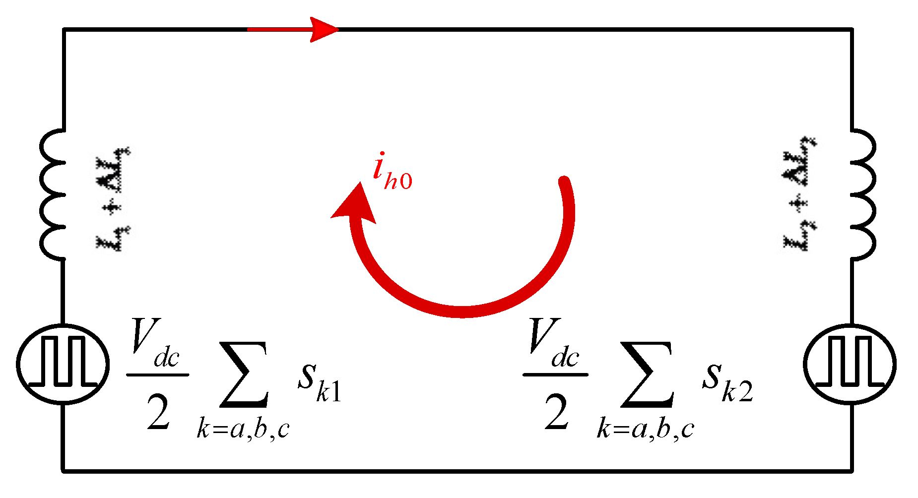
Firstly, a ZSCC mathematical model and an equivalent ZSCC circuit model incorporating perturbations of the inductor parameters are developed.
(2)
Secondly, the inductance parameters are estimated online based on the EKF and the preset inductance parameters in the controller are updated in real time.
(3)
Finally, a ZSCC controller is implemented by using the EKF and fixed-time stability theory, which ensures that the system can suppress the ZSCC under different conditions.
The structure of this document is presented below. Part I summarizes the results and shortcomings that have been achieved in the current ZSCC suppression strategy. In part II, the ZSCC problem in parallel inverters system is introduced extensively, and the mathematical model between the ZSCC and zero vectors is established. In part III, based on the above numerical model, a fixed-time stable ZSCC controller is designed. Meanwhile, further improvements to the robustness of the controller will be made with the aim of enhancing its reliability, and an online estimation scheme of inductor parameters based on the EKF is designed. In part IV, experiments and simulations show that the proposed strategy works. In part V, the paper is concluded.

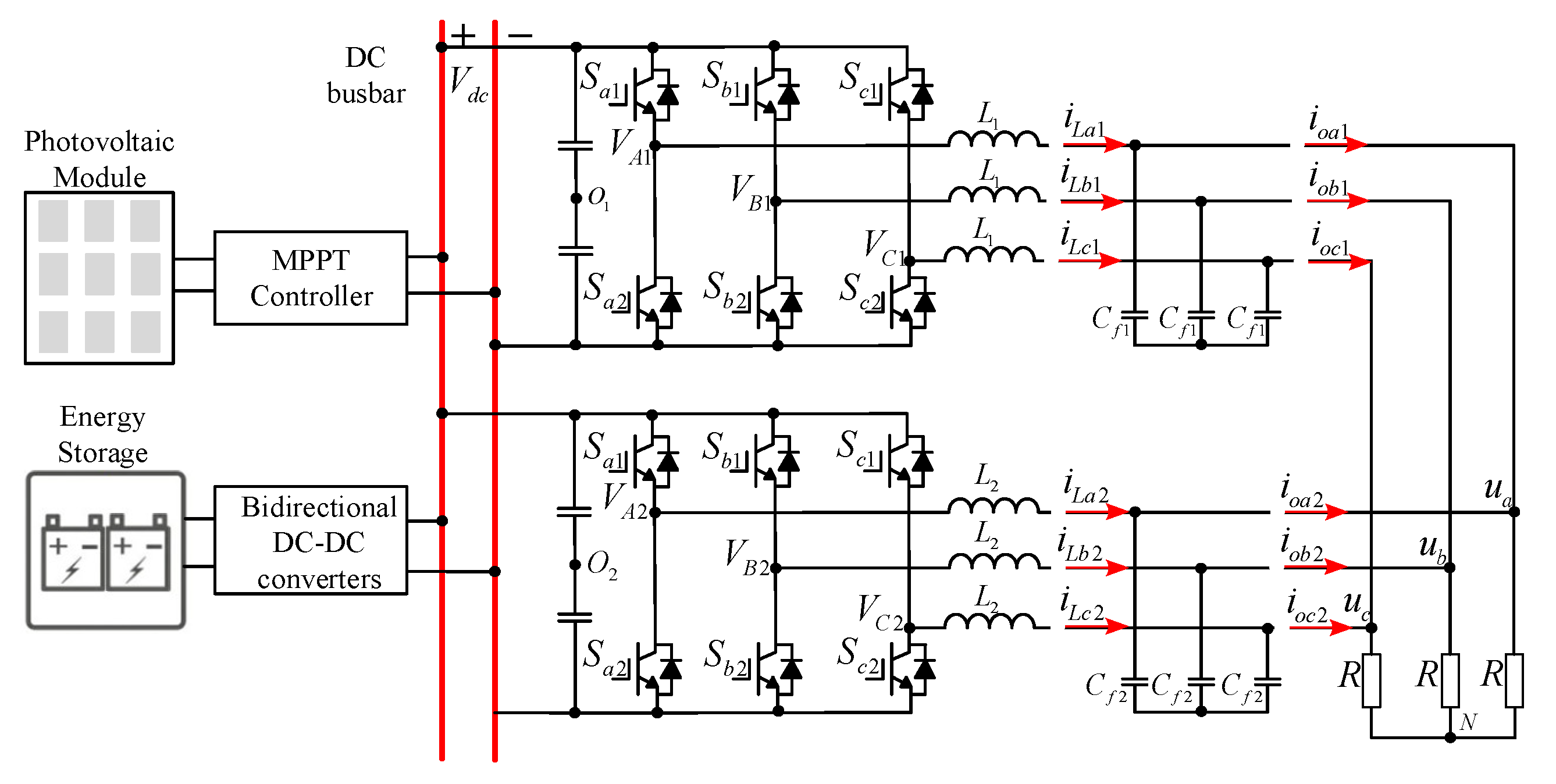
2. ZSCC Mathematical Modeling

To achieve a better performance of the ZSCC controller, this paper considers the ZSCC model in the case where the inductance parameters are consistent with the parameters pre-stored in the controller (hereinafter referred to as inductance parameter consistency) and in the case of inductance parameter perturbation.

2.1. Mathematical Modeling of ZSCC with Consistent Inductive Parameters

The topology of two inverters in parallel is depicted in Figure 1. In this configuration, the DC sides of both inverters are joined to the same DC bus, with the AC power supplies supplying the same load. The DC bus voltage is V d c , O j is the midpoint of the DC bus capacitance of the jth inverter, where j = ( 1 , 2 ) , j is the serial number of the inverter, and the following j has the same definition. L j is the filter inductor of the jth inverter, C f j is the filter capacitor of the jth inverter, i L k j is the current passing through the k-phase inductor of the jth inverter, k = ( a , b , c ) , k represents the three phase sequences of the inverter, and i o k j is the output current of the k-phase of the jth inverter.
The switching function is introduced to facilitate the description of the potential from the center of the inverter arm to the center of the DC side capacitor:
s k ( t ) = 1 A b o v e   IGBT   conduction 1 B e l o w   IGBT   conduction
In each inverter there are a total of two switching states for the IGBTs above each phase of the bridge arm, so there are a total of four switching states between the k-phase of the first inverter and the k-phase of the second inverter, including ( s k , 1 , s k , 2 ) = ( 1 , 1 ) , ( 1 , 1 ) , ( 1 , 1 ) and ( 1 , 1 ) . The circulation path of the circulating current is thus shown in Figure 2.
To establish a reference point for the DC-side capacitance, the midpoint was taken as the baseline for the subsequent calculations, and the inverter output voltage per phase of the bridge arm can be expressed as
V k O = V d c 2 s k
In accordance with the underlying symmetry of the three-phase system, we have V a N + V b N + V c N = 0 , and at the same time V k O = V k N + V N O , we can obtain the output voltage from the center of the load to the center of the DC bus:
V N O = V d c 6 k = a , b , c s k
In consequence of the KVL, the equation of the inverter loop voltage in its steady state can be expressed as follows:
L 1 d i L a 1 d t = V d c 2 s k V d c 6 k = a , b , c s k u a L 1 d i L b 1 d t = V d c 2 s k V d c 6 k = a , b , c s k u b L 1 d i L c 1 d t = V d c 2 s k V d c 6 k = a , b , c s k u c
L 2 d i L a 2 d t = V d c 2 s k V d c 6 k = a , b , c s k u a L 2 d i L b 2 d t = V d c 2 s k V d c 6 k = a , b , c s k u b L 2 d i L c 2 d t = V d c 2 s k V d c 6 k = a , b , c s k u c
where V A j , V B j , and V C j are the output voltages at the center of the inverter bridge arm; L 1 and L 2 are the filter inductors of the inverter, respectively; i L a j , i L b j and i L c j are the currents flowing through the filter inductor, respectively; u a , u b and u c are the voltages at the ends of the load and u N n is the voltage between the center N of the load and the negative terminal n of the DC bus. If the inverters are running in parallel with a common DC power supply and a common AC load, a loop current path is created in inverter 1 and inverter 2 to provide a circulation path for the loop current, as indicated Figure 2.
The loop current of inverters 1 and 2 can be defined as the distinction derived from the measured output current of each inverter and the average current of all inverters. According to the definition of loop current, it can be demonstrated that the loop current between inverters 1 and 2 is of equal magnitude and opposite direction. Therefore, Equation (6) be obtained.
i k h = i L k 1 i L k a v g = i L k 1 i L k 1 + i L k 2 2 = i L k 1 i L k 2 2
where i L K a v g represents the mean value of the kth phase current in the inverter, whereas i K h denotes the loop current of the kth phase bridge arm of the first inverter. It can be obtained from Equation (6):
i L k 1 = i L k a v g + i k h i L k 2 = i L k a v g i k h
From Equation (7) and the KCL, it is known that in the presence of circulating currents in the system of parallel inverters, the inductor and output currents of each inverter are not necessarily symmetrical, but the total current of the load is symmetrical.
If the loop currents in the parallel inverter system are considered and combined with Equations (4) and (5), new loop voltage equations for inverter 1 and inverter 2 can be obtained.
L 1 d ( i L k a v g + i k h ) d t + u k + V N O 1 = V d c 2 s k 1 L 2 d ( i L k a v g i k h ) d t + u k + V N O 2 = V d c 2 s k 2
Subtracting the two equations in Equation (8) gives the circulation in each phase as
( L 1 + L 2 ) d i k h d t = V d c 2 ( s k 1 s k 2 ) ( V N O 1 V N O 2 )
Equation (9) depicts the relationship between the magnitude of the loop current and two key parameters: the switching states of the corresponding phase inverters and the distinction among their common mode voltages. As the two inverters use the same DC and AC side, a path is created for the ZSCC, defined as the ZSCC, which can be described as follows:
i h 0 = k = a , b , c i k h = k = a , b , c i o k 1 = k = a , b , c i o k 2
In a three-phase symmetrical system, the voltage between the center of the load and the center of the capacitor on the DC side is the same, so there is V O 1 N = V O 2 N , hence the ZSCC can be described as
( L 1 + L 2 ) d i h 0 d t = V d c 2 ( k = A , B , C s k 1 k = A , B , C s k 2 )

2.2. Mathematical Modeling of ZSCC in Case of Perturbation of Inductive Parameters

From Equation (11), it is seen that the ability of the ZSCC controller to suppress the ZSCC is highly dependent on the inductance parameter, and an unknown or disturbed inductance parameter will have a negative correlation on the accuracy, stability, and speed of the ZSCC controller. The model of the ZSCC can be rewritten when the inductance parameter is disturbed.
( L 1 + L 2 ) d i h 0 d t = V d c 2 ( k = A , B , C s k 1 k = A , B , C s k 2 )
where L 1 and L 2 are L 1 + Δ L 1 and L 2 + Δ L 2 , respectively, and Δ L is the deviation of the inductance.
According to Equation (12), the corresponding circuit diagram of the ZSCC can be obtained as depicted in Figure 3.
According to Equation (11), the amplitude characteristic of the ZSCC controller at different inductance parameters can be obtained as shown in Figure 4. To illustrate the effect of inductive disturbances on the ZSCC controller, define K = L / L .
In Figure 4, it is obvious that when the inductance parameter is perturbed, it will have an effect on the bandwidth of the ZSCC controller and hence on the stability of the ZSCC. From Equation (11), it can be seen that the magnitude of the ZSCC is related to the amplitude of the DC-side voltage, the parameters of the inductor in the filter, and the switching state. To facilitate subsequent analysis, the inverter’s zero sequence state is described as follows:
s 0 = k = A , B , C s k
Thus, by combining Equations (11) and (13), the association amongst the ZSCC, the zero sequence switching state and the aforementioned relationship is defined as follows:
2 ( L 1 + L 2 ) d i h 0 d t = V d c 2 ( s 10 s 20 )
From Equation (14), the ZSV corresponding to the ZSCC is obtained as
u h 0 = V d c 2 ( s 10 s 20 )
The duty cycle that corresponds to the ZSCC of the inverter could be described as follows:
d 0 j = d A j + d B j + d C j
Combining Equations (11) and (15) gives the transfer function of the ZSCC, which is displayed as follows:
G h 0 s = i h 0 s u h 0 s = 1 ( L 1 + L 2 ) s
In the inverter control, the desired voltage vector of SVPWM is determined by the result of the calculation performed by the current loop controller. In the interrupt procedure, the reference voltage vector is employed to ascertain the sector in which the synthesized vector is situated. It calculates the adjacent vector action time, calculates the on-time of each bridge arm, and then calculates the duty cycle, and, of the three phases of the inverter, it finally updates the corresponding register values, as shown in Figure 5. The action of the zero vector does not impact the synthesis of the reference voltage vector. The selection of the zero-vector factor allows for the greatest flexibility, and an optimal zero vector can result in a reduction in the number of switching times, a decrease in switching at moments of high load current, and a reduction in switching losses. Appropriate allocation of the time of action of the zero vector can change the magnitude of the ZSV and thus suppress the ZSCC in the parallel inverter system.
In a switching cycle, the action times of the non-zero vectors are determined as d A , d B , and d B , respectively, and d 0 is defined as the Zero Sequence Duty Cycle (ZSDC). Introducing the zero-vector assignment adjustment factor u , the configuration of the switching states within a single switching cycle is illustrated in Figure 5.
According to Figure 6, the sum of the non-zero vectors of the ABC three phases of each inverter can be calculated as
d A j + d B j + d C j = ( d 1 j + d 2 j + d 0 j 2 2 u j ) + ( d 2 j + d 0 j 2 2 u j ) + ( d 0 j 2 2 u j ) = d 1 j + 2 d 2 j + 3 ( d 0 j 2 2 u j )
According to Equation (10), it can be known that the ZSCC of each inverter in the parallel inverter system is the same in magnitude and opposite in direction, so when designing the ZSCC controller, it is sufficient to redistribute the zero sequence time in a single inverter. The duty cycle of zero vectors and the duty cycle of non-zero vectors in each phase during a switching cycle satisfy
d 1 + d 2 + d 0 = 1
Therefore, combining Equations (16), (18), and (19), the distinction regarding the ZSDC of the two inverters can be established through the following calculation:
s 10 s 20 = ( d A 1 + d B 1 + d C 1 ) ( d A 2 + d B 2 + d C 2 ) = d 11 + 2 d 21 + 3 ( d 01 2 2 u 1 ) d 22 2 d 22 3 d 02 2 = 1 2 ( d 22 d 11 + d 21 d 12 ) + 6 u 1
Bringing Equations (20) and (15) into Equation (17) and simplifying can obtain the relationship between zero-vectors and ZSCC as
i h 0 = 6 u ( s ) V d c ( L 1 + L 2 ) s + Δ d V d c 2 ( L 1 + L 2 ) s
where Δ d = d 22 d 11 + d 21 d 12 is the perturbation due to uneven power sharing between the two inverters.

3. ZSCC Controller Design

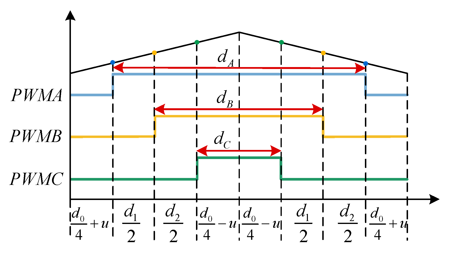
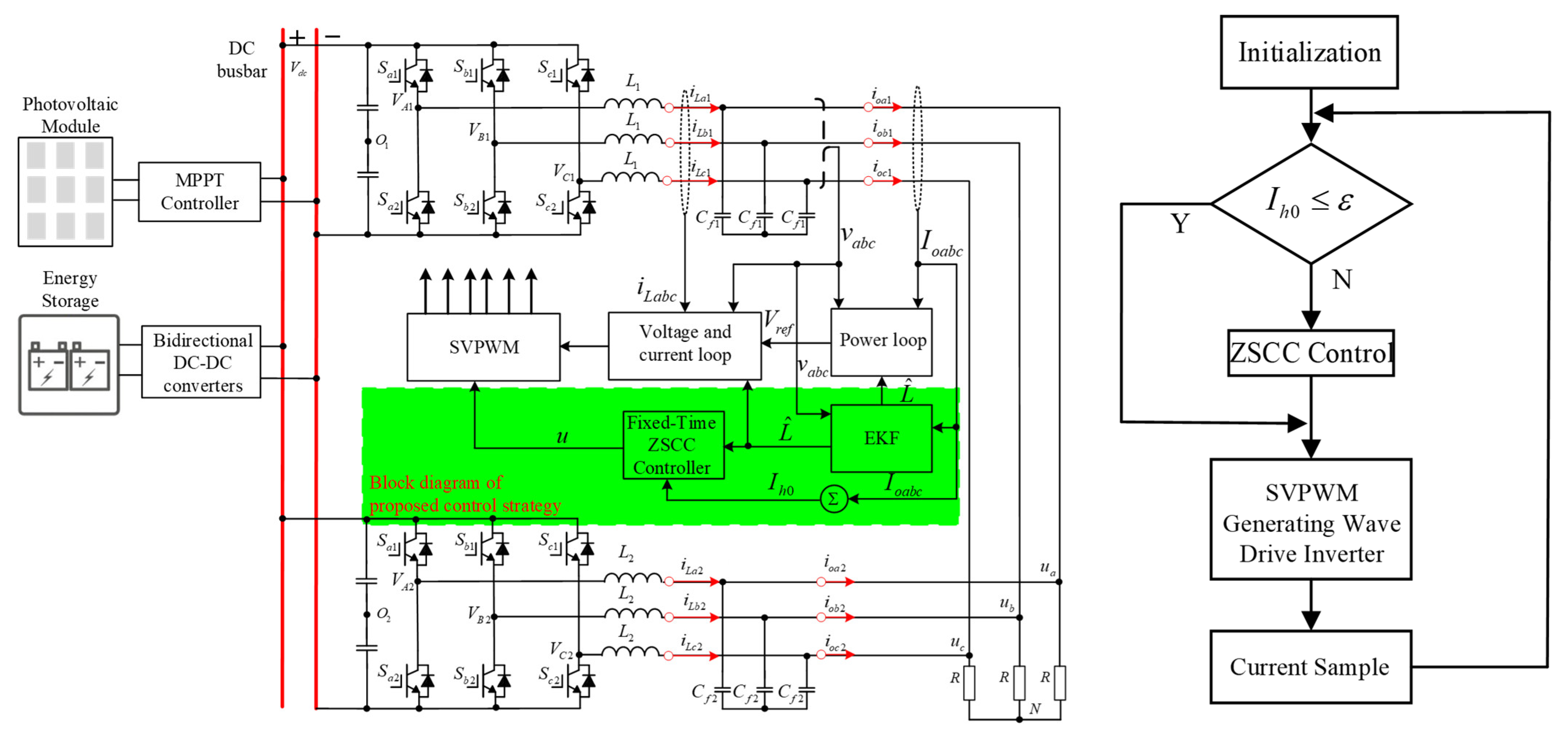
3.1. Control Scheme of the System Under the Control Approach Presented in This Study

Figure 7 presents the control schematic of the ZSCC suppression strategy adopted in this study for a parallel inverter system. It can be seen that the front stage of the system consists of the PV and the energy storage system, which are jointly linked to a DC bus shared by the inverters in the backstage, and the AC output of the inverters can supply the loads. From Figure 7, it is apparent that based on the traditional inverter control scheme, a ZSCC detection module, a fixed-time ZSCC controller, and an EKF are added. The working principle is as follows: first, the ZSCC and the corrected inductance parameters in the system are detected, then the zero vector assignment factor u is calculated in the fixed-time ZSCC controller, and finally the control signal for the IGBT is generated by the SVPWM module.

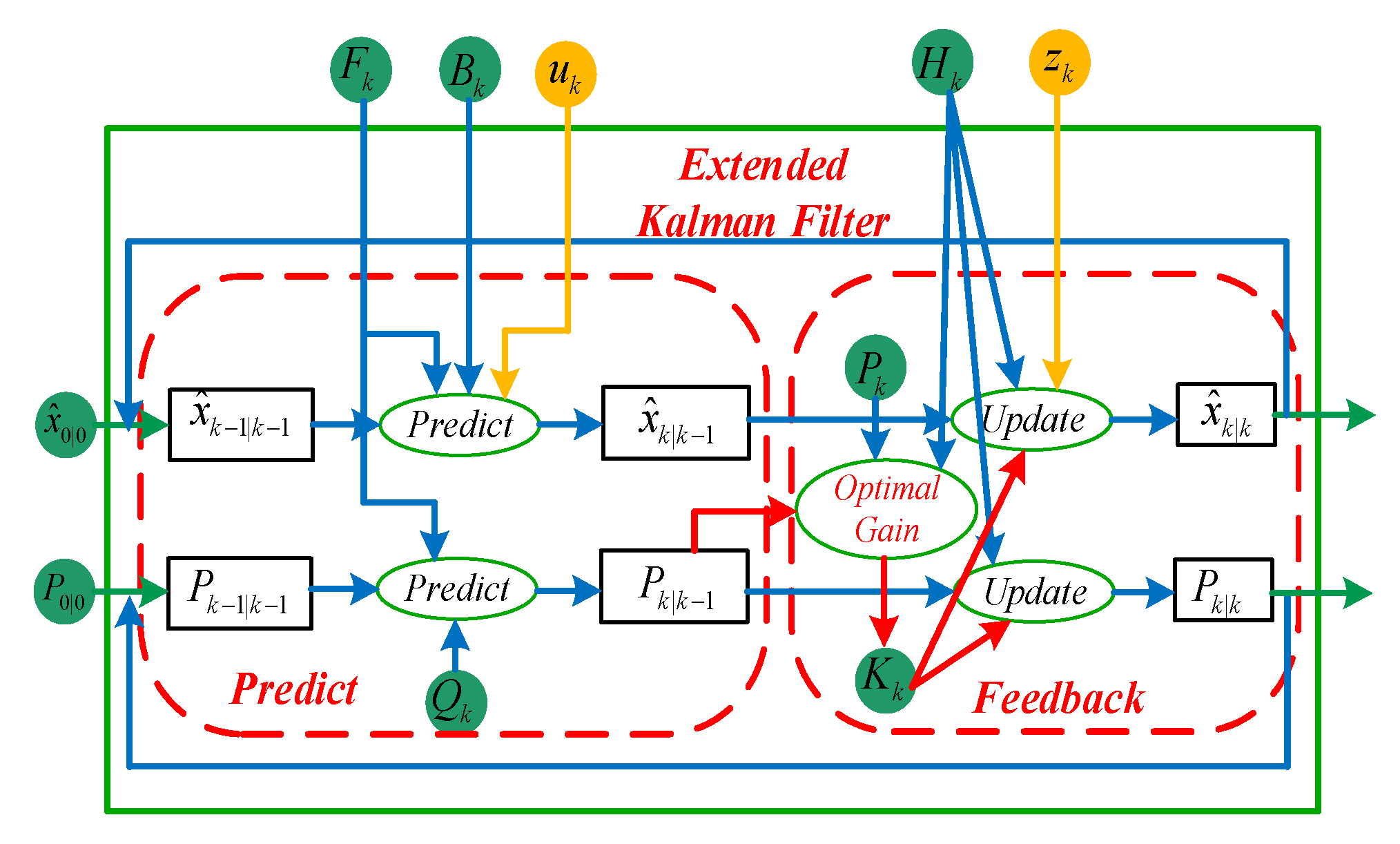
3.2. Extended Kalman Filter-Based Inductor Parameter Identification for Inverters

To solve the problem of the deterioration of the ZSCC suppression effect due to the change in the inductance parameter in the traditional ZSCC suppression strategy, this paper adopts the EKF for the estimation of the inductance parameter, which further improves the robustness of the controller. The fundamental principle of the EKF is the minimization of mean variance, achieved through an iterative process comprising two stages, prediction and feedback, and its working principle is displayed in Figure 8. According to Figure 1, the mathematics model of inverter 1 in the dq coordinate system is as follows:
L 1 d i d d t = i d R + ν d ν L d + i q ω L 1 L 1 d i q d t = i q R + ν q ν L q i d ω L 1
where v d , v q , i d , i q , v L d , v L q , R , L 1 , and ω are the output voltage of the bridge arm of the inverter, the current flowing through the inductor, the voltage of the load, the Equivalent Series Resistance (ESR) of the inductor, the value of the inductance of the filter, and the angular frequency, and the inductance and the angular frequency, respectively, of the filter, in the dq coordinate system. For descriptive convenience, define u d = v d v L d , u q = v q v L q .
The state and measuring equations of a nonlinear system in a continuous state can be described as follows:
x k = f ( x k 1 , u k 1 , w k 1 ) y k = h ( x k , v k )
where x k and x k 1 are the current and previous values of the state variables, respectively, u k 1 is the input to the system, ω k 1 and v k are the noise and measurement noise of the system, and y k is the output of the system.
Since the control period T s is very short, it can be assumed that the parameter of the inductor L is not found to change during a control period. Therefore, the EKF state equation in discrete form can be constructed by combining Equations (22) and (23) as follows:
x k = ϕ k 1 x k 1 + w k 1 y k = H k x k 1 + ν k 1
where a = 1 / L . According to Equation (24), the Jacobi matrix and the state transfer matrix in Equation (24) can be known as follows:
H k = h x | x = x ^ k = 1 0 0 0 1 0
ϕ k 1 = I + f x | x = x ˙ k 1 T s = 1 a R T s ω T s ( u d R i d ) T s ω T s 1 a R T s ( u q R i q ) T s 0 0 1
Assuming that the value x ^ k 1 of the state variable and the value P k 1 of the covariance matrix at the previous moment are known, the prediction process of the EKF without considering system noise is
x ^ k / k 1 = f ( x ^ k 1 , u k 1 ) P k / k 1 = F k 1 P k 1 F K 1 T + Q K 1
where F k 1 = f x x = x ^ k 1 ; Q K 1 = cov ( ω k 1 ) . Through Equation (27), the predicted values of the state variables at this moment and the predicted values of the covariance matrix can be obtained. Therefore, the correction process of the EKF is
K k = P k / k 1 H k T ( H k P k / k 1 H k T + R k ) 1 x ^ k = x ^ k / k 1 + K k ( y k H ( x ^ k / k 1 ) ) P k = ( I K k H k ) P k / k 1
where H k = h x x = x ^ k 1 ; R k = cov ( v k ) . The Kalman gain matrix K k can be calculated by Equation (28), the state variable x ^ k can be calculated from the observation y k and the corrected state prediction x ^ k / k 1 . Finally, the updated value of the corrected covariance matrix P k is obtained.
In practical engineering applications, the presence of process noise in the system model and the measurement of system interference noise during the process cannot be directly determined. In several debugging scenarios, the selection of optimal parameters for parameter estimation is crucial. In such cases, the values of P , Q , and R are d i a g 0.1   0 . 1   10 , d i a g 1   1   5 , and d i a g 0.08   0 . 08 , respectively.
Bringing Equations (25) and (26) into Equations (27) and (28) for iteration, the intermediate variable a can be obtained, and finally the estimated value of the filter inductance parameter is given by L ^ = 1 / a ^ .

3.3. Design of ZSCC Controller Based on Fixed-Time Stabilization Theory

Definition 1.
Suppose there exists a nonlinear system with an origin of equilibrium as shown in Equation (29):
x ˙ = h ( t , x ) , x ( 0 ) = x 0
where  x n  is the state vector of the system and  h : n n  is a nonlinear function vector. If there exists a finite convergence time  t s , then  x ( t ) = 0  holds constant when  T > t s , and the system (29) is finite-time stable.
Definition 2
([24]). Suppose the system is finite-time stable. If there exists a convergence time  t s  independent of the state of the system, then the system is fixed-time stable.
Lemma 1.
Consider  V ( x )  to be a smooth function which at the same time satisfies  V ( x ) 0 . If Equation (30) is satisfied, then the origin ( x = 0 ) of the system (29) is stable in fixed time and the maximum finite convergence time  t s  is given in Equation (31).
V ˙ ( x ) μ 1 V ( x ) α μ 2 V ( x ) β + δ
t s t s max 1 κ 1 ( 1 α ) + 1 κ 2 ( β 1 )
where μ1, μ2, α, β are constants and  α ( 0 , 1 ) ,  β ( 1 , ) .
Equation (30) can be obtained from Equation (20).
d i h 0 ( t ) d t = 6 V d c L ^ 1 + L ^ 2 u ( t ) + V d c 2 ( L ^ 1 + L ^ 2 ) Δ d
where L ^ 1 and L ^ 2 are the inductance values calculated by the EKF estimation. The distinction between the target value and the measured value of the ZSCC, which is known as the tracking error, must be defined e = i h 0 r e f i h 0 , so that Equation (32) can be written as
d e ( t ) d t = 6 V d c L ^ 1 + L ^ 2 u ( t ) V d c 2 ( L ^ 1 + L ^ 2 ) Δ d + d i h 0 r e f d t
Based on the fixed-time stabilization theory of suppression, the input u to the ZSCC controller can be set.
u ( t ) = k 1 s i g ( e ( t ) ) α + k 2 s i g ( e ( t ) ) β
where s i g ( e ( t ) ) α = e ( t ) α s g n ( e ( t ) ) , sgn ( x ) is the sign function and the positive real numbers k 1 , k 2 are the gains of the fixed time ZSCC controller. Inserting Equation (34) into Equation (33), and also the controller’s objective is e 0 , i h 0 r e f = 0 can be obtained as
d e ( t ) d t = 6 V d c L ^ 1 + L ^ 2 k 1 s i g ( e ( t ) ) α + k 2 s i g ( e ( t ) ) β V d c 2 ( L ^ 1 + L ^ 2 ) Δ d

3.4. Proven Stability of ZSCC Controller

The Lyapunov function is chosen to be V = 0.5 e 2 according to the Lyapunov stability requirement, such that
V ˙ = e e ˙ = e ( t ) 6 V d c L ^ 1 + L ^ 2 k 1 s i g ( e ( t ) ) α + k 2 s i g ( e ( t ) ) β V d c 2 ( L ^ 1 + L ^ 2 ) Δ d
In this paper, the two parallel inverters have the same parameters, and the perturbations caused by the non-zero vectors are small enough to be obtained.
V ˙ e ( t ) 6 V d c L ^ 1 + L ^ 2 k 1 e ( t ) α 6 V d c L ^ 1 + L ^ 2 k 2 e ( t ) β + V d c 2 ( L ^ 1 + L ^ 2 ) Δ d 6 V d c L ^ 1 + L ^ 2 k 1 e ( t ) α + 1 6 V d c L ^ 1 + L ^ 2 k 2 e ( t ) β + 1 + V d c 2 ( L ^ 1 + L ^ 2 ) Δ d e ( t ) 2 1 + α 2 6 V d c L ^ 1 + L ^ 2 k 1 V 1 + α 2 2 1 + β 2 6 V d c L ^ 1 + L ^ 2 k 2 V 1 + β 2
From the Lemma 1 and Equation (30), it is known that the ZSCC controller designed in this paper is fixed-time stable and also from Equation (31) it is known that the upper limit of the stabilization period is as follows:
T max 1 κ 1 ( 1 α ) + 1 κ 2 ( β 1 ) = 1 2 1 + α 2 6 V d c L ^ 1 + L ^ 2 ( 1 1 + α 2 ) + 1 2 1 + β 2 6 V d c L ^ 1 + L ^ 2 ( 1 + β 2 1 )

4. Simulation and Experimentation

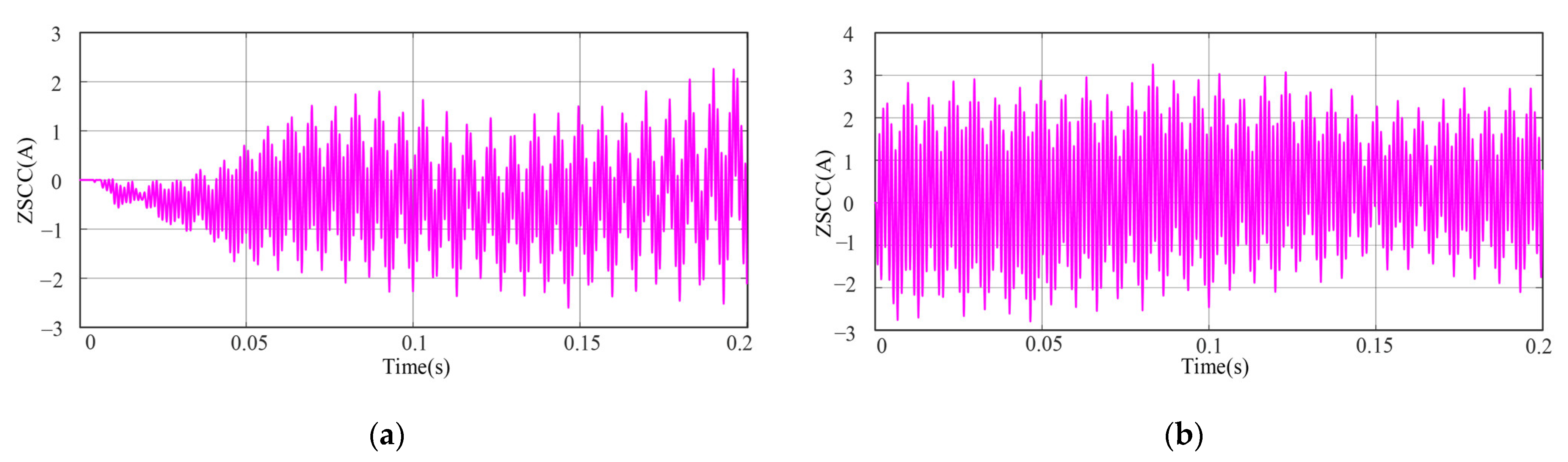
4.1. Simulation Verification

To verify the efficiency of the fixed-time ZSCC rejection methods proposed in this study, a system comprising two parallel inverters was constructed using MATLAB(2022a)/Simulink for the purpose of conducting a verification simulation. The parameters of the controller are taken as k 1 = 0.15 , k 2 = 0.2 , α = 0.5 , β = 2 . The simulation parameters of the inverter model are given in Table 1. The simulations are used to analyze the capabilities of the presented controller to suppress the ZSCC.
The ZSCC in the parallel inverter system is displayed in Figure 9. Since the ZSCC is not controlled, a great number of ZSCCs exist in the parallel inverter system, especially when the inductance parameter is disturbed, the amplitude of the ZSCC will increase, as shown in Figure 9b.
The spectrograms of the ZSCC show that the ZSCC in the parallel inverter system mainly contains harmonic components of the 3n (1, 3, 5 … (2m − 1)) harmonics, as indicated in Figure 10. In addition, the DC component in the ZSCC also has a large proportion. The presence of these harmonics causes serious distortion of the inverter output current, which is a major threat to the stable operation of the inverter parallel system.
The presence of the ZSCC has a major effect on the power quality of the inverter output, resulting in the distortion of the output current of the parallel inverters. The THD of the first inverter output current is 4.91% and 9.35% in the case of constant inductance parameter and in the case of inductance parameter disturbance, respectively, as indicated in Figure 11a,b.
From the spectrum of the inverter output current, when the inductor parameters are disturbed, the harmonic content of all frequency bands increases significantly.
After adding the ZSCC control scheme presented in this study at 0.1 s, the output currents of the first inverter in the case of consistent inductance parameters and in the case of occurrence of inductance parameter perturbation are displayed in Figure 12a,b. From Figure 12, it is observed that after the addition of the ZSCC suppression strategy proposed in this study at 0.1 s, the ZSCC is explicitly suppressed, the THD of the first inverter output current after reaching the steady state is 0.47% and 0.59%, and the harmonic content of each frequency band is obviously suppressed, as displayed in Figure 12c,d.
For the verification of the dynamic and stability capability of the design of the ZSCC control strategy in this study, a comparison with the ZSCC control scheme under the traditional PI controller is illustrated in Figure 13.
The ZSCC with consistent inductance parameters is depicted in Figure 13a,b, and the ZSCC with perturbed inductance parameters is illustrated in Figure 13c,d.
With the same inductance parameters, the conventional control strategy is added to the parallel inverter system at 0.1 s. After 0.05 s, the amplitude of the ZSCC is tremendously reduced, and finally the amplitude of the ZSCC is stabilized within the range of ±0.5 A, as illustrated in Figure 13b. The control strategy presented in this study is injected into the parallel inverter system at 0.1 s, and the ZSCC is quickly suppressed with a small steady-state error, as illustrated in Figure 13a.
In the case of inductance parameter disturbance, the amplitude of ZSCC is suppressed within the range of plus or minus 0.5 A after 0.2 s with the conventional control strategy added to the parallel inverter system at 0.1 s, as indicated in Figure 13d. In addition, the ZSCC is suppressed quickly with a small steady-state error using the proposed control scheme added to the parallel inverter system at 0.1 s, as depicted in Figure 13c. The comparative analysis demonstrates that the ZSCC control strategy, as proposed in this study, exhibits superior dynamic and stability performance compared to the traditional control strategy.
For mitigation of the effects of parameter changes on the ZSCC controller, an EKF is employed to identify the inductor of the inverter in a dynamic manner. The simulation outcomes are illustrated in Figure 14. The actual value of the inductance parameter is set to 3 mH, and following the initiation of the EKF algorithm, the estimation of the inductance is compared with the actual value in 0.01 s. The tracking process is rapid and exhibits minimal overshooting, with a maximum estimation error of less than 0.1%.
The effectiveness of the ZSCC control strategy proposed in this paper under more extreme conditions, i.e., when the inductance of phase-to-phase inductance imbalance, is verified. The simulation results of the phase-to-phase inductance imbalance are shown in Figure 15.
From Figure 15, the ZSCC in the inverter parallel system increases significantly when the phase-to-phase inductance imbalance occurs compared to Figure 13, and the output current of the first inverter undergoes more severe waveform distortion. At 0.1 s, after the ZSCC control strategy proposed in this paper is added, the ZSCC is quickly suppressed and, at the same time, the waveform of the output current of the first inverter is greatly improved.
At 0.1 s and 0.15 s, the load is abruptly changed to twice the rated load and the rated load, respectively. The output current of the first inverter changes from the original 10 A to 20 A at 0.1 s and from 20 A to 10 A at 0.15 s, as shown in Figure 16a. During the load switching process, the three-phase current output from the first inverter is not likely to reach the new steady state in an instant, thus causing the change in the ZSCC in the system at 0.1 s and 0.15 s load switching as shown in Figure 16b. However, with the ZSCC suppression strategy proposed in this paper, the ZSCC in the system is quickly suppressed after about half an industrial frequency cycle.

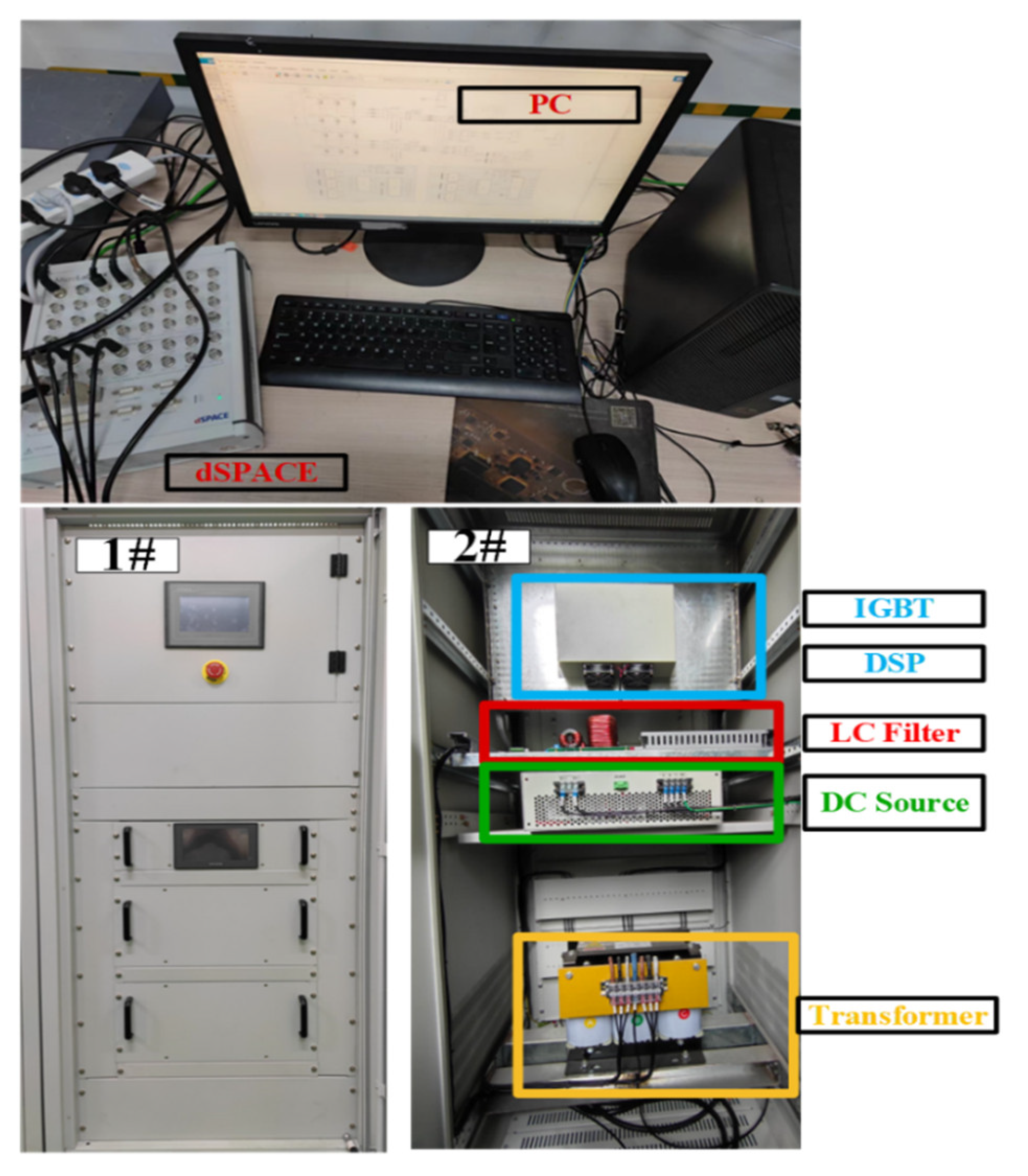
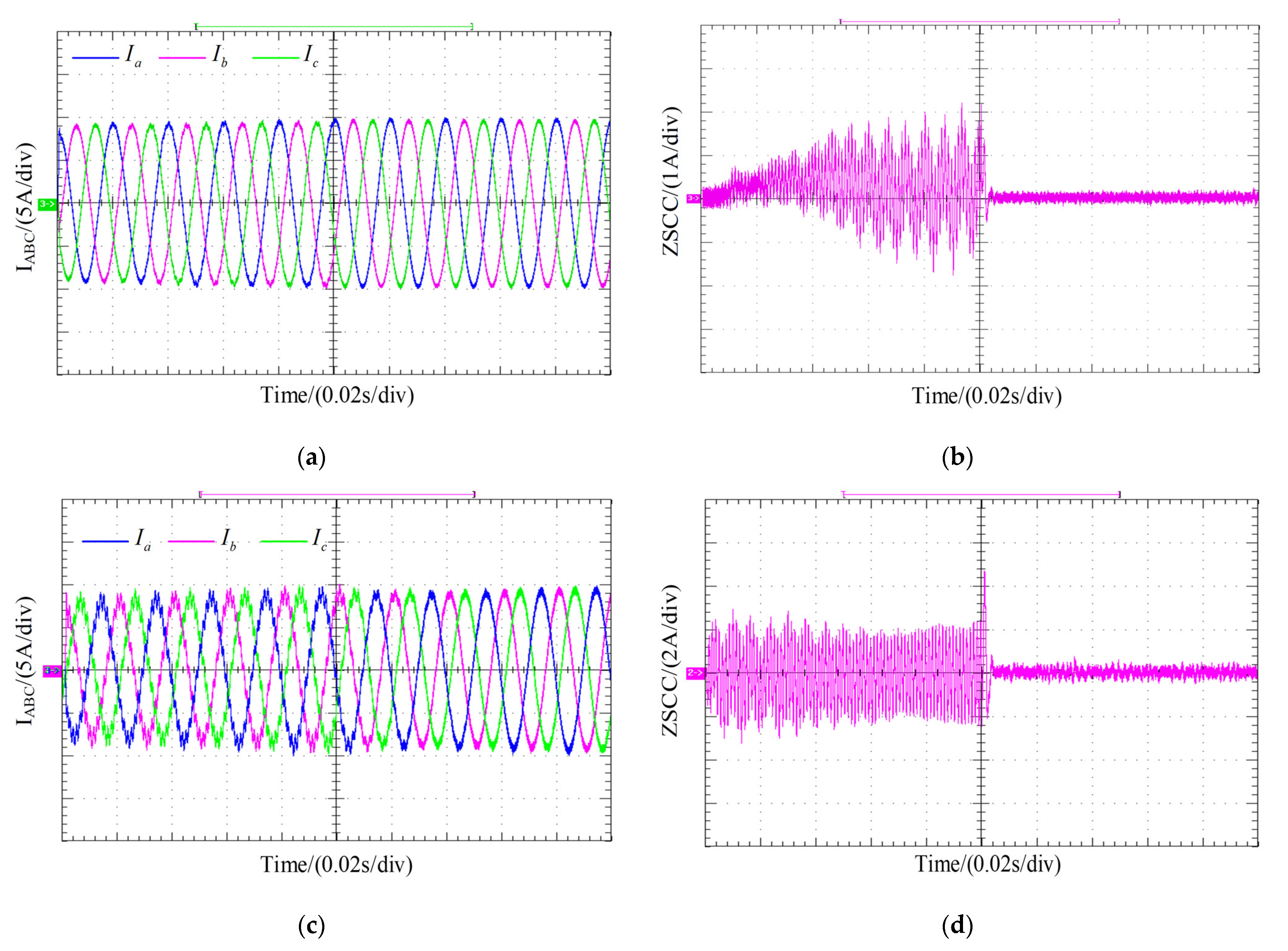
4.2. Experimental Validation

To further evaluate the applicability of the methodology in this study, the algorithm proposed in this study has been applied to the experimental prototype of the parallel inverters, as illustrated in Figure 17.
The system is tested through hardware-in loop (HIL). The physical verification of the parallel inverter system is performed using the dSPACE1202 system. The dSPACE1202 controller is used to generate digital drive pulses, which are amplified by the driver to apply the drive signals to the IGBTs. The current and voltage generated by the inverter are connected to the internal ADC module of the dSPACE1202 via the voltage–current sampling circuit to complete the closed-loop control.
Figure 18 illustrates the current waveform of the first inverter output when two three-phase inverters are operated in parallel. Before 0.1 s, the inverter output current is distorted due to the presence of the ZSCC, and when the inductance parameter is perturbed, the ZSCC has a greater effect on the output current quality, as illustrated in Figure 18a,c. After adding the ZSCC rejection strategy presented in this study at 0.1 s, the ZSCC is quickly eliminated, and the quality of the inverter output current is dramatically better than before 0.1 s, as illustrated in Figure 18b,d.

5. Conclusions

Aiming at the problem of the ZSCC in parallel inverter system, a fixed-time ZSCC suppression method that relies on an EKF is proposed. By building the mathematical model of the ZSCC and the model of the observed inductance of the EKF, the design process of the proposed control scheme is worked out in detail and the system is proved to be stable in fixed time. By comparing the simulation and experimental results with the steady state and dynamics under the conventional ZSCC suppression strategy, the following is a summary of the conclusions that can be reached.
(1)
Compared with the conventional ZSCC control strategy, the proposed control strategy takes into account the effect of filter parameter perturbations and improves the robustness of the system by extending the Kalman filter to predict the inductance.
(2)
The proposed control strategy can suppress the ZSCC in parallel inverters system faster than the traditional ZSCC control strategy.
(3)
Under the proposed control strategy, for the ZSCC during parallel operation, the inverter parallel inverters system can respond quickly to the suppression of the ZSCC and the suppression effect of the inverters on the ZSCC, and there is no correlation between the time to stabilization and the state of the system, which improves the dynamic performance of the system.

Author Contributions

Conceptualization, G.H. and X.L.; methodology, X.L. and G.H.; software, X.L. and G.H.; validation, X.L. and Y.Z.; formal analysis, X.L. and Y.Z.; investigation, X.L.; resources, G.H.; data curation, X.L.; writing—original draft preparation, X.L. and G.H.; writing—review and editing, X.L., H.W. and G.H.; visualization, Y.Z.; supervision, G.H.; project administration, G.H. and Y.D. All authors have read and agreed to the published version of the manuscript.

Funding

This research was funded by Henan Province, China, grant number 24210230202. The project name is Research and Application of Key Technology of Active Disturbance Rejection Control for Shunt Active Power Filter. The project host is Dong Yanfei.

Data Availability Statement

The data presented in this research study are available in this article.

Conflicts of Interest

The authors declare no conflicts of interest.

Nomenclature

Zero Sequence VoltageZSVDC Bus Voltage V d c Output Current i o k j
Zero Sequence PathZSPThe midpoint of the DC bus O j Inverter Output Voltage V A j V B j V C j
Zero Sequence Circulating CurrentZSCCFilter Capacitor C f j Load Voltage u a , u b , u c
Extended Kalman FilterEKFCurrent passing through the inductor i L k j Neutral Voltage u N n
Distributed Generation systemDGsFilter Inductor L j D-axis Q-axis Voltage v d , v q
Total Harmonic DistortionTHDLoad R D-axis Q-axis Current i d , i q
Zero Sequence Duty CycleZSDCInitial Covariance Matrix P Process Noise Covariance Q
Measurement Noise Covariance R Inductance Estimate L ^ 1 L ^ 2 Current Values x k
Previous Values x k 1 Input to the system u k 1 System Noise ω k 1
Measurement noise v k Output of the system y k Control period T s

References

  1. Zhuo, Z.; Zhang, N.; Xie, X.; Li, H.; Kang, C. Key technologies and developing challenges of power system with high proportion of renewable energy. Autom. Electr. Power Syst. 2021, 45, 171–191. [Google Scholar]
  2. Zhang, H.; Xiang, W.; Lin, W.; Wen, J. Grid Forming Converters in Renewable Energy Sources Dominated Power Grid: Control Strategy, Stability, Application, and Challenges. J. Mod. Power Syst. Clean Energy 2021, 9, 1239–1256. [Google Scholar] [CrossRef]
  3. Ebinyu, E.; Abdel-Rahim, O.; Mansour, D.-E.A.; Shoyama, M.; Abdelkader, S.M. Grid-Forming Control: Advancements towards 100% Inverter-Based Grids—A Review. Energies 2023, 16, 7579. [Google Scholar] [CrossRef]
  4. Chen, Z.; Li, X.; Xing, X.; Fu, Y.; Zhang, B.; Pang, X.; Zhang, C. The Tolerance Control Method Based on Zero-Sequence Circulating Current Suppression for Parallel T-Type Three-Level Rectifiers. IEEE J. Emerg. Sel. Top. Power Electron. 2022, 10, 4383–4394. [Google Scholar] [CrossRef]
  5. Wang, X.; Zou, J.; Zhao, J.; Xie, C.; Li, K.; Munir, H.M.; Guerrero, J.M. A Novel Model Predictive Control Strategy to Eliminate Zero-Sequence Circulating Current in Paralleled Three-Level Inverters. IEEE J. Emerg. Sel. Top. Power Electron. 2019, 7, 309–320. [Google Scholar] [CrossRef]
  6. Pan, C.-T.; Liao, Y.-H. Modeling and Coordinate Control of Circulating Currents in Parallel Three-Phase Boost Rectifiers. IEEE Trans. Ind. Electron. 2007, 54, 825–838. [Google Scholar] [CrossRef]
  7. Liu, X.; Liu, T.; Chen, A.; Xing, X.; Zhang, C. Circulating Current Suppression for Paralleled Three-Level T-Type Inverters with Online Inductance Identification. IEEE Trans. Ind. Appl. 2021, 57, 5052–5062. [Google Scholar] [CrossRef]
  8. Li, Z.; Nie, Z.; Ai, S. Nonlinear Modeling and Improved Suppression of Zero-Sequence Circulating Current for Parallel Three-Level Inverters. IEEE J. Emerg. Sel. Top. Power Electron. 2023, 11, 3036–3049. [Google Scholar] [CrossRef]
  9. Simanjorang, R.; Miura, Y.; Ise, T.; Sugimoto, S.; Fujita, H. Application of Series Type BTB Converter for Minimizing Circulating Current and Balancing Power Transformers in Loop Distribution Lines. In Proceedings of the 2007 Power Conversion Conference—Nagoya, Nagoya, Japan, 2–5 April 2007; pp. 997–1004. [Google Scholar] [CrossRef]
  10. Inzunza, R.; Sumiya, T.; Fujii, Y.; Ikawa, E. Parallel connection of grid-connected LCL inverters for MW-scaled photovoltaic Systems. In Proceedings of the 2010 International Power Electronics Conference—ECCE ASIA, Sapporo, Japan, 21–24 June 2010; pp. 1988–1993. [Google Scholar] [CrossRef]
  11. Sato, Y.; Kataoka, T. Simplified control strategy to improve AC-input-current waveform of parallel-connected current-type PWM rectifiers. IEE Proc.-Electr. Power Appl. 1995, 142, 246–254. [Google Scholar] [CrossRef]
  12. Zhang, D.; Wang, F.; Burgos, R.; Boroyevich, D. Common mode circulating current control of interleaved three-phase two-level voltage-source converters with discontinuous space-vector modulation. In Proceedings of the 2009 IEEE Energy Conversion Congress and Exposition, San Jose, CA, USA, 20–24 September 2009; pp. 2801–2807. [Google Scholar] [CrossRef]
  13. Ye, Z.; Boroyevich, D.; Choi, J.-Y.; Lee, F.C. Control of circulating current in two parallel three-phase boost rectifiers. IEEE Trans. Power Electron. 2002, 17, 609–615. [Google Scholar] [CrossRef]
  14. Son, Y.-K.; Chee, S.-J.; Lee, Y.; Sul, S.-K.; Lim, C.; Huh, S.; Oh, J. Suppression of Circulating Current in parallel operation of three-level converters. In Proceedings of the 2016 IEEE Applied Power Electronics Conference and Exposition (APEC), Long Beach, CA, USA, 20–24 March 2016; pp. 2370–2375. [Google Scholar] [CrossRef]
  15. Zhang, C.; Wang, Z.; Xing, X.; Li, X.; Liu, X. Modeling and Suppression of Circulating Currents Among Parallel Single-Phase Three-Level Grid-Tied Inverters. IEEE Trans. Ind. Electron. 2022, 69, 12967–12979. [Google Scholar] [CrossRef]
  16. Panprasert, D.; Neammanee, B. The d and q Axes Technique for Suppression Zero-Sequence Circulating Current in Directly Parallel Three-Phase PWM Converters. IEEE Access 2021, 9, 52213–52224. [Google Scholar] [CrossRef]
  17. Stonier, A.A.; Murugesan, S.; Samikannu, R.; Krishnamoorthy, V.; Subburaj, S.K.; Chinnaraj, G.; Mani, G. Fuzzy Logic Control for Solar PV Fed Modular Multilevel Inverter Towards Marine Water Pumping Applications. IEEE Access 2021, 9, 88524–88534. [Google Scholar] [CrossRef]
  18. Han, W. Research on Control Strategy of Vienna Rectifier and its Parallel System. Master’s Thesis, Shandong University, Jinan, China, 2023. [Google Scholar]
  19. Mohapatra, S.R.; Agarwal, V. Model Predictive Controller with Reduced Complexity for Grid-Tied Multilevel Inverters. IEEE Trans. Ind. Electron. 2019, 66, 8851–8855. [Google Scholar] [CrossRef]
  20. Sarrafan, N.; Zarei, J.; Razavi-Far, R.; Saif, M.; Khooban, M.-H. A Novel On-Board DC/DC Converter Controller Feeding Uncertain Constant Power Loads. IEEE J. Emerg. Sel. Top. Power Electron. 2021, 9, 1233–1240. [Google Scholar] [CrossRef]
  21. Komurcugil, H.; Ozdemir, S.; Sefa, I.; Altin, N.; Kukrer, O. Sliding-Mode Control for Single-Phase Grid-Connected LCL Filtered VSI with Double-Band Hysteresis Scheme. IEEE Trans. Ind. Electron. 2016, 63, 864–873. [Google Scholar] [CrossRef]
  22. Xu, Q.; Blaabjerg, F.; Zhang, C. Finite-time Stabilization of Constant Power Loads in DC Microgrids. In Proceedings of the 2019 IEEE Energy Conversion Congress and Exposition (ECCE), Baltimore, MD, USA, 29 September–3 October 2019; pp. 2059–2064. [Google Scholar] [CrossRef]
  23. Ahmad, A.; Ullah, N.; Ahmed, N.; Ibeas, A.; Mehdi, G.; Herrera, J.; Ali, A. Robust Control of Grid-Tied Parallel Inverters Using Nonlinear Backstepping Approach. IEEE Access 2019, 7, 111982–111992. [Google Scholar] [CrossRef]
  24. He, G.; Zhou, Z.; Zhang, G.; Li, G. Fixed-time fuzzy backstepping control strategy for islanded photovoltaic parallel inverters. Dianli Xitong Baohu Yu Kongzhi/Power Syst. Prot. Control 2023, 51, 147–156. [Google Scholar]
  25. Zhang, P.; Zhang, G.; Du, H. Circulating current suppression of parallel photovoltaic grid-connected converters. IEEE Trans. Circuits Syst. II Express Briefs 2018, 65, 1214–1218. [Google Scholar] [CrossRef]
  26. Wang, H.; Dong, Y.; He, G.; Song, W. Fixed-Time Backstepping Sliding-Mode Control for Interleaved Boost Converter in DC Microgrids. Energies 2024, 17, 5377. [Google Scholar] [CrossRef]
  27. Song, W.; Dong, Y.; He, G.; Zhou, Z. Fixed-Time Robust Fractional-Order Sliding Mode Control Strategy for Grid-Connected Inverters Based on Weighted Average Current. Energies 2023, 17, 4577. [Google Scholar] [CrossRef]
  28. Zhang, Y.; Jiao, J.; Liu, J. Direct Power Control of PWM Rectifiers with Online Inductance Identification Under Unbalanced and Distorted Network Conditions. IEEE Trans. Power Electron. 2019, 34, 12524–12537. [Google Scholar] [CrossRef]
  29. Mehreganfar, M.; Saeedinia, M.H.; Davari, S.A.; Garcia, C.; Rodriguez, J. Sensorless Predictive Control of AFE Rectifier with Robust Adaptive Inductance Estimation. IEEE Trans. Ind. Informatics 2019, 15, 3420–3431. [Google Scholar] [CrossRef]
  30. Wang, Q.; Wang, S.; Fu, J.; Li, Y.; Feng, J. Predictive Current Control for Permanent Magnet Synchronous Motor Based on Model Reference Adaptive System Parameter Identification. Electr. Mach. Control Appl. 2017, 44, 48–53. [Google Scholar]
  31. Song, W.; Ren, H.; Ye, H. Position Sensorless Control of Dual Three Phase Permanent Magnet Synchronous Motor Based on MRAS. Zhongguo Dianji Gongcheng Xuebao/Proc. Chin. Soc. Electr. Eng. 2022, 42, 11641173. [Google Scholar] [CrossRef]
  32. Liu, X.; Wang, X.; Fu, S.; Liang, L.; Huang, J. Inductance Identification of Permanent Magnet Synchronous Motor Based on Least Square Method. Electr. Mach. Control Appl. 2020, 47, 1–5. [Google Scholar] [CrossRef]
  33. Pasqualotto, D.; Rigon, S.; Zigliotto, M. Sensorless Speed Control of Synchronous Reluctance Motor Drives Based on Extended Kalman Filter and Neural Magnetic Model. IEEE Trans. Ind. Electron. 2023, 70, 1321–1330. [Google Scholar] [CrossRef]
  34. Gao, F.; Yin, Z.; Bai, C.; Yuan, D.; Liu, J. A Lag Compensation-Enhanced Adaptive Quasi-Fading Kalman Filter for Sensorless Control of Synchronous Reluctance Motor. IEEE Trans. Power Electron. 2022, 37, 15322–15337. [Google Scholar] [CrossRef]
  35. Hou, J.; Yang, Y.; Gao, T. A Variational Bayes Based State-of-Charge Estimation for Lithium-Ion Batteries Without Sensing Current. IEEE Access 2021, 9, 84651–84665. [Google Scholar] [CrossRef]
  36. Li, H.; Xu, H.; Xu, Y. Model prediction torque control of PMSM based on extended Kalman filter parameter identification. Electr. Mach. Control 2023, 19–30. [Google Scholar] [CrossRef]
  37. Yin, Z.; Li, G.; Zhang, Y.; Liu, J.; Sun, X.; Zhong, Y. A Speed and Flux Observer of Induction Motor Based on Extended Kalman Filter and Markov Chain. IEEE Trans. Power Electron. 2017, 32, 7096–7117. [Google Scholar] [CrossRef]
Figure 1. Inverter parallel topology.
Energies 18 00408 g001
Figure 2. A phase circulating current flow path of inverter parallel system.
Energies 18 00408 g002
Figure 3. The following diagrams represent the equivalence circuit for a ZSCC.
Energies 18 00408 g003
Figure 4. Closed-loop amplitude characteristic curve of ZSCC controller with different inductance parameters.
Energies 18 00408 g004
Figure 5. First sector ABC three-phase duty cycle action time plot.
Energies 18 00408 g005
Figure 6. Introducing a zero-vector assignment adjustment factor in a switching cycle switching state.
Energies 18 00408 g006
Figure 7. Control block diagram of the control scheme presented in this study for a parallel inverter system.
Energies 18 00408 g007
Figure 8. Working principle of EKF.
Energies 18 00408 g008
Figure 9. The ZSCC in inverter parallel system. (a) The ZSCC with constant inductance parameters; (b) the ZSCC in the presence of disturbances to the inductive parameters.
Energies 18 00408 g009
Figure 10. ZSCC harmonic spectrum in inverter parallel systems.
Energies 18 00408 g010
Figure 11. Inverter output current frequency spectrum. (a) Current spectrum of inverter output for consistent inductive parameters. (b) Inverter out current spectrum when inductance parameter disturbed.
Energies 18 00408 g011
Figure 12. Inverter output current after adding the ZSCC rejection strategy presented in this study at 0.1 s. (a) Inverter output current with consistent inductance parameters. (b) Inductor parameter perturbation in the case of inverter output current. (c) Spectrogram of inverter output current at steady state (with consistent inductor parameters). (d) Spectrogram of inverter output current at steady state (with inductive parameters perturbation).
Energies 18 00408 g012
Figure 13. The proposed control strategy in this paper and the conventional PI control strategy for the ZSCC in the inverter parallel system. (a) The ZSCC under the control strategy proposed in this paper with consistent inductance parameters; (b) the ZSCC under Pl control strategy with consistent inductance parameters; (c) the ZSCC under the control strategy proposed in this paper for inductance parameter perturbations; (d) the ZSCC under PI control strategy with inductive parameter perturbations.
Energies 18 00408 g013
Figure 14. EKF-based inductance estimation parameters. (a) EKF-based inductance estimation results. (b) EKF-based inductance estimation error.
Energies 18 00408 g014
Figure 15. Simulation diagram of the ZSCC in the system and the current at the output of the first inverter when the inductance between phases is unbalanced. (a) The ZSCC under the control strategy proposed in this paper for inductance parameter perturbations. (b) The inverter output current with asymmetric phase inductance.
Energies 18 00408 g015
Figure 16. Simulation of the ZSCC in the system during sudden load change with the current output from the first inverter. (a) The current output from the first inverter as the load varices; (b) the ZSCC in a parallel system of inverters with varying loads.
Energies 18 00408 g016
Figure 17. Experimental platform for parallel inverters.
Energies 18 00408 g017
Figure 18. Current output of the first inverter and ZSCC of the system. (a) Inverter output current with consistent inductance parameters; (b) the ZSCC of inverter output with consistent inductance parameters; (c) inductor parameter perturbation in the case of inverter output current; (d) the ZSCC of inverter output for perturbation of inductance parameters.
Energies 18 00408 g018
Table 1. Parameter of variable parameter model.
ParameterValue
RMS inverter output voltage, Vo220 V
DC bus voltage, Vdc600 V
Switching frequency, fsw10 kHz
Filter’s inductance, L3 mH
Filter’s capacitor, C75 μF
Disclaimer/Publisher’s Note: The statements, opinions and data contained in all publications are solely those of the individual author(s) and contributor(s) and not of MDPI and/or the editor(s). MDPI and/or the editor(s) disclaim responsibility for any injury to people or property resulting from any ideas, methods, instructions or products referred to in the content.

