
Offshore Network Development to Foster the Energy Transition

 , , and
Abstract
1. Introduction
2. Methodology
2.1. Architecture of the Procedure
- Aggregation of the individual OWPPs into larger clusters based on a combined distance/capacity constraint;
- Individuation of an optimal EHV AC offshore network configuration connecting the aforementioned clusters and the shore network using a DC security constrained optimal power flow (DC-SCOPF). This step incorporates an (N − 1) security constraint on the whole onshore and offshore network, considering only the active power flows;
- Determination of the shunt compensation requirements for the resulting EHV AC submarine cable network;
- Determination of the optimal size and location of reactive compensation devices for the complete onshore and offshore network through an AC OPF algorithm. This step incorporates a combined voltage profile/minimum short-circuit power constraint.
2.2. Optimal Offshore Network Configuration
2.2.1. Network Representation
2.2.2. Structure of the Optimization Procedure
- (1)
- Read input data;
- (2)
- Calculate all the parameters required by the optimization problem;
- (3)
- Implement and solve the optimization model in a representative time-stamp Tdim. This step includes all NS scenarios, with NS = 1 + K + KDC, i.e., in N condition (all branches in operation) and applying the N − 1 security criterium considering the contingency of each branch of the network (both onshore and offshore);
- (4)
- Check the solution in other representative time-stamps. If in any time-stamp at least one branch capacity is exceeded, go to Step 2 and include the time-stamp in the optimization problem;
- (5)
- Provide the solution, i.e., the optimal offshore network topology.
2.2.3. The Optimization Model
2.3. Shunt Compensation of the Offshore Grid
- For the same voltage level, the positive-sequence capacitance per unit length (p.u.l.) of cables is much higher than that of overhead lines (roughly an order of magnitude greater). This is attributed to the value of the relative dielectric constant of the insulator (εr = 2.4 for XLPE, universally adopted for 400 kV AC cables), and the reduced distance between the phase conductor and the metallic screen. In submarine applications, the metallic screen is invariably connected to earth at both ends of the connection, according to the solid bonding technique.
- The positive-sequence longitudinal reactance per unit length (p.u.l.) of cables is lower than that of overhead lines, due to the smaller distance between the phases; the (XOHL/XCL) ratio between the reactance of an overhead line (XOHL) and the reactance of a cable line (XCL) varies significantly based on the operating voltage level and the laying method of the cable itself. In 400 kV transmission networks, overhead lines are equipped with bundled conductors, or more rarely double, while cables are generally laid flat with phases spaced 1–2 m apart; under these conditions, the XOHL/XCL ratio can be estimated around 1.5 [34].
2.4. Optimization of the Reactive Compensation of the Whole Onshore and Offshore Grid
3. Case Study
3.1. System Under Study
3.2. Data and Scenarios
4. Discussion of Results
4.1. Sizing of the Offshore Network
- 2 branches between Bus 2 and Bus 4;
- 2 branches between Bus 4 and Bus 1;
- 1 branch between Bus 7 and Bus 1;
- 2 branches between Bus 8 and Bus 5;
- 2 branches between Bus 6 and Bus 3;
- 3 branches between Bus 3 and the onshore network.
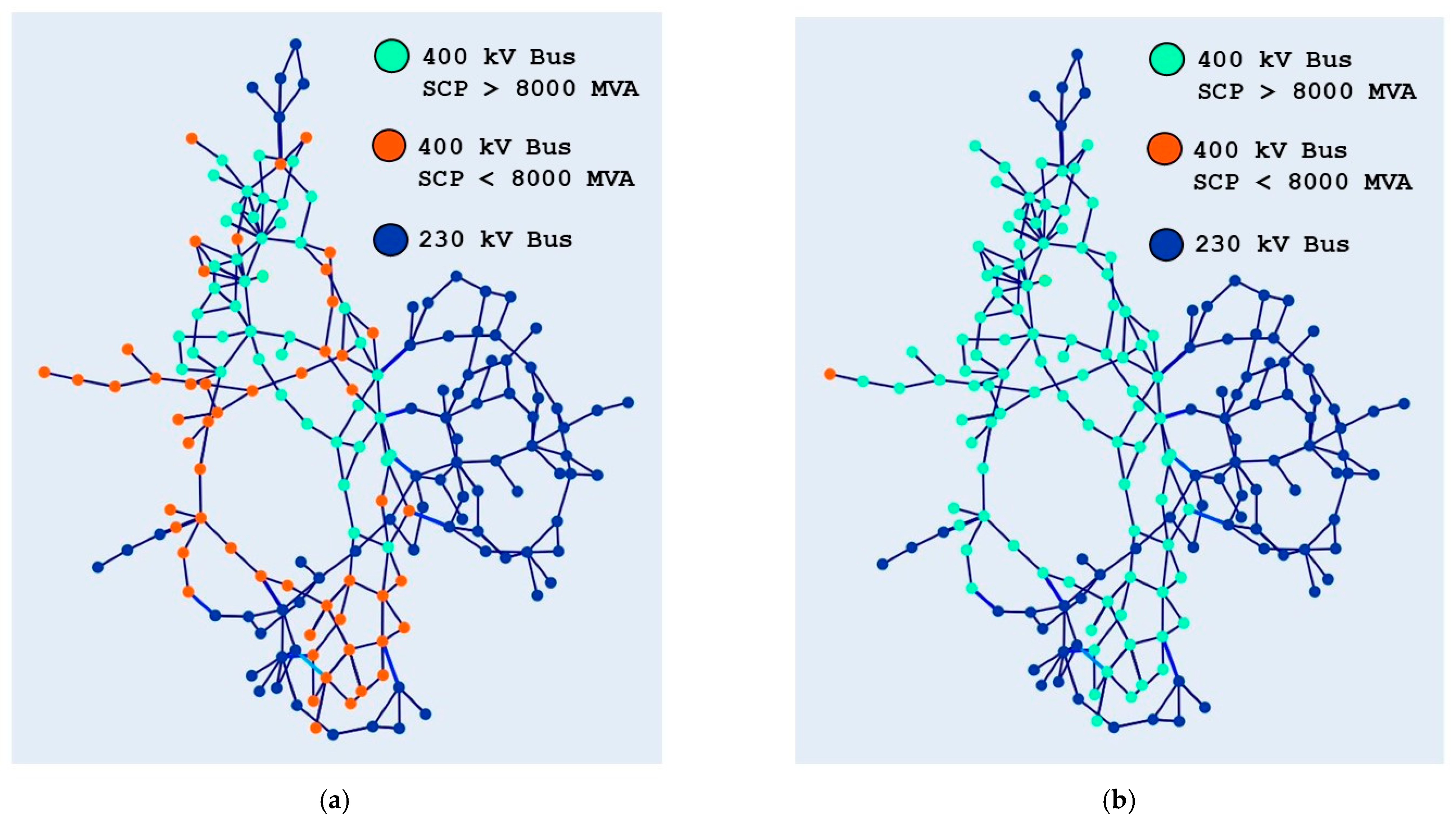
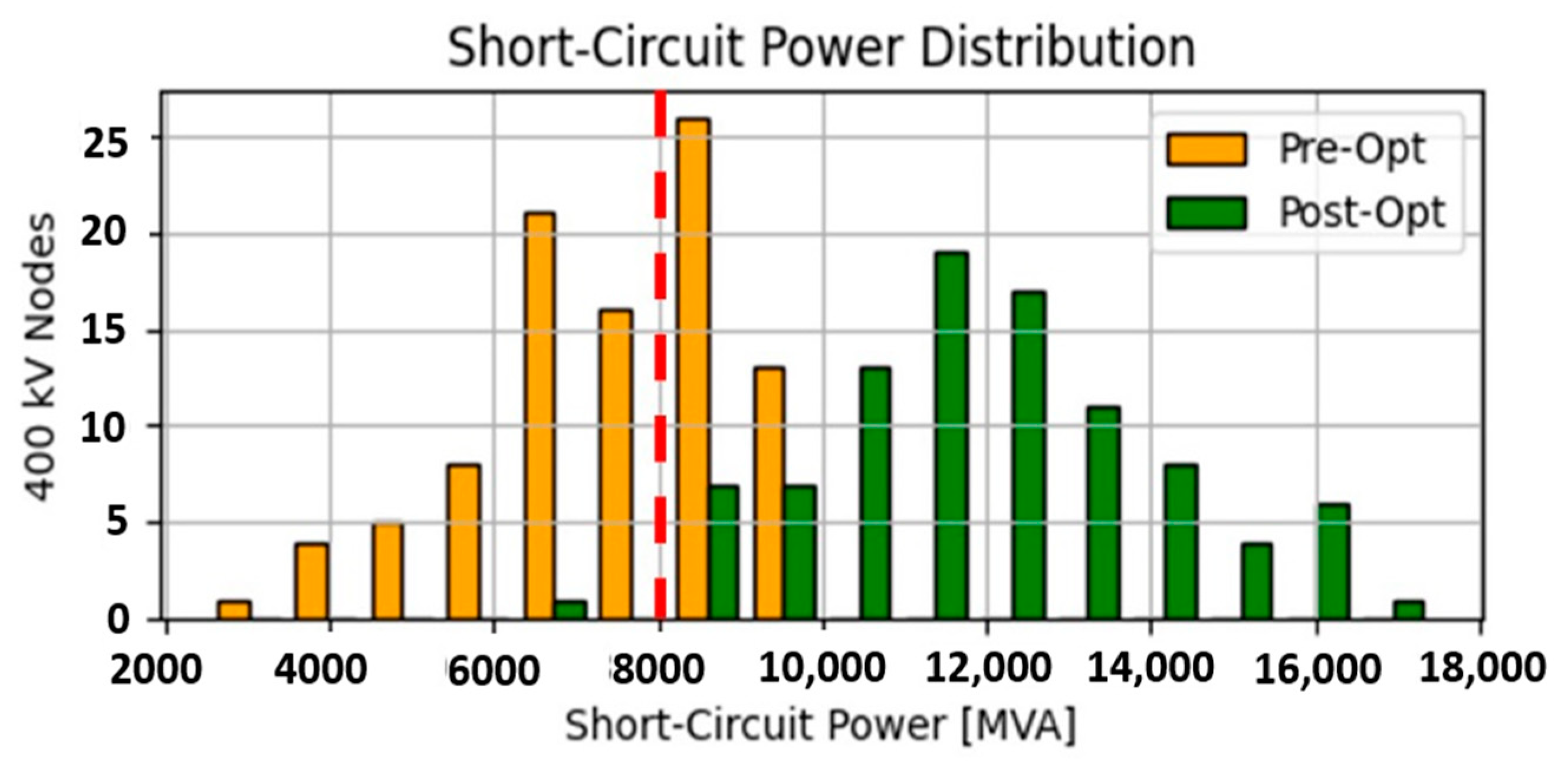
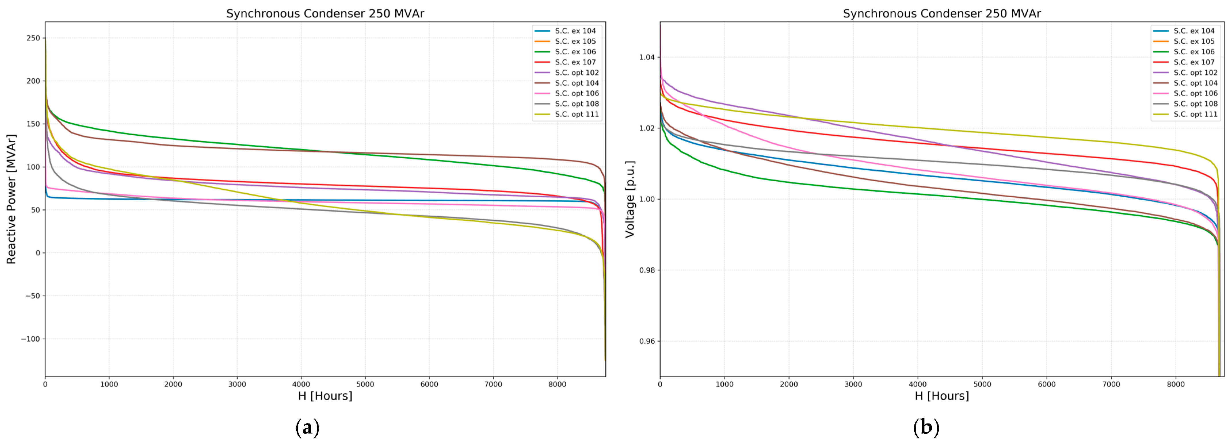
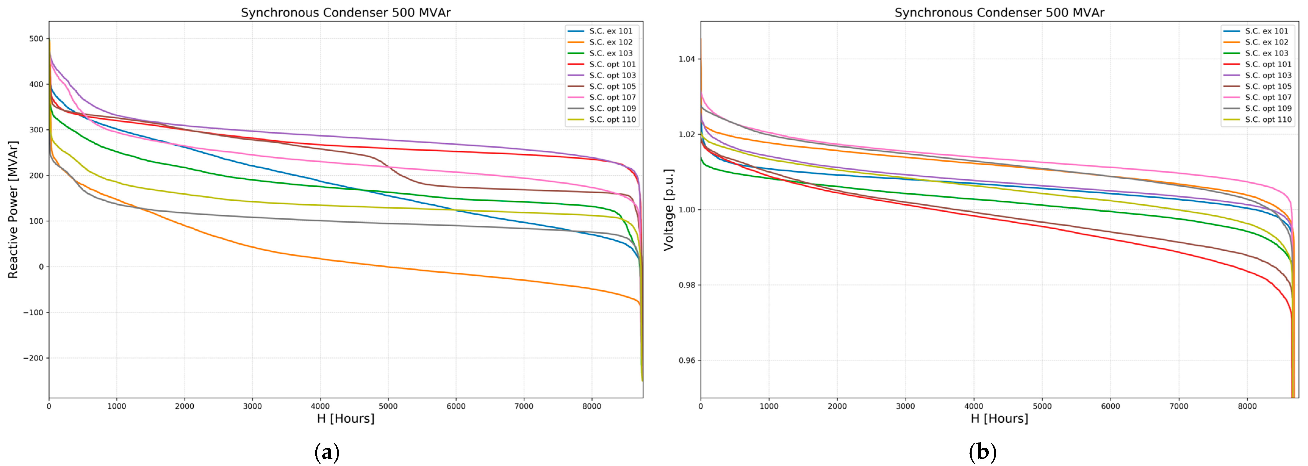
4.2. Sizing and Optimization of the Reactive Compensation
5. Conclusions
Author Contributions
Funding
Data Availability Statement
Conflicts of Interest
References
- IEA. Renewables 2023—Analysis. Available online: https://www.iea.org/reports/renewables-2023 (accessed on 9 January 2025).
- European Commission. ‘Fit for 55’: Delivering the EU’s 2030 Climate Target on the Way to Climate Neutrality. 2021. Available online: https://eur-lex.europa.eu/legal-content/EN/TXT/PDF/?uri=CELEX:52021DC0550 (accessed on 9 January 2025).
- European Commission. Clean Energy for All Europeans, Directorate-General for Energy, Publications Office. 2019. Available online: https://data.europa.eu/doi/10.2833/9937 (accessed on 9 January 2025).
- Terna S.p.A. Scenario Description Document 2024. Available online: https://download.terna.it/terna/Documento_Descrizione_Scenari_2024_8dce2430d44d101.pdf (accessed on 9 January 2025).
- Carlini, E.M.; Gadaleta, C.; Migliori, M.; Conserva, A.; Monno, D.; Moroni, S. Integration of Wind Offshore Generation into the Italian Transmission Network: Connection Solutions and Case Study. In Proceedings of the 2022 AEIT International Annual Conference (AEIT), Rome, Italy, 3–5 October 2022; pp. 1–6. [Google Scholar]
- Hallgren, C.; Arnqvist, J.; Ivanell, S.; Körnich, H.; Vakkari, V.; Sahlée, E. Looking for an Offshore Low-Level Jet Champion among Recent Reanalyses: A Tight Race over the Baltic Sea. Energies 2020, 13, 3670. [Google Scholar] [CrossRef]
- Swider, D.J.; Beurskens, L.; Davidson, S.; Twidell, J.; Pyrko, J.; Prüggler, W.; Auer, H.; Vertin, K.; Skema, R. Conditions and costs for renewables electricity grid connection: Examples in Europe. Renew. Energy 2008, 33, 1832–1842. [Google Scholar] [CrossRef]
- Carlini, E.M.; Moroni, S.; Zagnoni, A.; Gadaleta, C.; De Cesare, A.; Giordano, C.; Migliori, M. Guidelines for the connection and integration of offshore wind energy into the national transmission network. L’Energia Elettr. 2023, 2, 3–16. [Google Scholar]
- Carlini, E.M.; Gadaleta, C.; Migliori, M.; Longobardi, F.; Tulli, M.; Derviskadic, A.; Monge, M.; Persico, A. Challenges and opportunities for Multi-purpose Interconnectors and wind offshore generation. In Proceedings of the 4th SEERC Conference, Trento, Italy, 25–27 September 2024. [Google Scholar]
- Chomać-Pierzecka, E. Offshore Energy Development in Poland—Social and Economic Dimensions. Energies 2024, 17, 2068. [Google Scholar] [CrossRef]
- Offshore Wind Energy. SHP in Europe and in the World in Numbers, Polish Service. Available online: https://www.gov.pl/web/morska-energetyka-wiatrowa/mew-w-europie-i-na-swiecie-w-liczbach (accessed on 14 May 2023).
- Terna S.p.A. Econnextion: Map of Renewable Connections. Available online: https://www.terna.it/it/sistema-elettrico/rete/econnextion (accessed on 9 January 2025).
- Terna S.p.A. Annex A.24 to the Network Code: Identification of Relevant Network Zones; Terna Group: Rome, Italy, 2021. [Google Scholar]
- Italian Regulatory Authority for Energy, Networks and Environment. Decision 19 March 2019. /2019/R/EEL. In Italian. Available online: https://www.arera.it/allegati/docs/19/103-19.pdf (accessed on 9 January 2025).
- Michi, L.; Carlini, E.M.; Migliori, M.; Palone, F.; Lauria, S. Uprating studies for a 230 kV-50 Hz Overhead Line. In Proceedings of the 2019 IEEE Milan PowerTech, Milan, Italy, 23–27 June 2019. [Google Scholar]
- Carlini, E.M.; De Cesare, A.; Gadaleta, C.; Giordano, C.; Migliori, M.; Forte, G. Assessment of Renewable Acceptance by Electric Network Development Exploiting Operation Islands. Energies 2022, 15, 5564. [Google Scholar] [CrossRef]
- Elliott, D.; Bell, K.R.; Finney, S.J.; Adapa, R.; Brozio, C.; Yu, J.; Hussain, K. A Comparison of AC and HVDC Options for the Connection of Offshore Wind Generation in Great Britain. IEEE Trans. Power Deliv. 2016, 31, 798–809. [Google Scholar] [CrossRef]
- Ali, S.W.; Sadiq, M.; Terriche, Y.; Naqvi, S.A.R.; Hoang, L.Q.N.; Mutarraf, M.U.; Hassan, M.A.; Yang, G.; Su, C.-L.; Guerrero, J.M. Offshore Wind Farm-Grid Integration: A Review on Infrastructure, Challenges, and Grid Solutions. IEEE Access 2021, 9, 102811–102827. [Google Scholar] [CrossRef]
- Zhichu, C.; Koondhar, M.A.; Kaloi, G.S.; Yousaf, M.Z.; Ali, A.; Alaas, Z.M.; Bouallegue, B.; Ahmed, A.M.; Elshrief, Y.A. Offshore wind farms interfacing using HVAC-HVDC schemes: A review. Comput. Electr. Eng. 2024, 120 Part B, 109797. [Google Scholar] [CrossRef]
- Dakic, J.; Cheah-Mane, M.; Gomis-Bellmunt, O.; Prieto-Araujo, E. Low frequency AC transmission systems for offshore wind power plants: Design, optimization and comparison to high voltage AC and high voltage DC. Int. J. Electr. Power Energy Syst. 2021, 133, 107273. [Google Scholar] [CrossRef]
- Xiang, X.; Fan, S.; Gu, Y.; Ming, W.; Wu, J.; Li, W.; He, X.; Green, T.C. Comparison of cost-effective distances for LFAC with HVAC and HVDC in their connections for offshore and remote onshore wind energy. CSEE J. Power Energy Syst. 2021, 7, 954–975. [Google Scholar] [CrossRef]
- Van Hertem, D.; Ghandhari, M. Multi-terminal VSC HVDC for the European supergrid: Obstacles. Renew. Sustain. Energy Rev. 2010, 14, 3156–3163. [Google Scholar] [CrossRef]
- Wang, M.; An, T.; Ergun, H.; Lan, Y.; Andersen, B.; Szechtman, M.; Leterme, W.; Beerten, J.; Van Hertem, D. Review and outlook of HVDC grids as backbone of transmission system. CSEE J. Power Energy Syst. 2021, 7, 797–810. [Google Scholar] [CrossRef]
- Hjerrild, J.; Sahukari, S.; Juamperez, M.; Kocewiak, Ł.H.; Vilhelmsen, M.A.; Okholm, J.; Zouraraki, M.; Kvarts, T. Hornsea Projects One and Two–Design and Execution of the Grid Connection for the World’s Largest Offshore Wind Farms. In Proceedings of the Cigre Symposium, Aalborg, Denmark, 4–7 June 2019. [Google Scholar]
- Lauria, S.; Schembari, M.; Palone, F.; Maccioni, M. Very long distance connection of gigawatt-size offshore wind farms: Extra high-voltage AC versus high-voltage DC cost comparison. IET Renew. Power Gener. 2016, 10, 713–720. [Google Scholar] [CrossRef]
- Dakic, J.; Cheah-Mane, M.; Gomis-Bellmunt, O.; Prieto-Araujo, E. HVAC Transmission System for Offshore Wind Power Plants including Mid-Cable Reactive Power Compensation: Optimal Design and Comparison to VSC-HVDC Transmission. IEEE Trans. Power Deliv. 2020, 36, 2814–2824. [Google Scholar] [CrossRef]
- Terna S.p.A. Italian Network Code, Annex A.17. Wind farms: General Connection Rules to HV Networks–Protection, Regulation and Control System. Available online: https://download.terna.it/terna/Allegato%20A.17_8d787c9c8a17ba6.pdf- (accessed on 9 January 2025). (In Italian).
- Implementation of EU Regulation 2016/631 “Requirements for Generators”. Available online: https://download.terna.it/terna/0000/1151/51.pdf (accessed on 9 January 2025). (In Italian).
- Deriu, M.; Migliori, M.; Gadaleta, C.; Cortese, M.; Carlini, E.M.; Dicorato, M.; Forte, G.; Tricarico, G. Grid connection of large offshore wind plants: Techno-economic evaluation of HVAC solutions. In Proceedings of the 2023 AEIT International Annual Conference (AEIT), Rome, Italy, 5–7 October 2023; pp. 1–6. [Google Scholar]
- Terna S.p.A. Grid Development Plan 2023. Available online: https://www.terna.it/it/sistema-elettrico/rete/piano-sviluppo-rete (accessed on 9 January 2025).
- Rehman, A.; Koondhar, M.A.; Ali, Z.; Jamali, M.; El-Sehiemy, R.A. Critical Issues of Optimal Reactive Power Compensation Based on an HVAC Transmission System for an Offshore Wind Farm. Sustainability 2023, 15, 14175. [Google Scholar] [CrossRef]
- Gatta, F.; Geri, A.; Lauria, S.; Maccioni, M. Steady-state operating conditions of very long EHVAC cable lines. Electr. Power Syst. Res. 2011, 81, 1525–1533. [Google Scholar] [CrossRef]
- Ruiz, A.; Rudkevich, A.; Caramanis, M.C.; Goldis, E.; Ntakou, E.; Philbrick, C.R. Reduced MIP formulation for transmission topology control. In Proceedings of the 50th Annual Allerton Conference on Communication, Control, and Computing (Allerton), Monticello, IL, USA, 1–5 October 2012; pp. 1073–1079. [Google Scholar]
- Bak, C.L.; Da Silva, F.F.; CIGRE Working Group. C4.502, Power System Technical Performance Issues Related to the Application of Long HVAC Cables, Technical Brochure 556; CIGRE: Paris, France, 2013. [Google Scholar]
- Deb, K.; Agrawal, S.; Pratap, A.; Meyarivan, T. A fast elitist non-dominated sorting genetic algorithm for multi-objective optimization: NSGA-II. In Parallel Problem Solving from Nature PPSN VI; Lecture Notes in Computer Science (Including Subseries Lecture Notes in Artificial Intelligence and Lecture Notes in Bioinformatics); Springer: Berlin/Heidelberg, Germany, 2000; Volume 1917, pp. 849–858. [Google Scholar] [CrossRef]
- Deb, K.; Pratap, A.; Agrawal, S.; Meyarivan, T. A fast and elitist multiobjective genetic algorithm: NSGA-II. IEEE Trans. Evol. Comput. 2002, 6, 182–197. [Google Scholar] [CrossRef]
- Joint Working Group; CIGRE/CIRED C1.29. Planning Criteria for Future Transmission Networks in the Presence of a Greater Variability of Power Exchange with Distribution Systems; CIGRE/CIRED: Ljubljana, Slovenia, 2017. [Google Scholar]
- Terna S.p.A. Annex A.74 of the Grid Code: Cost-Benefit Analysis Methodology ACB 2.0, Revision 1. February 2019. Available online: https://download.terna.it/terna/0000/1009/13.pdf (accessed on 1 March 2022). (In Italian).
- Terna S.p.A. Scenario Description Document 2022. Available online: https://download.terna.it/terna/Documento_Descrizione_Scenari_2022_8da74044f6ee28d.pdf (accessed on 9 January 2025).
- Hwang, C.L.; Yoon, K. Multiple Attribute Decision Making: Methods and Applications a State-of-the-Art Survey; Springer: Berlin/Heidelberg, Germany, 1981. [Google Scholar]
- Mateo, J.R.S.C. Multi Criteria Analysis in the Renewable Energy Industry; Springer: Berlin/Heidelberg, Germany, 2012; pp. 43–48. [Google Scholar]
- Mazza, A.; Chicco, G. Application of TOPSIS in distribution systems multi-objective optimization. In Proceedings of the 9th World Energy System Conference, Suceava, Romania, 28–30 June 2012; pp. 625–633. [Google Scholar]
- Terna S.p.A. Load Demand: Coverage by Source. 2023. Available online: https://www.terna.it/it/sistema-elettrico/statistiche/evoluzione-mercato-elettrico/domanda-copertura-fonte (accessed on 9 January 2025).
- Available online: https://www.renewables.ninja/ (accessed on 9 January 2025).
- NASA. Modern-Era Retrospective analysis for Research and Applications, Version 2. Available online: https://gmao.gsfc.nasa.gov/reanalysis/MERRA-2/docs/ (accessed on 9 January 2025).
- Löfberg, J. YALMIP: A toolbox for modeling and optimization in MATLAB. In Proceedings of the 2004 IEEE International Conference on Robotics and Automation (CACSD 2004), Taipei, Taiwan, 2–4 September 2004; pp. 284–289. [Google Scholar]


| Sets | Description |
| K | Set of AC branches |
| KDC | Set of DC branches |
| KS | Set of branches of the offshore network, all switchable |
| NB | Set of buses |
| NOWF | Set of buses of the offshore network |
| NSTO | Set of buses with a storage system installed |
| S | Set of scenarios |
| Parameters | Description |
| PTDFS | |K| × |NB| PTDF matrix in scenario s |
| Φs | |K| × |K| Φ matrix in scenario s |
| DCDFS | |K| × |KDC| DCDF matrix in scenario s |
| I | |KS|×|KS| identity matrix, independent of scenario s |
| P0 | |NB\NOWF| vector of nodal power injections of onshore buses at t = Tdim (P0(i) > 0 if power is generated), independent of scenario s |
| POWF | |NOWF| vector of generated power in offshore buses at t = Tdim, independent of scenario s |
| PSTO | |NSTO| vector of rated power of storage systems installed in the onshore network, independent of scenario s |
| FMAX | |K| vector of AC branch capacities, independent of scenario s |
| FMAXDC | |KDC| vector of DC branch capacities, independent of scenario s |
| EOWF | Aggregate power generated at offshore buses at t = Tdim |
| CurtMAX | Maximum allowed curtailment of offshore wind farms, in p.u. of EOWF |
| M | Large enough number |
| Linear Variables | Description |
| PNOD | |NB| × |S| matrix of bus injected powers in each scenario s |
| vT | |KS| × |S| matrix of “flow-canceling transactions” |
| PDC | |KDC| × |S| matrix of power flows through HVDC branches |
| Binary Variables | Description |
| z | |KS| × |S| matrix referred to switchable line status: z(i,s) = 0 if branch i is switched off in scenario s, z(i,s) = 1 if branch i is connected in scenario s |
| Cable Type | S (mm2) | z’ (Ω/km) | c’ (nF/km) | Iz (A) | Pc (MVA) | Sz (MVA) |
|---|---|---|---|---|---|---|
| Single core | 2000 Cu | 0.023 + j0.100 | 240 | 1660 | 4395 | 1150 |
| Three-core | 1600 Cu | 0.019 + j0.120 | 200 | 1070 | 3660 | 740 |
| RES Technology | [GW] |
|---|---|
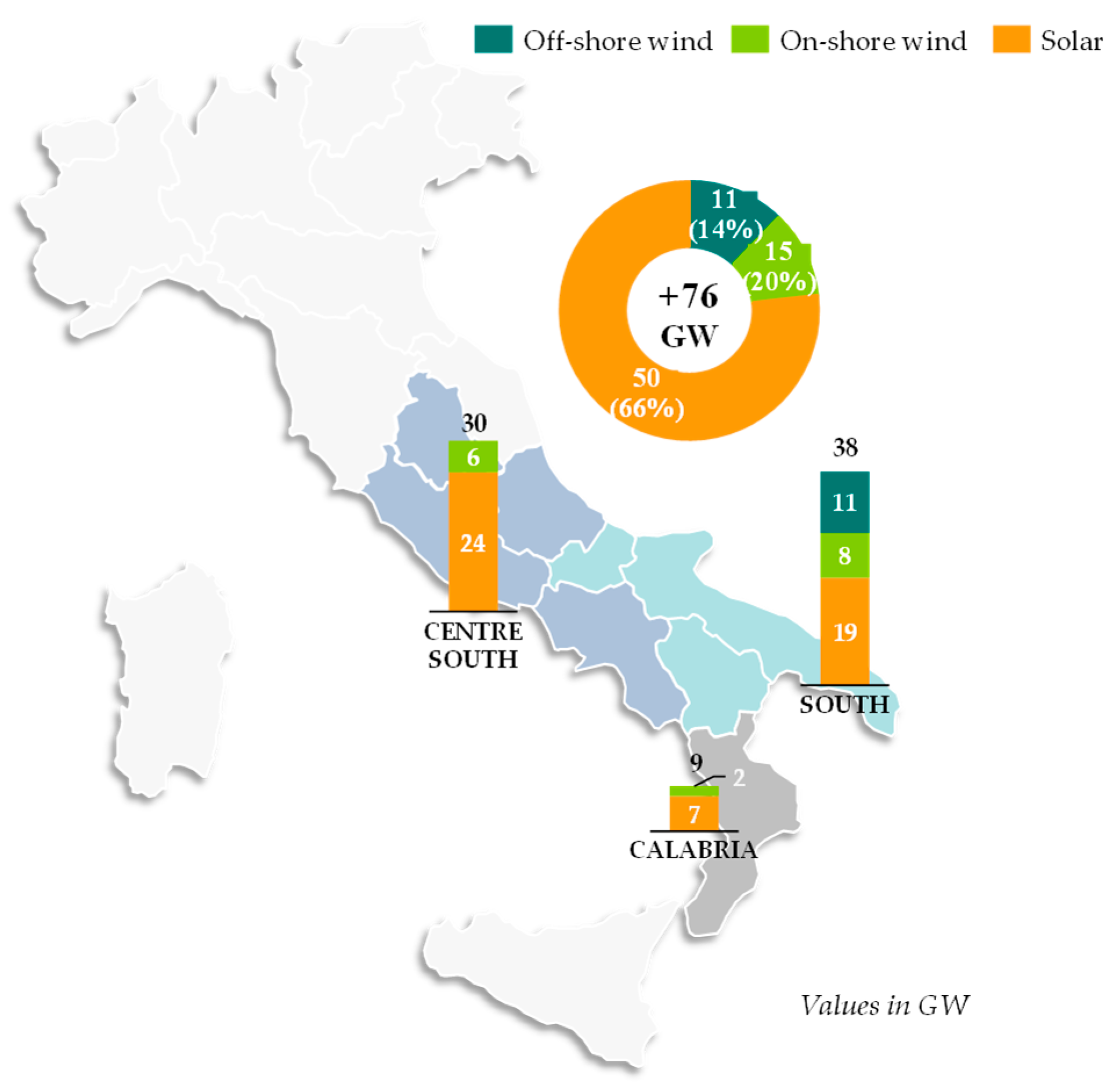
| Solar photovoltaic | 50 |
| Onshore wind | 15 |
| Offshore wind | 11 |
| Storage capacity | [GWh] |
| 91.2 | |
| Load | [TWh] |
| 110 |
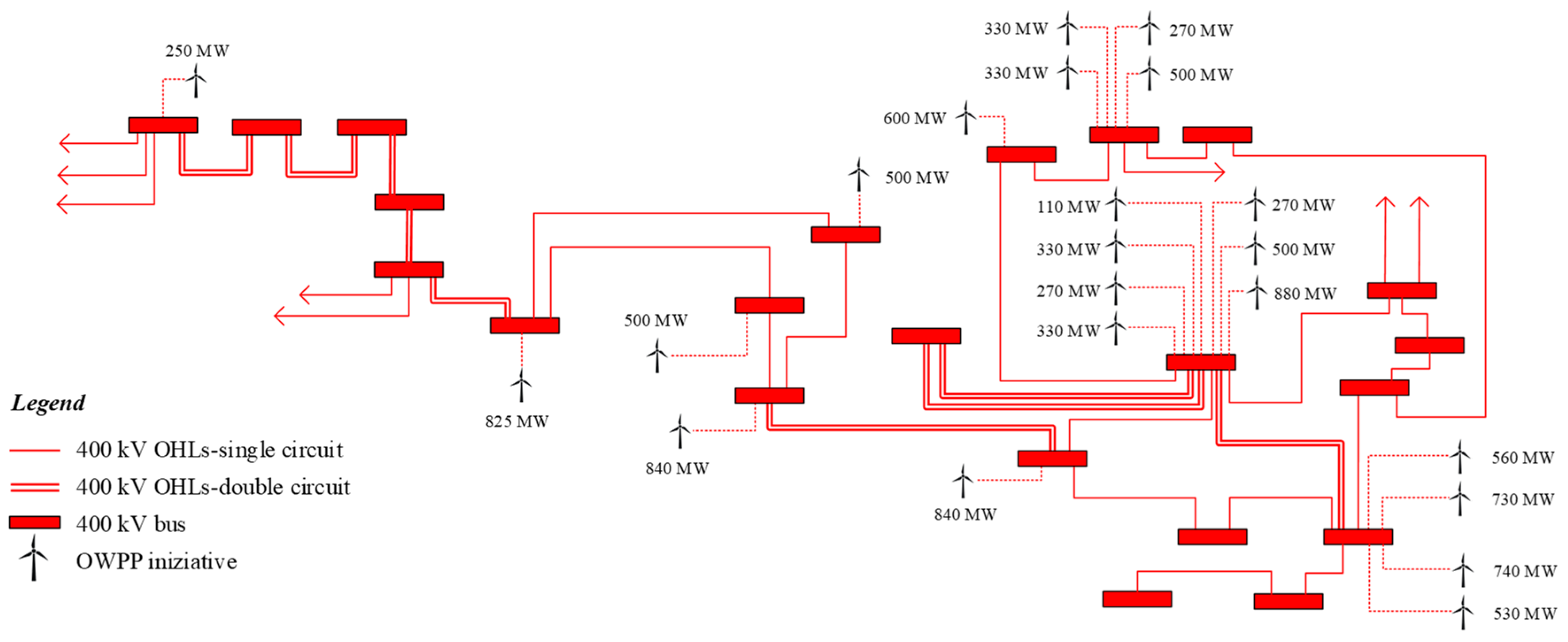
| Bus | Number of OWFs | Capacity (MW) |
|---|---|---|
| 1 | 5 | 1300 |
| 2 | 4 | 1330 |
| 3 | 1 | 250 |
| 4 | 4 | 2570 |
| 5 | 1 | 840 |
| 6 | 2 | 1300 |
| 7 | 3 | 1980 |
| 8 | 2 | 1350 |
| Operating Condition | Pgen (MW) | Curtailment (%) | |
|---|---|---|---|
| Winter scenario | N security | 8300 | 22.7 |
| N − 1 security | 8300 | 22.7 | |
| Summer scenario | N security | 7700 | 28.3 |
| N − 1 security | 7460 | 30.6 | |
| Operating Condition | Bus 1 | Bus 2 | Bus 3 | Bus 4 | Bus 5 | Bus 6 | Bus 7 | Bus 8 | |
|---|---|---|---|---|---|---|---|---|---|
| Winter scenario | N security | 0 | 26.8 | 0 | 7.3 | 100 | 15.9 | 0 | 66.4 |
| N − 1 security | 0 | 26.8 | 0 | 7.3 | 100 | 15.9 | 0 | 66.4 | |
| Summer scenario | N security | 0 | 23.4 | 77.4 | 0 | 0 | 44.9 | 47.6 | 79.9 |
| N − 1 security | 0 | 23.7 | 100 | 0 | 11.6 | 33.8 | 46 | 100 | |
| Operating Condition | Pgen (MW) | Curtailment (%) | |
|---|---|---|---|
| Winter scenario | N security | 4930 | 54.1 |
| N − 1 security | 4890 | 54.5 | |
| Summer scenario | N security | 4000 | 62.3 |
| N − 1 security | 3560 | 66.8 | |
| Operating Condition | Bus 1 | Bus 2 | Bus 3 | Bus 4 | Bus 5 | Bus 6 | Bus 7 | Bus 8 | |
|---|---|---|---|---|---|---|---|---|---|
| Winter scenario | N security | 11.0 | 0 | 100 | 100 | 100 | 88.2 | 0 | 71.1 |
| N − 1 security | 47.8 | 0 | 100 | 100 | 100 | 26.1 | 0 | 100 | |
| Summer scenario | N security | 37.9 | 0 | 100 | 100 | 100 | 100 | 0 | 100 |
| N − 1 security | 100 | 0 | 100 | 20.0 | 100 | 83.6 | 100 | 100 | |
Disclaimer/Publisher’s Note: The statements, opinions and data contained in all publications are solely those of the individual author(s) and contributor(s) and not of MDPI and/or the editor(s). MDPI and/or the editor(s) disclaim responsibility for any injury to people or property resulting from any ideas, methods, instructions or products referred to in the content. |
© 2025 by the authors. Licensee MDPI, Basel, Switzerland. This article is an open access article distributed under the terms and conditions of the Creative Commons Attribution (CC BY) license (https://creativecommons.org/licenses/by/4.0/).
Share and Cite
Carlini, E.M.; Gadaleta, C.; Migliori, M.; Longobardi, F.; Luongo, G.; Lauria, S.; Maccioni, M.; Dell’Olmo, J. Offshore Network Development to Foster the Energy Transition. Energies 2025, 18, 386. https://doi.org/10.3390/en18020386
Carlini EM, Gadaleta C, Migliori M, Longobardi F, Luongo G, Lauria S, Maccioni M, Dell’Olmo J. Offshore Network Development to Foster the Energy Transition. Energies. 2025; 18(2):386. https://doi.org/10.3390/en18020386
Chicago/Turabian StyleCarlini, Enrico Maria, Corrado Gadaleta, Michela Migliori, Francesca Longobardi, Gianfranco Luongo, Stefano Lauria, Marco Maccioni, and Jacopo Dell’Olmo. 2025. "Offshore Network Development to Foster the Energy Transition" Energies 18, no. 2: 386. https://doi.org/10.3390/en18020386
APA StyleCarlini, E. M., Gadaleta, C., Migliori, M., Longobardi, F., Luongo, G., Lauria, S., Maccioni, M., & Dell’Olmo, J. (2025). Offshore Network Development to Foster the Energy Transition. Energies, 18(2), 386. https://doi.org/10.3390/en18020386