Abstract
This research aims to present a study of the effects of the Tesla transformer in order to find the proper dimensions. We created a design of the Tesla transformer to reduce the high-voltage electric field-stress problem that happens between primary winding and secondary winding. Because the Tesla transformer is used to induce voltage between these two windings through the air, problems with insulation occur. The winding that has space is dielectric; while there is high voltage in a transformer, it causes flashover voltage between the high-voltage winding and low-voltage winding, which damages the transformer and other devices. Research process: Research was conducted to study the laydown model (positioning) of the two windings in the transformer. By considering this, we induced a proper Tesla transformer that was reproduced by using the FEMLAB program. Moreover, we compared the Tesla transformer reproduction, which created a voltage of 120 kV and a frequency of 120 kHz. The result from the comparison is a proper laydown position of the primary winding and voltage, which has been designed without the flashover. The whorl coil has to be wound at a 60-degree angle relative to the floor and can induce more voltage than other models. The voltage and corresponding electric field stress were measured for the primary winding at various angles relative to the floor (0-, 30-, 45-, 60-, and 90-degree angles) to determine the configuration. The results from the reproduction using the FEMLAB program and testing demonstrated that no flashover occurred between the high-voltage winding to the low-voltage winding when the primary winding was positioned at a 60-degree angle.
1. Introduction
In the manufacturing of porcelain insulators, high-voltage transformers are used to distribute voltage during the testing phase to ensure the primary quality of the insulators and verify that they are not defective. This is done by causing flashover on the surface of the insulators, which follows the standard ANSI C.29.1-2018 [1], and using high frequencies to test for defects inside. It would affect the high electric field stress that occurs between the primary coil and secondary coil (Lp, Ls) because this type of transformer is an air-axis transformer. This would pose a problem in the insulator coil with electric air, creating a flashover between the two sets of coils. Maintaining a suitable distance from the coil would reduce this problem. To reduce the problem, the voltage should not exceed the determined amount set by the high-voltage, high-frequency transformer. The advantage of air-core transformers is that there is no magnetic saturation, making them suitable for high-frequency applications [2]. Thus, this research is aimed at studying the effect of high-voltage, high-frequency transformer (Tesla transformer) induction. To find the suitable dimension by analyzing the results obtained in this research, we used the model circuit of the Tesla transformer by using the FEMLAB program and compared these with the testing results received from the built-up Tesla transformer [3].
The coil of Tesla was invented by Nikola Tesla in 1891 [4,5]. The resonance between the sides of the secondary coils on the transformer is the operating principle of the Tesla coil [5,6]. The transformer of Tesla is a device that provides high electrical potential. The Tesla coil, also known as a resonant transformer, refers to a transformer that operates at a specific resonant frequency rather than at all frequencies. The coil or winding that generates electrical sparks is the secondary coil, which is constructed from an inductor, a capacitor, and a resistor connected, as shown in Figure 1.
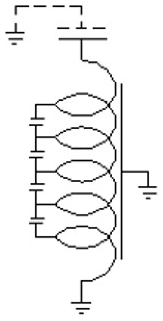
Figure 1.
Coil made from inductors, capacitors, and resistors.
Voltage is generated from damped oscillations at a frequency of 50 to 400 kilohertz. The Tesla transformer was created to effectively test the electrical conditions of suspensions and post-type insulators [7,8]. A Tesla coil is an oscillator tuned with a capacitor that drives an air-core resonant transformer to generate a high voltage at a low current. The high-voltage transformer increases the voltage to a level sufficient to jump across the spark gap, which acts as a switch in the primary circuit, thereby producing high voltage in the secondary circuit [9,10,11]. The high-voltage pulses generated will have an amplitude of several megavolts and can discharge electricity over several meters [12,13]. An electric field is a quantity that represents the region where an electric charge exerts a force on other charged particles within its vicinity. The unit of an electric field is either newton per coulomb (N/C) or volt per meter (V/m), which are equivalent. The electric field consists of photons and stores electrical energy, with the energy density being proportional to the square of the field strength [14].
In 2008, the electric field and components were optimally designed using the FEMLAB software (Version 6.0). The IEC standard was used to determine the PD value in the design of the cable terminator and to design the cable connector with SF6 insulation. The electrical stress was analyzed [15]. In 2010, a cost-effective high-performance transformer of Tesla was constructed and designed to test an insulator. The transformer output was designed at 500 kV. This article presents the results of the experimental simulations from the transformer of Tesla to suit the main design parameters [16]. In 2023, studies were conducted on high-frequency transformers integrated into solid-state transformers, in particular, developing procedures that allow for the most suitable design of high- frequency transformers, as well as the effects of transformer operation at high frequencies and the associated solutions that minimize their effects. This paper demonstrates a systematic procedure for designing HFTs according to the desired requirements of each project [17].
Therefore, this paper analyzed the electric field distribution on primary windings of high-voltage, high-frequency transformers with variable characteristics.
The objectives of this paper are as follows:
- -
- Analyze the electricity field distribution at low voltages and the angles 0, 30, 45, 60, and 90 degrees.
- -
- Compare the voltage flow out of the putting primary coil.
- -
- Compare the external frequency of the primary coil putting.
- -
- Compare the results of the distribution electricity field model between the primary coil (Lp) and secondary coil.
2. Finite Element Method
The finite element method consists of six major steps as follows:
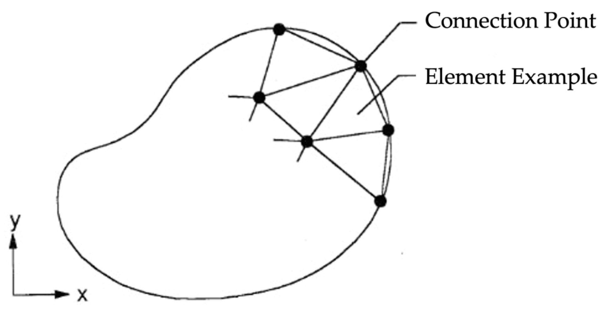
Step 1: Divide the boundary shape of the problem into smaller elements, as shown in Figure 2. These boundaries can pertain to various types of problems, such as deformation and stress in solids, heat transfer in solids or fluids, or fluid flow problems.

Figure 2.
Breaking down the shape of the problem into elements of different sizes.
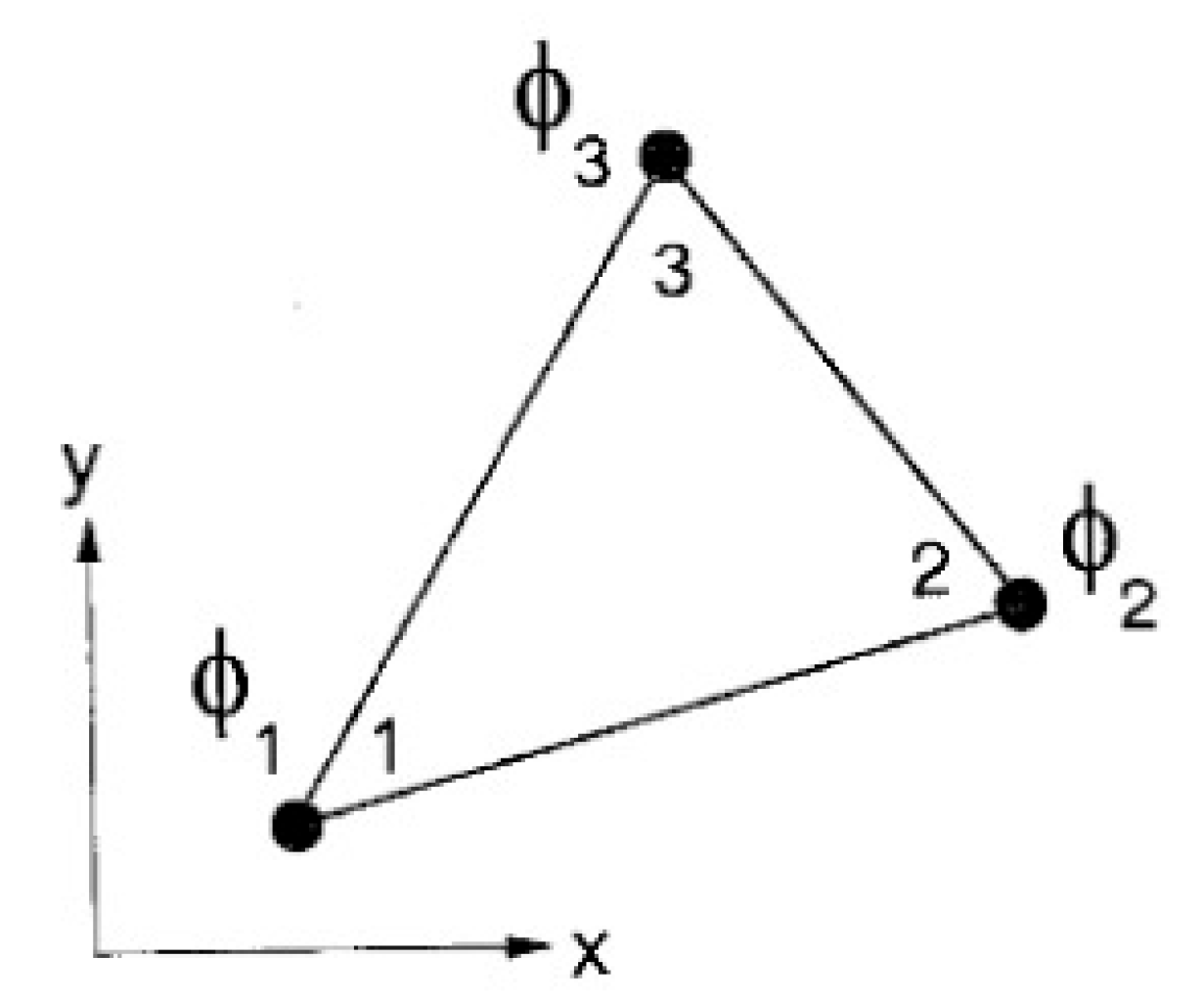
Step 2: Select the interpolation functions within the element (element interpolation functions). For example, consider a triangular element in two dimensions (as shown in Figure 3). This element consists of three nodes numbered 1, 2, and 3, as illustrated in Figure 3.

Figure 3.
A triangular element consisting of three points with an unknown at the position of the connection point.
At these nodes, the unknown values (nodal unknowns) are represented as ϕ1, ϕ3, and ϕ3. These unknowns at the nodes may represent deformation magnitudes if solving a deformation problem in solids, temperature values if solving a heat transfer problem, fluid velocity values if solving a fluid flow problem, and so on. The distribution of these unknown values across the element can be expressed in terms of the interpolation functions and the nodal unknowns as follows:
With Ni(x,y), i = 1, 2, 3 representing the inner element approximation function, Equation (2) can be written in matrix form as follows.
where represents the row matrix of the approximation function within the elements, and {ϕ} represents the column matrix vector containing the unknowns at the vertices of the elements.
Step 3: Creating element equations. For example, the equations of the triangular elements in Figure 3 are in the following form:
The lower index e indicates that the matrices are element-level matrices. This third step can be considered as the heart of the finite element method. The element equations need to be constructed to correspond to the differential equations of the problem. In the next section, we will see that the element equations can be constructed directly from the differential equations by applying the method of weighted residuals, which is considered a general method that is popularly applied to various problems today.
Step 4: First, combine the equations derived from all the elements to form a larger system of equations, as follows:
Step 5: Apply the boundary conditions to the system of Equation (5) and then solve this system of equations to find the unknowns at the interface, which could be values for displacement due to deformation in a solid, values for temperature for a heat transfer problem, values for fluid velocity for a flow problem, etc.
Step 6: Calculate other continuous values after calculating the values at the junctions from Step 5. For example, after knowing the values of the deformation movement in the solid, the values of stress and strain can be calculated; when the values of the temperatures at various junctions are known, they can be used to calculate the amount of heat transfer; when the flow velocity is known, it can be used to calculate the total flow rate, etc.
From these six steps, it can be seen that the finite element method is a systematic and step-by-step method. The key is to construct the element equations (Step 3) that correspond to the given differential equations of the problem. The other steps are a combination of different kinds of knowledge that we have studied in previous chapters, starting from the knowledge of approximation in the range, which we use to construct the approximation function within the element, as well as the knowledge of numerical integration, which is required to calculate the matrices of some elements and the knowledge of solving the system of equations to find the result at the point of connection.
3. Equipment and Research Model
The equipment used in the research is as follows:
- MATLAB (Version R2024b-acdemic use) Program: Using the Tesla transformer model as a design before building the real one.
- FEMLAB Program: Used as a model to distribute the electricity field in the Tesla transformer.
- PVC tube with a diameter of 10.16 cm: Used as the axis for the Ls secondary coil binding.
- Enamel copper coil size 31 SWG: Used for the LS secondary coil binding.
- Copper tube 0.0762 cm diameter 0.635 cm 1.27 cm: Used for the Lp primary coil and transformer protection ring.
- Motor 1 phase: Speed at 1450 rounds per second to drive the rotary spark cap.
- Low-voltage capacitor polypropylene size of 15 nF and 1600 V.
- Neon sign transformer 230 V/15,000 V: Used for the transformer power distribution of the low-voltage Tesla transformer.
4. Method
- High-voltage circuit model: High-frequency voltage at 120 kV and a high voltage at 120 kHz, using the MATLAB and FEMLAB programs.
- Create the model of components and several structures of high voltage and high frequency.
- Build up the components and several structures of high voltage and high frequency.
- Test to find the best features in the operation of high-voltage, high-frequency systems and correct the defective parts.
- Collect the results from the calculations and the results from the model using the FEMLAB program.
- Conclude the research and testing of the Tesla transformer circuits.
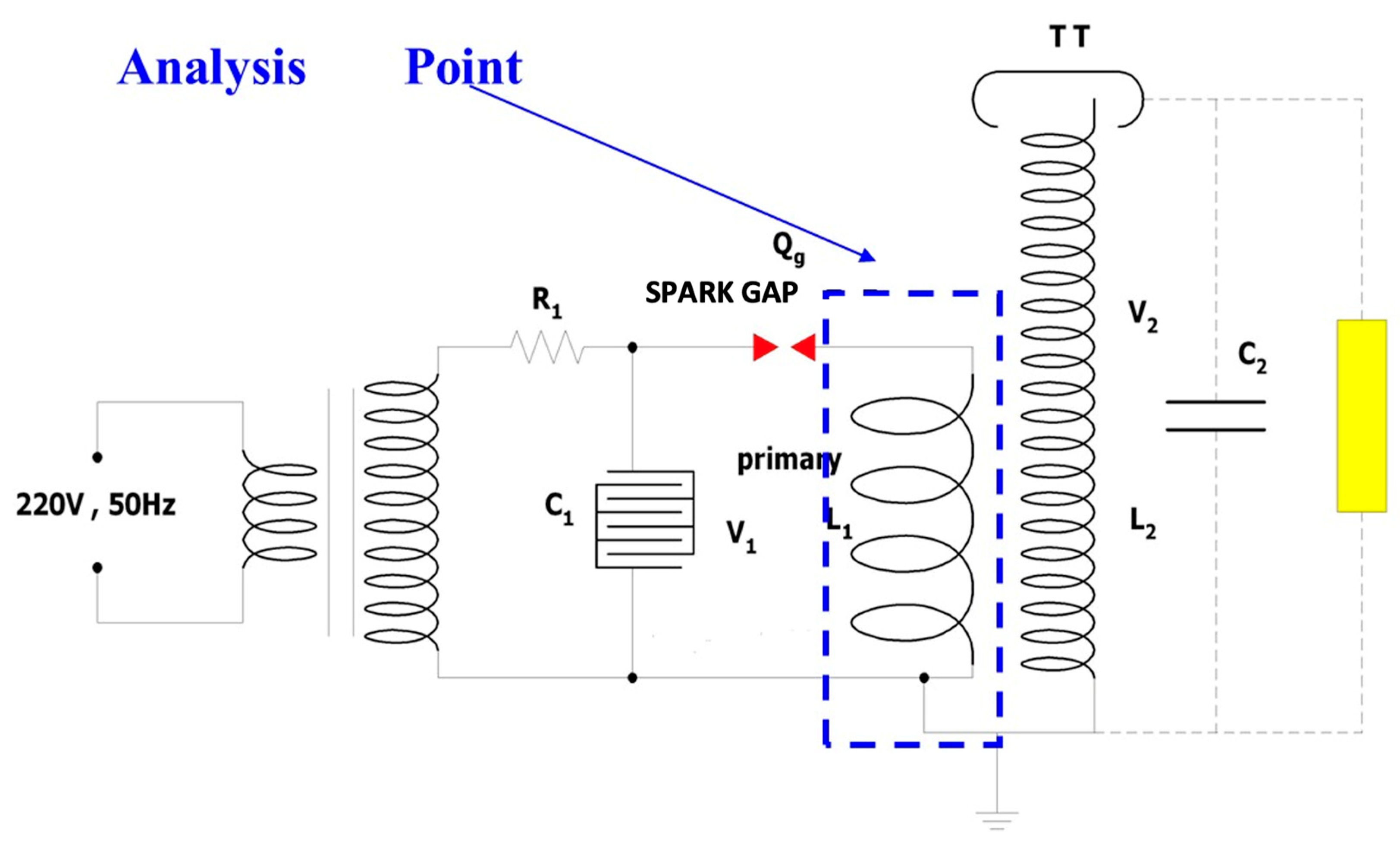
The transformer of the Tesla circuit is shown in Figure 4.
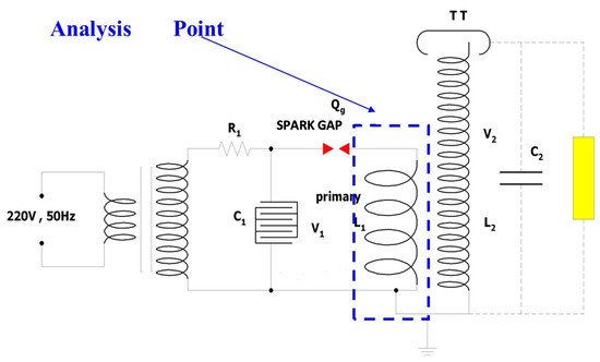
Figure 4.
Transformer of Tesla circuit. C1 is the main capacitor. L1 is the main inductor. C2 is the secondary capacitor. L2 is the secondary inductor. Qg is the spark gap. R1 is resistance. V1 is the voltage at the Primary coil of the Tesla transformer. V2 is the voltage obtained by the induction of the Tesla transformer on the Secondary coil.
The high voltage is 120 kVrms, the frequency is 120 kHz, the voltage impulse is 0–15 kVrms, and the capacity C2 value is around 40 pF, regarding the equation that is used for calculating the parameters [18,19,20]. The Tesla transformer testing result has placed the Lp coil at the angles of 90, 60, 45, 30, and 0 degrees. The oscillation that retains it should be calculated in each type. The Tesla transformer testing result placed the Lp coil at the angles 90, 60, 45, 30, and 0 degrees. The oscillation that retains it should be calculated in each type.
- -
- In the case that oscillation occurs between L1 and C1, the frequency that would occur can be calculated using Equation (6).
- -
- The condition that occurs from oscillation low-voltage induction and high-voltage tuning [21] can be calculated using Equation (7).
- f1 is the primary resonant frequency (Hz).
- L1 is the primary inductance (H).
- C1 is the primary capacitance (F).
Tesla transformers have an output current that is in the form of a high-frequency pulse, so the design must take into account the skin effect of the conductor.
where H is the height of the coil, L is inductance, N is the number of turns, and R is the radial of the coil. The coil capacitance can be calculated using Equation (9).
where Cs is the stray capacitance.
Table 1 shows 45° primary side L1 is 72.09 μH, and C1 is 6.366 μF. The secondary side L2 is 43.97 mH, and C2 is 40 pF.

Table 1.
The tube size and the height suitable for binding high-voltage coil.
Table 2 shows the diameter in centimeters, high/diameter in centimeters, and length of coil binding in centimeters.
Table 2.
The tube diameter and coil binding.
Figure 5 shows R is the diameter radius to the center of the coil (cm). H is the height of the binding (cm).
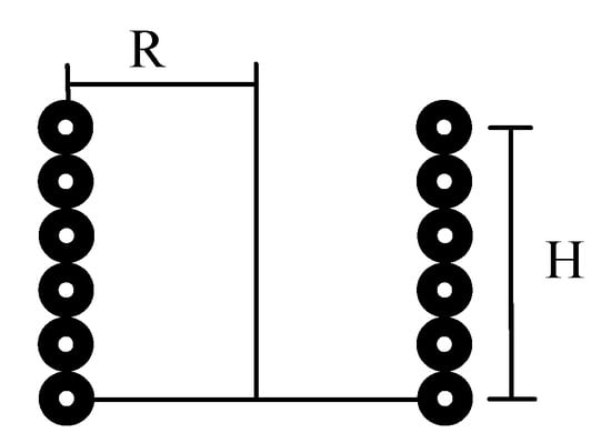
Figure 5.
The dimension for binding high-voltage coil [22,23].
Low-voltage coil model
1. Angle with the floor at 30°, 45°, and 60°, using a copper tube size of 0.79 cm with a thickness of 0.0762 cm for low-voltage coil.
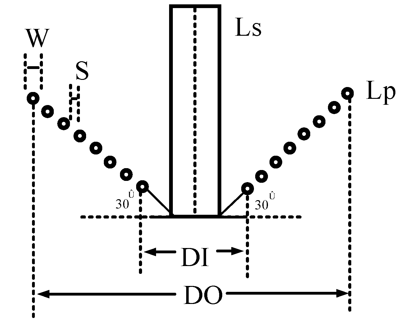
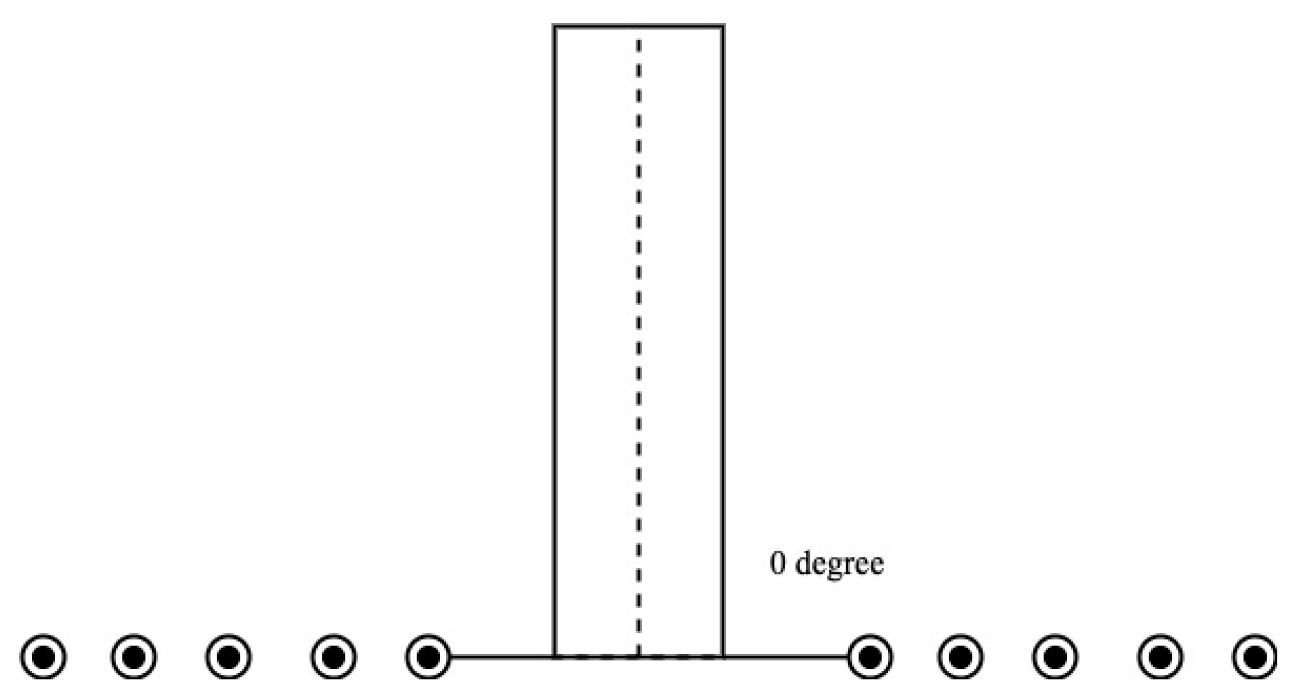
Figure 6 shows Angle to the floor at 0° using a copper tube size of 0.79 cm with a thickness of 0.0762 cm for a low voltage [23]. W is the diameter of the copper tube = 0.79 cm. S is the binding distance = 1.27 cm. DI is the inside diameter of Lp = 35.56 cm. DO is the outside diameter of Lp = 86.36 cm.

Figure 6.
The primary coil at the angles of 30°, 45°, and 60° [24].
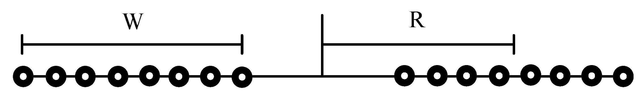
Figure 7 shows W is the width of the total winding. R is the average radius of the total winding.
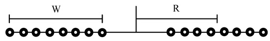
Figure 7.
The primary coil at the angle 0° [23].
5. Results from FEMLAB Electric Field Simulation Process
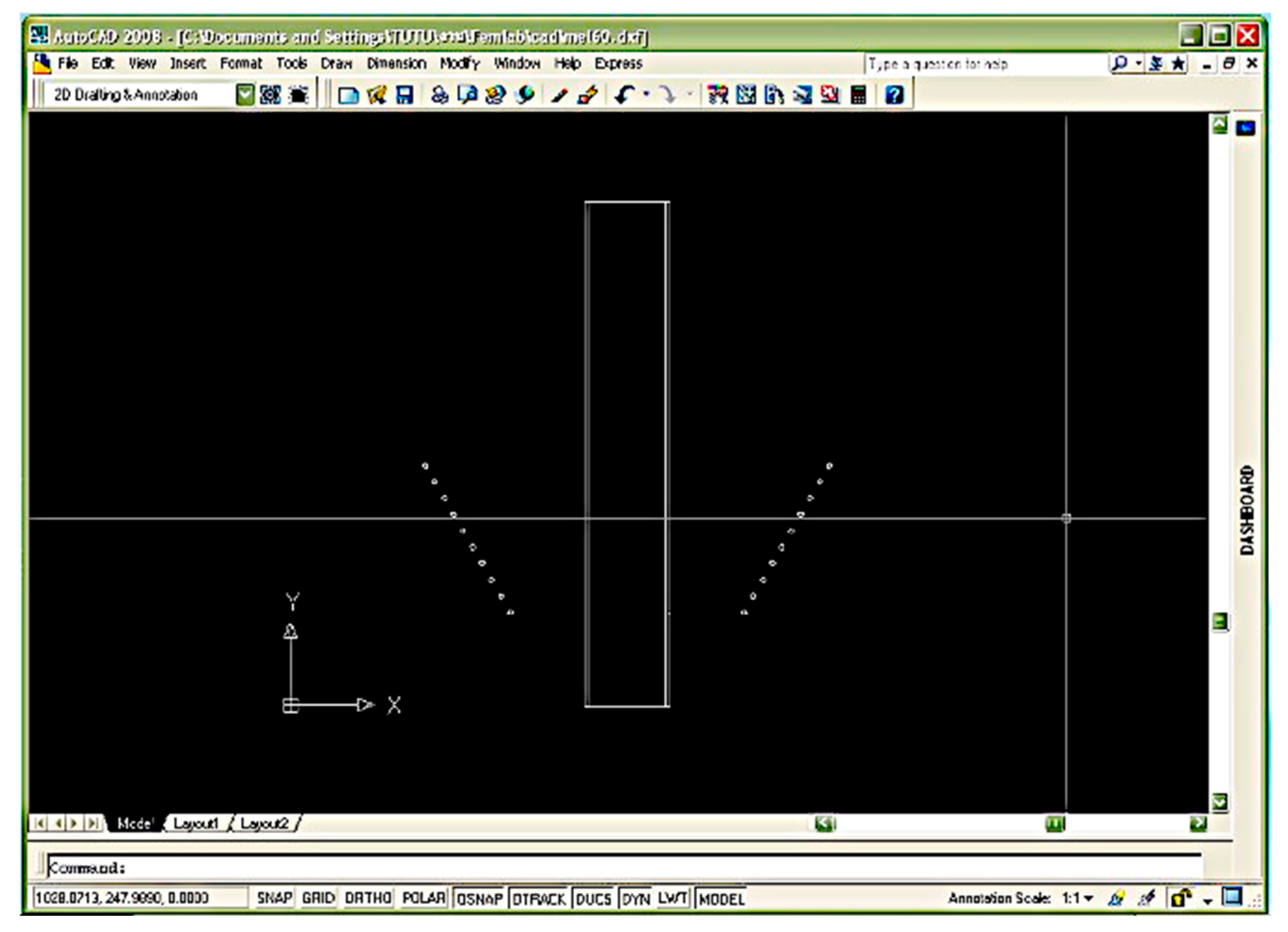
The researcher modeled the coil designs using AutoCAD (Version: Autodesk AutoCAD education) and then imported them into the FEMLAB program to set the parameters before running the simulations.
Figure 8 shows analyze the electric field based on the placement angles of the primary coil at 0, 30, 45, 60, and 90 degrees. This process led to the simulation of the electric field characteristics of the primary voltage coil, as presented in the following section.
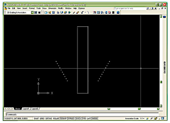
Figure 8.
The primary voltage coil was modeled using AutoCAD to facilitate analysis in the FEMLAB program.
6. Results
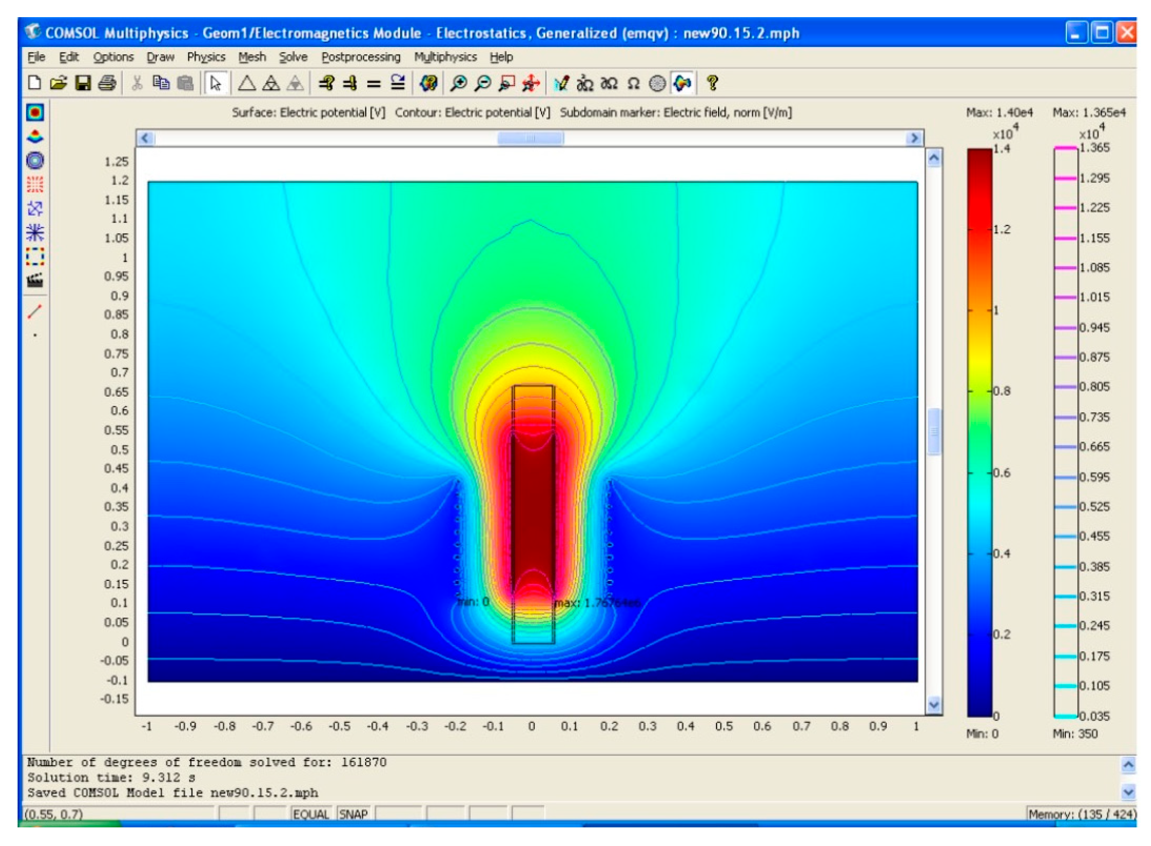
The model of electric field distribution in a high-voltage, high-frequency transformer, following the finite element process, was created using the FEMLAB program. It was determined that the voltage in the low coil should have an electricity voltage of 15 kV. A case study of the hypothesis is based on dimensions of 5 degrees, considering the design of the coils at 0, 30, 45, 60, and 90 degrees. The study examines how much each type affects the electric field in creating the output voltage of the Tesla transformer. Emax demonstrates the results from the FEMLAB analysis. The high-voltage coil has a permittivity tube of a PVC size of 3.5 and with 120 kV of voltage [22,24]. The power supply used is adapted from neon transformers or units with a 220 V input and outputs ranging from 1 kV up to 15 kV in 25/30 mA and 50/60 mA.
The comparison of the electricity field model and the angles of the low-voltage coil are at five degrees viz ninety, sixty, forty-five, thirty, and zero degrees. The results of the model of electricity field distribution at a low voltage are shown in Figure 9, Figure 10, Figure 11, Figure 12, Figure 13 and Figure 14.
Figure 9.
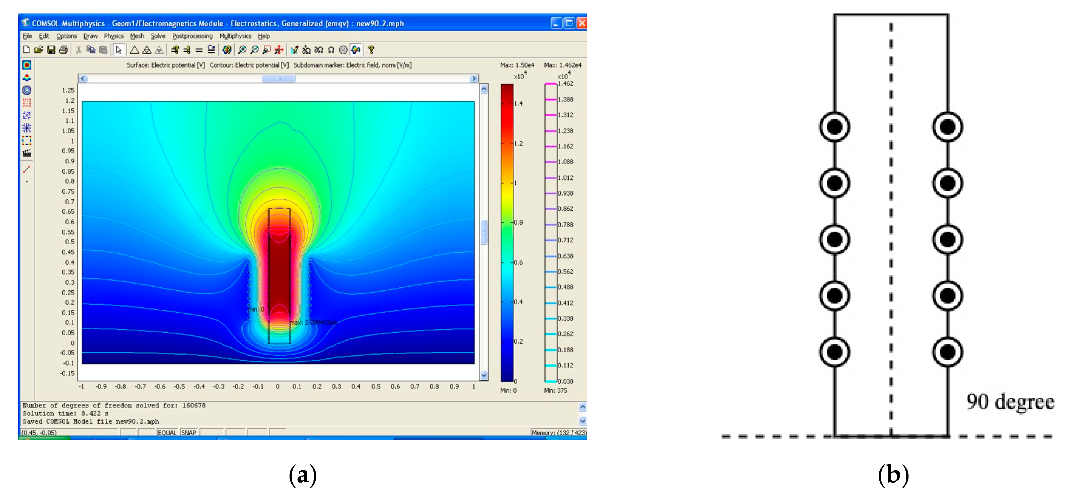
The model of the electricity field at the primary voltage coil at a 90-degree angle: (a) in the case of the FEMLAB program and (b) in the case of the model.
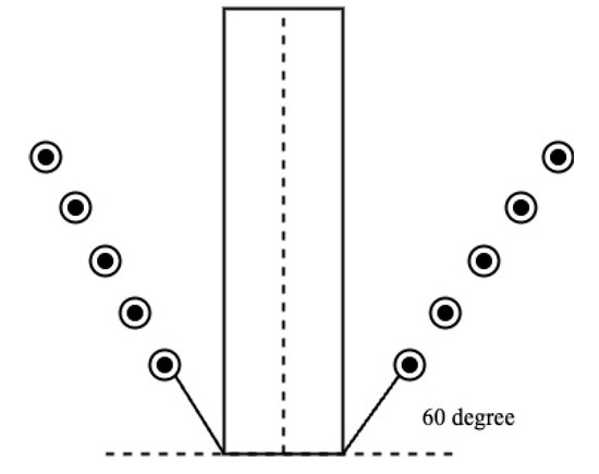
Figure 10.
The model of the electricity field with the low-voltage coil at a 60-degree angle.

Figure 11.
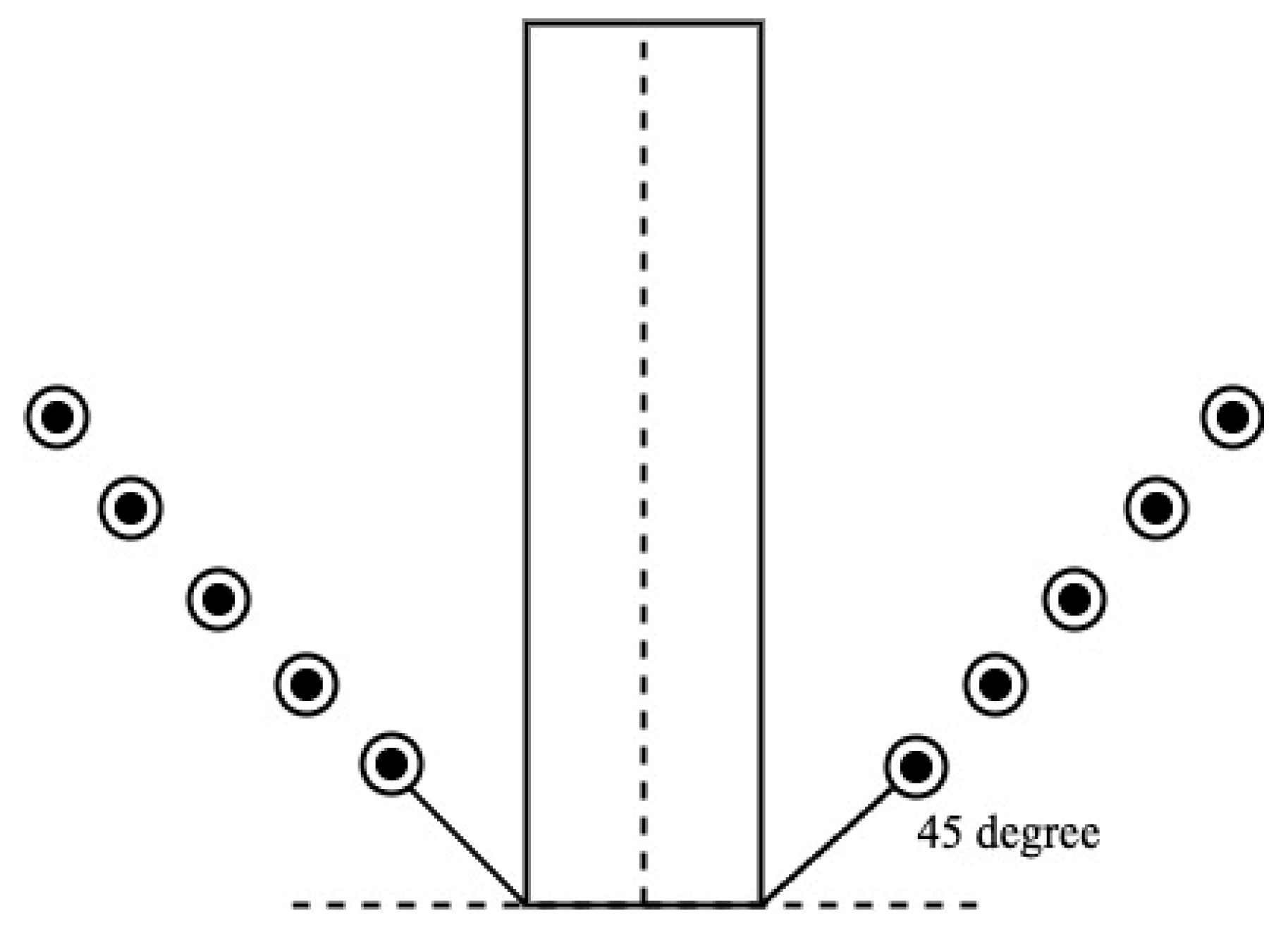
The model of the electricity field with the low-voltage coil at a 45-degree angle.

Figure 12.
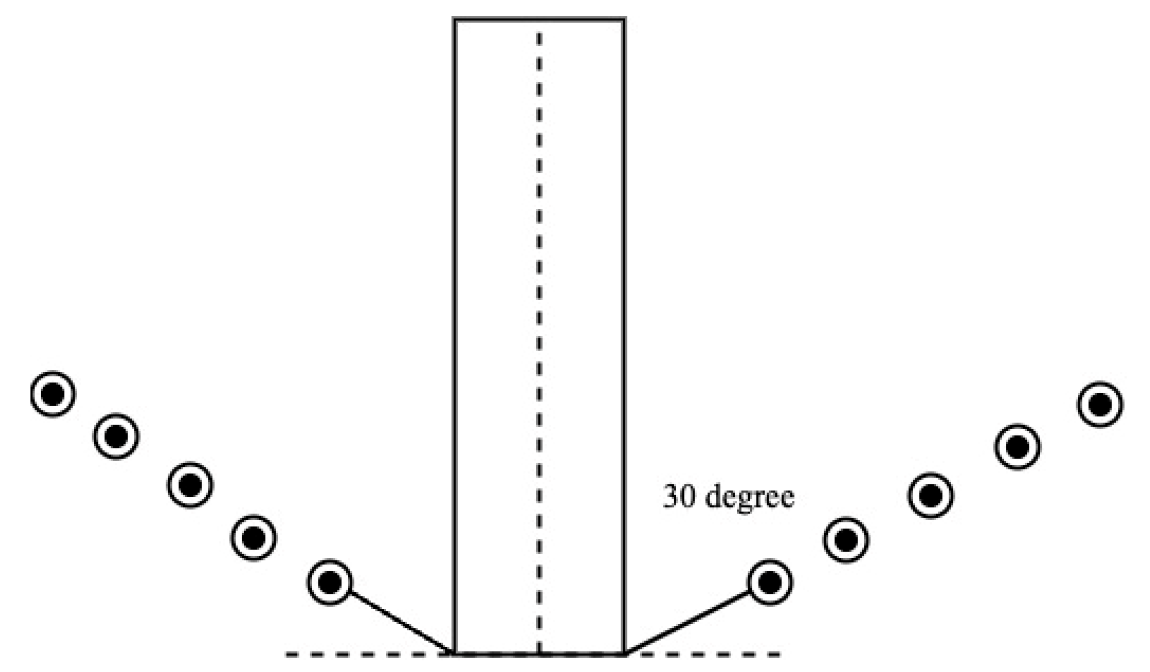
The model of the electricity field with the low-voltage coil at a 30-degree angle.
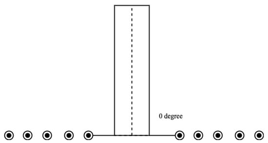
Figure 13.
The model of the electricity field with the low-voltage coil at a 0-degree angle.
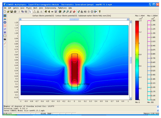
Figure 14.
The model of the electricity field with the low-voltage coil at a 90-degree angle from the floor. It expands the distance between the Lp and Ls coil from the previous 10.16 cm to 13.97 cm, which would have the electricity field amount maximum equal to 18.23 kV/cm high voltage to start with (sixth dimension).
Figure 9 shows the maximum electricity field amount equal to 20.99 kV/cm (first dimension).
Figure 10 shows the maximum electricity field amount equal to 15.20 kV/cm (second dimension).
Figure 11 shows the maximum electricity field amount equal to 13.95 kV/cm (third dimension).
Figure 12 shows the maximum electricity field amount equal to 14.91 kV/cm (fourth dimension).
Figure 13 shows the maximum electricity field amount equal to 14.99 kV/cm (fifth dimension).
The testing results, which involve placing the Lp coil at angles of 90, 60, 45, 30, and 0 degrees, show the oscillation that is retained. This should be calculated for each type. The Tesla transformer testing result placed the Lp coil at angles of 90, 60, 45, 30, and 0 degrees and shows the oscillation that is retained; this should be calculated for each type. We recorded the results and stored the oscillation signals using the Digital Storage Oscilloscope (DSO) measurement tool. The maximum electricity fields at 90, 60, 45, 30, and 0 degrees are equal to 20.99, 15.20, 13.95, 14.91, and 14.99 kV/cm, respectively.
Figure 15 shows the frequency signal generated from the output of the Tesla transformer at a 90-degree angle is dt = −4.00 μs and dv = −10.79 kV.
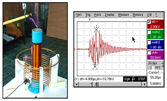
Figure 15.
Test for the Lp coil at a 90-degree angle and the wave that was used to calculate the Lp at a 90-degree angle.
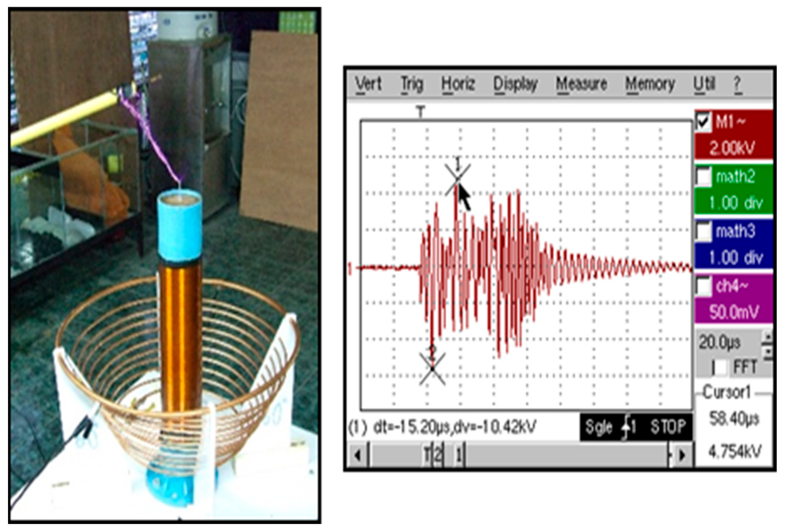
Figure 16 shows the frequency signal generated from the output of the Tesla transformer at a 60-degree angle is dt = −15.20 μs and dv = −10.42 kV.

Figure 16.
Test for the Lp coil at a 60-degree angle and the wave used to calculate the Lp at a 60-degree angle.
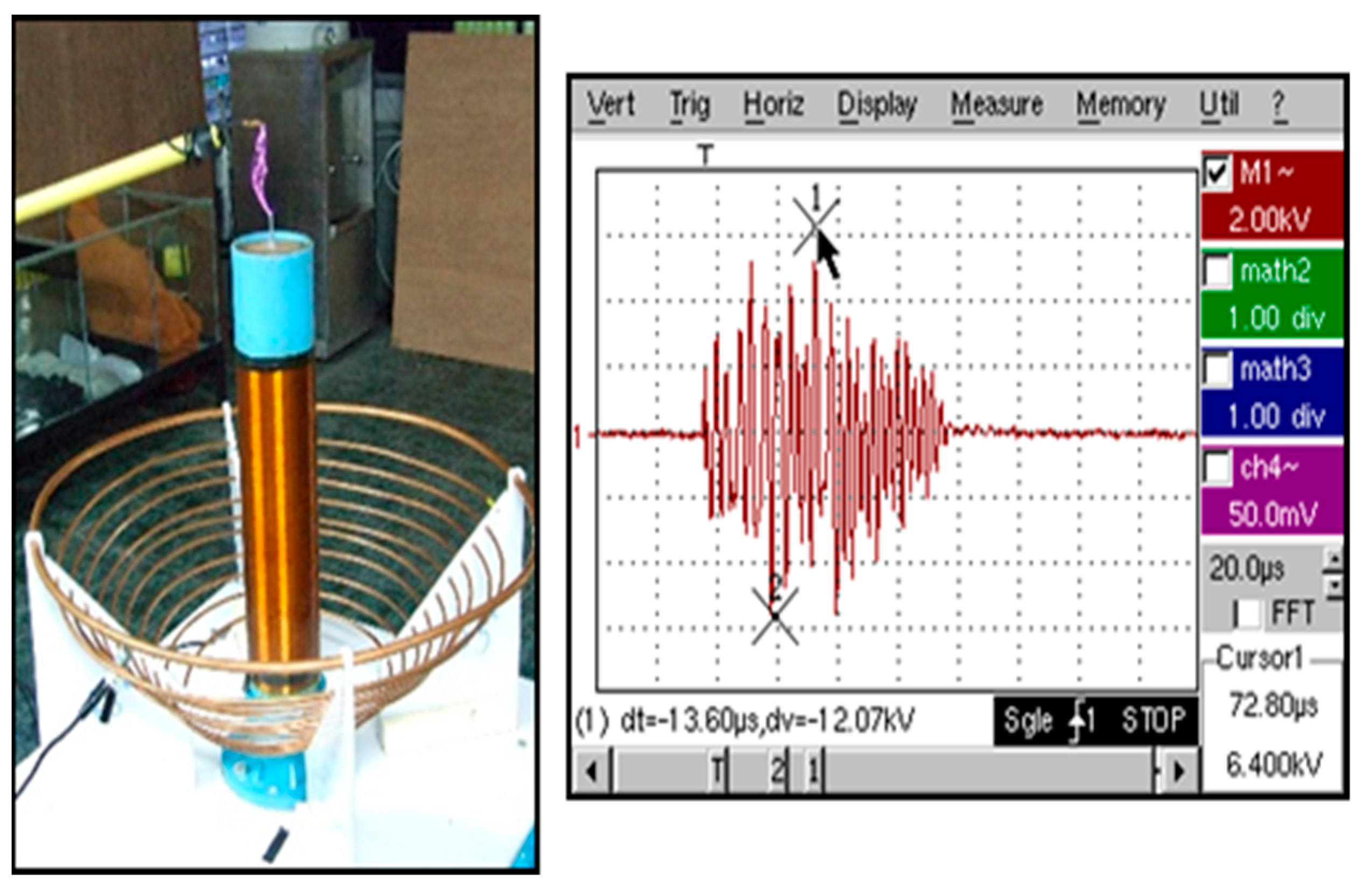
Figure 17 shows the frequency signal generated from the output of the Tesla transformer at a 45-degree angle is dt = −13.60 μs and dv = −12.07 kV.

Figure 17.
Test for the Lp coil at a 45-degree angle and the wave used to calculate the Lp at a 45-degree angle.
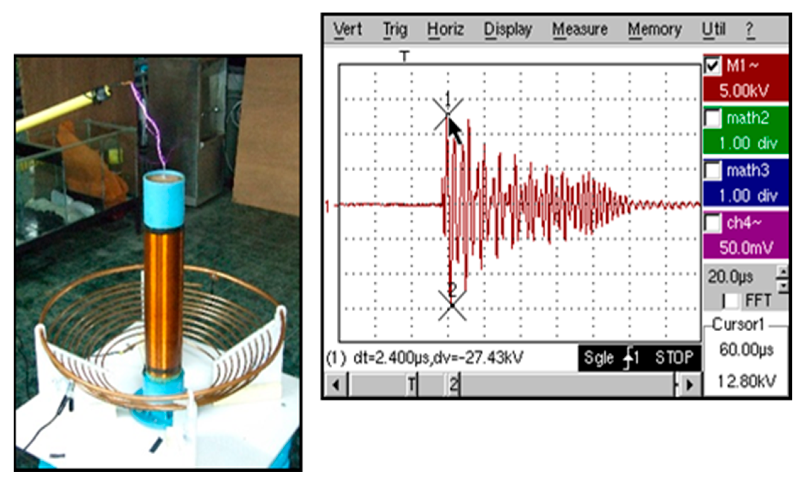
Figure 18 shows the frequency signal generated from the output of the Tesla transformer at a 30-degree angle is dt = 2.40 μs and dv = −27.43 kV.
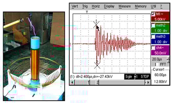
Figure 18.
Test for the Lp coil at a 30-degree angle and the wave used to calculate the Lp at a 30-degree angle.
Figure 19 shows the frequency signal generated from the output of the Tesla transformer at a 0-degree angle is dt = −30.00 μs and dv = −10.61 kV.
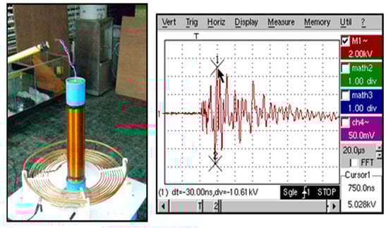
Figure 19.
Test for the Lp coil at a 0-degree angle and the wave used to calculate the Lp at a 0-degree angle.
A comparison of voltage flow from the placed primary coil is shown in Figure 20.
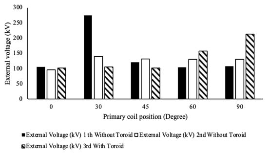
Figure 20.
Comparison of voltage flow from the placed primary coil.
Figure 21 shows the angle with the highest and lowest external frequency 1st without toroid is 60, and 0 degree, respectively. The angle with the highest and lowest external frequency 2nd without toroid is 90, and 30 degree, respectively. The angle with the highest and lowest external frequency 3rd with toroid is 90, and 60 degree, respectively.
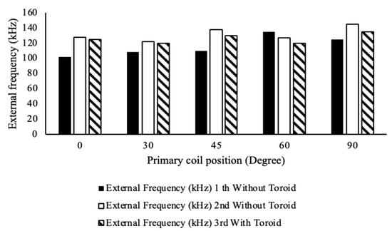
Figure 21.
Comparison of the external frequency with the primary coil placement.
Figure 22 shows the maximum of electricity field model testing by using FEMLAB program is 90 degree.
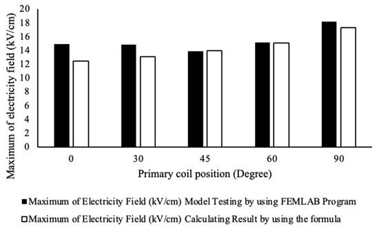
Figure 22.
Comparison of the electric field distribution model between primary coil (Lp) and secondary coil.
According to the results of the Tesla transformer testing and the electric field model designed for the placement of low- and high-voltage coils, the testing was conducted three times. The selection would be made by using the distribution impulse indicated in the adjustment atmosphere. The primary coil is placed at the same point, with eight rounds of primary coil binding at different angles, as shown in Table 3 and Table 4. It would seem that, at this point, the distribution voltage would be almost the same amount as the model at 120 kV 120 kHz, with the rounding of the primary coil (Lp) being close to the higher value in the model. According to the comparison, it can be concluded that placing the primary coil (Lp) at an angle from the floor results in the internal voltage and high electric field stress being more suitable than other models.
Table 3.
Comparing voltage that flows out of the placed primary coil at the adjusted position from round 8 for each type.
Table 4.
Comparison of the external frequency with the primary coil placement at the adjusted position with 8-round binding for each type.
Table 5 shows the model testing by using FEMLAB program is 18.23 kV/cm. (90 degree).
Table 5.
Comparison of the results of distribution electricity.
7. Conclusions
To study the effect of the high-voltage transformer induction and high frequency for finding suitable dimensions, the process would start by determining the transformer’s external impulse and frequency. The characteristics of coil induction (the suitable dimensions for placing the low-voltage coil (Lp) in several positions) and the model values were used in FEMLAB. The values obtained from the simulation would be used for comparison and analysis with the test results from the high-voltage, high-frequency transformer that was created. The analysis of several parameters suggests that, to position the Lp coil at the most suitable angle, it should be positioned at a 60-degree angle, according to this research.
Author Contributions
Conceptualization, S.N. and N.R.; Methodology, S.N. and N.R.; Validation, N.R.; Investigation, S.N. and N.R.; Writing—original draft, S.N.; Writing—review and editing, N.R. and S.N. All authors have read and agreed to the published version of the manuscript.
Funding
This research received no external funding.
Data Availability Statement
The study’s original contributions are included within the article, and any further inquiries can be directed to the corresponding authors.
Acknowledgments
The authors would like to express their sincere thanks to the Rajamangala University of Technology Phra Nakhon (RMUTP), Thailand, for their support.
Conflicts of Interest
The authors declare no conflicts of interest.
References
- ANSI C29.1-2018; Test Methods for Electrical Power Insulators. ANSI: Washington, DC, USA, 2018.
- Rigot, V.; Phulpin, T.; Sakly, J.; Sadarnac, D. A New 7 kW Air-Core Transformer at 1.5 MHz for Embedded Isolated DC/DC Application. Energies 2022, 15, 5211. [Google Scholar] [CrossRef]
- Denicolai, M. Tesla Transformer for Experimentation and Research. Ph.D. Thesis, Helsinki University of Technology, Espoo, Finland, 2001. [Google Scholar]
- Surwade, R.; Patil, H.; Parit, A.; Muley, S. Design of tesla coil. Int. Res. J. Eng. Technol. IRJET 2017, 4, 1543–1545. [Google Scholar]
- Abbasi, A.; Khanzade, M.H. Analysis of Dual Resonant Solid State Tesla Transformer. Int. J. Mod. Eng. Res. IJMER 2013, 3, 3456–3460. [Google Scholar]
- Tanwar, N.; Kumar, M.R.; Naidu, R.C. Design of Solid State Tesla Coil With Music Playback Functionality. IEEE Access 2024, 12, 14285–14297. [Google Scholar] [CrossRef]
- Hernanda, G.N.S.; Asfani, D.A.; Negara, I.M.Y.; Firdaus, M.Y.; Fatahillah, S.B.; Febrianti, A. Comparison of insulation testing in laboratory using solid-state-based tesla high-frequency voltage generation. Int. J. Innov. Comput. Inf. Control 2023, 19, 1265–1279. [Google Scholar]
- Woratipromma, S. Study and Analysis of a Design and Construction of Solid State Tesla Transformer Rated 100 kV 150 kHz. Master’s Thesis, Department of Electronics Engineering, Rajamangala University of Technology Thanyaburi, Pathum Thani, Thailand, 2014. [Google Scholar]
- Rahman, S.; Khan, S. The USB Powered Miniature Tesla coil, with Filament bulb, Fluorescent lamp and Discharge to Body. In Proceedings of the 2022 IEEE International IOT, Electronics and Mechatronics Conference (IEMTRONICS), Toronto, ON, Canada, 1–4 June 2022. [Google Scholar]
- Krbal, M.; Siuda, P. Design and construction solution of laboratory Tesla coil. In Proceedings of the 2015 16th International Scientific Conference on Electric Power Engineering (EPE), Kouty nad Desnou, Czech Republic, 20–22 May 2015. [Google Scholar]
- Kolchanova, V.A. Computational modeling of the Tesla coil parameters. In Proceedings of the 8th International Scientific and Practical Conference of Students, Post-Graduates and Young Scientists Modern Technique and Technologies, 2002, MTT 2002, Tomsk, Russia, 12 April 2002. [Google Scholar]
- Rana, M.S.; Pandit, A.K. Design and Construction of a Tesla Transformer by using Microwave Oven Transfer for Experimentation. Innov. Syst. Des. Eng. 2014, 5, 15–22. [Google Scholar]
- Tesla, N. Apparatus for Transmitting Electrical Energy. US Patent No. 1119732, 1 December 1914. [Google Scholar]
- Purcell, E.M.; Morin, D.J. Electricity and Magnetism, 3rd ed.; Cambridge University Press: New York, NY, USA; pp. 15–16.
- Lantharthong, T.; Nedphograw, S.; Hiranvarodom, S.; Apiratikul, P. Analysis of Electric field and Modeling Design of High Voltage Cable terminators for PD Testing Using SF6 Insulator. In Proceedings of the International Conference on Electrical Engineering 2008, Okinawa, Japan, 6–10 July 2008. [Google Scholar]
- Plangklang, B.; Apiratikul, P.; Phumkittipich, K. Development of Low-Cost Tesla Transformer for High Performance Testing 115 kV Line Post Insulator. J. Eng. RMUTT 2010, 8, 69–78. [Google Scholar]
- Santos, N.; Chaves, M.; Gamboa, P.; Cordeiro, A.; Santos, N.; Pinto, S.F. High Frequency Transformers for Solid-State Transformer Applications. Appl. Sci. 2023, 13, 7262. [Google Scholar] [CrossRef]
- Plangklang, B.; Apiratikul, P.; Boonchiam, P. A Low-Cost High Performance Tesla Transformer for testing 115 kV Line Post Insulator. In Proceedings of the 2006 International Conference on Power System Technology, Chongqing, China, 22–26 October 2006. [Google Scholar]
- Craven, R.M. A Study of Secondary Winding Designs for the Two-Coil Tesla Transformer. Ph.D. Thesis, Department of Electronics Engineering, Loughborough University, Loughborough, UK, 2014. [Google Scholar]
- Jana, S.; Biswas, P.K.; Babu, T.S.; Alhelou, H.H. An Improved Parametric Method for Selecting Different Types of Tesla Transformer Primary Coil to Construct an Artificial Lightning Simulator. IEEE Access 2023, 11, 22174–22186. [Google Scholar] [CrossRef]
- Pongsathit, W.; Yutthagowith, P.; Limcharoen, W. Solid state tesla transformer for flashover test on suspension insulators. In Proceedings of the 2017 International Symposium on Electrical Insulating Materials (ISEIM), Toyohashi, Japan, 11–15 September 2017. [Google Scholar]
- Nedphograw, S. High Voltage Engineering; Rajamangala University of Technology Phra Nakhon: Bangkok, Thailand, 2018. [Google Scholar]
- Thongkeaw, S.; Nedphograw, S.; Plangklang, B.; Apiratikul, P. The Analysis of high-Voltage Electric Field Stress in Lp and Ls coils of Tesla Transformer for studying the efficiency design. In Proceedings of the IAENG International Conference on Electrical Engineering (ICEE’08), Hong Kong, 19–21 March 2008. [Google Scholar]
- Sangsa-ard, S. High Voltage Engineering, 2nd ed.; Chulalongkorn University: Bangkok, Thailand, 1985. [Google Scholar]


Disclaimer/Publisher’s Note: The statements, opinions and data contained in all publications are solely those of the individual author(s) and contributor(s) and not of MDPI and/or the editor(s). MDPI and/or the editor(s) disclaim responsibility for any injury to people or property resulting from any ideas, methods, instructions or products referred to in the content. |
© 2025 by the authors. Licensee MDPI, Basel, Switzerland. This article is an open access article distributed under the terms and conditions of the Creative Commons Attribution (CC BY) license (https://creativecommons.org/licenses/by/4.0/).