1. Introduction
In light of the depletion of fossil fuels and global warming, the use of renewable energy sources has been treated as a crucial step for carbon emission reduction. As one of the main forms of solar energy utilization, distributed photovoltaic (PV) possesses advantages such as renewability and zero pollution and has received policy support and rapid development in many countries [
1,
2].
However, as the PV output highly depends on weather conditions, employing solar energy as a significant source of energy resources increases the difficulty of power system supply and demand balance scheduling management [
3]. Weather parameters such as solar irradiance, atmospheric temperature, cloud cover, wind pressure, and humidity are unpredictable and ungovernable. The random, volatile, and intermittent nature of PV power generation caused by meteorology significantly impacts load characteristics and power flow distribution in the distribution network, potentially leading to overvoltage issues in certain scenarios. Solar PV forecasting is a pivotal factor to support reliable and cost-effective grid operation and control [
4].
By utilizing PV power forecasting, it is possible to anticipate the power output of photovoltaic systems over a specific period. Such forecasts enable grid operators to optimize scheduling plans, such as allocating reserve capacity efficiently, adjusting the output of conventional generators, and fine-tuning electricity trading strategies [
5]. This helps mitigate the uncertainties caused by PV power fluctuations. Additionally, forecasting provides valuable references for real-time grid control, helping to prevent issues such as overvoltage or frequency deviations, thereby enhancing the stability and security of grid operations [
6,
7].
There are two main approaches for solar power forecasting. The first option consists of using analytical equations to model the PV system. The physical method studies the characteristics of PV power generation equipment and establishes the corresponding mathematical model for power forecasting. The meteorological and geological parameters used for physical mathematical models are usually measured by numerical weather prediction (NWP) or ground measurement devices. However, physical methods require appropriate and frequently calibrated service facilities. Normally, most efforts are dedicated to obtain accurate irradiance forecasts, which is the main factor related to the power production. Contrarily, the second option consists of directly predicting the power output using statistical and machine learning methods. Unlike physical methods that rely on precise measurements and calibration, AI approaches can efficiently model complex spatial–temporal dependencies and learn a mapping relationship between input and output, mainly focusing on nonlinear mapping models. This makes them highly effective in capturing the inherent variability and uncertainty in PV power generation. Additionally, forecasts can also be made based on a mix of both methods [
8]. PV forecasting can also be categorized based on the time scale of the prediction, with different time scales favoring distinct forecasting methods. In this work, we focus on regional short-term PV power forecasts with a 15-min lead time.
Statistical models rely solely on external data and do not require any internal information about the system. As a data-driven approach, they analyze historical data to uncover relationships and predict the future behavior of the plant. Therefore, the quality of historical data is crucial for producing accurate forecasts. These models have demonstrated better performance than analytical models in accurately predicting PV output [
6].
Machine learning can be adapted to new data, discovering hidden patterns and correlations in the data, which improves the accuracy of the prediction. The literature [
9] applies support vector regression (SVR) to evaluate the ability of machine learning approaches to serve as an alternative and a complement to physical forecasting models. The predictive performance of Artificial Neural Network (ANN) models has been experimentally verified to outperform Auto-Regressive Integrated Moving Average (ARIMA) models under complex situations. The following references provide a detailed discussion of similar methods [
10,
11,
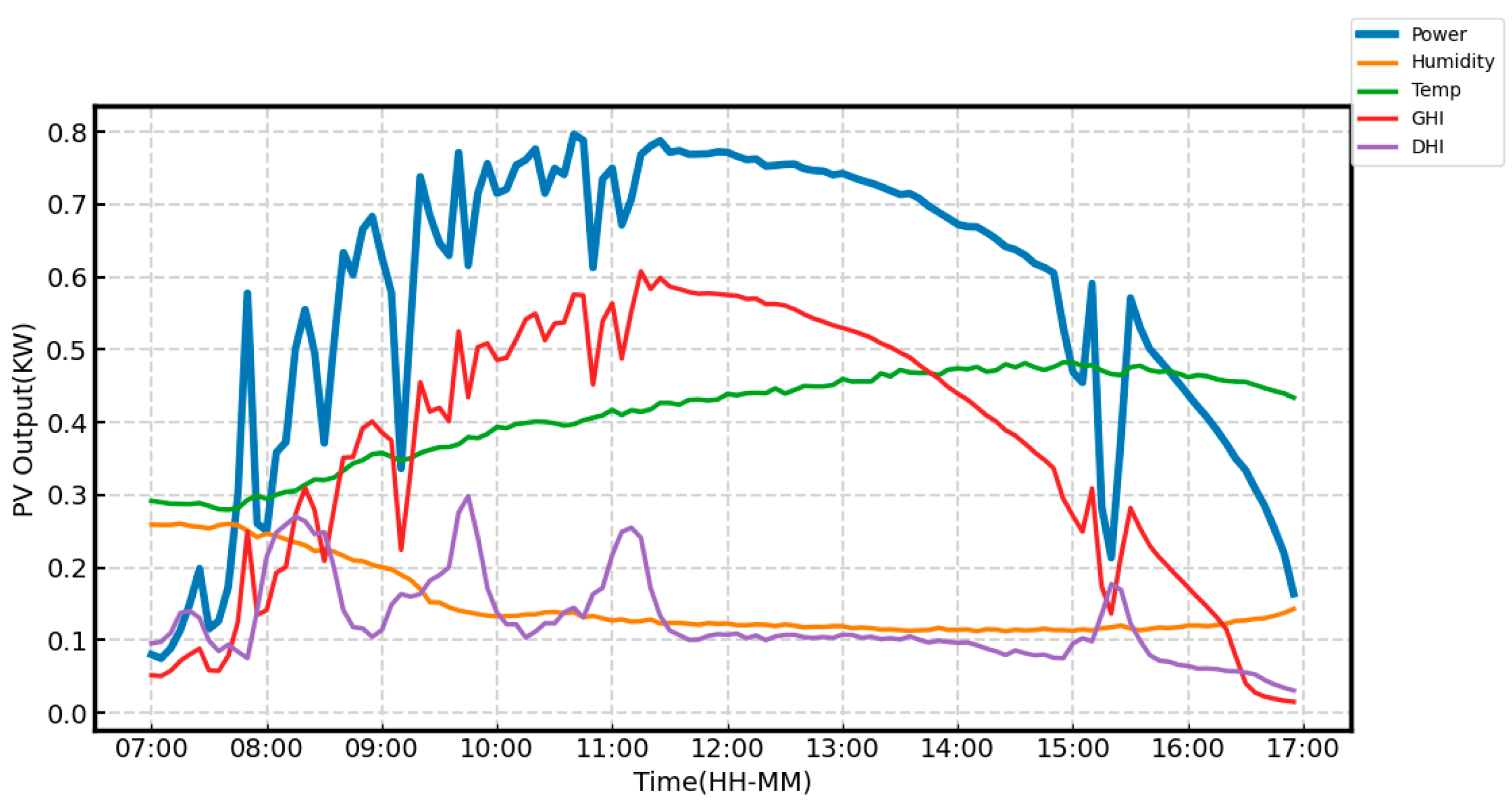
12]. By using weather data as input, machine learning models can leverage these external factors to better predict PV output, leading to more accurate and reliable forecasting. The most commonly used meteorological data include global horizontal radiation, diffuse horizontal radiation, ambient temperature, relative humidity, and wind speed. The literature [
13] utilizes the relationship between photovoltaic (PV) power output and meteorological factors to group similar patterns or behaviors, and then performs forecasting on each cluster. By segmenting the data into clusters with similar characteristics, this method enhances the accuracy of the predictions. Due to the limitations of machine learning, such as its limited ability to handle complex nonlinear relationships, poor adaptability to large-scale data, and shortcomings in feature extraction, deep learning has been introduced as a solution. Deep learning, through multi-layer neural networks, can automatically extract high-dimensional features from the data and capture more complex patterns, thereby improving the accuracy and stability of predictions.
Building forecasting models with stronger learning capabilities is an effective approach to improve the accuracy of PV power forecasting. In recent years, with the continuous development of deep learning algorithms, their applications in power forecasting have become increasingly widespread. Convolutional neural networks (CNNs) and LSTMs are two typical representative algorithms in deep learning. The core mechanism of CNNs involves convolutional layers, which apply filters (kernels) to input data to extract hierarchical features. These filters are learnable parameters that slide over the input, performing convolution operations to capture local patterns like edges, textures, or temporal correlations. This local connectivity and shared weights significantly reduce the number of parameters compared to fully connected networks, improving computational efficiency. The LSTM architecture introduces memory cells and a gating mechanism, which regulate the flow of information through three types of gates: input, forget, and output gates. The input gate determines how much of the new input information should be stored in the memory cell, the forget gate controls which parts of the memory to discard, and the output gate determines the information to be passed to the next layer. This literature [
14] combines CNNs and LSTMs for multivariate datasets, incorporating more features that impact photovoltaic power plant production (e.g., weather features). The forecasting time range varies from one day to one week ahead, and the results demonstrate that this approach achieves more accurate predictions compared to traditional LSTM models. This literature [
15] employs the Transformer architecture to extract features from multichannel sequences and dynamically integrate contextual information. The model’s predictive performance is evaluated across different seasons. Readers can find an in-depth analysis in the related studies [
16,
17,
18,
19,
20].
Many researchers also focus on extracting features from time series data before leveraging high-performance models for prediction. The literature [
21] combines sequence decomposition methods and deep learning models to propose a model that can significantly improve the accuracy of PV power prediction. Empirical Mode Decomposition (EMD) is widely used in PV forecasting due to its ability to handle nonlinear and nonstationary data by adaptively decomposing it into Intrinsic Mode Functions (IMFs), enabling noise reduction, feature extraction, and multiscale analysis. However, it faces challenges such as mode mixing, end effects, high computational cost, sensitivity to noise, and a lack of theoretical foundation.
Researchers employ methods such as grid search, random search, Bayesian optimization, evolutionary algorithms, gradient-based optimization, and automated tuning tools, combined with empirical heuristics, to efficiently set hyperparameters for machine learning models, aiming to optimize both performance and efficiency. In articles [
22,
23], the GA (Genetic Algorithm) and PSO (Particle Swarm Optimization) algorithms are used for hyperparameter optimization. GA, inspired by natural selection, evolves solutions through selection, crossover, and mutation, making it effective for complex, high-dimensional problems. PSO, on the other hand, iteratively refines hyperparameters based on previous evaluations, offering a more efficient search and faster convergence compared to traditional methods. For the implementation and application of similar approaches, the following key papers are recommended [
24,
25].
Despite the continuous emergence of various advanced models, single-point predictions still have certain limitations. The errors in machine learning models often stem from data noise, model bias, and uncertainties during the training process. In single-point predictions, these errors cannot be fully captured or quantified, which impacts the reliability and accuracy of the predictions. To mitigate the errors of single-point predictions, probabilistic models can be used instead of deterministic models. Probabilistic models provide estimates of prediction uncertainty, helping us better understand the confidence of the predictions and make more robust decisions. Furthermore, methods such as ensemble learning, cross-validation, and uncertainty quantification can also enhance prediction accuracy and reduce the bias associated with single-point predictions.
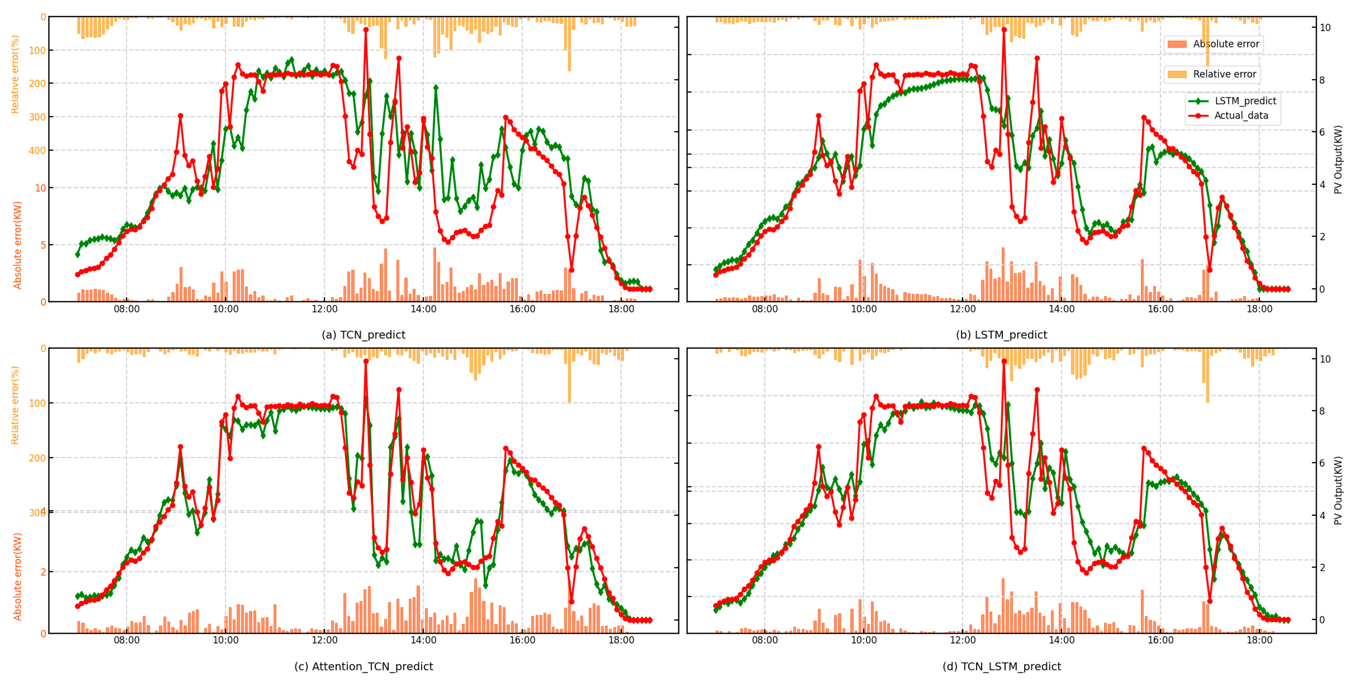
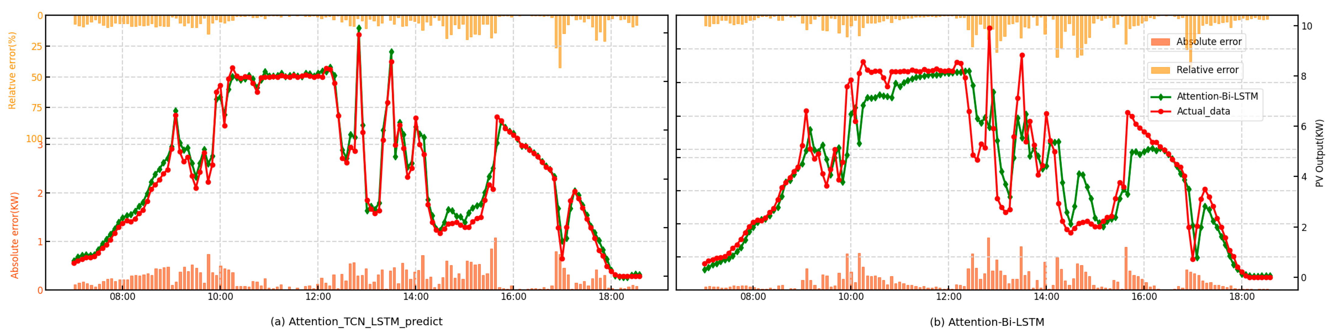
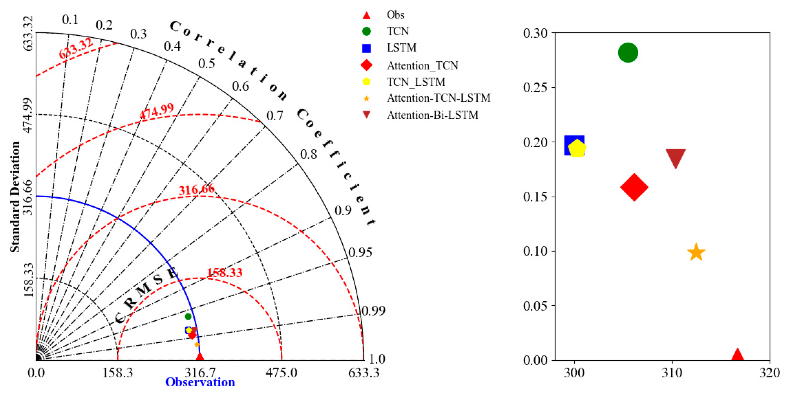
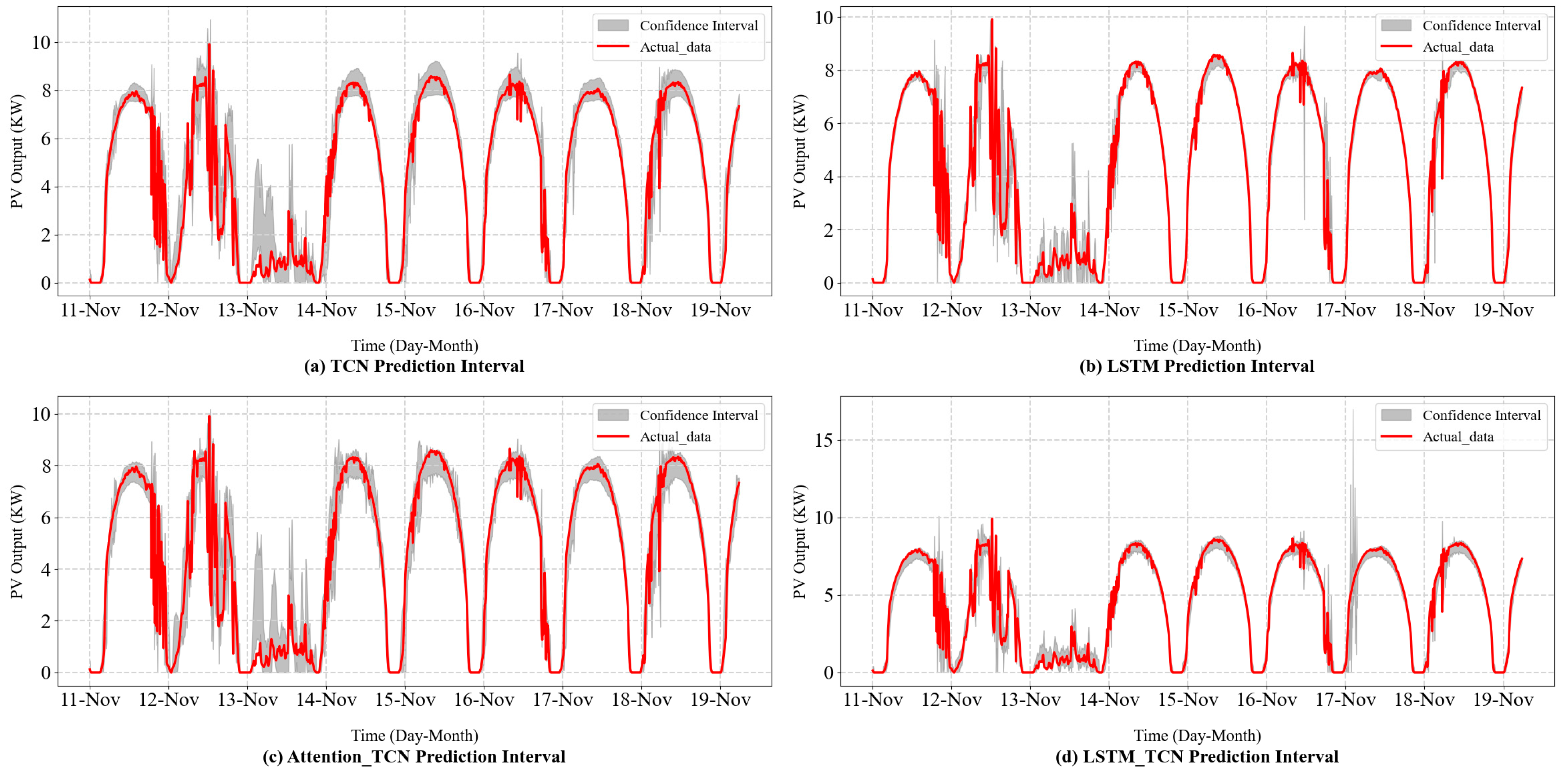
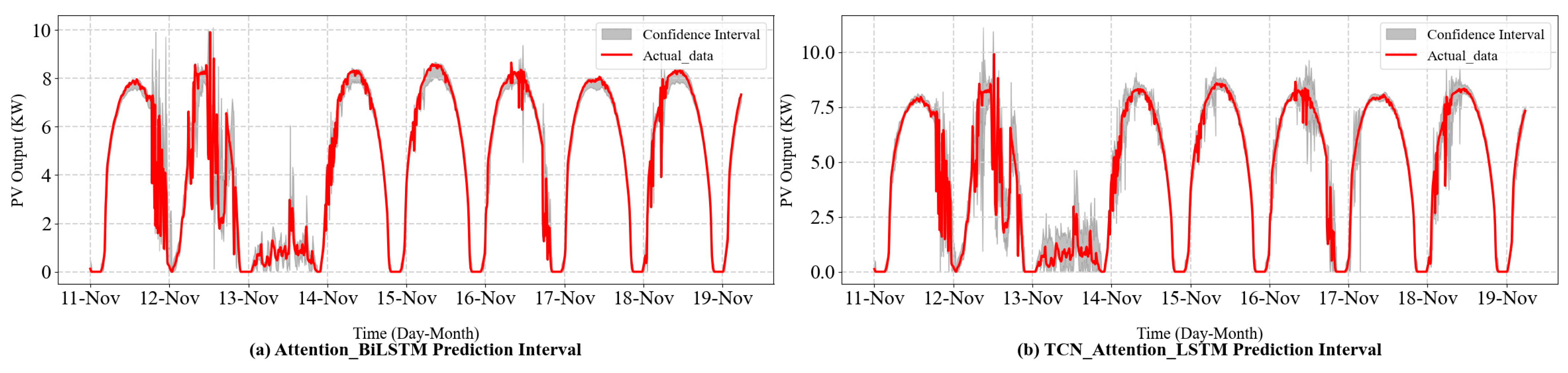
This paper proposes a hybrid Attention-TCN-LSTM model and demonstrates its superiority over traditional algorithms such as Bi-LSTM through comprehensive comparisons. By incorporating the bootstrap technique for interval prediction, the proposed method enhances the reliability and practicality of the predictions. The feasibility and effectiveness of the approach are further validated using interval prediction metrics, providing robust evidence of its potential in addressing the challenges of accurate and reliable interval prediction.
2. Methodology
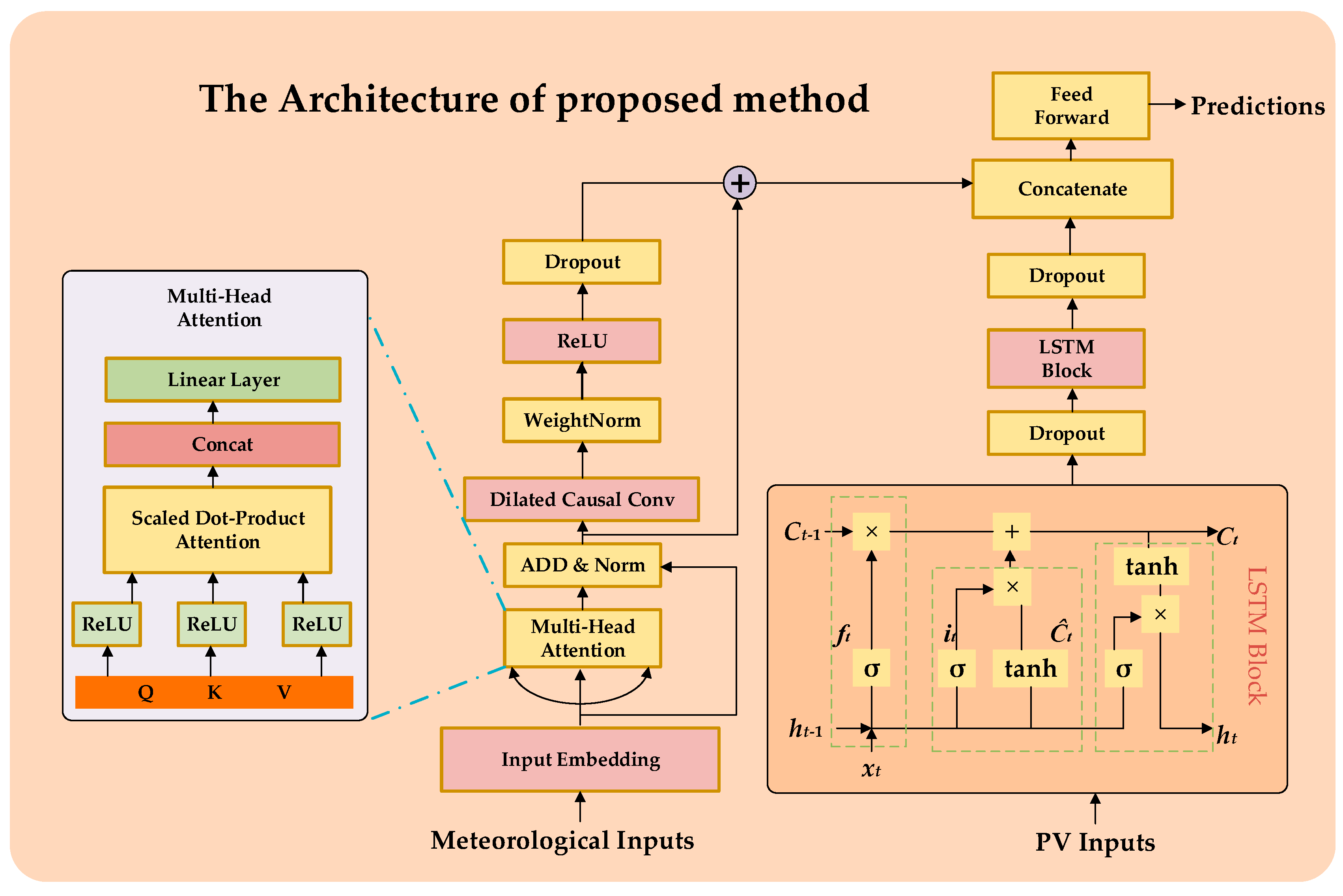
In the proposed framework, the PV output sequence characteristics learned by the LSTM are integrated with meteorological sequence characteristics extracted by the Attention-TCN module. This combination allows the model to jointly leverage the temporal patterns in PV output and the interdependencies among meteorological factors to enhance the accuracy of PV power prediction across various time horizons. The proposed hybrid model is developed in Python using Keras (version 2.11.0), a deep learning library that operates on TensorFlow.
Figure 1 illustrates the architecture of the proposed method. In the following paragraphs, we discuss several important components and the concepts related to interval prediction.
An LSTM is a type of recurrent neural network (RNN) specifically designed to overcome the vanishing gradient problem, allowing it to model both short-term and long-term dependencies in sequential data. In the context of PV power prediction, the historical output sequence exhibits strong temporal correlations, making the LSTM an ideal choice for extracting meaningful temporal features. The LSTM cell operates by maintaining a cell state
and a hidden state
, which are updated at each time step
based on the input
. The operations of the LSTM can be expressed as:
where
,
, and
represent the forget gate, input gate, and output gate, respectively.
denotes the sigmoid activation function,
is the hyperbolic tangent function,
and
are the learnable weights and biases, and
represents element-wise multiplication. By using these gating mechanisms, the LSTM selectively updates and retains information over time, ensuring that the extracted features effectively encode the temporal dynamics of the PV power output sequence. The hidden state
, which also serves as the output of the LSTM cell at time step
of the LSTM layer, serves as a representation of the historical PV power patterns, which is subsequently combined with features extracted from meteorological data. The size of the hidden state, denoted as
Hidden State Size, is a key parameter in determining the model’s capacity to capture complex patterns. It defines the number of units or neurons in the hidden layer, influencing how much information the model can store and process at each time step. A larger
Hidden State Size allows the model to store more information and capture more complex relationships, enabling it to better learn long-term dependencies and intricate patterns in the data. Conversely, a smaller
Hidden State Size might restrict the model’s ability to remember long-term dependencies, which can affect its performance on tasks with complex temporal dynamics.
The self-attention mechanism of Transformer module dynamically weighs the contribution of each feature, enabling the model to learn a comprehensive representation of the meteorological context [
26]. The self-attention mechanism can be expressed as:
where
,
and
are the query, key, and value matrices derived from the input features. The
Head Size is defined as
, which is the dimension of the query and key vectors in each attention head. For each attention head, the queries, keys, and values are projected using distinct learned weight matrices, and attention is computed in parallel across the heads. After the attention scores are calculated for each head, the results are concatenated and passed through a final linear layer to produce the output of the multi-head attention mechanism. This allows the model to capture different types of dependencies across the sequence simultaneously, with each head focusing on a different aspect of the input data. The Number of Heads (
Num Heads) defines how many separate attention mechanisms the model will use. Increasing the Number of Heads enables the Transformer to capture more diverse relationships between different parts of the input sequence. Furthermore, after the multi-head attention mechanism, the output is passed through a feed-forward neural network (FFN) at each time step. The FFN consists of two linear layers with a nonlinear activation function in between, and the dimensionality of the hidden layer is controlled by a parameter called
Feed-Forward Dimension (
FF Dim). By leveraging this mechanism, the Transformer computes feature dependencies across the multivariate inputs, generating an enhanced representation
for each time step
.
While the self-attention mechanism focuses on inter-feature dependencies, the TCN module is designed to capture temporal patterns in the sequential data. Using causal and dilated convolutions, the TCN ensures efficient modeling of both short-term and long-term dependencies while respecting the temporal causality of PV output prediction [
27]. The output of the TCN at each time step can be formulated as:
where
is the output at time
,
is the convolutional kernel,
is the input under the receptive field of the kernel,
is the bias,
represents the convolution operation, and
is the activation function (e.g., ReLU). In the TCN, the
Filters represent the number of convolutional kernels applied in each layer. Each filter learns a unique set of patterns from the input sequence, with more filters allowing the TCN to extract a richer and more diverse set of features. The
Kernel Size determines the receptive field of the convolutional layer, i.e., how many time steps the network considers simultaneously when generating the output for a particular time step. A larger Kernel Size allows the network to capture broader temporal patterns, while a smaller Kernel Size focuses on more localized, short-term patterns. The integration of self-attention mechanism and the TCN ensures that both temporal and spatial (feature-wise) dependencies are jointly modeled. The overall output of the hybrid model for the PV power prediction task can be expressed as:
where
represents the historical meteorological time series and
denotes the historical PV power output sequence. The
function models the complex interdependencies among meteorological factors, while
captures the temporal dynamics within the meteorological sequence. Simultaneously,
extracts temporal features from the PV power output sequence. The operator
indicates feature fusion, such as concatenation or addition, to integrate the outputs from both modules. This
serves as a comprehensive representation of the temporal and spatial patterns in the input data, forming the basis for subsequent PV power prediction.
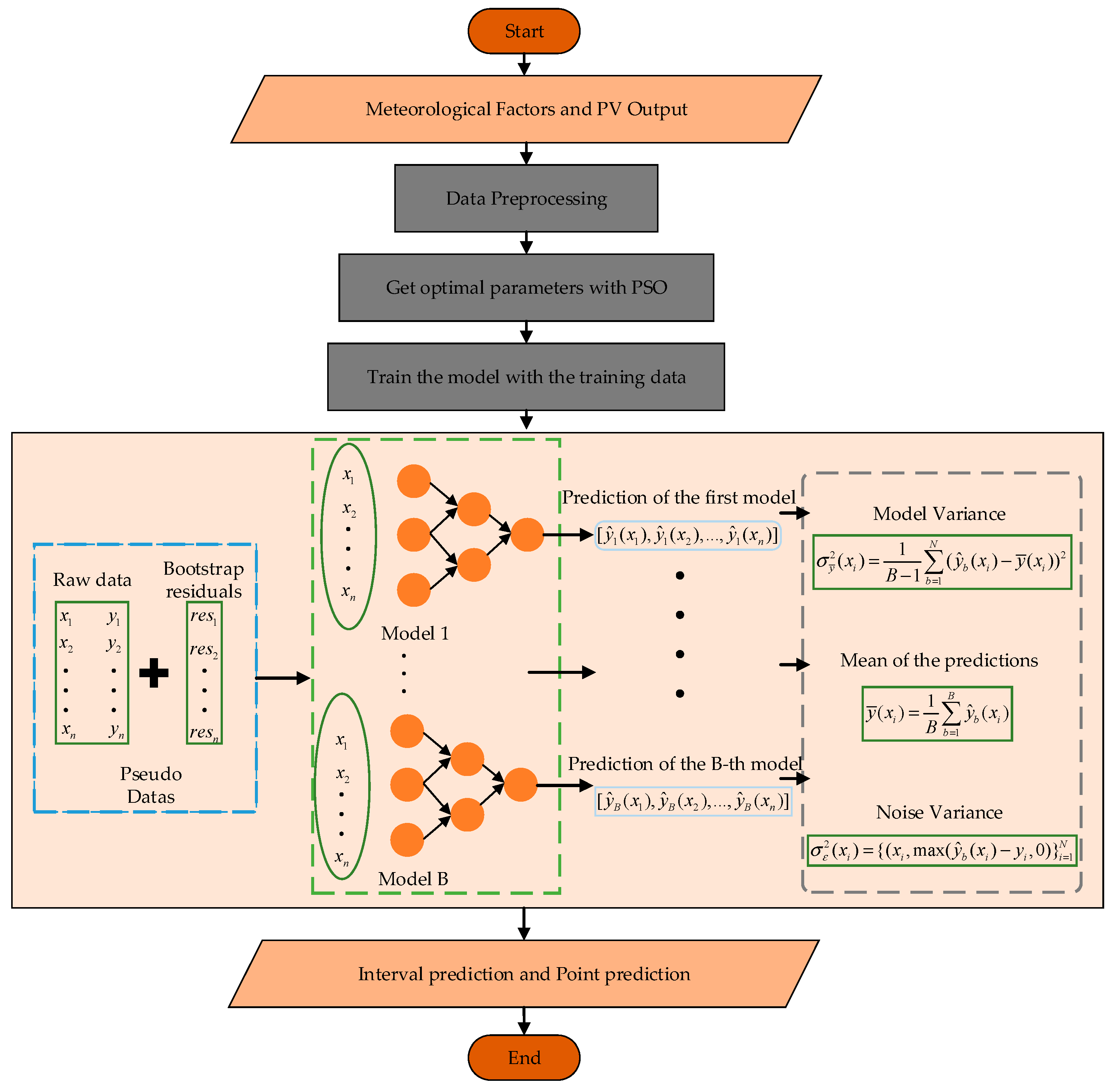
The uncertainty in prediction results can be attributed to two main sources of variance: model variance and noise variance. Model variance reflects the uncertainty in the model’s predictions due to its structure, parameters, and the potential for overfitting or underfitting. It indicates how much the predictions might change if the model was trained on different data or initialized differently. On the other hand, noise variance captures the inherent randomness or unpredictability in the data that the model cannot explain, such as environmental fluctuations, measurement errors, or other external factors. Together, these variances are used to generate more reliable prediction intervals, providing a com-prehensive view of the uncertainty in both the model’s predictions and the underlying data.
Interval prediction is a method used to predict the uncertainty of a variable over a future time span. This approach estimates the potential range of possible future values and presents the prediction results in the form of an interval at a given confidence level, thereby accurately reflecting the uncertainty of the prediction. The interval is accompanied by a confidence level (e.g., 95% or 99%), meaning that the predicted value has a certain probability of being within the interval.
In this study, we employ the bootstrap method not only to assess the uncertainty of PV power predictions but also to enhance the model’s performance by reconstructing the input data using prediction biases. The primary goal is to improve the prediction accuracy and construct reliable prediction intervals that can capture the inherent variability in PV power generation [
28]. The process begins by training the PV power prediction model on the original dataset. After obtaining the model’s initial predictions
, the prediction bias for each instance is calculated as the difference between the true value
and the predicted value
, i.e., the prediction bias:
Next, the model’s input data are reconstructed by adding the prediction bias back to the corresponding input features, which is performed in the following manner for each instance:
where
is the original input feature vector, and
is the reconstructed input data. This reconstruction process aims to account for the systematic error introduced by the model and helps in refining the predictive accuracy.
To compute the model’s error and build confidence intervals for PV power predictions, the bootstrap resampling technique is applied to the reconstructed data. The procedure involves generating multiple bootstrap samples
from the reconstructed dataset and retraining the model on each sample:
where
represents the reconstructed input data and
is the corresponding output. The model is trained on each bootstrap sample, and predictions
are generated for all
bootstrap iterations.
Once the predictions for all bootstrap iterations are available, the final prediction
is obtained as the average of all predictions:
The model variance caused by the model itself during training can be calculated using the following formula:
The prediction interval for the PV power is constructed using the distribution of errors across all bootstrap iterations. The
confidence interval for the predictions is given by:
where
is the standard deviation of the predictions across all bootstrap samples, and
is the critical value for the desired confidence level
.
However, in practical engineering applications, the intervals constructed by the model variance do not meet the requirements of the application. To construct intervals that meet the requirements, estimating the noise variance is indispensable. Therefore, the noise variance can be estimated through a resampled dataset, and its expression is as follows:
where
represents the noise variance. However, since noise cannot be negative, the estimated noise variance
is given by:
Finally, the variance used to calculate the confidence interval should be the sum of the model variance and the noise variance. This approach allows for the creation of robust prediction intervals that reflect the variability of PV power output, providing both point predictions and reliable bounds for decision-making in PV power generation forecasting.


