Abstract
In response to the challenges posed by renewable energy integration, this study introduces a hybrid Attention-TCN-LSTM model for short-term photovoltaic (PV) power forecasting. The LSTM captures the sequence characteristics of PV output, which are then combined with the meteorological sequence features extracted by the Attention-TCN module. The model leverages the strengths of the TCN, the LSTM, and the self-attention mechanism to enhance prediction accuracy and construct reliable prediction intervals. Aiming to optimize both performance and efficiency, the PSO algorithm is used for hyperparameter optimization. Ablation studies and comparisons with other models confirm the effectiveness, accuracy and robustness of the proposed model. This hybrid approach contributes to improved renewable energy integration, offering a more stable and reliable energy supply. Future work will focus on incorporating intelligent systems for autonomous risk management and real-time control of dynamic PV output fluctuations.
1. Introduction
In light of the depletion of fossil fuels and global warming, the use of renewable energy sources has been treated as a crucial step for carbon emission reduction. As one of the main forms of solar energy utilization, distributed photovoltaic (PV) possesses advantages such as renewability and zero pollution and has received policy support and rapid development in many countries [1,2].
However, as the PV output highly depends on weather conditions, employing solar energy as a significant source of energy resources increases the difficulty of power system supply and demand balance scheduling management [3]. Weather parameters such as solar irradiance, atmospheric temperature, cloud cover, wind pressure, and humidity are unpredictable and ungovernable. The random, volatile, and intermittent nature of PV power generation caused by meteorology significantly impacts load characteristics and power flow distribution in the distribution network, potentially leading to overvoltage issues in certain scenarios. Solar PV forecasting is a pivotal factor to support reliable and cost-effective grid operation and control [4].
By utilizing PV power forecasting, it is possible to anticipate the power output of photovoltaic systems over a specific period. Such forecasts enable grid operators to optimize scheduling plans, such as allocating reserve capacity efficiently, adjusting the output of conventional generators, and fine-tuning electricity trading strategies [5]. This helps mitigate the uncertainties caused by PV power fluctuations. Additionally, forecasting provides valuable references for real-time grid control, helping to prevent issues such as overvoltage or frequency deviations, thereby enhancing the stability and security of grid operations [6,7].
There are two main approaches for solar power forecasting. The first option consists of using analytical equations to model the PV system. The physical method studies the characteristics of PV power generation equipment and establishes the corresponding mathematical model for power forecasting. The meteorological and geological parameters used for physical mathematical models are usually measured by numerical weather prediction (NWP) or ground measurement devices. However, physical methods require appropriate and frequently calibrated service facilities. Normally, most efforts are dedicated to obtain accurate irradiance forecasts, which is the main factor related to the power production. Contrarily, the second option consists of directly predicting the power output using statistical and machine learning methods. Unlike physical methods that rely on precise measurements and calibration, AI approaches can efficiently model complex spatial–temporal dependencies and learn a mapping relationship between input and output, mainly focusing on nonlinear mapping models. This makes them highly effective in capturing the inherent variability and uncertainty in PV power generation. Additionally, forecasts can also be made based on a mix of both methods [8]. PV forecasting can also be categorized based on the time scale of the prediction, with different time scales favoring distinct forecasting methods. In this work, we focus on regional short-term PV power forecasts with a 15-min lead time.
Statistical models rely solely on external data and do not require any internal information about the system. As a data-driven approach, they analyze historical data to uncover relationships and predict the future behavior of the plant. Therefore, the quality of historical data is crucial for producing accurate forecasts. These models have demonstrated better performance than analytical models in accurately predicting PV output [6].
Machine learning can be adapted to new data, discovering hidden patterns and correlations in the data, which improves the accuracy of the prediction. The literature [9] applies support vector regression (SVR) to evaluate the ability of machine learning approaches to serve as an alternative and a complement to physical forecasting models. The predictive performance of Artificial Neural Network (ANN) models has been experimentally verified to outperform Auto-Regressive Integrated Moving Average (ARIMA) models under complex situations. The following references provide a detailed discussion of similar methods [10,11,12]. By using weather data as input, machine learning models can leverage these external factors to better predict PV output, leading to more accurate and reliable forecasting. The most commonly used meteorological data include global horizontal radiation, diffuse horizontal radiation, ambient temperature, relative humidity, and wind speed. The literature [13] utilizes the relationship between photovoltaic (PV) power output and meteorological factors to group similar patterns or behaviors, and then performs forecasting on each cluster. By segmenting the data into clusters with similar characteristics, this method enhances the accuracy of the predictions. Due to the limitations of machine learning, such as its limited ability to handle complex nonlinear relationships, poor adaptability to large-scale data, and shortcomings in feature extraction, deep learning has been introduced as a solution. Deep learning, through multi-layer neural networks, can automatically extract high-dimensional features from the data and capture more complex patterns, thereby improving the accuracy and stability of predictions.
Building forecasting models with stronger learning capabilities is an effective approach to improve the accuracy of PV power forecasting. In recent years, with the continuous development of deep learning algorithms, their applications in power forecasting have become increasingly widespread. Convolutional neural networks (CNNs) and LSTMs are two typical representative algorithms in deep learning. The core mechanism of CNNs involves convolutional layers, which apply filters (kernels) to input data to extract hierarchical features. These filters are learnable parameters that slide over the input, performing convolution operations to capture local patterns like edges, textures, or temporal correlations. This local connectivity and shared weights significantly reduce the number of parameters compared to fully connected networks, improving computational efficiency. The LSTM architecture introduces memory cells and a gating mechanism, which regulate the flow of information through three types of gates: input, forget, and output gates. The input gate determines how much of the new input information should be stored in the memory cell, the forget gate controls which parts of the memory to discard, and the output gate determines the information to be passed to the next layer. This literature [14] combines CNNs and LSTMs for multivariate datasets, incorporating more features that impact photovoltaic power plant production (e.g., weather features). The forecasting time range varies from one day to one week ahead, and the results demonstrate that this approach achieves more accurate predictions compared to traditional LSTM models. This literature [15] employs the Transformer architecture to extract features from multichannel sequences and dynamically integrate contextual information. The model’s predictive performance is evaluated across different seasons. Readers can find an in-depth analysis in the related studies [16,17,18,19,20].
Many researchers also focus on extracting features from time series data before leveraging high-performance models for prediction. The literature [21] combines sequence decomposition methods and deep learning models to propose a model that can significantly improve the accuracy of PV power prediction. Empirical Mode Decomposition (EMD) is widely used in PV forecasting due to its ability to handle nonlinear and nonstationary data by adaptively decomposing it into Intrinsic Mode Functions (IMFs), enabling noise reduction, feature extraction, and multiscale analysis. However, it faces challenges such as mode mixing, end effects, high computational cost, sensitivity to noise, and a lack of theoretical foundation.
Researchers employ methods such as grid search, random search, Bayesian optimization, evolutionary algorithms, gradient-based optimization, and automated tuning tools, combined with empirical heuristics, to efficiently set hyperparameters for machine learning models, aiming to optimize both performance and efficiency. In articles [22,23], the GA (Genetic Algorithm) and PSO (Particle Swarm Optimization) algorithms are used for hyperparameter optimization. GA, inspired by natural selection, evolves solutions through selection, crossover, and mutation, making it effective for complex, high-dimensional problems. PSO, on the other hand, iteratively refines hyperparameters based on previous evaluations, offering a more efficient search and faster convergence compared to traditional methods. For the implementation and application of similar approaches, the following key papers are recommended [24,25].
Despite the continuous emergence of various advanced models, single-point predictions still have certain limitations. The errors in machine learning models often stem from data noise, model bias, and uncertainties during the training process. In single-point predictions, these errors cannot be fully captured or quantified, which impacts the reliability and accuracy of the predictions. To mitigate the errors of single-point predictions, probabilistic models can be used instead of deterministic models. Probabilistic models provide estimates of prediction uncertainty, helping us better understand the confidence of the predictions and make more robust decisions. Furthermore, methods such as ensemble learning, cross-validation, and uncertainty quantification can also enhance prediction accuracy and reduce the bias associated with single-point predictions.
This paper proposes a hybrid Attention-TCN-LSTM model and demonstrates its superiority over traditional algorithms such as Bi-LSTM through comprehensive comparisons. By incorporating the bootstrap technique for interval prediction, the proposed method enhances the reliability and practicality of the predictions. The feasibility and effectiveness of the approach are further validated using interval prediction metrics, providing robust evidence of its potential in addressing the challenges of accurate and reliable interval prediction.
2. Methodology
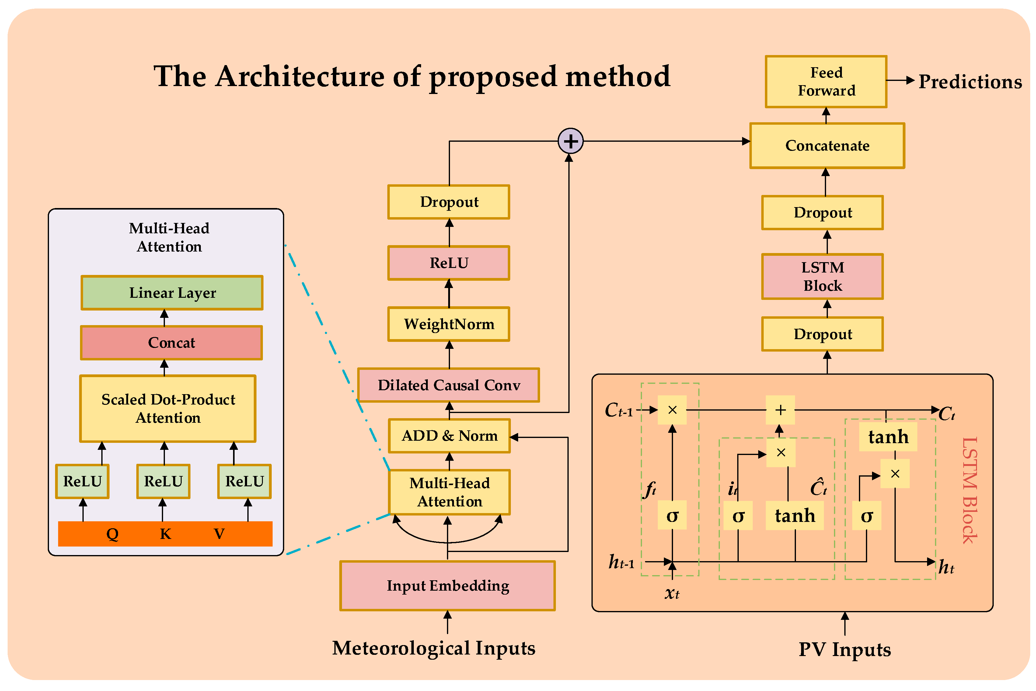
In the proposed framework, the PV output sequence characteristics learned by the LSTM are integrated with meteorological sequence characteristics extracted by the Attention-TCN module. This combination allows the model to jointly leverage the temporal patterns in PV output and the interdependencies among meteorological factors to enhance the accuracy of PV power prediction across various time horizons. The proposed hybrid model is developed in Python using Keras (version 2.11.0), a deep learning library that operates on TensorFlow. Figure 1 illustrates the architecture of the proposed method. In the following paragraphs, we discuss several important components and the concepts related to interval prediction.

Figure 1.
The architecture of proposed method.
An LSTM is a type of recurrent neural network (RNN) specifically designed to overcome the vanishing gradient problem, allowing it to model both short-term and long-term dependencies in sequential data. In the context of PV power prediction, the historical output sequence exhibits strong temporal correlations, making the LSTM an ideal choice for extracting meaningful temporal features. The LSTM cell operates by maintaining a cell state and a hidden state , which are updated at each time step based on the input . The operations of the LSTM can be expressed as:
where , , and represent the forget gate, input gate, and output gate, respectively. denotes the sigmoid activation function, is the hyperbolic tangent function, and are the learnable weights and biases, and represents element-wise multiplication. By using these gating mechanisms, the LSTM selectively updates and retains information over time, ensuring that the extracted features effectively encode the temporal dynamics of the PV power output sequence. The hidden state , which also serves as the output of the LSTM cell at time step of the LSTM layer, serves as a representation of the historical PV power patterns, which is subsequently combined with features extracted from meteorological data. The size of the hidden state, denoted as Hidden State Size, is a key parameter in determining the model’s capacity to capture complex patterns. It defines the number of units or neurons in the hidden layer, influencing how much information the model can store and process at each time step. A larger Hidden State Size allows the model to store more information and capture more complex relationships, enabling it to better learn long-term dependencies and intricate patterns in the data. Conversely, a smaller Hidden State Size might restrict the model’s ability to remember long-term dependencies, which can affect its performance on tasks with complex temporal dynamics.
The self-attention mechanism of Transformer module dynamically weighs the contribution of each feature, enabling the model to learn a comprehensive representation of the meteorological context [26]. The self-attention mechanism can be expressed as:
where , and are the query, key, and value matrices derived from the input features. The Head Size is defined as , which is the dimension of the query and key vectors in each attention head. For each attention head, the queries, keys, and values are projected using distinct learned weight matrices, and attention is computed in parallel across the heads. After the attention scores are calculated for each head, the results are concatenated and passed through a final linear layer to produce the output of the multi-head attention mechanism. This allows the model to capture different types of dependencies across the sequence simultaneously, with each head focusing on a different aspect of the input data. The Number of Heads (Num Heads) defines how many separate attention mechanisms the model will use. Increasing the Number of Heads enables the Transformer to capture more diverse relationships between different parts of the input sequence. Furthermore, after the multi-head attention mechanism, the output is passed through a feed-forward neural network (FFN) at each time step. The FFN consists of two linear layers with a nonlinear activation function in between, and the dimensionality of the hidden layer is controlled by a parameter called Feed-Forward Dimension (FF Dim). By leveraging this mechanism, the Transformer computes feature dependencies across the multivariate inputs, generating an enhanced representation for each time step .
While the self-attention mechanism focuses on inter-feature dependencies, the TCN module is designed to capture temporal patterns in the sequential data. Using causal and dilated convolutions, the TCN ensures efficient modeling of both short-term and long-term dependencies while respecting the temporal causality of PV output prediction [27]. The output of the TCN at each time step can be formulated as:
where is the output at time , is the convolutional kernel, is the input under the receptive field of the kernel, is the bias, represents the convolution operation, and is the activation function (e.g., ReLU). In the TCN, the Filters represent the number of convolutional kernels applied in each layer. Each filter learns a unique set of patterns from the input sequence, with more filters allowing the TCN to extract a richer and more diverse set of features. The Kernel Size determines the receptive field of the convolutional layer, i.e., how many time steps the network considers simultaneously when generating the output for a particular time step. A larger Kernel Size allows the network to capture broader temporal patterns, while a smaller Kernel Size focuses on more localized, short-term patterns. The integration of self-attention mechanism and the TCN ensures that both temporal and spatial (feature-wise) dependencies are jointly modeled. The overall output of the hybrid model for the PV power prediction task can be expressed as:
where represents the historical meteorological time series and denotes the historical PV power output sequence. The function models the complex interdependencies among meteorological factors, while captures the temporal dynamics within the meteorological sequence. Simultaneously, extracts temporal features from the PV power output sequence. The operator indicates feature fusion, such as concatenation or addition, to integrate the outputs from both modules. This serves as a comprehensive representation of the temporal and spatial patterns in the input data, forming the basis for subsequent PV power prediction.
The uncertainty in prediction results can be attributed to two main sources of variance: model variance and noise variance. Model variance reflects the uncertainty in the model’s predictions due to its structure, parameters, and the potential for overfitting or underfitting. It indicates how much the predictions might change if the model was trained on different data or initialized differently. On the other hand, noise variance captures the inherent randomness or unpredictability in the data that the model cannot explain, such as environmental fluctuations, measurement errors, or other external factors. Together, these variances are used to generate more reliable prediction intervals, providing a com-prehensive view of the uncertainty in both the model’s predictions and the underlying data.
Interval prediction is a method used to predict the uncertainty of a variable over a future time span. This approach estimates the potential range of possible future values and presents the prediction results in the form of an interval at a given confidence level, thereby accurately reflecting the uncertainty of the prediction. The interval is accompanied by a confidence level (e.g., 95% or 99%), meaning that the predicted value has a certain probability of being within the interval.
In this study, we employ the bootstrap method not only to assess the uncertainty of PV power predictions but also to enhance the model’s performance by reconstructing the input data using prediction biases. The primary goal is to improve the prediction accuracy and construct reliable prediction intervals that can capture the inherent variability in PV power generation [28]. The process begins by training the PV power prediction model on the original dataset. After obtaining the model’s initial predictions , the prediction bias for each instance is calculated as the difference between the true value and the predicted value , i.e., the prediction bias:
Next, the model’s input data are reconstructed by adding the prediction bias back to the corresponding input features, which is performed in the following manner for each instance:
where is the original input feature vector, and is the reconstructed input data. This reconstruction process aims to account for the systematic error introduced by the model and helps in refining the predictive accuracy.
To compute the model’s error and build confidence intervals for PV power predictions, the bootstrap resampling technique is applied to the reconstructed data. The procedure involves generating multiple bootstrap samples from the reconstructed dataset and retraining the model on each sample:
where represents the reconstructed input data and is the corresponding output. The model is trained on each bootstrap sample, and predictions are generated for all bootstrap iterations.
Once the predictions for all bootstrap iterations are available, the final prediction is obtained as the average of all predictions:
The model variance caused by the model itself during training can be calculated using the following formula:
The prediction interval for the PV power is constructed using the distribution of errors across all bootstrap iterations. The confidence interval for the predictions is given by:
where is the standard deviation of the predictions across all bootstrap samples, and is the critical value for the desired confidence level .
However, in practical engineering applications, the intervals constructed by the model variance do not meet the requirements of the application. To construct intervals that meet the requirements, estimating the noise variance is indispensable. Therefore, the noise variance can be estimated through a resampled dataset, and its expression is as follows:
where represents the noise variance. However, since noise cannot be negative, the estimated noise variance is given by:
Finally, the variance used to calculate the confidence interval should be the sum of the model variance and the noise variance. This approach allows for the creation of robust prediction intervals that reflect the variability of PV power output, providing both point predictions and reliable bounds for decision-making in PV power generation forecasting.
3. Implementation Procedure and Evaluation Indicators
3.1. Implementation Procedure of the Proposed Method
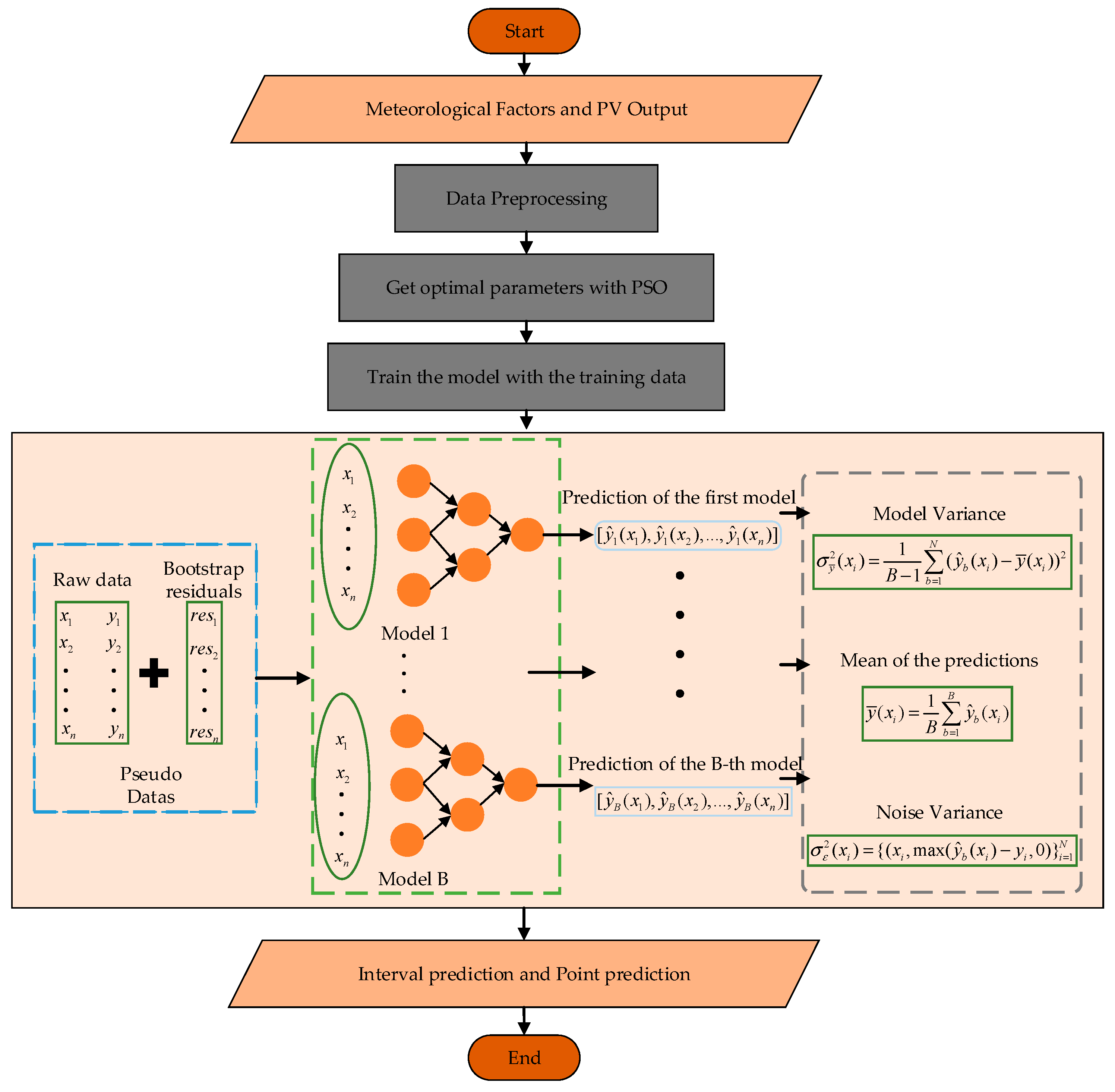
The implementation process of the proposed method is as follows. First, the input data, including historical photovoltaic output sequences and historical meteorological sequences, undergoes preprocessing. Next, the Particle Swarm Optimization algorithm is employed to determine the optimal hyperparameters, which are then used to train the point prediction model. Based on the bootstrap method, the model variance and noise variance are calculated to perform interval prediction, providing a more comprehensive assessment of the reliability of the point prediction results. The conceptual framework of this study is visually presented in Figure 2 for better clarity.

Figure 2.
The implementation procedure of the proposed method.
The bootstrap method involves creating multiple resampled datasets from the original training set through random sampling with replacement. Each resampled dataset is used to train an independent Attention-TCN-LSTM model, and the predictions from all models are aggregated to form a distribution for each time point. Confidence intervals are then derived from this distribution using quantiles, such as the 5th and 95th percentiles for a 90% prediction interval, effectively quantifying uncertainty in the predictions.
3.2. Evaluation Indicators
In order to comprehensively assess the performance of model point forecasting from different perspectives, the mean absolute error (MAE), root mean square error (RMSE), and R-squared (R2) are used in this study. The corresponding expressions are as follows:
where is the average of the observations over the entire forecast interval segment, and is the number of samples on the forecast interval segment. RMSE is concerned with large errors. MAE is more intuitive and easier to interpret, is insensitive to outliers, and provides a relatively robust assessment of performance. R2 measures the model’s ability to explain the variability in the data, and ranges in value from 0 to 1.
An ideal interval-forecasting model should provide both compact and accurate forecasting intervals. The Prediction Interval Coverage Probability (PICP) is a commonly used statistical metric for assessing the quality of prediction intervals and is used to assess the predicted values stay within the prediction interval, taking values between 0 and 1.
where is the Boolean value. When the target value falls within this prediction interval, the is 1. Otherwise, the is 0. Ideally, the PICP should be close to the coverage probability of the designed interval (e.g., a 95% confidence interval). A prediction interval that is too wide may have a high PICP, but this does not mean that the prediction is meaningful because it does not provide enough precise information. Therefore, the PICP is usually used in conjunction with evaluation metrics that measure the width of the prediction interval to comprehensively assess the performance of the model [29].
The Mean Prediction Interval Width (MPIW) is another important index to evaluate the quality of the constructed interval, which represents the average width of the constructed prediction interval, and its expression is as follows:
where and , respectively, represent the upper and lower limits of the prediction interval corresponding to the target value.
The Comprehensive Width Coverage (CWC) index is a comprehensive evaluation indicator that combines two conflicting evaluation indicators: the interval coverage rate and the average prediction interval width. Its expression is as follows:
where is the Boolean value. When the falls within this confidence interval, the is 1. Otherwise, the is 0. The is a constant, which is usually consistent with the confidence level. The is the punishment parameter, which is usually set to a larger value to amplify the difference between the PICP and , and = 50 is set in this paper.
In the evaluation of the forecasting interval, the CWC indicator aims to find a balance between the PICP and MPIW of the forecasting interval. According to the definition of the CWC, the smaller its value, the better the quality of the forecasting interval.
4. Results and Discussions
4.1. The Description of the Dataset
This study uses measured data from a PV power station with an installed capacity of 10 kW to conduct power prediction experiments. The meteorological data were collected using on-site measurement devices and monitoring systems integrated within the PV system. The dataset, sampled every 5 min, includes meteorological data (wind speed, temperature, relative humidity, global and diffuse horizontal radiation, wind direction, and daily rainfall) and PV performance indicators (active energy, active power, average phase current, and performance ratio). This paper selects the meteorological indicators most closely related to photovoltaic output, including temperature, relative humidity, global horizontal irradiance (GHI), and diffuse horizontal irradiance (DHI). The meteorological data and PV output for a specific day in the dataset are normalized and presented in Figure 3. The sampling interval of the data is updated to 15 min. After handling missing values and removing outliers, the number of samples used in this study is 32,155. The dataset was normalized using min-max scaling to ensure consistent model performance and to prevent scale-related biases during training. No additional feature extraction algorithms were applied, allowing the model to directly learn relevant patterns and relationships from the raw input data. The data are then divided into training and test sets with 80% of the data for training and 20% for testing, supporting short-term power prediction and performance analysis.
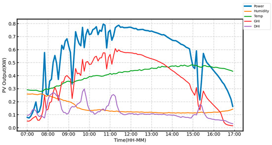
Figure 3.
The normalized meteorological data and photovoltaic output.
4.2. The Optimal Hyperparameters
In this study, Particle Swarm Optimization (PSO) is employed to optimize the parameters of the machine learning model used for PV power prediction. The ranges of these hyperparameters are described as follows. Hidden State Size : The number of units in the LSTM’s hidden state, which determines its capacity to capture complex temporal patterns in the PV power data. Head Size : The dimension of the query and key vectors in each attention head, affecting the granularity of the attention mechanism. Number of Heads : The number of separate attention heads, which allows the model to capture diverse dependencies in the data. Feed-Forward Dimension (FF Dim) : The size of the hidden layer in the feed-forward neural network, which influences the model’s ability to learn complex representations. Filters : The number of convolutional kernels in each layer, enabling the extraction of a richer set of temporal features. Kernel Size : The receptive field of the convolutional layer, controlling the temporal range of dependencies the model can capture. Dropout Rate : The fraction of neurons randomly deactivated during training to prevent overfitting. The number of layers for both the LSTM and TCN models was not included as part of the hyperparameter optimization. This choice was guided by the observation that increasing the number of layers often leads to higher computational costs and greater risk of overfitting without guaranteeing significant performance improvements, particularly for tasks with moderate data complexity like PV power prediction. A single-layer architecture was deemed sufficient to capture the temporal dependencies in the data while maintaining computational efficiency and reducing the model’s complexity. These hyperparameters are tuned to achieve optimal performance of the hybrid model for PV power prediction, ensuring effective modeling of both temporal and spatial dependencies in the data. The optimal hyperparameters of the models involved in this experiment can be seen in Table 1.

Table 1.
The optimal hyperparameters of the models.
4.3. Ablation and Comparison Experiments
4.3.1. Point-Forecasting Result
To analyze and evaluate the contribution of each component in the model, this paper compares the point prediction results of the sub-model with optimal hyperparameters and the Attention-Bi-LSTM model used in other studies [30]. The sub-models include the TCN, LSTM, Attention-TCN and TCN-LSTM. In the ablation experiments, to emphasize the superiority of the Attention-TCN-LSTM architecture, the number of layers in the sub-networks was fixed. This decision ensures a fair comparison by isolating the impact of the attention mechanism and the bidirectional design. By keeping the network depth constant, variations in performance can be more confidently attributed to the architectural enhancements introduced by the Attention-TCN-LSTM model, rather than differences in network complexity or capacity. Their respective point-forecasting results are shown in Figure 4.
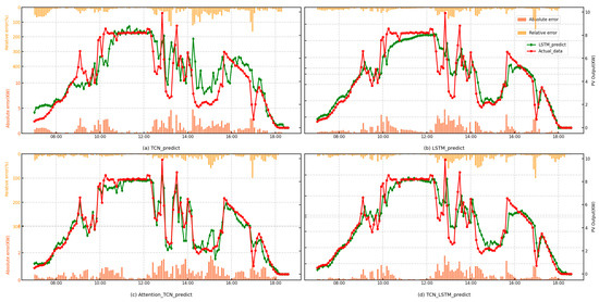
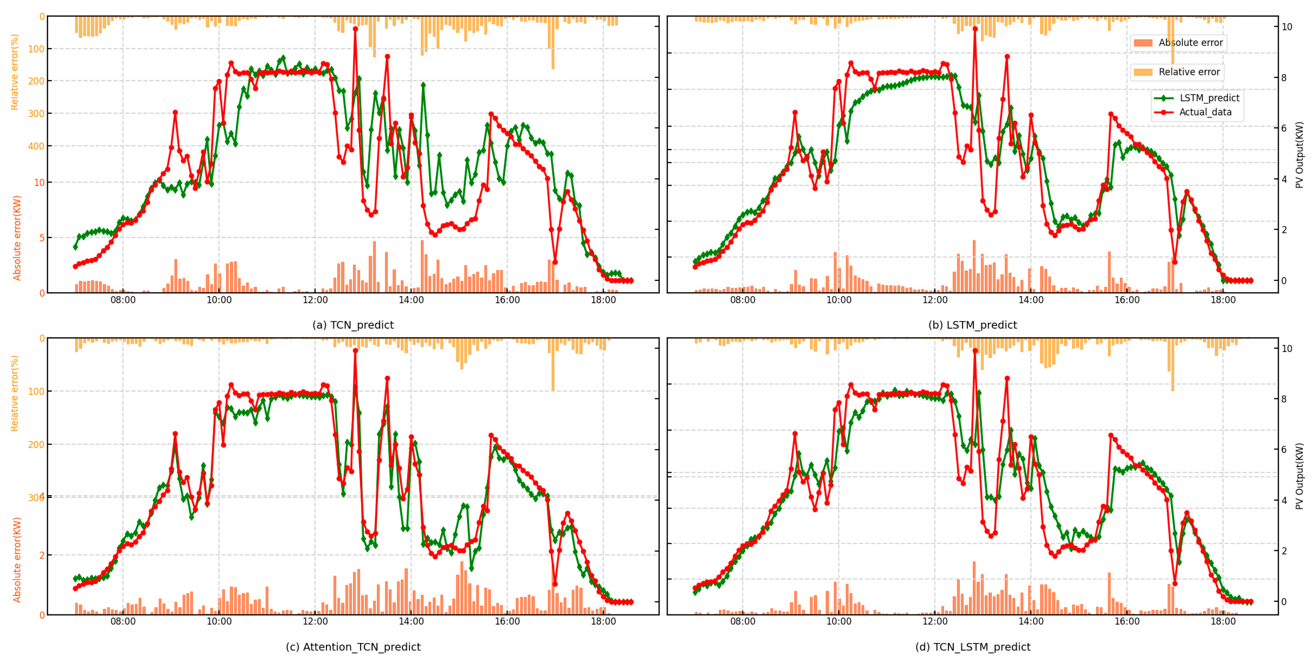
Figure 4.
Point-forecasting curves of the sub-models.
From the point prediction curves, it can be observed that the TCN and the LSTM models exhibit different characteristics. The TCN tends to capture rapid fluctuations, while the LSTM produces smoother predictions. The TCN, through convolution operations, is effective at capturing local features in time series data, making it highly sensitive to short-term fluctuations. This sensitivity to local changes likely explains the rapid fluctuations in its predictions. On the other hand, the LSTM, with its strong ability to remember long-term dependencies, may overly rely on past inputs, leading to smoother predictions, especially when the data exhibits stable long-term trends. While the LSTM is effective at capturing long-term patterns, it may struggle to respond to short-term fluctuations, resulting in smoother prediction outcomes. By incorporating the attention mechanism from the Transformer into the TCN, the model is able to more accurately follow the changing trends in the prediction curves. Similarly, combining the TCN with the LSTM can achieve the same effect, enhancing the model’s ability to capture both short-term fluctuations and long-term trends. The point-forecasting results of the proposed model and the comparison model are shown in Figure 5, respectively.
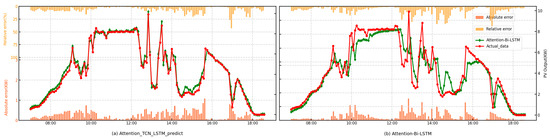
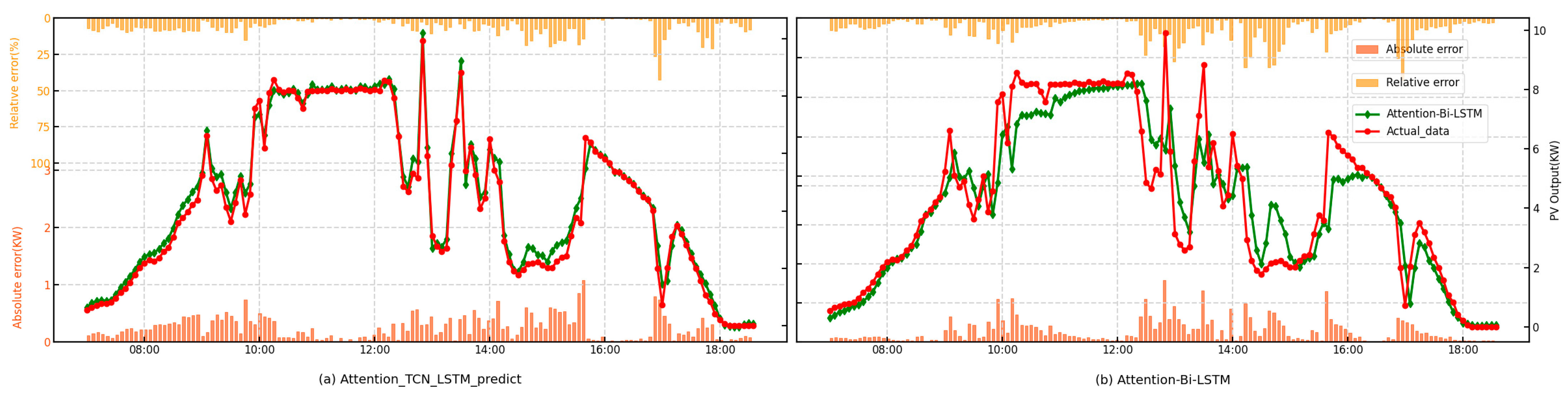
Figure 5.
Point-forecasting curves of the proposed model and the Attention-Bi-LSTM model.
It is evident from the prediction curves that the Attention-TCN-LSTM model, which combines the TCN and the LSTM, achieves the highest prediction accuracy. The LSTM captures long-term dependencies in photovoltaic output, making it effective for forecasting power generation. Attention-TCN, on the other hand, processes meteorological data, using the TCN to capture patterns and the attention mechanism to focus on key weather factors like temperature and radiation. Although Attention-Bi-LSTM shares similar characteristics, Attention-TCN-LSTM slightly outperforms it in terms of performance. Attention-Bi-LSTM excels at capturing bidirectional dependencies and leveraging attention for weighted feature extraction, making it suitable for tasks with long-term dependencies and complex sequences. However, Attention-TCN-LSTM combines the TCN’s powerful ability to capture local patterns with the attention mechanism’s adaptive focus on key features, making it more effective in handling data with rapid fluctuations and long sequences, leading to higher prediction accuracy.
As shown in Table 2, the Attention-TCN-LSTM model outperforms other models across all evaluation metrics. The RMSE and MAE are improved by 24% and 28%, respectively, compared to Attention-Bi-LSTM.
Table 2.
The point-forecasting results of the proposed model and the comparison model.
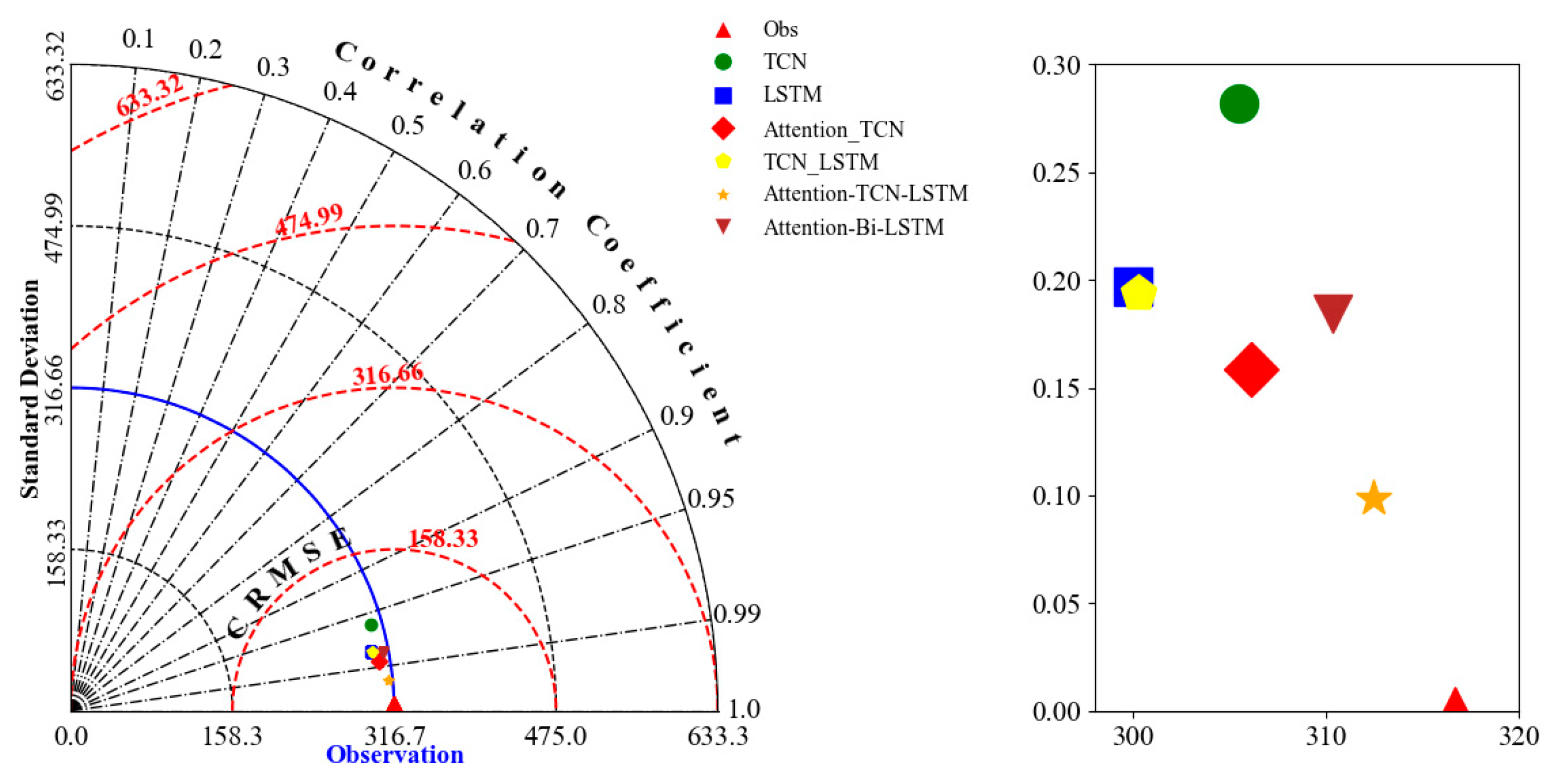
The results of all the models presented in this study are summarized in the Taylor diagram, as shown in Figure 6. The Taylor diagram is a graphical tool commonly used to evaluate the performance of predictive models by simultaneously displaying the correlation coefficient, standard deviation, and RMSE. It uses polar coordinates to represent the correlation coefficient along the angular axis and the standard deviation along the radial axis, while the distance between the model points and the reference point indicates the RMSE. A correlation coefficient closer to 1 suggests a stronger relationship between the model and observed data, a standard deviation closer to the reference indicates better representation of data variability, and a smaller RMSE reflects lower prediction error. The Taylor diagram’s strength lies in its ability to visually compare multiple models on a single plot, making it an effective tool for assessing model performance. The Taylor diagram further illustrates that the Attention model exhibits the smallest difference between its predictions and the observed data. As shown in the Figure 6, based on the evaluation criteria of the Taylor diagram, the proposed model’s prediction results are not only superior to the sub-model but also better than the comparison model.

Figure 6.
The Taylor Figure.
4.3.2. Interval-Forecasting Result
Interval prediction enhances operational decision-making by providing a range of possible outcomes for renewable energy generation. Wider prediction intervals offer higher confidence but may lead to overestimation of energy needs, requiring more storage capacity and backup power, which can result in inefficiencies and higher operational costs. On the other hand, narrower intervals provide more precise forecasts, reducing resource wastage but introducing the risk of underestimating energy needs, which could lead to grid instability or inadequate power supply. This trade-off between accuracy and reliability is crucial in energy storage management, grid stability, demand response, and risk mitigation. Narrower intervals may reduce costs and improve operational efficiency but increase the risk of missing critical fluctuations, while wider intervals offer more reliable coverage but at the expense of higher resource allocation and costs. Overall, interval predictions allow for more proactive, efficient, and reliable management of energy resources, with the width of the interval directly influencing decision-making strategies and resource optimization.
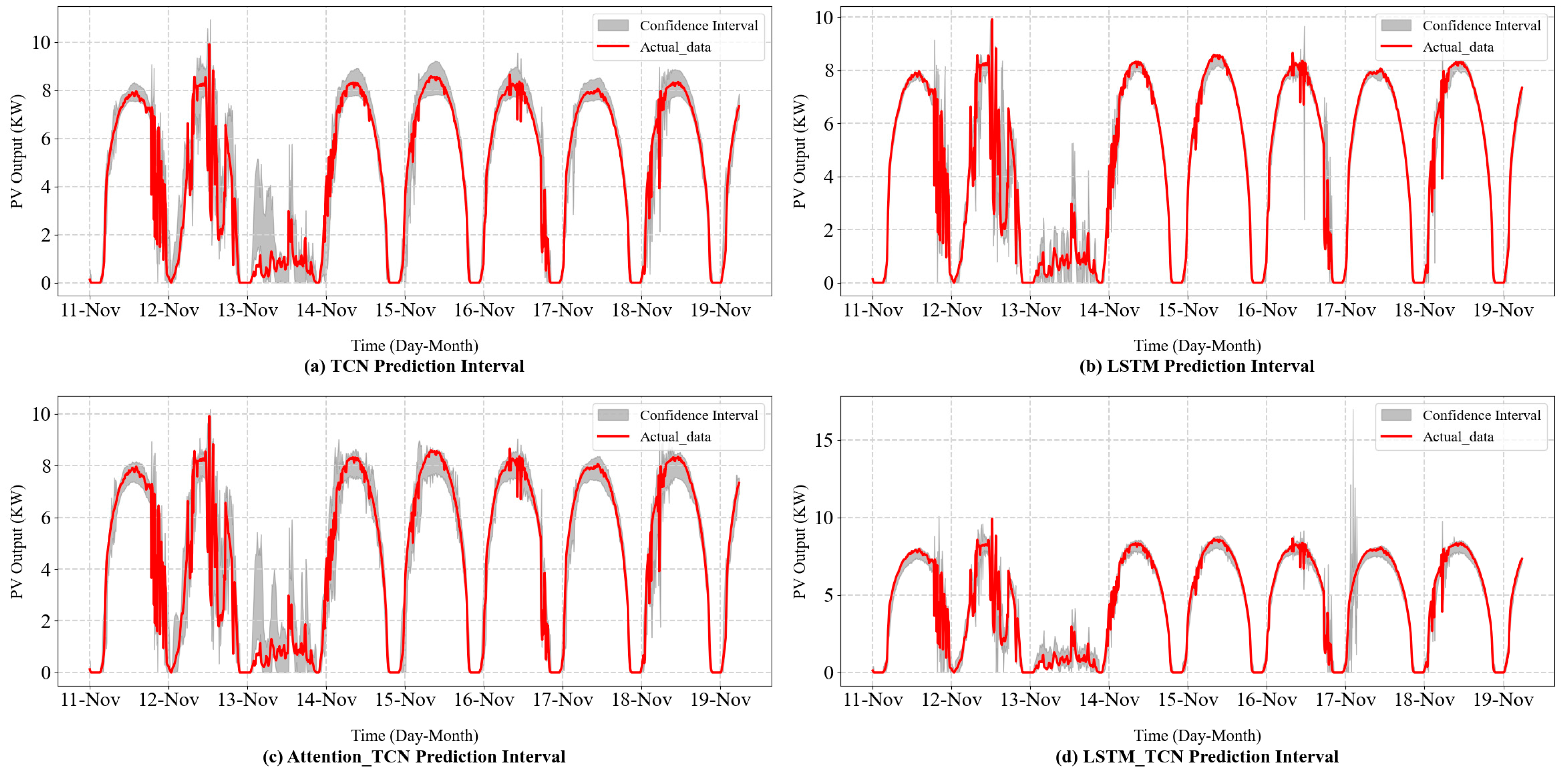
The bootstrap method serves as an effective approach to quantify the uncertainty in prediction results. Therefore, this study first performs point predictions and then constructs an interval prediction model using the bootstrap residual resampling method. By repeatedly resampling the dataset, the distribution range of the data samples is determined, enabling the construction of prediction intervals that address the limitation of deterministic prediction methods in representing the reliability of the results.
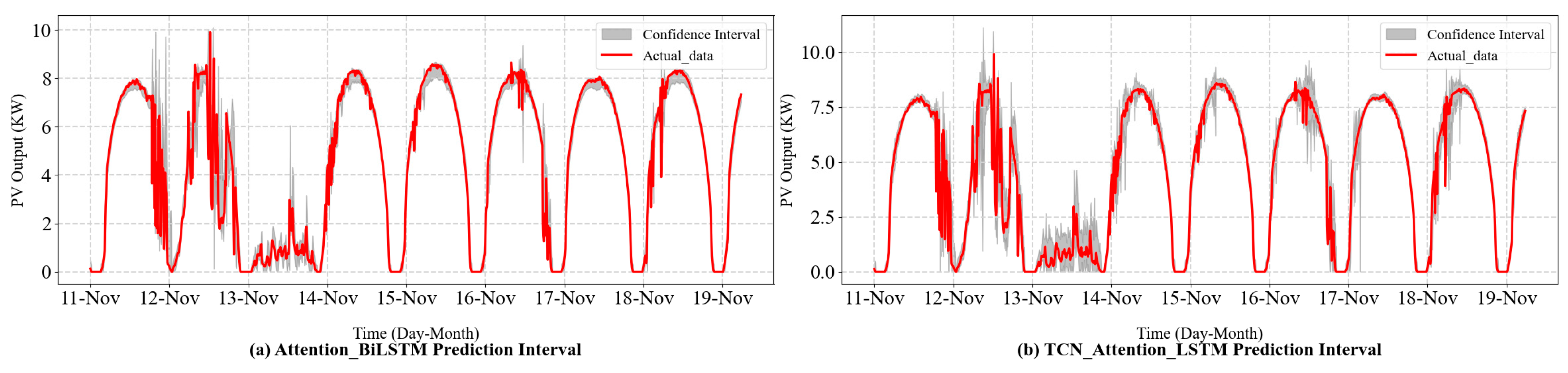
As shown in Figure 7 and Figure 8 and Table 3, all models except the LSTM model achieve high interval coverage rates, with PICP values exceeding the 85% confidence level. Compared to the Attention-Bi-LSTM model, the Attention-TCN-LSTM model demonstrates a higher PICP and a lower MPIW. The Attention-TCN-LSTM method balances interval width and coverage rate, achieving a comprehensive width-range index of 1.00, making it the best among the compared models. In contrast, when the Attention-Bi-LSTM model is applied for interval prediction, its PICP falls below 90%, indicating potential under-fitting. This could lead to reduced generalization ability and increased prediction errors on the test set. These results indicate that the proposed model not only achieves high interval coverage rates but also constructs more reasonable prediction intervals.

Figure 7.
Interval-forecasting curves of the sub-models.
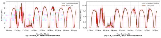
Figure 8.
Interval-forecasting curves of the proposed model and the Attention-Bi-LSTM model.
Table 3.
The Interval-forecasting results of the proposed model and the comparison model.
5. Conclusions
The increase in PV penetration exacerbates the complexity of the power system supply–demand balance due to its randomness, volatility, and intermittency, potentially causing issues such as overvoltage in distribution networks. Photovoltaic forecasting plays a crucial role in ensuring the stability and efficiency of power systems, making it an essential area of research and development.
This study introduces a hybrid Attention-TCN-LSTM model to forecast the PV power. The proposed approach leverages the strengths of both the TCN and the LSTM and the self-attention mechanism of Transformer module to enhance forecasting accuracy. The hybrid model can capture the inherent variability in photovoltaic (PV) output and meteorological conditions. In order to avoid the influence of model hyperparameters on the prediction results, the PSO algorithm is used to find the optimal hyperparameters. To assess the uncertainty of PV power predictions, this study employs the bootstrap method by reconstructing the input data using prediction biases. The proposed algorithm achieves a root mean square error (RMSE) value of 0.363, a mean absolute error (MAE) value of 0.161, and an R-squared (R2) value of 0.98. This highlights its superiority in balancing accuracy and reliability in point prediction. Additionally, the proposed model constructs narrower prediction intervals while maintaining high interval coverage rates with a Comprehensive Width Coverage (CWC) of 1.00. In interval prediction, the proposed model demonstrates excellent performance, ensuring both precision and reliability in uncertainty quantification. However, both the more accurate single-point prediction model and the more reliable interval prediction model have their limitations to uncertainty analysis. A key focus for future research is exploring how to integrate interval prediction with intelligent systems to enable autonomous control and manage uncertain risks during the dynamic changes in photovoltaic output sequences.
Author Contributions
Conceptualization, Y.G., X.W. and Y.S.; methodology, H.Q.; software, H.Q.; validation, H.Q., L.W. and Z.L.; writing—original draft preparation, H.Q.; writing—review and editing, Z.L.; visualization, Z.L.; supervision, Y.S.; project administration, Y.G.; funding acquisition, L.W. All authors have read and agreed to the published version of the manuscript.
Funding
This research was sponsored by the State Grid Corporation Headquarters Science and Technology Project (4000-202424078A-1-1-ZN).
Data Availability Statement
PV plant operators require data to be kept confidential.
Conflicts of Interest
The authors declare no conflicts of interest. The funders had no role in the design of the study; in the collection, analyses, or interpretation of data; in the writing of the manuscript; or in the decision to publish the results.
References
- Shakya, A.; Michael, S.; Saunders, C.; Armstrong, D.; Pandey, P.; Chalise, S.; Tonkoski, R. Solar Irradiance Forecasting in Remote Microgrids Using Markov Switching Model. IEEE Trans. Sustain. Energy 2017, 8, 895–905. [Google Scholar] [CrossRef]
- van der Meer, D.W.; Widén, J.; Munkhammar, J. Review on Probabilistic Forecasting of Photovoltaic Power Production and Electricity Consumption. Renew. Sustain. Energy Rev. 2018, 81, 1484–1512. [Google Scholar] [CrossRef]
- Wang, L.; Bai, F.; Yan, R.; Saha, T.K. Real-Time Coordinated Voltage Control of PV Inverters and Energy Storage for Weak Networks with High PV Penetration. IEEE Trans. Power Syst. 2018, 33, 3383–3395. [Google Scholar] [CrossRef]
- Wu, Y.-K.; Phan, Q.-T.; Zhong, Y.-J. Overview of Day-Ahead Solar Power Forecasts Based on Weather Classifications and a Case Study in Taiwan. IEEE Trans. Ind. Appl. 2024, 60, 1409–1423. [Google Scholar] [CrossRef]
- Wang, L.; Wang, T.; Huang, G.; Wang, K.; Yan, R.; Zhang, Y. Softly Collaborated Voltage Control in PV Rich Distribution Systems With Heterogeneous Devices. IEEE Trans. Power Syst. 2024, 39, 5991–6003. [Google Scholar] [CrossRef]
- Liu, Z.-F.; Luo, S.-F.; Tseng, M.-L.; Liu, H.-M.; Li, L.; Mashud, A.H.M. Short-Term Photovoltaic Power Prediction on Modal Reconstruction: A Novel Hybrid Model Approach. Sustain. Energy Technol. Assess. 2021, 45, 101048. [Google Scholar] [CrossRef]
- Wang, L.; Xie, L.; Yang, Y.; Zhang, Y.; Wang, K.; Cheng, S. Distributed Online Voltage Control With Fast PV Power Fluctuations and Imperfect Communication. IEEE Trans. Smart Grid 2023, 14, 3681–3695. [Google Scholar] [CrossRef]
- Antonanzas, J.; Osorio, N.; Escobar, R.; Urraca, R.; Martinez-de-Pison, F.J.; Antonanzas-Torres, F. Review of Photovoltaic Power Forecasting. Sol. Energy 2016, 136, 78–111. [Google Scholar] [CrossRef]
- Wolff, B.; Kühnert, J.; Lorenz, E.; Kramer, O.; Heinemann, D. Comparing Support Vector Regression for PV Power Forecasting to a Physical Modeling Approach Using Measurement, Numerical Weather Prediction, and Cloud Motion Data. Sol. Energy 2016, 135, 197–208. [Google Scholar] [CrossRef]
- Nelega, R.; Greu, D.I.; Jecan, E.; Rednic, V.; Zamfirescu, C.; Puschita, E.; Turcu, R.V.F. Prediction of Power Generation of a Photovoltaic Power Plant Based on Neural Networks. IEEE Access 2023, 11, 20713–20724. Available online: https://ieeexplore.ieee.org/document/10054046 (accessed on 18 November 2024). [CrossRef]
- Das, U.K.; Tey, K.S.; Seyedmahmoudian, M.; Idna Idris, M.Y.; Mekhilef, S.; Horan, B.; Stojcevski, A. SVR-Based Model to Forecast PV Power Generation under Different Weather Conditions. Energies 2017, 10, 876. [Google Scholar] [CrossRef]
- Moreira, M.O.; Balestrassi, P.P.; Paiva, A.P.; Ribeiro, P.F.; Bonatto, B.D. Design of Experiments Using Artificial Neural Network Ensemble for Photovoltaic Generation Forecasting. Renew. Sustain. Energy Rev. 2021, 135, 110450. [Google Scholar] [CrossRef]
- Zheng, L.; Su, R.; Sun, X.; Guo, S. Historical PV-Output Characteristic Extraction Based Weather-Type Classification Strategy and Its Forecasting Method for the Day-Ahead Prediction of PV Output. Energy 2023, 271, 127009. [Google Scholar] [CrossRef]
- Agga, A.; Abbou, A.; Labbadi, M.; El Houm, Y. Short-Term Self Consumption PV Plant Power Production Forecasts Based on Hybrid CNN-LSTM, ConvLSTM Models. Renew. Energy 2021, 177, 101–112. [Google Scholar] [CrossRef]
- Wang, X.; Ma, W. A Hybrid Deep Learning Model with an Optimal Strategy Based on Improved VMD and Transformer for Short-Term Photovoltaic Power Forecasting. Energy 2024, 295, 131071. [Google Scholar] [CrossRef]
- Lai, W.; Zhen, Z.; Wang, F.; Fu, W.; Wang, J.; Zhang, X.; Ren, H. Sub-Region Division Based Short-Term Regional Distributed PV Power Forecasting Method Considering Spatio-Temporal Correlations. Energy 2024, 288, 129716. [Google Scholar] [CrossRef]
- Konstantinou, M.; Peratikou, S.; Charalambides, A.G. Solar Photovoltaic Forecasting of Power Output Using LSTM Networks. Atmosphere 2021, 12, 124. [Google Scholar] [CrossRef]
- Ren, X.; Liu, Y.; Zhang, F.; Li, L. A Deep Learning Quantile Regression Photovoltaic Power-Forecasting Method under a Priori Knowledge Injection. Energies 2024, 17, 4026. [Google Scholar] [CrossRef]
- Benitez, I.B.; Ibañez, J.A.; Lumabad, C.I.D.; Cañete, J.M.; Principe, J.A. Day-Ahead Hourly Solar Photovoltaic Output Forecasting Using SARIMAX, Long Short-Term Memory, and Extreme Gradient Boosting: Case of the Philippines. Energies 2023, 16, 7823. [Google Scholar] [CrossRef]
- Pei, Y.; Zhao, J.; Yao, Y.; Ding, F. Multi-Task Reinforcement Learning for Distribution System Voltage Control With Topology Changes. IEEE Trans. Smart Grid 2023, 14, 2481–2484. [Google Scholar] [CrossRef]
- Short-Term Electric Load Forecasting Based on EEMD-GRU-MLR-All Databases. Available online: https://webofscience.clarivate.cn/wos/alldb/full-record/CSCD:6670349 (accessed on 18 November 2024).
- Photovoltaic Power Forecasting Based on GA Improved Bi-LSTM in Microgrid without Meteorological Information. Energy 2021, 231, 120908. [CrossRef]
- Eseye, A.T.; Zhang, J.; Zheng, D. Short-Term Photovoltaic Solar Power Forecasting Using a Hybrid Wavelet-PSO-SVM Model Based on SCADA and Meteorological Information. Renew. Energy 2018, 118, 357–367. [Google Scholar] [CrossRef]
- Das, U.K.; Tey, K.S.; Seyedmahmoudian, M.; Mekhilef, S.; Idris, M.Y.I.; Van Deventer, W.; Horan, B.; Stojcevski, A. Forecasting of Photovoltaic Power Generation and Model Optimization: A Review. Renew. Sustain. Energy Rev. 2018, 81, 912–928. [Google Scholar] [CrossRef]
- Xu, W.; Li, D.; Dai, W.; Wu, Q. Informer Short-Term PV Power Prediction Based on Sparrow Search Algorithm Optimised Variational Mode Decomposition. Energies 2024, 17, 2984. [Google Scholar] [CrossRef]
- Tao, K.; Zhao, J.; Tao, Y.; Qi, Q.; Tian, Y. Operational Day-Ahead Photovoltaic Power Forecasting Based on Transformer Variant. Appl. Energy 2024, 373, 123825. [Google Scholar] [CrossRef]
- Li, Y.; Song, L.; Zhang, S.; Kraus, L.; Adcox, T.; Willardson, R.; Komandur, A.; Lu, N. A TCN-Based Hybrid Forecasting Framework for Hours-Ahead Utility-Scale PV Forecasting. IEEE Trans. Smart Grid 2023, 14, 4073–4085. [Google Scholar] [CrossRef]
- La Rocca, M.; Giordano, F.; Perna, C. Clustering Nonlinear Time Series with Neural Network Bootstrap Forecast Distributions. Int. J. Approx. Reason. 2021, 137, 1–15. [Google Scholar] [CrossRef]
- Yamamoto, H.; Kondoh, J.; Kodaira, D. Assessing the Impact of Features on Probabilistic Modeling of Photovoltaic Power Generation. Energies 2022, 15, 5337. [Google Scholar] [CrossRef]
- He, B.; Ma, R.; Zhang, W.; Zhu, J.; Zhang, X. An Improved Generating Energy Prediction Method Based on Bi-LSTM and Attention Mechanism. Electronics 2022, 11, 1885. [Google Scholar] [CrossRef]

Disclaimer/Publisher’s Note: The statements, opinions and data contained in all publications are solely those of the individual author(s) and contributor(s) and not of MDPI and/or the editor(s). MDPI and/or the editor(s) disclaim responsibility for any injury to people or property resulting from any ideas, methods, instructions or products referred to in the content. |
© 2025 by the authors. Licensee MDPI, Basel, Switzerland. This article is an open access article distributed under the terms and conditions of the Creative Commons Attribution (CC BY) license (https://creativecommons.org/licenses/by/4.0/).